Violations of locality and free choice are equivalent resources in Bell experiments

Abstract

Bell inequalities rest on three fundamental assumptions: realism, locality, and free choice, which lead to nontrivial constraints on correlations in very simple experiments. If we retain realism, then violation of the inequalities implies that at least one of the remaining two assumptions must fail, which can have profound consequences for the causal explanation of the experiment. We investigate the extent to which a given assumption needs to be relaxed for the other to hold at all costs, based on the observation that a violation need not occur on every experimental trial, even when describing correlations violating Bell inequalities. How often this needs to be the case determines the degree of, respectively, locality or free choice in the observed experimental behavior. Despite their disparate character, we show that both assumptions are equally costly. Namely, the resources required to explain the experimental statistics (measured by the frequency of causal interventions of either sort) are exactly the same. Furthermore, we compute such defined measures of locality and free choice for any nonsignaling statistics in a Bell experiment with binary settings, showing that it is directly related to the amount of violation of the so-called Clauser-Horne-Shimony-Holt inequalities. This result is theory independent as it refers directly to the experimental statistics. Additionally, we show how the local fraction results for quantum-mechanical frameworks with infinite number of settings translate into analogous statements for the measure of free choice we introduce. Thus, concerning statistics, causal explanations resorting to either locality or free choice violations are fully interchangeable.

10(7.8,0.5) For published version see PNAS 118 (17) e2020569118 (2021)

"I would rather discover one true cause
than gain the kingdom of Persia."

– Democritus (c. 460-370 BC)

The study of experimental correlations provides a window into the underlying causal mechanisms, even when their exact nature remains obscured. In his seminal works (1, 2, 3, 4, 5), John Bell showed that seemingly innocuous assumptions about the structure of causal relationships leave a mark on the observed statistics. The first assumption, called realism (or counterfactual definiteness), presents the worldview in which physical objects and their properties exist, whether they are observed or not. Note that realism allows a standard notion of causality (6, 7), which in turn provides us with the language to express the remaining two assumptions. The locality assumption is a statement that physical (or causal) influences propagate in accord with the spatio-temporal structure of events (i.e., neither backward in time nor instantaneous causation). The free choice assumption asserts that the choice of measurement settings can be made independently from anything in the (causal) past. These three assumptions are enough to derive testable constraints on correlations called Bell inequalities.

Surprisingly, nature violates Bell inequalities (8, 9, 10, 11, 12, 13, 14, 15) which means that if the standard causal (or realist) picture is to be maintained at least one of the remaining two assumptions, that is locality or free choice, has to fail. It turns out that rejecting just one of those two assumptions is always enough to explain the observed correlations, while maintaining consistency with the causal structure imposed by the other. Either option poses a challenge to deep-rooted intuitions about reality, with a full range of viable positions open to serious philosophical dispute (16, 17, 18). Notably, quantum theory in its operational formulation does not provide any clue regarding the causal structure at work, leaving such questions to the domain of interpretation. It is therefore interesting to ask about the extent to which a given assumption needs to be relaxed, if we insist on upholding the other one (while always maintaining realism). In this paper, we seek to compare the cost of locality and free choice on an equal footing, without any preconceived conceptual biases. As a basis for comparison we choose to measure the weight of a given assumption in terms of the following question:

How often a given assumption, i.e. locality or free choice, can be retained, while safeguarding the other assumption, in order to fully reproduce some given experimental statistics within a standard causal (or realist) approach?

This question presumes that a Bell experiment is performed trial-by-trial and the observed statistics can be explained in the standard causal model (or hidden variable) framework (1, 2, 3, 4, 5, 6, 7, 19, 20, 21), which subsumes realism. It means that the remaining two assumptions of locality and free choice translate into conditional independence between certain variables in the model, whose causal structure is determined by their spatio-temporal relations (6, 22) (for some alternative approach endorsing indefinite causal structures see e.g. (23, 24), or (25) for discussion of retrocausality). Modelling of the experiment implies that in each run of the experiment all variables (including unobserved or hidden ones) always take definite values and the statistics accumulates over many trials. This leaves open the possibility that the violation of the assumptions do not have to occur on each run of the experiment to explain the given statistics. We can thus put flesh on the bones of the above question and seek the maximal proportion of trials in which a given assumption can be retained, while safeguarding the other assumption, so as to fully reproduce some given statistics. In the following, we shall denote so defined measure of locality (safeguarding freedom of choice) as $\mu_{\scriptscriptstyle L}$ and measure of free choice (safeguarding locality) as $\mu_{\scriptscriptstyle F}$. Also, without stating this in every instance, we note that in all subsequent discussion realism is assumed.

There has been some previous research on this theme. A measure of locality analogous to $\mu_{\scriptscriptstyle L}$ was first proposed by Elitzur, Popescu and Rohrlich (27) to quantify non-locality in a singlet state. Note, it seems that the original idea of a bound for such a locality measure was expressed earlier, in (28), but a bound was not worked out. In any case, Elitzur, Popescu, and Rohrlich’s measure was dubbed local fraction (or content) and shown (with improvements in (29, 30, 31)) to vanish in the limit of an infinite number of measurement settings. A substantial step was made in (32) where the local fraction is explicitly calculated for any pure two-qubit state for an arbitrary choice of settings. We note that those results concern measure $\mu_{\scriptscriptstyle L}$ only for the specific case of quantum-mechanical predictions. In this paper we go beyond this framework and consider the case of general experimental statistics (see (33) for extension to the idea of contextuality). To avoid confusion, the term local fraction for measure $\mu_{\scriptscriptstyle L}$ will be only used in relation to the quantum case. Furthermore, we propose a similar treatment of the free choice assumption quantified by measure $\mu_{\scriptscriptstyle F}$. Natural as it may seem, this approach has not been pursued in the literature, with some other measures proposed to this effect (34, 35, 36, 35, 37, 38, 39, 40, 41, 42) (all retaining locality as a principle, but departing from the original notion of free choice introduced by Bell (6, 22)).

We aim to comprehensively consider the extent to which a given assumption, i.e. locality or free choice, can be preserved through partial violation of the other assumption. To accomplish this, we provide similar definitions and discuss on an equal footing both measures of locality $\mu_{\scriptscriptstyle L}$ and free choice $\mu_{\scriptscriptstyle F}$. Then, we derive the following results. First, we prove a general structural theorem about causal models explaining any given experimental statistics in a Bell experiment (for any number of settings) showing that such defined measures are necessarily equal, $\mu_{\scriptscriptstyle L}=\mu_{\scriptscriptstyle F}$. This result consolidates those two disparate concepts demonstrating their deep interchangeability. Second, we explicitly compute both measures for any non-signalling statistics in a two-setting and two-outcome Bell scenario. This enables a direct interpretation to the amount of violation of the Clauser-Horne-Shimony-Holt (CHSH) inequalities (43). Third, we consider the special case of the quantum statistics with infinite number of settings, utilising existing results for the local fraction $\mu_{\scriptscriptstyle L}$, which thus translate on the newly developed concept of the measure of free choice $\mu_{\scriptscriptstyle F}$. Fig. 1 summarises the results in the paper.

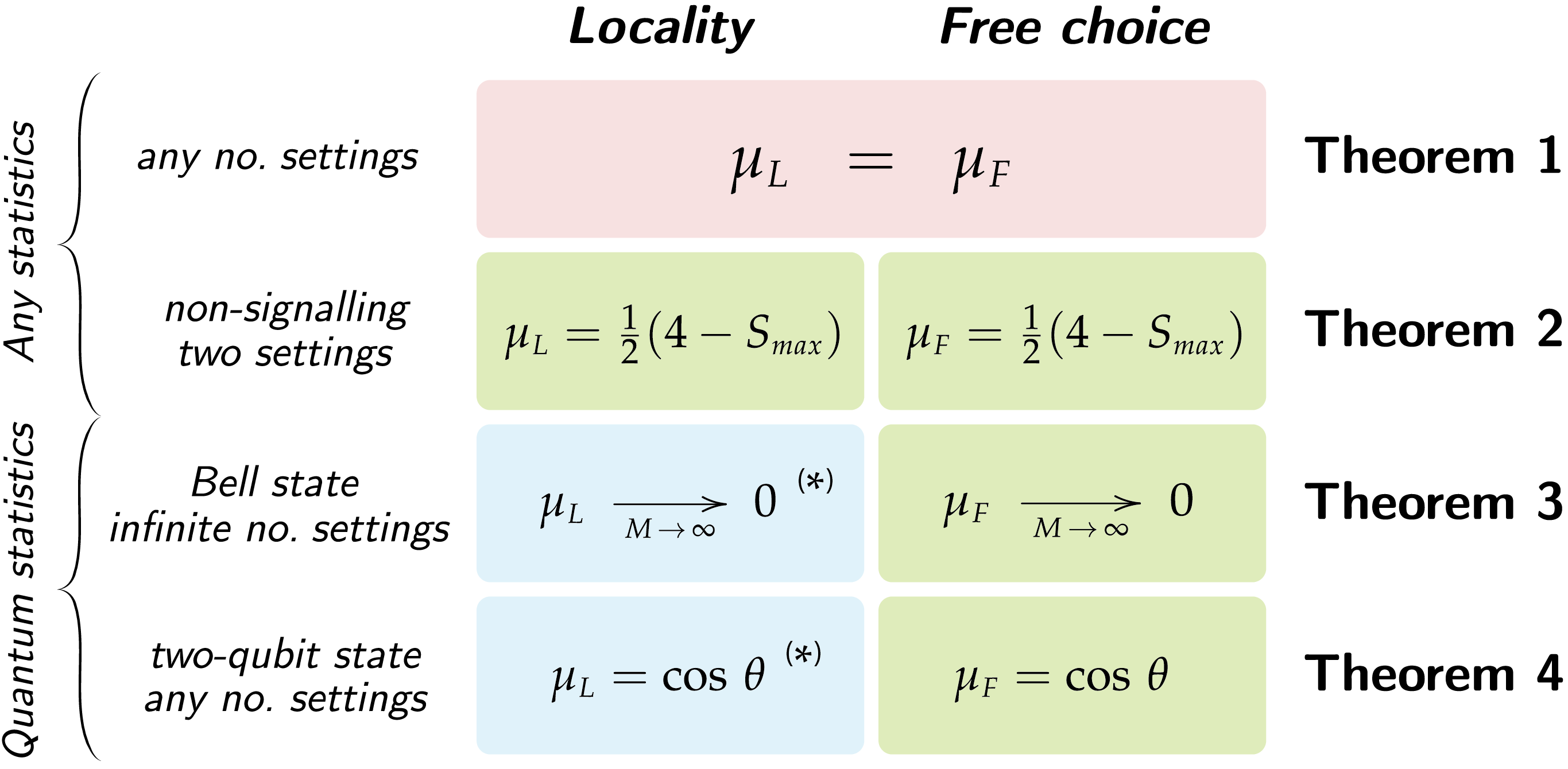
Figure 1: Summary of the results. The main Theorem 1 is the backbone of the paper, consolidating both measures of locality $\mu_{\scriptscriptstyle L}$ and free choice $\mu_{\scriptscriptstyle F}$. Theorem 2 is a theory-independent result about both measures $\mu_{\scriptscriptstyle L}$ and $\mu_{\scriptscriptstyle F}$. It offers a concrete interpretation for the amount of violation of the CHSH inequalities. Theorems 3 and 4 are specific to the quantum-mechanical statistics stated here for measure $\mu_{\scriptscriptstyle F}$. They are translations of some remarkable local fraction results $\mu_{\scriptscriptstyle L}$ in the literature (marked with an ^(∗), cf. (29, 30, 31, 32)).

Results

Bell experiment and Fine’s theorem

Let us consider the usual Bell-type scenario with two parties, called Alice and Bob, playing the roles of agents conducting experiments on two separated systems (whose nature is irrelevant for the argument). We assume that on each side there are two possible outcomes labelled respectively $a,b=\pm 1$ and $M$ possible measurement settings labelled respectively $x,y\in\mathfrak{M}$ where $\mathfrak{M}\equiv\{1,2\,,\dots,M\}$. A Bell experiment consists of a series of trials in which Alice and Bob each choose a setting and make a measurement registering the outcome. After many repetitions, they compare their results described by the set of $M\times M$ distributions $\{P_{\scriptscriptstyle ab|xy}\}_{\scriptscriptstyle xy}$ , where $P_{\scriptscriptstyle ab|xy}$ denotes the probability of obtaining outcomes $a,b$, given measurements $x,y$ were made on Alice and Bob’s side respectively. For conciseness, following the terminology in (5), we will call $\{P_{\scriptscriptstyle ab|xy}\}_{\scriptscriptstyle xy}$ a "behaviour". Note that without assuming anything about the causal structure underlying the experiment any behaviour is admissible (as long as the distributions are normalised, i.e. $\sum_{\scriptscriptstyle a,b}P_{\scriptscriptstyle ab|xy}=1$ for each $x,y\in\mathfrak{M}$). In particular, quantum theory gives a prescription for calculating the experimental statistics $P_{\scriptscriptstyle ab|xy}$ for each choice of settings $x,y\in\mathfrak{M}$ based on the formalism of Hilbert spaces.

It is instructive to recall the special case of two measurement settings on each side $x,y\in\mathfrak{M}=\{0,1\}$ for which Bell derived his seminal result. Briefly, this can be expressed by saying that any local hidden variable model with free choice has to satisfy the following four CHSH inequalities (43)

$$|S_{\scriptscriptstyle i}|\ \leqslant\ 2 \qquad\text{for\ \ $i=1,...\,,4$}\,,$$ (1)

where

$$S_{\scriptscriptstyle 1} \!\!=\!\! \ \ \ \langle ab\rangle_{\scriptscriptstyle 00}+\langle ab\rangle_{\scriptscriptstyle 01}+\langle ab\rangle_{\scriptscriptstyle 10}-\langle ab\rangle_{\scriptscriptstyle 11}\,,$$ (2)

$$S_{\scriptscriptstyle 2} \!\!=\!\! \ \ \ \langle ab\rangle_{\scriptscriptstyle 00}+\langle ab\rangle_{\scriptscriptstyle 01}-\langle ab\rangle_{\scriptscriptstyle 10}+\langle ab\rangle_{\scriptscriptstyle 11}\,,$$ (3)

$$S_{\scriptscriptstyle 3} \!\!=\!\! \ \ \ \langle ab\rangle_{\scriptscriptstyle 00}-\langle ab\rangle_{\scriptscriptstyle 01}+\langle ab\rangle_{\scriptscriptstyle 10}+\langle ab\rangle_{\scriptscriptstyle 11}\,,$$ (4)

$$S_{\scriptscriptstyle 4} \!\!=\!\! -\langle ab\rangle_{\scriptscriptstyle 00}+\langle ab\rangle_{\scriptscriptstyle 01}+\langle ab\rangle_{\scriptscriptstyle 10}+\langle ab\rangle_{\scriptscriptstyle 11}\,,$$ (5)

with $\langle ab\rangle_{\scriptscriptstyle xy}=\sum_{\scriptscriptstyle a,b}\,ab\,P_{\scriptscriptstyle ab|xy}$ being correlation coefficients for a given choice of settings $x,y$. Interestingly, by virtue of Fine’s theorem (44, 45), this is also a sufficient condition for a non-signalling behaviour $\{P_{\scriptscriptstyle ab|xy}\}_{\scriptscriptstyle xy}$ to be explained by a local hidden variable model with freedom of choice (for non-signalling see Eqs. (20) and (21)).

It is crucial to observe that, although locality and freedom of choice are two disparate concepts with different ramifications for our understanding of the experiment, they are in a certain sense interchangeable. If locality is dropped with Alice and Bob freely choosing their settings, then the boxes, by influencing one another, can produce any behaviour $\{P_{\scriptscriptstyle ab|xy}\}_{\scriptscriptstyle xy}$. Similarly, a violation of the free choice assumption can be used to reproduce any behaviour $\{P_{\scriptscriptstyle ab|xy}\}_{\scriptscriptstyle xy}$, without giving up locality. It is straightforward to see how this might work if one of the two assumptions fails on every experimental trial.

However, such a complete renouncement of assumptions so central to our view of nature may seem excessive, especially when the CHSH inequalities are violated only by a little amount (less than the maximal algebraic bound of $|S_{\scriptscriptstyle i}|\leqslant 4$), leaving room for a possible explanation of the experimental statistics by rejecting one of the assumptions sometimes only. Here we assess the cost of such a partial violation by asking how often a given assumption can be retained in order to account for a behaviour $\{P_{\scriptscriptstyle ab|xy}\}_{\scriptscriptstyle xy}$ . We will investigate both cases in parallel: ($\scriptstyle\spadesuit$ ‣ Bell experiment and Fine’s theorem) full freedom of choice with occasional non-locality (communication), and ($\scriptstyle\clubsuit$ ‣ Bell experiment and Fine’s theorem) the possibility of retaining full locality at a price of compromising freedom of choice (by controlling or rigging measurement settings) on some of the trials. We shall use the least frequency of violation, required to model some statistics with a hypothetical simulation, as a natural figure of merit, guided by the principle that the less the violation the better. Notably, such simulations should not restrict possible distributions of measurement settings $P_{\scriptscriptstyle xy}$. In other words, we define a measure of locality $\mu_{\scriptscriptstyle L}$ as

the maximal fraction of trials in which Alice and Bob do not need to communicate trying to simulate a given behaviour $$\{P_{\scriptscriptstyle ab|xy}\}_{\scriptscriptstyle xy} \scriptstyle\spadesuit$$ , optimised over all conceivable strategies with freely chosen settings.     ()

Similarly, we define a measure of free choice $\mu_{\scriptscriptstyle F}$ as

the maximal fraction of trials in which Alice and Bob can grant free choice of settings in trying to simulate a given behaviour $$\{P_{\scriptscriptstyle ab|xy}\}_{\scriptscriptstyle xy} \scriptstyle\clubsuit$$ , optimised over all conceivable local strategies.     ()

In the quantum-mechanical context the measure $\mu_{\scriptscriptstyle L}$ is called a local fraction (27, 28, 29, 30, 31, 32). By analogy, when considering the quantum-mechanical statistics the measure $\mu_{\scriptscriptstyle F}$ might be called a free fraction. This provides an equal basis for comparing the two assumptions within the standard causal (or realist) approach, which we formalise in the following section.

Causal models, locality and free choice

The appropriate framework for the discussion of locality and free choice is provided by hidden variable models (1, 2, 3, 4, 5). First, a hidden variables model allows a formal statement of the realism assumption, understood to mean that properties of a physical system exist irrespective of an act of measurement (counterfactual definiteness). Second, hidden variable models provide the causal language in which the locality and free choice assumptions are expressed (6, 7). The locality assumption conveys the requirement that the propagation of physical (or causal) influences have to follow the spatio-temporal structure of events (i.e., preserve the arrow of time and respect that actions at a distance require time). The free choice assumption concerns the choice of measurement settings which are deemed cusally unaffected by anything in the past (and thus it is sometimes called measurement independence). Both assumptions take the form of conditional independencies between certain variables in a hidden variables model.

To make this idea more concrete, let us consider a given set of probability distributions (behaviour) $\{P_{\scriptscriptstyle ab|xy}\}_{\scriptscriptstyle xy}$ which describes the statistics in a Bell experiment. Without loss of generality, by conditioning on $\lambda$ in some a priori unknown hidden variable space $\Lambda$, one can always write (4, 5, 7)

$$P_{\scriptscriptstyle ab|xy}\ =\ \sum_{\scriptscriptstyle\lambda\in\Lambda}P_{\scriptscriptstyle ab|xy\lambda}\cdot P_{\scriptscriptstyle\lambda|xy}\,,$$ (6)

where $P_{\scriptscriptstyle\lambda|xy}$ and $P_{\scriptscriptstyle ab|xy\lambda}$ are valid (i.e. normalised) conditional probability distributions. The role of the hidden variable (cause in the past) $\lambda\in\Lambda$, distributed according to some $P_{\scriptscriptstyle\lambda}$, is to provide an explanation of the observed experimental statistics. This means that at each run of the experiment the outcomes are described by the distribution $P_{\scriptscriptstyle ab|xy\lambda}$ with $\lambda\in\Lambda$ fixed in a given trial, so that the accumulated experimental statistics $P_{\scriptscriptstyle ab|xy}$ obtains by sampling from some distribution $P_{\scriptscriptstyle\lambda|xy}$ over the whole hidden variable space $\Lambda$. It is customary to say that

the choice of space $$\Lambda P_{\scriptscriptstyle\lambda} P_{\scriptscriptstyle ab|xy\lambda} P_{\scriptscriptstyle\lambda|xy} \{P_{\scriptscriptstyle ab|xy}\}_{\scriptscriptstyle xy} \star$$ and probability distribution along with conditional distributions and satisfying Eq. (6) specify a hidden variable (HV) model of a given behaviour  .     ()

Note that such a model implicitly describes the distribution of settings chosen by Alice and Bob through the standard formula

$$P_{\scriptscriptstyle xy}\ =\ \sum_{\scriptscriptstyle\lambda\in\Lambda}P_{\scriptscriptstyle xy|\lambda}\cdot P_{\scriptscriptstyle\lambda}\,.$$ (7)

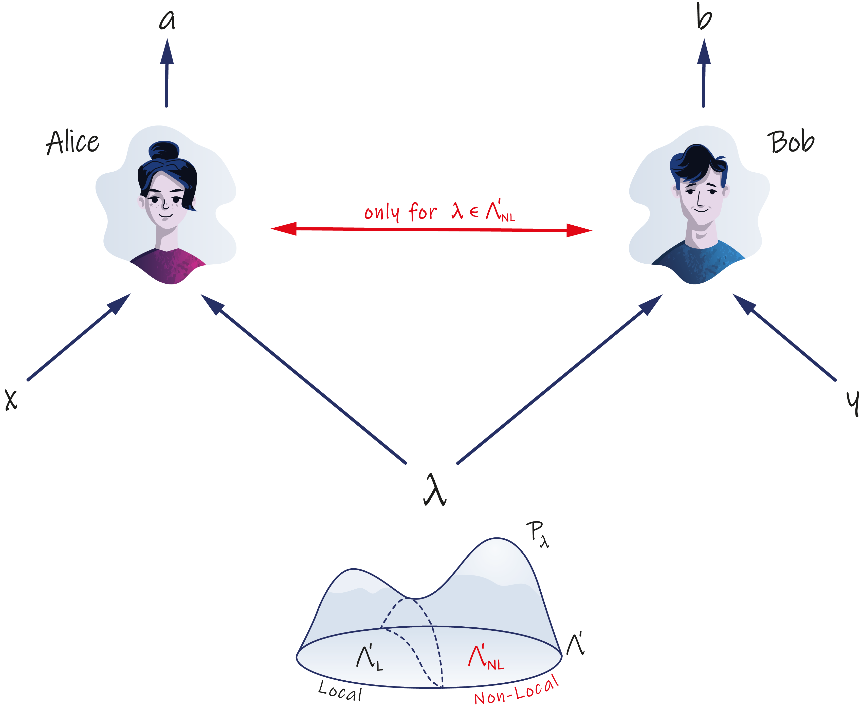
Figure 2: Causal model with some non-locality (communication). In a Bell scenario, with free choice of settings, correlations between Alice and Bob’s outcomes have two possible explanations: common cause in the past or causal influence between the parties. In any causal model the space of hidden variables (representing common causes) splits into two disjoint parts $\Lambda^{\prime}=\Lambda^{\prime}_{\scriptscriptstyle L}\cup\Lambda^{\prime}_{\scriptscriptstyle NL}$ distinguished by whether, for a given $\lambda\in\Lambda^{\prime}$, causal influence occurs or not, Eq. (12). Then, locality is measured by the proportion of events when locality is maintained, which is equal to the probability accumulated over subset $\Lambda^{\prime}_{\scriptscriptstyle L}$, i.e. ${{Prob}}\,(\lambda\in\Lambda^{\prime}_{\scriptscriptstyle L})\,\equiv\,\sum_{\scriptscriptstyle\lambda\in\Lambda^{\prime}_{\scriptscriptstyle L}}P_{\scriptscriptstyle\lambda}$.

So far the framework is general enough to accommodate any causal explanation of the statistics observed in the experiment. The assumptions of locality and free choice take the form of constraints on conditional distributions in ($\star$ ‣ Causal models, locality and free choice). For a local hidden variable (LHV) model, we require the following factorisation

$$P_{\scriptscriptstyle ab|xy\lambda}\ =\ P_{\scriptscriptstyle a|x\lambda}\cdot P_{\scriptscriptstyle b|y\lambda}\,,$$ (8)

for each $x,y\in\mathfrak{M}$ and all $\lambda\in\Lambda$. The freedom of choice assumption consists of requiring that $\lambda$ does not contain any information about variables $x,y$ representing Alice and Bob’s choice of measurement settings. This boils down to the independence condition (6, 22)

$$\qquad\qquad P_{\scriptscriptstyle\lambda|xy}\ =\ P_{\scriptscriptstyle\lambda}\qquad\text{(or equivalently\ \ $P_{\scriptscriptstyle xy|\lambda}\,=\,P_{\scriptscriptstyle xy}$)\,,}$$ (9)

holding for $x,y\in\mathfrak{M}$ and all $\lambda\in\Lambda$. In the following, we will abbreviate a hidden variable model with freedom of choice as FHV model.

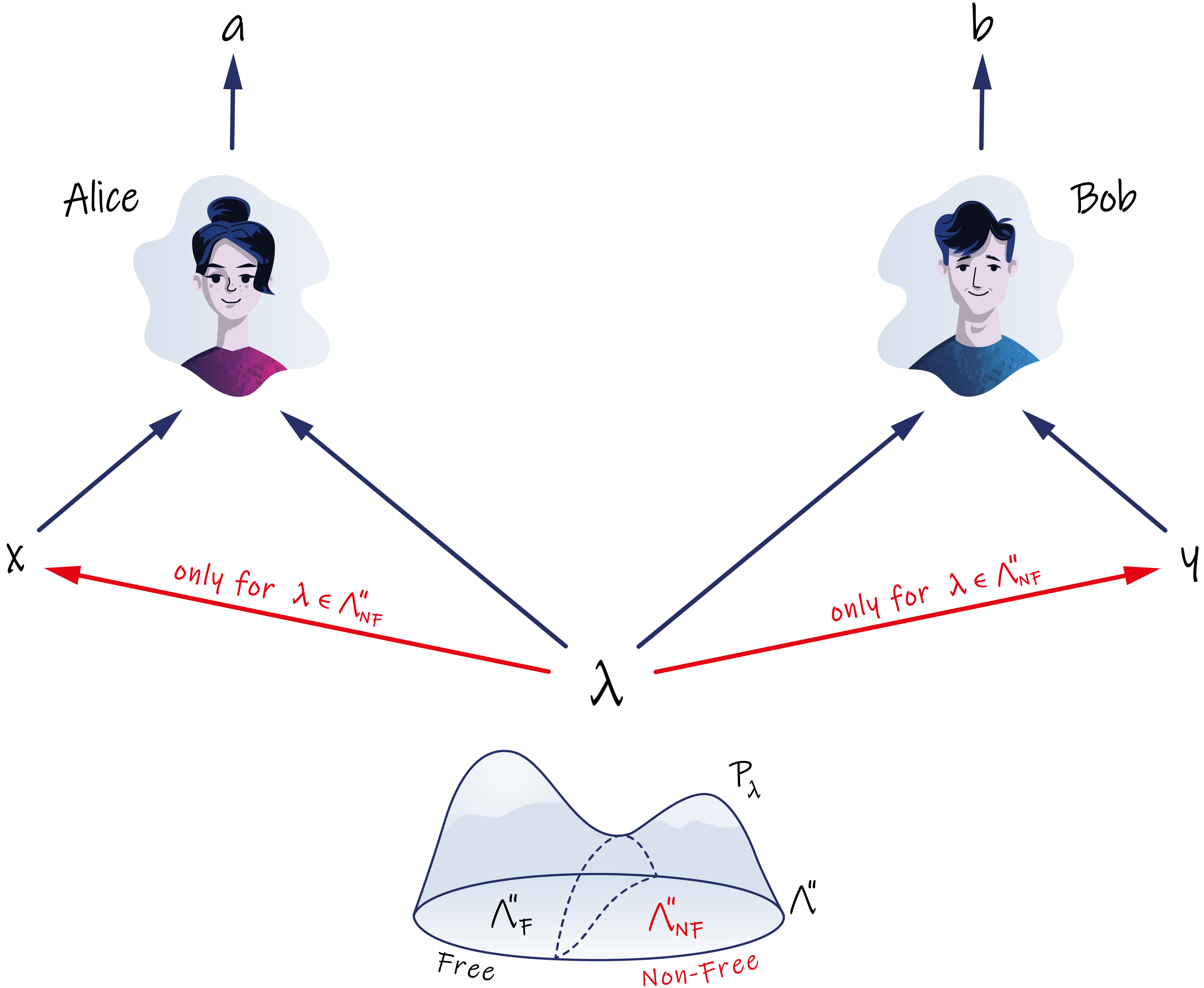
Figure 3: Causal model with some freedom of choice (rigging). In a Bell scenario, with locality assumption, correlations between the outcomes on Alice and Bob’s side can be explained by a common cause affecting choice or not (the latter implies freedom of choice). In any causal model the space of hidden variables (representing common causes) splits into two disjoint parts $\Lambda^{\prime\prime}=\Lambda^{\prime\prime}_{\scriptscriptstyle F}\cup\Lambda^{\prime\prime}_{\scriptscriptstyle NF}$ distinguished by whether, for a given $\lambda\in\Lambda^{\prime\prime}$, the choice is free or not, Eqs. (15). Then, the parties enjoy freedom of choice only on the trials when $\lambda\in\Lambda^{\prime\prime}_{\scriptscriptstyle F}$, which happens with a frequency equal to the probability accumulated over subset $\Lambda^{\prime\prime}_{\scriptscriptstyle F}$, i.e. ${{Prob}}\,(\lambda\in\Lambda^{\prime\prime}_{\scriptscriptstyle F})\,\equiv\,\sum_{\scriptscriptstyle\lambda\in\Lambda^{\prime\prime}_{F}}P_{\scriptscriptstyle\lambda}$.

The crucial point is the distinction between local vs non-local as well as free vs non-free situations in the individual runs of the experiment modelled by Eq. (6). This means that each condition Eq. (8) and Eq. (9) should be considered separately for each $\lambda\in\Lambda$, i.e. whenever the respective condition does not hold for a given $\lambda$ the assumption fails on the corresponding experimental trials. Such a distinction leads to a natural splitting of the underlying HV space into two unique partitions $\Lambda=\Lambda_{\scriptscriptstyle L}\cup\Lambda_{\scriptscriptstyle NL}$ and $\Lambda=\Lambda_{\scriptscriptstyle F}\cup\Lambda_{\scriptscriptstyle NF}$. The first one divides $\Lambda$ by the locality property

$$\begin{array}[]{lcl}\lambda\in\Lambda_{\scriptscriptstyle L}&\ \Leftrightarrow&\text{Eq.\leavevmode\nobreak\ (\ref{factorisation})}\ \ \text{holds for {all} $x,y\in\mathfrak{M}$}\,,\vspace{0.1cm}\\ \lambda\in\Lambda_{\scriptscriptstyle NL}&\ \Leftrightarrow&\text{Eq.\leavevmode\nobreak\ (\ref{factorisation})}\ \ \text{fails for {some} $x,y\in\mathfrak{M}$}\,,\end{array}$$ (12)

while the second one divides $\Lambda$ by the free choice property

$$\begin{array}[]{lcl}\lambda\in\Lambda_{\scriptscriptstyle F}&\ \Leftrightarrow&\text{Eq.\leavevmode\nobreak\ (\ref{free-choice})}\ \ \text{holds for {all} $x,y\in\mathfrak{M}$}\,,\vspace{0.1cm}\\ \lambda\in\Lambda_{\scriptscriptstyle NF}&\ \Leftrightarrow&\text{Eq.\leavevmode\nobreak\ (\ref{free-choice})}\ \ \text{fails for {some} $x,y\in\mathfrak{M}$}\,.\end{array}$$ (15)

Figs. 2 and 3 illustrate the causal structures for two extreme cases: FHV and LHV models (in general built on different HV spaces $\Lambda^{\prime}$ and $\Lambda^{\prime\prime}$). The first one grants full freedom of choice ($\Lambda^{\prime}=\Lambda^{\prime}_{\scriptscriptstyle F}$) while allowing for partial violation of locality ($\Lambda^{\prime}\supset\Lambda^{\prime}_{\scriptscriptstyle L}$). The second one retains full locality ($\Lambda^{\prime\prime}=\Lambda^{\prime\prime}_{\scriptscriptstyle L}$) while admitting some violation of free choice ($\Lambda^{\prime\prime}\supset\Lambda^{\prime\prime}_{\scriptscriptstyle F}$).

Thus, for a given experimental trial (with $\lambda\in\Lambda$ fixed) the constraints in Eqs. (12) and (15) indicate, respectively, whether some non-local influence between the parties takes place ($\lambda\in\Lambda_{\scriptscriptstyle NL}$) and whether some influence from the past on the measurement settings occurs ($\lambda\in\Lambda_{\scriptscriptstyle NF}$). In other words, in a hypothetical simulation scenario these possibilities correspond to, respectively, communication or rigging measurement settings. How often this has to happen depends on the distribution $P_{\scriptscriptstyle\lambda}$. This picture lends itself to quantifying the degree of locality and freedom choice in a given HV model.

Remark 1.

For a given HV model ($\star$ ‣ Causal models, locality and free choice) locality is measured by $\textsl{{Prob}}\,(\lambda\in\Lambda_{\scriptscriptstyle L})\,\equiv\,\sum_{\scriptscriptstyle\lambda\in\Lambda_{L}}P_{\scriptscriptstyle\lambda}$, and similarly freedom of choice is measured by $\textsl{{Prob}}\,(\lambda\in\Lambda_{\scriptscriptstyle F})\,\equiv\,\sum_{\scriptscriptstyle\lambda\in\Lambda_{F}}P_{\scriptscriptstyle\lambda}$.

This remark captures the intuition of measuring locality and freedom of choice by considering the proportion of trials when the respective property is maintained across the whole experimental ensemble. We note that this quantity is model-dependent, since it is a property of a particular HV model adopted to explain some given experimental statistics $\{P_{\scriptscriptstyle ab|xy}\}_{\scriptscriptstyle xy}$ (including the distribution of measurement settings $P_{\scriptscriptstyle xy}$, cf. Eq. (7)).

The concepts just introduced allow a precise expression for the informal definitions ($\scriptstyle\spadesuit$ ‣ Bell experiment and Fine’s theorem) and ($\scriptstyle\clubsuit$ ‣ Bell experiment and Fine’s theorem) given above.

Definition 1.

For a given behaviour $\{P_{\scriptscriptstyle ab|xy}\}_{\scriptscriptstyle xy}$ the measure of locality $\mu_{\scriptscriptstyle L}$ and freedom of choice $\mu_{\scriptscriptstyle F}$ are defined as

$$\mu_{\scriptscriptstyle L}\ :=\ \min_{\scriptscriptstyle P_{\scriptscriptstyle xy}}\,\max_{\scriptscriptstyle FHV}\sum_{\scriptscriptstyle\lambda\in\Lambda_{L}}P_{\scriptscriptstyle\lambda}\,\,,$$ (16)

$$\mu_{\scriptscriptstyle F}\ :=\ \min_{\scriptscriptstyle P_{\scriptscriptstyle xy}}\,\max_{\scriptscriptstyle LHV}\sum_{\scriptscriptstyle\lambda\in\Lambda_{F}}P_{\scriptscriptstyle\lambda}\,\,,$$ (17)

where the maxima are taken respectively over all hidden variable models with freedom of choice (FHV) or all local hidden variable models (LHV) simulating given behaviour $\{P_{\scriptscriptstyle ab|xy}\}_{\scriptscriptstyle xy}$, with a fixed distribution of settings $P_{\scriptscriptstyle xy}$ , minimized over any choice of the latter.

This definition follows the intuition of, respectively, locality or free choice as properties that can be relaxed only to the extent that is required to maintain the other assumption in every experimental situation (i.e., for any distribution of measurement settings $P_{\scriptscriptstyle xy}$). Formally, the measures $\mu_{\scriptscriptstyle L}$ and $\mu_{\scriptscriptstyle F}$ count the maximal frequency of, respectively, local or free choice events optimised over all protocols simulating $\{P_{\scriptscriptstyle ab|xy}\}_{\scriptscriptstyle xy}$ without violating of the other assumption, cf. Remark 1. The minimum over all $P_{\scriptscriptstyle xy}$ amounts to the worst case scenario, which takes into account the possibility that $P_{\scriptscriptstyle xy}$ is a priori unspecified (i.e., this amount of freedom is enough to simulate an experiment with any arbitrary choice of distribution $P_{\scriptscriptstyle xy}$ in compliance with Eq. (7)).

At first glance, even if conceptually appropriate, such a definition might seem too general to provide a manageable notion, due to the range of experimental scenarios that need to be taken into account (i.e. arbitrariness of $P_{\scriptscriptstyle xy}$). However, the situation considerably simplifies because of the following lemma (see Methods section for further discussion and proof). This lemma also provides additional support for Definition 1.

Lemma 1.

In both Eqs. (16) and (17) in Definition 1 the first minimum can be omitted, i.e. we have

$$\mu_{\scriptscriptstyle L}\ =\ \max_{\scriptscriptstyle FHV}\sum_{\scriptscriptstyle\lambda\in\Lambda_{L}}P_{\scriptscriptstyle\lambda}\,\,,$$ (18)

$$\mu_{\scriptscriptstyle F}\ =\ \max_{\scriptscriptstyle LHV}\sum_{\scriptscriptstyle\lambda\in\Lambda_{F}}P_{\scriptscriptstyle\lambda}\,\,,$$ (19)

where the respective maxima are taken for some fixed nontrivial distribution $P_{\scriptscriptstyle xy}$ (i.e., the expression is insensitive to this choice provided all settings are probed, $P_{\scriptscriptstyle xy}\neq 0$ for all $x,y$).

It is in this way that the present measure of locality $\mu_{\scriptscriptstyle L}$ extends the notion of local fraction (27, 28, 29, 30, 31, 32) to arbitrary experimental behaviour $\{P_{\scriptscriptstyle ab|xy}\}_{\scriptscriptstyle xy}$. Remarkably, the twin concept, which is the measure of free choice $\mu_{\scriptscriptstyle F}$ has not been considered at all. Perhaps the reason for this omission is the issue of arbitrariness of the distribution $P_{\scriptscriptstyle xy}$, for which there are non-trivial constraints when freedom of choice is violated (note that for the measure $\mu_{\scriptscriptstyle L}$ this problem does not occur). Those concerns can be dismissed only after the proper treatment in Lemma 1. This allows a so defined measure of freedom $\mu_{\scriptscriptstyle F}$ on a par with the more familiar measure of locality $\mu_{\scriptscriptstyle L}$.

So far the concepts of violation of locality and freedom of choice, and the corresponding measures $\mu_{\scriptscriptstyle L}$ and $\mu_{\scriptscriptstyle F}$, have been kept separate. This is expected given their disparate character. First, each concept plays a different role in the description of an experiment and hence offers a different explanation for any observed correlations, this is, direct influence (communication during the experiment) vs measurement dependence (employing common past for rigging measurement settings). Second, on the level of causal modelling those assumptions are expressed differently, Eq. (8) vs Eq. (9). Third, violating free choice gives rise to subtle issues regarding constraints on the distribution of settings $P_{\scriptscriptstyle xy}$ (as noted, these concerns are addressed in Lemma 1).

Having brought all those issues to the spotlight, it is surprising that the assumption of locality and free choice are intrinsically connected. We now present the key result in this paper showing the exchangeability of both concepts, while maintaining the same degree of locality and freedom of choice so defined. It holds for any number of settings $x,y\in\mathfrak{M}=\{0,1,...\,,M\}$ (see Methods for the proof).

Theorem 1.

For a given behaviour $\{P_{\scriptscriptstyle ab|xy}\}_{\scriptscriptstyle xy}$ the degree of locality and freedom of choice are the same, i.e. both measures in Definition 1 coincide $\mu_{\scriptscriptstyle L}=\mu_{\scriptscriptstyle F}$.

This is a general structural theorem about causal modelling of a given behaviour $\{P_{\scriptscriptstyle ab|xy}\}_{\scriptscriptstyle xy}$. It means that the resources measured by the frequency of causal interventions of either sort, required to explain an experimental statistics, are equally costly. Thus, as far as the statistics is concerned, causal explanations resorting either to violation of locality or free choice (or measurement dependence) should be kept on an equal footing. Preference should be guided by a better understanding of a particular situation (design of the experiment as well as ontological commitments in its description).

Let us emphasise two features of Theorem 1. First, this is a theory-independent result in the sense that it applies directly to experimental statistics irrespective of the design or theoretical framework behind the experiment (with the quantum predictions being just one example). Second, the connection between those two seemingly disparate quantities $\mu_{\scriptscriptstyle L}$ and $\mu_{\scriptscriptstyle F}$ has a practical advantage: knowledge of one suffices to compute the other. Both features are illustrated by the following results.

Non-signalling behaviour with binary settings

Consider the case of Bell’s experiment with only two measurement settings on each side $x,y\in\mathfrak{M}=\{0,1\}$. Let us recall that non-signalling of some given behaviour $\{P_{\scriptscriptstyle ab|xy}\}_{\scriptscriptstyle xy}$ means that Alice cannot infer Bob’s measurement setting (whether it is $y=0$ or $1$) from the statistics on her side alone, i.e.

$$P_{\scriptscriptstyle a|x0}\ =\ \sum_{\scriptscriptstyle b}P_{\scriptscriptstyle ab|x0}\ =\ \sum_{\scriptscriptstyle b}P_{\scriptscriptstyle ab|x1}\ =\ P_{\scriptscriptstyle a|x1}\quad\text{ for all $a,x$}\,,$$ (20)

and similarly on Bob’s side (whether Alice chooses $x=0$ or $1$), i.e.

$$P_{\scriptscriptstyle b|0y}\ =\ \sum_{\scriptscriptstyle a}P_{\scriptscriptstyle ab|0y}\ =\ \sum_{\scriptscriptstyle a}P_{\scriptscriptstyle ab|1y}\ =\ P_{\scriptscriptstyle b|1y}\quad\text{ for all $b,y$}\,.$$ (21)

Now we can state another result which explicitly computes both measures $\mu_{\scriptscriptstyle L}$ and $\mu_{\scriptscriptstyle F}$ in a surprisingly simple form (see Methods for the proof).

Theorem 2.

For a given non-signalling behaviour $\{P_{\scriptscriptstyle ab|xy}\}_{\scriptscriptstyle xy}$ with binary settings $x,y\in\mathfrak{M}=\{0,1\}$ both measures of locality $\mu_{\scriptscriptstyle L}$ and free choice $\mu_{\scriptscriptstyle F}$ from Definition 1 are equal to

$$\mu_{\scriptscriptstyle L}\ =\ \mu_{\scriptscriptstyle F}\ =\ \left\{\begin{array}[]{lll}\tfrac{1}{2}(4-S_{\scriptscriptstyle max})\,,&&\text{if $S_{\scriptscriptstyle max}>2$\,,}\vspace{0.15cm}\\ 1\,,&&\text{otherwise\,,}\end{array}\right.$$ (24)

where $S_{\scriptscriptstyle max}=\max\,\{|S_{\scriptscriptstyle i}|:i=1,...\,,4\}$ is the maximum absolute value of the four CHSH expressions in Eqs. (2)-(5).

We thus obtain a systematic method for assessing the degree of locality and free choice directly from the observed statistics $\{P_{\scriptscriptstyle ab|xy}\}_{\scriptscriptstyle xy}$ without reference to the specifics of the experiment (the only requirement is non-signalling of the observed distributions). In this sense, this is a general theory-independent statement.

Overall, Theorem 2 allows an interpretation of the amount of violation of the CHSH inequalities in Bell-type experiments as a fraction of trials violating locality (granted freedom of choice) or equivalently trials without freedom of choice (given locality).

The quantum case: Binary settings and beyond

Let us restrict our attention to the special case of the quantum statistics. Notably, various aspects of non-locality have been extensively researched in relation to the quantum-mechanical predictions, see (4, 5) for a review. This includes the notion of local fraction (27, 28, 29, 30, 31, 32), which is the same as measure $\mu_{\scriptscriptstyle L}$ here defined for a general behaviour $\{P_{\scriptscriptstyle ab|xy}\}_{\scriptscriptstyle xy}$. As noted, it may be thus surprising that the equally natural measure of freedom $\mu_{\scriptscriptstyle F}$ has not been explored. Theorem 1 bridges the gap between those two seemingly disparate notions: there is no actual need for separate study. We next review some crucial results for the local fraction in the quantum-mechanical framework, which allows us to make similar statements for the measure of freedom $\mu_{\scriptscriptstyle F}$.

We first observe that Theorem 2 can be readily applied to the quantum-mechanical statistics (where non-signalling holds). In a Bell experiment, quantum probabilities obtain through the standard formula $P_{\scriptscriptstyle ab|xy}=Tr\,[\,\rho\,\mathbb{P}_{\scriptscriptstyle x}^{\scriptscriptstyle a}\otimes\mathbb{P}_{\scriptscriptstyle y}^{\scriptscriptstyle b}\,]$ where $\rho$ is a (bipartite) mixed state with two PVMs $\{\mathbb{P}_{\scriptscriptstyle x}^{\scriptscriptstyle a=\pm 1}\}$ and $\{\mathbb{P}_{\scriptscriptstyle y}^{\scriptscriptstyle b=\pm 1}\}$ representing Alice and Bob’s choice of measurement settings $x,y\in\mathfrak{M}=\{0,1\}$. Calculating the CHSH expressions Eqs. (2)-(5) in each particular case is straightforward, which gives explicitly the expression for both measures $\mu_{\scriptscriptstyle L}$ and $\mu_{\scriptscriptstyle F}$ via Eq. (24). The result of special significance concerns the famous Tsirelson bound $S_{\scriptscriptstyle max}^{\scriptscriptstyle QM}=2\sqrt{2}$ for the maximal violation of the CHSH inequalities in quantum mechanics (47). By virtue of Theorem 2, this means that in order to locally recover the quantum predictions in a Bell experiment with two settings, Alice and Bob can enjoy freedom of choice in the worst case, at most, with a fraction $\mu_{\scriptscriptstyle F}=2-\sqrt{2}\approx 0.59$ of all trials (corresponding to the choice of measurements on a maximally entangled state that saturate the Tsirelson bound). Clearly, the same applies to local fraction $\mu_{\scriptscriptstyle L}$ in a two-setting scenario.

Interestingly, relaxing the constraint on the number of settings for Alice and Bob’s measurements $x,y\in\mathfrak{M}=\{1,\,2,\,3,...\,,M\}$ the quantum statistics forces us to further constrain, respectively, locality or free choice. The case of local fraction $\mu_{\scriptscriptstyle L}$ with arbitrary number of settings $M\rightarrow\infty$ has been thoroughly investigated for statistics generated by quantum states. Let us refer to two interesting results in the literature on local fraction $\mu_{\scriptscriptstyle L}$ which readily translate via Theorem 1 to the measure of freedom $\mu_{\scriptscriptstyle F}$. The first one concerns the statistics of a maximally entangled state, cf. (27, 29) (see SI Appendix for a direct proof).

Theorem 3.

For every local hidden variable (LHV) model that explains the statistics of a Bell experiment for a maximally entangled state the amount of free choice tends to zero with increasing number of measurement settings $M$, i.e. $\mu_{\scriptscriptstyle F}\xymatrix{\ar[r]_{M\,\rightarrow\,\infty\atop}&}0\,$ .

Apparently, for less entangled states the amount of freedom increases, reaching the maximal value $\mu_{\scriptscriptstyle F}=1$ for separable states. This is a consequence of the result in (32), which explicitly computes the local fraction $\mu_{\scriptscriptstyle L}$ for all pure two-qubit states. Stated for measure $\mu_{\scriptscriptstyle F}$ this takes the following form.

Theorem 4.

For a pure two-qubit state, which by appropriate choice of the basis can always be written in the form $\ket{\psi}=\cos\tfrac{\theta}{2}\ket{00}+\sin\tfrac{\theta}{2}\ket{11}$ with $\theta\in[0,\tfrac{\pi}{2}]$, the amount of freedom is equal $\mu_{\scriptscriptstyle F}=\cos\,\theta$, whatever the choice and number of settings on Alice and Bob’s side.

Note that both Theorem 3 and Theorem 4 assume a specific form of behaviour $\{P_{\scriptscriptstyle ab|xy}\}_{\scriptscriptstyle xy}$ as obtained by the rules of quantum theory. The theorems should be contrasted with Theorem 2 which is a theory-independent statement, not limited to a particular theoretical framework.

Discussion

The ingenuity of Bell’s theorem lies in the fundamental nature of the premises from which the result is derived. Within the standard causal (or realist) approach, it is hard to assume less about two agents than having free choice and their systems being localised in space. Yet in some experiments nature refutes the possibility that both assumptions are concurrently true (8, 9, 10, 11, 12, 13, 14, 15). It is not easy to reject either one of them without carefully rethinking the role of observers and how cause-and-effect manifests in the world. Our objective in this paper is this: instead of pondering the question of how this could be possible, we ask about the extent to which a given assumption has to be relaxed in order to maintain the other. Expressed more colloquially, it is natural for a realist to ask what is the cost of trading one concept for the other: Is it possible to save free choice by giving up on some locality? Or, maybe is it better to forego a modicum of free choice in exchange for locality? These questions can be compared on equal footing by computing a proportion of trials across the whole experimental ensemble in which a given assumption must fail, when the other holds at all times. Surprisingly, the answer can be obtained by looking at the observed statistics alone (avoiding the specifics of the experimental setup). The first question was formulated in the quantum-mechanical context by Elitzur, Popescu and Rohrlich (27) who introduced the notion of local fraction further elaborated in (29, 30, 31, 32) (see (28) for an early indication of these ideas). Here, we generalise this notion to arbitrary experimental statistics (see also (33)). Furthermore, we answer the second question by adopting a similar approach to measuring the amount of free choice (which by analogy may be called free fraction). The first main result, Theorem 1, compares such defined measures in the general case (arbitrary statistics with any number of settings), showing that both assumptions are equally costly. This demonstrates a deeper symmetry between locality and free choice, which may come as a surprise, given our intuition of a profound difference in the role these concepts play in the description of an experiment.

In this paper, the notions of locality and free choice are understood in the usual sense required to derive Bell’s theorem (6, 22). They are expressed in the standard causal model framework (which subsumes realism) as unambiguous yes-no criteria for each experimental trial (i.e. when all past variables are fixed), determining whether there is a causal link between certain variables in a model (without pondering its exact nature). The measures $\mu_{\scriptscriptstyle L}$ and $\mu_{\scriptscriptstyle F}$ count the fraction of trials when such a connection needs to be established, breaking locality or free choice respectively, in order to explain the observed statistics. This problem is prior to a discussion of how this actually occurs, which is particularly relevant when the exact nature of the phenomenon under study is obscured. Theorem 1 shows no intrinsic reason for a realist to favour one assumption vs the other. The minimal frequency of the required causal influences of either sort, measured by $\mu_{\scriptscriptstyle L}$ and $\mu_{\scriptscriptstyle F}$, is exactly the same. Notably, this is a general result which holds for any behaviour $\{P_{\scriptscriptstyle ab|xy}\}_{\scriptscriptstyle xy}$. What remains is explicit calculation of those measures for a given experimental statistics.

The second main result, Theorem 2, evaluates both measures $\mu_{\scriptscriptstyle L}$ and $\mu_{\scriptscriptstyle F}$ for any non-signalling behaviour in a Bell experiment with two outcomes and two settings. It provides a direct interpretation to the amount of violation of the CHSH inequalities (43). The key motivation behind this result is that the degree by which the inequalities are violated has not been given tangible interpretation so far, beyond its use as a binary test of whether the inequalities are obeyed or not in study of Bell non-locality. Furthermore, Theorem 2 has the advantage of being theory-independent in the sense of being applicable to the experimental statistics regardless of its theoretical origin (i.e., beyond the quantum-mechanical framework). This makes it suitable for quantitative assessment of the degree of locality and free choice across different experimental situations, with prospective applications beyond physics, e.g. in neuroscience, cognitive psychology, social sciences or finance (48, 49, 50, 51, 52).

We also state two results, Theorem 3 and Theorem 4, for the measure of free choice $\mu_{\scriptscriptstyle F}$ in the case of the quantum statistics generated by the pure two-qubit states. Both are direct translation, via Theorem 1, of the corresponding results for the local fraction $\mu_{\scriptscriptstyle L}$ (27, 28, 29, 30, 31, 32).

It is worth noting a related idea of quantifying non-locality through the amount of information transmitted between the parties that is required to reproduce quantum correlations (under free choice assumption). Together with the development of the specific models (53, 54, 55, 56, 57), this has led to various results regarding communication complexity in the quantum realm (58). However, in this paper we take a different perspective on measuring non-locality by changing the question from "how much" to "how often" communication needs to be established between the parties to simulate given correlations. Theorem 2 gives the exact bound in the case of non-signalling statistics in the two-setting and two-outcome Bell experiment. In the quantum case, such a simulation requires communication in at least 41 % of trials (because of Tsirelson’s bound (47)) and for maximally entangled states increases to 100 % of trials when the number of settings is arbitrary (cf. Theorems 3 and 4).

Natural as it may seem, the idea of measuring freedom of choice by measure $\mu_{\scriptscriptstyle F}$ has not been developed in the literature. The reason for this omission can be traced to the conceptual and technical issues with handling arbitrariness of the distribution of settings $P_{\scriptscriptstyle xy}$. Those concerns are properly addressed in the present paper with Lemma 1, which considerably simplifies and supports Definition 1. We note that various measures have been developed as a means of quantifying freedom of choice (or measurement independence, as it is sometimes called). They include maximal distance between distributions (35, 37), mutual information (38, 42) or measurement dependent locality (39, 40, 41). Furthermore, some explicit models simulating correlations in a singlet state with various degrees of measurement dependence have been proposed (34, 36) and analysed (e.g. see (42) for comparison of causal vs retrocausal models). However, these attempts depart from the original understanding of the free choice as introduced by Bell (6, 22) (strict independence of choice from anything in the past) in favour of more sophisticated information-theoretic accounts. Notably, the proposed measure of free choice builds on the Bell’s original framework assessing the maximal frequency with which such a freedom can be retained in a model strictly consistent with locality. It thus benefits from a direct interpretation within the established causal framework of Bell inequalities and has a clear-cut operational meaning.

Regarding Theorem 3, which rules out any freedom of choice so defined, it is interesting to take an adversarial perspective on the problem of free choice in relation to quantum cryptography and device independent certification (59, 60). In this narrative an eavesdropper controls the devices trying to simulate the quantum statistics of a Bell test, which is impossible as long as the parties enjoy freedom of choice. However, any breach of the latter, i.e. control of measurement settings, shifts the balance in favour of the eavesdropper in her malicious task. Taking the view that any causal influence comes with a cost or danger of being uncovered there are two diverging strategies that reduce the cost/risk to be considered: (a) resort to the use of control of choice as seldom as possible during the experiment, or (b) minimise the intensity of each act of control. Theorem 3 completely rules out the first possibility when simulating quantum statistics, i.e., the eavesdropper needs to manipulate both settings on each trial in order to simulate the quantum statistics. The question about the intensity of the control is left open in our discussion, but amenable to information-theoretic methods (35, 36, 35, 37, 38, 39, 40, 41, 42). This gives additional security criteria for quantum cryptography and device independent certification by forcing the eavesdropper to a more challenging sort of attack (not only can she not miss a trial, but the control has to be subtle enough).

We remark that the main Theorem 1 readily extends to the case of larger number of parties and outcomes $\{P_{\scriptscriptstyle abc...|xyz...}\}_{\scriptscriptstyle xyz...}$. This should be also possible for Theorem 2 when characterisation of the local polytope is known, cf. (61, 62, 63, 64, 65, 66, 67). Yet another valuable avenue for research in that case consists of completing the analysis to include signalling scenarios (68, 69). As for the quantum case, we considered the simplest Bell-type scenario with two parties involved in the experiment, but extensions may prove even more surprising (see (5) for a technical review of the vast field of Bell non-locality). In particular, in three-party scenarios the methods discussed presently can be used to eliminate freedom of choice already for two settings per party sharing the GHZ state (cf. Mermin inequalities which saturate in that case (70)). We should also mention an intriguing result (71) for a triangle quantum network in which non-locality can be proved with all measurements fixed. Remarkably, there is nothing to choose in that setup, but there is another assumption of preparation independence which plays a crucial role in the argument.

In this paper we are trying to remain impartial as to which assumption — locality or free choice — is more important on the fundamental level. This is certainly a strongly debated subject in general, both among physicists and philosophers, with strong supporters on each side (16, 17, 18). As just one example depreciating the role of freedom of choice let us quote Albert Einstein: "Human beings, in their thinking, feeling and acting are not free agents but are as causally bound as the stars in their motion." As a counterbalance, it is hard to resist the objection that was eloquently stated by Nicolas Gisin (72): "But for me, the situation is very clear: not only does free will exist, but it is a prerequisite for science, philosophy, and our very ability to think rationally in a meaningful way." Without entering into this debate, we remark that both assumptions are interchangeable on a deeper level. Namely, for a given experimental statistics $\{P_{\scriptscriptstyle ab|xy}\}_{\scriptscriptstyle xy}$ in a Bell-type experiment the measure of locality $\mu_{\scriptscriptstyle L}$ and measure of free choice $\mu_{\scriptscriptstyle F}$ are exactly the same. This makes an even stronger case regarding the inherent impossibility of inferring causal structure from experimental statistics alone.

In order to facilitate the following discussion we begin with two technical lemmas. See SI Appendix for the proofs.

The first one holds for a Bell experiment with arbitrary number of settings $x,y\in\mathfrak{M}=\{1,\,2,\,3,...\,,M\}$.

Lemma 2.

For any behaviour $\{{P}_{\scriptscriptstyle ab|xy}\}_{\scriptscriptstyle xy}$ and distribution of settings $P_{\scriptscriptstyle xy}$ there exists a local hidden variable model (LHV) which fully violates the freedom of choice assumption. [i.e. if $\tilde{\Lambda}$ is the relevant HV space, then we have $\tilde{\Lambda}=\tilde{\Lambda}_{\scriptscriptstyle L}=\tilde{\Lambda}_{\scriptscriptstyle NF}$, cf. Eqs. (12) and (15))].

The second one concerns a Bell scenario with binary settings $x,y\in\mathfrak{M}=\{0,\,1\}$.

Lemma 3.

Each non-signalling behaviour $\{P_{\scriptscriptstyle ab|xy}\}_{\scriptscriptstyle xy}$ with binary settings $x,y\in\mathfrak{M}=\{0,\,1\}$ can be decomposed as a convex mixture of a local behaviour $\{\bar{P}_{\scriptscriptstyle ab|xy}\}_{\scriptscriptstyle xy}$ and a PR-box $\{\tilde{P}_{\scriptscriptstyle ab|xy}\}_{\scriptscriptstyle xy}$ in the form

$$P_{\scriptscriptstyle ab|xy}\ =\ p\cdot\bar{P}_{\scriptscriptstyle ab|xy}+(1-p)\cdot\tilde{P}_{\scriptscriptstyle ab|xy}\,,$$ (25)

with $p=\tfrac{1}{2}(4-S_{\scriptscriptstyle max})$ for all $x,y\in\{0,1\}$.

Recall that a PR-box (73) is a non-signalling behaviour for which one of the CHSH expressions in Eqs. (2)-(5) reaches the maximal algebraic bound of $|S_{\scriptscriptstyle i}|=4$. Here, local behaviour means existence of a LHV+FHV model of $\{\bar{P}_{\scriptscriptstyle ab|xy}\}_{\scriptscriptstyle xy}$ and $S_{\scriptscriptstyle max}=\max\,\{|S_{\scriptscriptstyle i}|:i=1,...\,,4\}$.

We are now ready to proceed with the proofs.

Proof of Lemma 1

Suppose we have a HV model ($\star$ ‣ Causal models, locality and free choice) of some behaviour $\{P_{\scriptscriptstyle ab|xy}\}_{\scriptscriptstyle xy}$ for some nontrivial distribution of settings ${P}_{\scriptscriptstyle xy}$. The latter obtains via Eq. (7) from the conditional probabilities ${P}_{\scriptscriptstyle xy|\lambda}$ which are related to probabilities specified by the model, ${P}_{\scriptscriptstyle\lambda|xy}$ and ${P}_{\scriptscriptstyle\lambda}$ , by the usual Bayes’ rule. The point at issue is whether a given HV model can simulate any other distribution of settings $\tilde{P}_{\scriptscriptstyle xy}$ via Eq. (7) by changing ${P}_{\scriptscriptstyle xy|\lambda}\leadsto\tilde{P}_{\scriptscriptstyle xy|\lambda}$ , while keeping the remaining components of the HV model ($\star$ ‣ Causal models, locality and free choice) intact. This requires consistency with Bayes’ rule, i.e.

$$\tilde{P}_{\scriptscriptstyle xy|\lambda}\ =\ \tfrac{{P}_{\scriptscriptstyle\lambda|xy}\cdot\,\tilde{P}_{xy}}{{P}_{\scriptscriptstyle\lambda}}\,,$$ (26)

which should be a well-defined probability distribution for each $\lambda$. Since distributions ${P}_{\scriptscriptstyle\lambda|xy}$ and ${P}_{\scriptscriptstyle\lambda}$ are fixed by the HV model ($\star$ ‣ Causal models, locality and free choice), then the distribution of settings $\tilde{P}_{\scriptscriptstyle xy}$ is arbitrary as long as the expression in Eq. (26) is less then 1 for each $\lambda\in\Lambda$ (normalisation is trivially fulfilled). Now, whenever freedom of choice from Eq. (9) holds, this condition is always satisfied, and hence such a HV model can be trivially adjusted for any distribution $\tilde{P}_{\scriptscriptstyle xy}$ (by redefining $\tilde{P}_{\scriptscriptstyle xy|\lambda}:=\tilde{P}_{\scriptscriptstyle xy}$ in compliance with Eq. (26), and keeping all the remaining components of the HV model ($\star$ ‣ Causal models, locality and free choice) unchanged). Of course, for FHV models in the definition of $\mu_{\scriptscriptstyle L}$ in Eq. (16) this is the case, which thus entails the simpler expression for $\mu_{\scriptscriptstyle L}$ in Eq. (18).

Clearly, such a simple argument falls apart for models without freedom of choice, like those in the definition of $\mu_{\scriptscriptstyle F}$ in Eq. (17), when ${P}_{\scriptscriptstyle\lambda|xy}$ and ${P}_{\scriptscriptstyle\lambda}$ do not cancel out and the probability in Eq. (26) may be ill-defined. In that case, some deeper intervention into the model is required as shown below.

Let us take some LHV model ($\star$ ‣ Causal models, locality and free choice) simulating a given behaviour $\{P_{\scriptscriptstyle ab|xy}\}_{\scriptscriptstyle xy}$ with nontrivial distribution of settings $P_{\scriptscriptstyle xy}$. Then the related HV space decomposes as $\Lambda=\Lambda_{\scriptscriptstyle F}\uplus\Lambda_{\scriptscriptstyle NF}$ and the degree of freedom is measured by $p_{\scriptscriptstyle F}:=\sum_{\scriptscriptstyle\lambda\in\Lambda_{F}}P_{\scriptscriptstyle\lambda}$ , cf. Remark 1. Now, consider a restriction of the model to the respective subspaces $\Lambda_{\scriptscriptstyle F}$ and $\Lambda_{\scriptscriptstyle NF}$ which amounts to the following rescaling

$$P_{\scriptscriptstyle\lambda}^{\scriptscriptstyle F}\ :=\ \tfrac{1}{p_{\scriptscriptstyle F}}\,P_{\scriptscriptstyle\lambda}\,,\quad P_{\scriptscriptstyle\lambda|xy}^{\scriptscriptstyle F}\ :=\ \tfrac{1}{p_{\scriptscriptstyle F}}\,P_{\scriptscriptstyle\lambda|xy}\,,\quad P_{\scriptscriptstyle ab|xy\lambda}^{\scriptscriptstyle F}\ :=\ P_{\scriptscriptstyle ab|xy\lambda}\,,$$ (27)

for $\lambda\in\Lambda_{\scriptscriptstyle F}$, and similarly

$$P_{\scriptscriptstyle\lambda}^{\scriptscriptstyle NF}\ :=\ \tfrac{1}{1-p_{\scriptscriptstyle F}}\,P_{\scriptscriptstyle\lambda}\,,\quad P_{\scriptscriptstyle\lambda|xy}^{\scriptscriptstyle NF}\ :=\ \tfrac{1}{1-p_{\scriptscriptstyle F}}\,P_{\scriptscriptstyle\lambda|xy}\,,\quad P_{\scriptscriptstyle ab|xy\lambda}^{\scriptscriptstyle NF}\ :=\ P_{\scriptscriptstyle ab|xy\lambda}\,,$$ (28)

for $\lambda\in\Lambda_{\scriptscriptstyle NF}$. Both are LHV models with marginals

$$P_{\scriptscriptstyle ab|xy}^{\scriptscriptstyle F}\ =\ \sum_{\scriptscriptstyle\lambda\in\Lambda_{\scriptscriptstyle F}}\,P_{\scriptscriptstyle ab|xy\lambda}^{\scriptscriptstyle F}\cdot P_{\scriptscriptstyle\lambda|xy}^{\scriptscriptstyle F}\,,$$ (29)

$$P_{\scriptscriptstyle ab|xy}^{\scriptscriptstyle NF}\ =\ \sum_{\scriptscriptstyle\lambda\in\Lambda_{\scriptscriptstyle NF}}\!P_{\scriptscriptstyle ab|xy\lambda}^{\scriptscriptstyle NF}\cdot P_{\scriptscriptstyle\lambda|xy}^{\scriptscriptstyle NF}\,,$$ (30)

which provide a convex decomposition of the original behaviour $\{P_{\scriptscriptstyle ab|xy}\}_{\scriptscriptstyle xy}$ , i.e.

$$P_{\scriptscriptstyle ab|xy}\ =\ p_{\scriptscriptstyle F}\cdot P_{\scriptscriptstyle ab|xy}^{\scriptscriptstyle F}+(1-p_{\scriptscriptstyle F})\cdot P_{\scriptscriptstyle ab|xy}^{\scriptscriptstyle NF}\,.$$ (31)

The crucial point is a careful adjustment of these two models to recover some arbitrary distribution of settings $\tilde{P}_{\scriptscriptstyle xy}$, while maintaining the respective marginals Eqs. (29) and (30). For the first one (restriction to $\Lambda_{\scriptscriptstyle F}$) the situation is trivial as explained above: since it is a FHV model, then it suffice to redefine $\tilde{P}_{\scriptscriptstyle xy|\lambda}^{\scriptscriptstyle F}:=\tilde{P}_{\scriptscriptstyle xy}$ (in compliance with Eq. (26)) and leave all rest intact. As for the second one (restriction to $\Lambda_{\scriptscriptstyle NF}$), we can use Lemma 2 for constructing another HV space $\tilde{\Lambda}_{\scriptscriptstyle NF}$ with a LHV model without any free choice, that simulates behaviour $\{P_{\scriptscriptstyle ab|xy}^{\scriptscriptstyle NF}\}_{\scriptscriptstyle xy}$ with the required distribution of settings $\tilde{P}_{\scriptscriptstyle xy}$. Then, such modified models can be stitched back together on the compound HV space $\tilde{\Lambda}:=\Lambda_{\scriptscriptstyle F}\uplus\tilde{\Lambda}_{\scriptscriptstyle NF}$ with respective weights $p_{\scriptscriptstyle F}$ and $1-p_{\scriptscriptstyle F}$. This guarantees reconstruction of the original behaviour $\{P_{\scriptscriptstyle ab|xy}\}_{\scriptscriptstyle xy}$ (see Eq. (31)) with the new distribution of settings $\tilde{P}_{\scriptscriptstyle xy}$. The model is local and has the same degree of freedom equal to $p_{\scriptscriptstyle F}$ (the first component has full freedom of choice, while in the second one it is entirely missing).

The above construction shows that for every LHV model of some behaviour $\{P_{\scriptscriptstyle ab|xy}\}_{\scriptscriptstyle xy}$ there is always another one adjusted for any other distribution of settings $\tilde{P}_{\scriptscriptstyle xy}$ with the same degree of freedom. This justifies the simpler expression for $\mu_{\scriptscriptstyle F}$ in Eq. (19) and hence concludes the proof of Lemma 1.

Proof of Theorem 1

Note that Lemma 1 Eqs. (18) and (19) can be taken as a definition of measures $\mu_{\scriptscriptstyle L}$ and $\mu_{\scriptscriptstyle F}$. This is very convenient, since it allows a discussion free from any concerns about the distribution of settings $P_{xy}$ (this is particularly relevant in the case of $\mu_{\scriptscriptstyle F}$ as explained above).

It is instructive to observe that the calculation of both measures $\mu_{\scriptscriptstyle L}$ and $\mu_{\scriptscriptstyle F}$ can be succinctly formulated as a convex optimisation problem. Suppose, we can decompose some given behaviour $\{P_{\scriptscriptstyle ab|xy}\}_{\scriptscriptstyle xy}$ as a mixture

$$P_{\scriptscriptstyle ab|xy}\ =\ p_{\scriptscriptstyle L}\cdot P_{\scriptscriptstyle ab|xy}^{\scriptscriptstyle L}+(1-p_{\scriptscriptstyle L})\cdot P_{\scriptscriptstyle ab|xy}^{\scriptscriptstyle NL}\,,$$ (32)

where $\{P_{\scriptscriptstyle ab|xy}^{\scriptscriptstyle L}\}_{\scriptscriptstyle xy}$ is a local behaviour with full freedom of choice (i.e., has a LHV+FHV model), and $\{P_{\scriptscriptstyle ab|xy}^{\scriptscriptstyle NL}\}_{\scriptscriptstyle xy}$ is a free behaviour (i.e., has a FHV model). And similarly, suppose that

$$P_{\scriptscriptstyle ab|xy}\ =\ p_{\scriptscriptstyle F}\cdot P_{\scriptscriptstyle ab|xy}^{\scriptscriptstyle F}+(1-p_{\scriptscriptstyle F})\cdot P_{\scriptscriptstyle ab|xy}^{\scriptscriptstyle NF}\,$$ (33)

where $\{P_{\scriptscriptstyle ab|xy}^{\scriptscriptstyle F}\}_{\scriptscriptstyle xy}$ is a local behaviour with full freedom of choice (i.e., has a LHV+FHV model), and $\{P_{\scriptscriptstyle ab|xy}^{\scriptscriptstyle NF}\}_{\scriptscriptstyle xy}$ is a local behaviour (i.e., has a LHV model). In both cases we assume that $0\leqslant p_{\scriptscriptstyle L}\,,p_{\scriptscriptstyle F}\leqslant 1$, and both Eq. (32) and Eq. (33) have to hold for all $a,b=\pm 1$ and $x,y\in\mathfrak{M}$. Then, we have

Remark 2.

Measures $\mu_{\scriptscriptstyle L}$ and $\mu_{\scriptscriptstyle F}$ evaluate the maxima over all possible decompositions in Eqs. (32) and (33) of behaviour $\{P_{\scriptscriptstyle ab|xy}\}_{\scriptscriptstyle xy}$, i.e.

$$\mu_{\scriptscriptstyle L}\ =\ \max_{\scriptscriptstyle\text{decomp. (\ref{convex-locality})}}\ p_{\scriptscriptstyle L}\,,$$ (34)

$$\mu_{\scriptscriptstyle F}\ =\ \max_{\scriptscriptstyle\text{decomp. (\ref{convex-freedom})}}\ p_{\scriptscriptstyle F}\,.$$ (35)

Proof.

We will justify only Eq. (34), since the argument for Eq. (35) is analogous.

Let us observe that every HV model ($\star$ ‣ Causal models, locality and free choice) of behaviour $\{P_{\scriptscriptstyle ab|xy}\}_{\scriptscriptstyle xy}$ as described by Eq. (6) splits into two components (cf. Eq. (12))

$$P_{\scriptscriptstyle ab|xy}\ =\ \underbrace{\sum_{\scriptscriptstyle\lambda\in\Lambda_{\scriptscriptstyle L}}P_{\scriptscriptstyle ab|xy\lambda}\cdot P_{\scriptscriptstyle\lambda}}_{p_{\scriptscriptstyle L}\,\cdot\,P_{\scriptscriptstyle ab|xy}^{\scriptscriptstyle L}}\ +\underbrace{\sum_{\scriptscriptstyle\lambda\in\Lambda_{\scriptscriptstyle NL}}P_{\scriptscriptstyle ab|xy\lambda}\cdot P_{\scriptscriptstyle\lambda|xy}}_{(1-p_{\scriptscriptstyle L})\,\cdot\,P_{\scriptscriptstyle ab|xy}^{\scriptscriptstyle NL}}\,\,,$$ (36)

which defines decomposition of the type in Eq. (32) with $p_{\scriptscriptstyle L}:=\sum_{\scriptscriptstyle\lambda\in\Lambda_{\scriptscriptstyle L}}P_{\scriptscriptstyle\lambda}$. Therefore, by Eq. (18), we get $\mu_{\scriptscriptstyle L}\leqslant{\max}_{\scriptscriptstyle\text{decomp. (\ref{convex-locality})}}\ p_{\scriptscriptstyle L}$.

To see the reverse, we note that every decomposition of the type in Eq. (32) implies existence of a LHV+FHV model of behaviour $\{P_{\scriptscriptstyle ab|xy}^{\scriptscriptstyle L}\}_{\scriptscriptstyle xy}$ on some HV space $\tilde{\Lambda}_{\scriptscriptstyle L}$ and a FHV model of behaviour $\{P_{\scriptscriptstyle ab|xy}^{\scriptscriptstyle NL}\}_{\scriptscriptstyle xy}$ on some HV space $\tilde{\Lambda}_{\scriptscriptstyle NL}$. Those two models, when combined on a compound HV space $\Lambda:=\tilde{\Lambda}_{\scriptscriptstyle L}\uplus\tilde{\Lambda}_{\scriptscriptstyle NL}$ with the respective weights $p_{\scriptscriptstyle L}$ and $1-p_{\scriptscriptstyle L}$ , provide a HV model of behaviour $\{P_{\scriptscriptstyle ab|xy}\}_{\scriptscriptstyle xy}$. Since the local domain of such a model contains $\tilde{\Lambda}_{\scriptscriptstyle L}$, then from Eq. (18) we have $\mu_{\scriptscriptstyle L}\geqslant p_{\scriptscriptstyle L}$ , which entails $\mu_{\scriptscriptstyle L}\geqslant{\max}_{\scriptscriptstyle\text{decomp. (\ref{convex-locality})}}\ p_{\scriptscriptstyle L}$. This concludes the proof of Eq. (34). ∎

Now, in order to prove Theorem 1 it is enough to show that for every decomposition of the type in Eq. (32) there exists a decomposition of the type in Eq. (33) with the same weight $p_{\scriptscriptstyle L}=p_{\scriptscriptstyle F}$, and vice versa. A closer look at both expressions reveals that behaviours $\{P_{\scriptscriptstyle ab|xy}^{\scriptscriptstyle L}\}_{\scriptscriptstyle xy}$ and $\{P_{\scriptscriptstyle ab|xy}^{\scriptscriptstyle F}\}_{\scriptscriptstyle xy}$ are both local with full freedom of choice (i.e., share the same LHV+FHV model). Thus, the problem can be reduced to justifying that: (a) behaviour $\{P_{\scriptscriptstyle ab|xy}^{\scriptscriptstyle NL}\}_{\scriptscriptstyle xy}$ also has a LHV model (possibly a non-FHV model), and (b) behaviour $\{P_{\scriptscriptstyle ab|xy}^{\scriptscriptstyle NF}\}_{\scriptscriptstyle xy}$ also has a FHV model (possibly a non-LHV model).

Ad. (a) This readily follows from Lemma 2.

Ad. (b) Here, a trivial model will suffice. Let us take $\Lambda:=\{\lambda_{o}\}$ (a single-element set) with $P_{\scriptscriptstyle{\lambda_{o}}}\equiv P_{\scriptscriptstyle\lambda_{o}|xy}:=1$ and conditional distribution defined as $P_{\scriptscriptstyle ab|xy\lambda_{o}}:=P_{\scriptscriptstyle ab|xy}^{\scriptscriptstyle NF}$. Clearly, it is a FVH model of behaviour $\{P_{\scriptscriptstyle ab|xy}^{\scriptscriptstyle NF}\}_{\scriptscriptstyle xy}$.

Thus, we have shown equivalence of both decompositions Eqs. (32) and (33), which, by virtue of Remark 2, proves Theorem 1.

Proof of Theorem 2

By virtue of Theorem 1 it suffices to prove the result for one of the measures. Let it be measure $\mu_{\scriptscriptstyle L}$ evaluated by means of Eq. (34) in Remark 2.

Consider some arbitrary decomposition Eq. (32) of behaviour $\{P_{\scriptscriptstyle ab|xy}\}_{\scriptscriptstyle xy}$. Then, by linearity, the four CHSH expressions Eqs. (2)-(5) decompose as well, i.e. we get

$$S_{\scriptscriptstyle i}\ =\ p_{\scriptscriptstyle L}\cdot S_{\scriptscriptstyle i}^{\scriptscriptstyle L}+(1-p_{\scriptscriptstyle L})\cdot S_{\scriptscriptstyle i}^{\scriptscriptstyle NL}\,,$$ (37)

where $S_{\scriptscriptstyle i}^{\scriptscriptstyle L}$ and $S_{\scriptscriptstyle i}^{\scriptscriptstyle NL}$ are calculated for the respective behaviours $\{P_{\scriptscriptstyle ab|xy}^{\scriptscriptstyle L}\}_{\scriptscriptstyle xy}$ and $\{P_{\scriptscriptstyle ab|xy}^{\scriptscriptstyle NL}\}_{\scriptscriptstyle xy}$. Since the first one is a local behaviour with full freedom of choice (i.e. having a LHV+FHV model), then from the CHSH inequalities Eq. (1) we have $|S^{\scriptscriptstyle L}_{\scriptscriptstyle i}|\ \leqslant\ 2$. For the second one there is nothing interesting to be said other than noting the maximal algebraic bound $|S^{\scriptscriptstyle NL}_{\scriptscriptstyle i}|\ \leqslant 4$. As a consequence, the following inequality obtains

$$|S_{\scriptscriptstyle i}|\ \leqslant\ p_{\scriptscriptstyle L}\cdot 2\,+\,(1-p_{\scriptscriptstyle L})\cdot 4\ =\ 4-2\,p_{\scriptscriptstyle L}\,,$$ (38)

and we get $p_{\scriptscriptstyle L}\leqslant\tfrac{1}{2}(4-|S_{\scriptscriptstyle i}|)$. Thus, by assumed arbitrariness of decomposition, Eq. (32) gives the upper bound on expression in Eq. (34)

$$\mu_{\scriptscriptstyle{L}}\ \leqslant\ \tfrac{1}{2}(4-|S_{\scriptscriptstyle i}|)\,,$$ (39)

where $S_{\scriptscriptstyle max}=\max\,\{|S_{\scriptscriptstyle i}|:i=1,...\,,4\}$. By Lemma 3 we conclude that the bound is tight, which ends the proof of Theorem 2.

We thank R. Colbeck, J. Duda, N. Gisin, M. Hall, L. Hardy, D. Kaiser, M. Markiewicz, S. Pironio, D. Rohrlich and V. Scarani for helpful comments. PB acknowledges support from the Polish National Agency for Academic Exchange in the Bekker Scholarship Programme. PB and EMP were supported by Office of Naval Research Global grant N62909-19-1-2000.

References

- (1) JS Bell, Speakable and unspeakable in quantum mechanics. (Cambridge University Press), (1987).
- (2) ND Mermin, Hidden variables and the two theorems of John Bell. \JournalTitleRev. Mod. Phys. 65, 803–815 (1993).
- (3) HM Wiseman, The two Bell’s theorems of John Bell. \JournalTitleJ. Phys. A: Math. Theor. 47, 424001 (2014).
- (4) N Brunner, D Cavalcanti, S Pironio, V Scarani, S Wehner, Bell nonlocality. \JournalTitleRev. Mod. Phys. 86, 419 (2014).
- (5) V Scarani, Bell Nonlocality. (Oxford University Press), (2019).
- (6) JS Bell, Free variables and local causality in Speakable and unspeakable in quantum mechanics. (Cambridge University Press), (1987).
- (7) J Pearl, Causality: Models, Reasoning, and Inference. (Cambridge University Press), 2nd edition, (2009).
- (8) A Aspect, J Dalibard, G Roger, Experimental Test of Bell’s Inequalities Using Time-Varying Analyzers. \JournalTitlePhys. Rev. Lett. 49, 1804 (1982).
- (9) M Giustina, et al., Significant-Loophole-Free Test of Bell’s Theorem with Entangled Photons. \JournalTitlePhys. Rev. Lett. 115, 250401 (2015).
- (10) LK Shalm, et al., Strong Loophole-Free Test of Local Realism. \JournalTitlePhys. Rev. Lett. 115, 250402 (2015).
- (11) B Hensen, et al., Loophole-free Bell inequality violation using electron spins separated by 1.3 kilometres. \JournalTitleNature 526, 682 (2015).
- (12) A Aspect, Closing the Door on Einstein and Bohr’s Quantum Debate. \JournalTitlePhysics 8 (2015).
- (13) J Gallicchio, AS Friedman, DI Kaiser, Testing Bell’s Inequality with Cosmic Photons: Closing the Setting-Independence Loophole. \JournalTitlePhys. Rev. Lett. 112, 110405 (2014).
- (14) D Rauch, et al., Cosmic Bell Test Using Random Measurement Settings from High-Redshift Quasars. \JournalTitlePhys. Rev. Lett. 121, 080403 (2018).
- (15) C Abellán, et al., Challenging local realism with human choices. \JournalTitleNature 557, 212 (2018).
- (16) T Maudlin, Philosophy of Physics: Quantum Theory. (Princeton University Press), (2019).
- (17) F Laloë, Do we really understand quantum mechanics? (Cambridge University Press), 2nd edition, (2019).
- (18) T Norsen, Foundations of Quantum Mechanics: An Exploration of the Physical Meaning of Quantum Theory, Undergraduate Lecture Notes in Physics. (Springer), (2017).
- (19) CJ Wood, RW Spekkens, The lesson of causal discovery algorithms for quantum correlations: causal explanations of Bell-inequality violations require fine-tuning. \JournalTitleNew J. Phys. 17, 033002 (2015).
- (20) R Chaves, R Kueng, JB Brask, D Gross, Unifying Framework for Relaxations of the Causal Assumptions in Bell’s Theorem. \JournalTitlePhys. Rev. Lett. 114, 140403 (2015).
- (21) EG Cavalcanti, Classical Causal Models for Bell and Kochen-Specker inequality Violations Require Fine-Tuning. \JournalTitlePhys. Rev. X 8, 021018 (2018).
- (22) R Colbeck, R Renner, A short note on the concept of free choice. \JournalTitlearXiv:1302.4446 (2013).
- (23) C Brukner, Quantum causality. \JournalTitleNature Phys. 10, 259 (2014).
- (24) JMA Allen, J Barrett, D Horsman, CM Lee, RW Spekkens, Quantum Common Causes and Quantum Causal Models. \JournalTitlePhys. Rev. X 7, 031021 (2017).
- (25) KB Wharton, N Argaman, Colloquium: Bell’s theorem and locally mediated reformulations of quantum mechanics. \JournalTitleRev. Mod. Phys. 92, 021002 (2020).
- (26) T Norsen, Against ‘Realism’. \JournalTitleFound. Phys. 37, 311 (2007).
- (27) AC Elitzur, S Popescu, D Rohrlich, Quantum nonlocality for each pair in an ensemble. \JournalTitlePhys. Lett. A 162, 25 (1992).
- (28) L Hardy, A new way to obtain Bell inequalities. \JournalTitlePhys. Lett. A 161, 21 (1991).
- (29) J Barrett, A Kent, S Pironio, Maximally Nonlocal and Monogamous Quantum Correlations. \JournalTitlePhys. Rev. Lett. 97, 170409 (2006).
- (30) R Colbeck, R Renner, Hidden Variable Models for Quantum Theory Cannot Have Any Local Part. \JournalTitlePhys. Rev. Lett. 101, 050403 (2008).
- (31) R Colbeck, R Renner, The Completeness of Quantum Theory for Predicting Measurement Outcomes in Quantum Theory: Informational Foundations and Foils, eds. G Chiribella, RW Spekkens. (Springer), pp. 497–528 (2016).
- (32) S Portmann, C Branciard, N Gisin, Local content of all pure two-qubit states. \JournalTitlePhys. Rev. A 86, 012104 (2012).
- (33) S Abramsky, RS Barbosa, S Mansfield, Contextual Fraction as a Measure of Contextuality. \JournalTitlePhys. Rev. Lett. 119, 050504 (2017).
- (34) CH Brans, Bell’s theorem does not eliminate fully causal hidden variables. \JournalTitleInt. J. Theor. Phys. 27, 219 (1988).
- (35) MJW Hall, Local Deterministic Model of Singlet State Correlations Based on Relaxing Measurement Independence. \JournalTitlePhys. Rev. Lett. 105, 250404 (2010).
- (36) MJW Hall, The Significance of Measurement Independence for Bell Inequalities and Locality in At the Frontier of Spacetime, ed. T Asselmeyer-Maluga. (Springer), pp. 189–204 (2016).
- (37) MJW Hall, Relaxed Bell inequalities and Kochen-Specker theorems. \JournalTitlePhys. Rev. A 84, 022102 (2011).
- (38) J Barrett, N Gisin, How Much Measurement Independence Is Needed to Demonstrate Nonlocality? \JournalTitlePhys. Rev. Lett. 106, 100406 (2011).
- (39) G Pütz, D Rosset, TJ Barnea, YC Liang, N Gisin, Arbitrarily Small Amount of Measurement Independence Is Sufficient to Manifest Quantum Nonlocality. \JournalTitlePhys. Rev. Lett. 113, 190402 (2014).
- (40) D Aktas, et al., Demonstration of Quantum Nonlocality in the Presence of Measurement Dependence. \JournalTitlePhys. Rev. Lett. 114, 220404 (2015).
- (41) G Pütz, N Gisin, Measurement dependent locality. \JournalTitleNew J. Phys. 18, 055006 (2016).
- (42) MJW Hall, C Branciard, Measurement-dependence cost for Bell nonlocality: Causal versus retrocausal models. \JournalTitlePhys. Rev. A 102, 052228 (2020).
- (43) JF Clauser, MA Horne, A Shimony, RA Holt, Proposed Experiment to Test Local Hidden-Variable Theories. \JournalTitlePhys. Rev. Lett. 23, 880–884 (1969).
- (44) A Fine, Hidden Variables, Joint Probability, and the Bell Inequalities. \JournalTitlePhys. Rev. Lett. 48, 291–295 (1982).
- (45) JJ Halliwell, Two proofs of Fine’s theorem. \JournalTitlePhys. Lett. A 378, 2945–2950 (2014).
- (46) JP Jarrett, On the Physical Significance of the Locality Conditions in the Bell Arguments. \JournalTitleNous 18, 569 (1984).
- (47) BS Tsirelson, Quantum generalizations of Bell’s inequality. \JournalTitleLett. Math. Phys. 4, 93–100 (1980).
- (48) JR Busemeyer, PD Bruza, Quantum Models of Cognition and Decision. (Cambridge University Press), (2012).
- (49) E Haven, A Khrennikov, Quantum Social Science. (Cambridge University Press), (2013).
- (50) EM Pothos, JR Busemeyer, Can quantum probability provide a new direction for cognitive modeling? \JournalTitleBehav. Brain Sci. 36, 255–274 (2013).
- (51) L Hardy, Bell inequalities with retarded settings in Quantum [Un]speakables II: Half a Century of Bell’s Theorem, eds. R Bertlmann, A Zeilinger. pp. 261–272 (2017) arXiv:1508.06900.
- (52) L Hardy, Proposal to use humans to switch settings in a bell experiment. \JournalTitlearXiv: 1705.04620 (2017).
- (53) T Maudlin, Bell’s Inequality, Information Transmission, and Prism Models in PSA: Proceedings of the Biennial Meeting of the Philosophy of Science Association 1992. (The University of Chicago Press) Vol. 1, pp. 404–417 (1992).
- (54) G Brassard, R Cleve, A Tapp, Cost of Exactly Simulating Quantum Entanglement with Classical Communication. \JournalTitlePhys. Rev. Lett. 83, 1874 (1999).
- (55) M Steiner, Towards quantifying non-local information transfer: finite-bit non-locality. \JournalTitlePhys. Lett. A 270, 239 (2000).
- (56) BF Toner, D Bacon, Communication Cost of Simulating Bell Correlations. \JournalTitlePhys. Rev. Lett. 91, 187904 (2003).
- (57) RD Gill, The Triangle Wave Versus the Cosine: How Classical Systems Can Optimally Approximate EPR-B Correlations. \JournalTitleEntropy 22, 287 (2020).
- (58) H Buhrman, R Cleve, S Massar, R de Wolf, Nonlocality and communication complexity. \JournalTitleRev. Mod. Phys. 82, 665–698 (2010).
- (59) J Kofler, T Paterek, C Brukner, Experimenter’s freedom in Bell’s theorem and quantum cryptography. \JournalTitlePhys. Rev. A 73, 022104 (2006).
- (60) DE Koh, et al., Effects of Reduced Measurement Independence on Bell-Based Randomness Expansion. \JournalTitlePhys. Rev. Lett. 109, 160404 (2012).
- (61) P Suppes, M Zanotti, When are probabilistic explanations possible? \JournalTitleSynthese 48, 191–199 (1981).
- (62) A Garg, ND Mermin, Farkas’s Lemma and the nature of reality: Statistical implications of quantum correlations. \JournalTitleFound. Phys. 14, 1 (1984).
- (63) M Zukowski, C Brukner, Bell’s Theorem for General N-Qubit States. \JournalTitlePhys. Rev. Lett. 88, 210401 (2002).
- (64) AA Klyachko, MA Can, S Binicioğlu, AS Shumovsky, Simple Test for Hidden Variables in Spin-1 systems. \JournalTitlePhys. Rev. Lett. 101, 020403 (2008).
- (65) J Barrett, et al., Nonlocal correlations as an information-theoretic resource. \JournalTitlePhys. Rev. A 71, 022101 (2005).
- (66) J Barrett, S Pironio, Popescu-rohrlich correlations as a unit of nonlocality. \JournalTitlePhys. Rev. Lett. 95, 140401 (2005).
- (67) NS Jones, L Masanes, Interconversion of nonlocal correlations. \JournalTitlePhys. Rev. A 72, 052312 (2005).
- (68) JV Kujala, EN Dzhafarov, JA Larsson, Necessary and Sufficient Conditions for an Extended Noncontextuality in a Broad Class of Quantum Mechanical Systems. \JournalTitlePhys. Rev. Lett. 115, 150401 (2015).
- (69) EN Dzhafarov, JV Kujala, JA Larsson, Contextuality in Three Types of Quantum-Mechanical Systems. \JournalTitleFound. Phys. 45, 762–782 (2015).
- (70) ND Mermin, Quantum mysteries revisited. \JournalTitleAm. J. Phys. 58, 731–734 (1990).
- (71) MO Renou, et al., Genuine Quantum Nonlocality in the Triangle Network. \JournalTitlePhys. Rev. Lett. 123, 140401 (2019).
- (72) N Gisin, Quantum Chance: Nonlocality, Teleportation and Other Quantum Marvels. (Springer), (2014) [Ch. 9, p. 90].
- (73) S Popescu, D Rohrlich, Quantum Nonlocality as an Axiom. \JournalTitleFound. Phys. 24, 379 (1994).