Guided Facial Skin Color Correction

Abstract

This paper proposes an automatic image correction method for portrait photographs, which promotes consistency of facial skin color by suppressing skin color changes due to background colors. In portrait photographs, skin color is often distorted due to the lighting environment (e.g., light reflected from a colored background wall and over-exposure by a camera strobe), and if the photo is artificially combined with another background color, this color change is emphasized, resulting in an unnatural synthesized result. In our framework, after roughly extracting the face region and rectifying the skin color distribution in a color space, we perform color and brightness correction around the face in the original image to achieve a proper color balance of the facial image, which is not affected by luminance and background colors. Unlike conventional algorithms for color correction, our final result is attained by a color correction process with a guide image. In particular, our guided image filtering for the color correction does not require a perfectly-aligned guide image required in the original guide image filtering method proposed by He et al. Experimental results show that our method generates more natural results than conventional methods on not only headshot photographs but also natural scene photographs. We also show automatic yearbook style photo generation as an another application.

1 Introduction

Portrait photographs sometimes get undesirable color due to a background color reflection, so that we need to make the skin color and brightness uniform for each photograph. In such a situation, a professional cameraman usually arranges lighting conditions with special equipment. Meanwhile, for an amateur, more effort is required to achieve the same quality. This leads to a demand for an automatic and simple method that does not require any special equipment for unifying the color and brightness between multiple images. The undesirable color on portrait photographs is caused by the following.

• Each camera has its own camera response sensitivity. Thus, the distribution of skin color in a color space also depends on the camera used.

• Background color is usually reflected to faces resulting in distorted colors.

• If each subject wears clothes with more than one color, color correction for the whole image region distorts the skin color, and skin color correction will discolor the clothes.

Therefore, a color correction scheme that affects only the face region is required.

In this paper, we attempt to correct an image with various color and brightness conditions with a guide image. Our method has various applications, e.g., the creation of a photo name list such as a yearbook with high quality facial images without much effort or cost. If one tries to gather photographs taken in different lighting conditions with different cameras, correcting the images becomes a very difficult task even using off-the-shelf image processing software. In the situation considered, we need to unify several attributes of all images: the size of cropped facial image, facial skin color, brightness, and background color. Automatic correction of the attributes requires

1. Face detection and Facial skin color extraction.

2. Facial skin color correction.

A simple combination of these techniques gives boundary artifacts between the corrected region and the uncorrected region because the color correction only corrects the extracted region. This is described in Sec. 2.

With the algorithm described in this paper, correction of facial skin color and brightness is performed using a hybrid guided image filtering (GIF) method. Because region extraction and color transfer are individual procedures, color transfer on part of an image generates a color gap between the original color part and the color transformed part. For this problem, we propose the hybrid GIF (the red box in Fig. 1), which performs color transfer and segmentation. Only the face region is extracted (Fig. 1(1)), followed by adjustment with grading, and then the hybrid GIF corrects the face region of the input image by using the corrected image as a guide image while keeping colors in other regions (Fig. 1(2)). In other words, the hybrid GIF transforms a part of the image as an object based color transfer. In contrast to the fact that the original GIF [14] needs a perfectly-aligned guide image, our GIF only needs roughly aligned pixels. As for non-aligned regions, the filtering is achieved by aligned region propagation such as colorization [16] and matting [17]. Our method carries out nonlinear correction only on the face region and achieves better results than conventional methods. A preliminary version of this study without several improvements or new applications appeared in conference proceedings [3].

The rest of this paper is organized as follows. Sec. 2 introduces related work on color correction and facial image correction. Sec. 3 describes the proposed guide facial skin color correction method. The proposed algorithm is evaluated in experiments by comparison with various conventional methods in Sec. 4. Finally, this paper is concluded in Sec. 5.

2 Related work

Reference based color correction is one of the essential research issues for image editting. Color grading methods [23, 11, 12], which match the color attributes (tone curve and color distribution for each color) of a target image with those of another target image, are effective for color correction among multiple images. However, these existing techniques are global image correction operators and assume that subjects wear the same kinds of clothes. Other related techniques are image matting [17, 13]. By using these techniques, one can change colors by specifying desired colors to represent pixels. However, to obtain natural colorization, much coloring information is needed. Another possible approach is to apply color transfer based on GIF with guide images [22, 8, 24, 14], where coloring information is given in a block as a guide image. However, the guide image used in the methods is limited to perfectly aligned images without any position gap, which is often not the case for the situation considered.

As for facial image correction methods, the authors of [4] propose a wrinkle removal method but the purpose is different from color grading of facial skin color. The method proposed in [26] can also transfer the style of the original image to the target one. However, it also edits clothes and performs well only for headshot photos.

3 Proposed method

Our algorithm transforms colors of a part of an input image using a target image color unlike general color transfer methods and corrects surrounding colors of the transformed part. Fig. 1 illustrates the flow chart of our method. Our method mainly consists of two parts.

1. Face detection and Facial skin color extraction (the yellow box in Fig. 1) : It detects the face part and extracts its facial skin color.

2. Skin color correction (green box) : After extracting the skin region in Step (1), the distribution of the facial skin color is rectified using the image (a). The color of the face region is modified by using the image (b) as the guide image.

Note that this paper uses the two phrases, skin color and facial skin color. Skin color refers to the skin color of the whole body, while facial skin color is the color of the skin in the face region only.

The novelty of the proposed method lies in (2), where the color correction with grading affects only a part of the image. We use conventional methods for the other steps such as the face detection with some modifications. Each procedure is described in more detail hereafter.

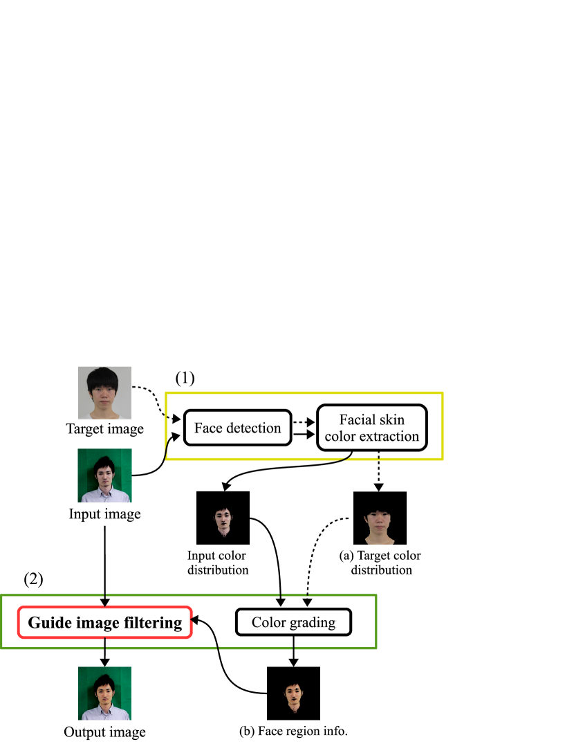
Figure 1: Flow chart of our method.

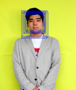
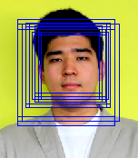
Figure 2: Face detection. (left) Original image, (center) Detected face area (candidates), and (right) Face area in the original image. Blue boxes indicate candidates for the face.

3.1 Face detection

In the first step, we detect an area from head to shoulder (Fig. 2), where we use Haar-cascade detection in OpenCV, also known as the Viola-Jones algorithm [29], for the face detection. The face area is described by $n$ rectangle windows, where $n$ is the number of candidates, with a set of barycentric coordinates $(x,y)$ and the sizes of the detected candidate rectangles $(w,h)$ Fig. 2 (center). The blue boxes in Fig. 2 indicate the detected candidate rectangles. We find the median of $x,y,w,h$ as

$$\begin{array}[]{rlrl}\widehat{x}&:=\text{median}(\{x_{1},\ldots,x_{n}\}),&\widehat{w}&:=\text{median}(\{w_{1},\ldots,w_{n}\}),\\ \widehat{y}&:=\text{median}(\{y_{1},\ldots,y_{n}\}),&\widehat{h}&:=\text{median}(\{h_{1},\ldots,h_{n}\}),\end{array}$$ (1)

where the subscript is the index of the candidate. The rectangle with the median values of the barycentric coordinate $(\widehat{x},\widehat{y})$ is adopted as the final face area. Since the size of the face area $(\widehat{w},\widehat{h})$ depends on the image, the size of the face area is adjusted by:

$$\left(2l\,\widehat{w}+1\right)\times\left(2l\,\widehat{w}+1\right),$$ (2)

where $l$ is the prescribed scale factor.

3.2 Skin color extraction

Rough extraction of the skin color region near the face is performed by a common approach using morphological labeling in the image space and clustering in the color space:

1. We classify the color of each pixel by clustering the color distribution of the entire image in the HSV color space, and for each pixel we allocate the label of the cluster that each pixel belongs to.

2. Some regions are generated by concatenating neighboring pixels with the same labels in the image space, and then we extract regions mainly in the detected face area $\Omega_{\text{rect}}$ (Eq. (2)) and assign them to the facial skin region.

Note that, since the skin color in the detected face area (Sec. 3.1) is known, we may obtain satisfactory results by using simpler approaches such as the k-means method [18] with stable seed cluster selection [2] (i.e., k-means++) for clustering color distributions.

In this paper, for simplicity, we apply k-means clustering [2] to the 1-D distribution of the hue values of the entire image, and we perform the above-mentioned procedures (i) and (ii) to detect the face region $\Omega^{\textit{hue}}_{S}$. Then we perform thresholding on the region $\Omega^{\textit{hue}}_{S}$ for the saturation and value components of every pixel. We define the skin color region $\Omega_{S}$ and the condition for the skin color at pixel $p$ experimentally as follows:

$$\Omega_{S}:=\left\{p\mid p\!\in\!\Omega_{S}^{hue},\ s_{p}\!\in\![\widehat{s}\!-\!0.2,\widehat{s}\!+\!0.2],\ v_{p}\!\in\![0.15,0.95]\right\}$$ (3)

where $\widehat{s}$ is the median of the saturation in the face area. The saturation and the value are normalized to $[0,1]$ and the threshold values are set to excellently extract the facial skin color region on our dataset, which is available on the project page. The number of clusters depends on the photographic environment. We set $k=4$ in this paper.

For our guide image filtering, we define $\Omega_{B}$ and $\Omega_{\partial S}$ using the dilation function, which is a type of morphological operation. They are given as

$$\Omega_{S}^{\prime} :=\text{dilation}(\Omega_{S}),$$ (4)

$$\Omega_{B} :=\overline{\Omega^{\prime}}_{S},$$

$$\Omega_{\partial S} :=\Omega^{\prime}_{S}\setminus\Omega_{S},$$

where $\text{dilation}(\cdot)$ is the dilation function with a structuring element, which consists of a circle with a 20 pixel radius. The overline $\overline{\cdot}$ is the complement and the operator $\setminus$ is the set difference. An example of each region can be seen in Fig. 3.

(a)	(b)	(c)	(d)

Figure 3: Region example. (a) Input image, (b) Skin color region $\Omega_{S}$, (c) Dilated skin color region $\Omega_{S}^{\prime}$, and (d) Each region in the whole image. Pink, red, yellow, and orange indicate each region $\Omega_{S}$, $\Omega_{S}^{\prime}$, $\Omega_{B}$, and $\Omega_{\partial S}$, respectively.

3.3 Color grading by [23]

Color grading (Fig. 4) is performed so as to bring the skin color of the extracted region $\Omega_{S}$ (more specifically the shape of the color distribution) close to the target facial skin color in Fig. 4(a). Color grading transforms the shapes of color distributions (r,g,b 3D coordinates). One may use simpler techniques such as the estimation of a tone curve to modify each RGB component. However, most of the methods need correspondence between the two images, which is not suitable in our case where one transfers the color between the faces of different persons. In our method we use Pitié et al.’s method [23], in which pixel correspondences are not necessary. This method considers the width of the color distribution along a particular axis, iteratively changes it so as to match the specified axis, and then realizes nonlinear reshaping of the color distribution. Since the method yields some artifacts such as blurring artifacts around the edges, we need to address this problem, which is described hereafter.

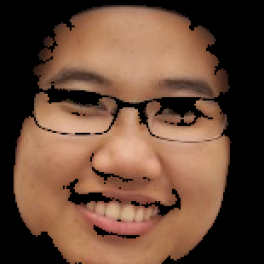
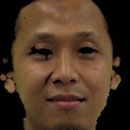
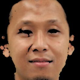
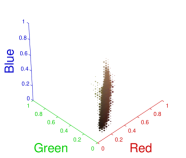
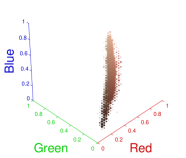
(a) Target (b) Input (c) Corrected

Figure 4: Each extracted facial skin color region and their distributions. The top row shows (left) target color image, (center) input image, and (right) color graded image. The bottom row shows their color distributions in the RGB color space.

3.4 Guide image filtering via optimization

This section expresses our GIF, which uses a guide image to correct the input image, as an optimization based method. Our energy function actually resembles in part that of the image matting method [17] because we focus on and use its data fidelity term (in [17] that is also known as the local linear model), but the design objective is different. Additionally, a similar method has been proposed in high dynamic range imaging [25].

Our guide image filtering reconstructs an image $\mathbf{x}\in\mathbb{R}^{3N}$ where the facial skin color region has a corrected color by using the input image $\mathbf{y}\in\mathbb{R}^{3N}$ and the color grading result, where $N$ is a number of pixels. In the RGB color space ($\mathbb{R}^{3}$), let the pixel value at pixel $j$ of the color corrected image to be solved be $\mathbf{x}_{j}$, the input image be $\mathbf{y}_{j}$, and the guide image be $\mathbf{g}_{j}$ which are given by the color grading in Sec. 3.3. Figure 5 shows each image. Using them, we formulate our guide image filtering as the following convex optimization problem

$$\min_{\mathbf{x,A,b}}\ \underbrace{\sum_{i}\left(\sum_{j\in w_{i}}\|\mathbf{x}_{j}-\mathbf{A}_{i}\mathbf{y}_{j}-\mathbf{b}_{i}\|^{2}_{2}+\varepsilon\|\mathbf{A}_{i}\|^{2}_{F}\right)}_{\text{data fidelity}}$$ (5)

$$\ +\ \underbrace{\iota_{\mathcal{C}_{S}}(\mathbf{x})+\ \iota_{\mathcal{C}_{B}}(\mathbf{x})}_{\text{constraints}},$$

where $\mathbf{A}_{i}\in\mathbb{R}^{3\times 3}$ and $\mathbf{b}_{i}\in\mathbb{R}^{3}$ are a scaling matrix and an offsetting vector to approximate $\mathbf{y}_{j}$ to $\mathbf{x}_{j}$ for each pixel $i$, $w_{i}$ is a square window around pixel $i$, and $\mathcal{C}_{S}$ and $\mathcal{C}_{B}$ are given by

$$\mathcal{C}_{S} :=\textstyle\left\{\mathbf{x}\mid\sqrt{\sum_{p\in\Omega_{S}}\|\mathbf{x}_{p}-\mathbf{g}_{p}\|^{2}}\leq\eta_{S}\right\},$$ (6)

$$\mathcal{C}_{B} :=\textstyle\left\{\mathbf{x}\mid\sqrt{\sum_{q\in\Omega_{B}}\|\mathbf{x}_{q}-\mathbf{y}_{q}\|^{2}}\leq\eta_{B}\right\}.$$

Terms in the top row correspond to [17], where $\|\cdot\|_{2}$ and $\|\cdot\|_{F}$ denote the $\ell_{2}$ norm and Frobenius norm respectively, and we use them as a data fidelity that reflects textures and local contrasts of $\mathbf{y}$ onto $\mathbf{x}$. The second and third terms are constraints expressed by the following indicator function:

$$\iota_{\mathcal{C}}(\mathbf{x}):=\left\{\begin{array}[]{ll}0&\text{if}\ \mathbf{x}\in{\mathcal{C}},\\ +\infty&\text{otherwise}.\end{array}\right.$$ (7)

The second term brings the facial skin color close to that of the guide image $\mathbf{g}$ in the facial skin color region $\Omega_{S}$. The third term keeps the color of the background the same as the original image $\mathbf{y}$ in $\Omega_{B}$. For reducing undesirable artifacts arising from the guide image, we add a constraint that the color difference at each pixel does not exceed $\eta$.

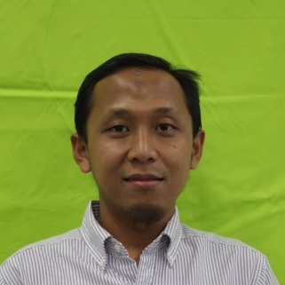
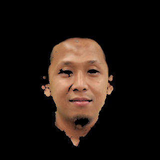
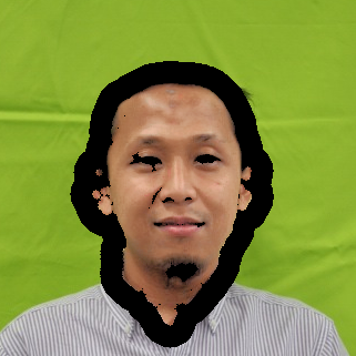
$\mathbf{y}$	$\mathbf{g}_{p},\ \forall p\in\Omega_{S}$	$\mathbf{g}_{p},\ \forall p\in\Omega_{S}$ $\mathbf{y}_{q},\ \forall q\in\Omega_{B}$	$\mathbf{x}$

Figure 5: Guide image filtering. From left: Input image, Guide image, Target color in $\Omega_{B}$ and $\Omega_{S}$, and Color transformed image.

Note that we purposefully represent the second and third terms as constraint formulation over unconstrained one, e.g., the second term can be replaced with a regularizer $\lambda\sqrt{\sum_{p\in\Omega_{S}}\|\mathbf{x}_{p}-\mathbf{g}_{p}\|^{2}}$ where $\lambda$ is a balancing parameter. This is because $\eta$ can be controlled more intuitively than $\lambda$, and it allows us to adaptively change $\eta$ depending on the area of $\Omega_{s}$ (see the next Sec. 4). Such advantages of the formulation have been addressed in the literature of image restoration based on convex optimization [7, 9, 1, 28, 19, 6, 20].

Among convex optimization algorithms, we adopt a monotone version of the fast iterative shrinkage-thresholding algorithm (MFISTA) [5] to solve (5) because it is a first-order method that achieves a sublinear global rate of convergence, namely, computationally efficient and very fast. The algorithm solves an optimization problem of the form:

$$\underset{\mathbf{x}}{\min}\ f(\mathbf{x})+h(\mathbf{x}),$$ (8)

where $f(\mathbf{x})$ is a differentiable convex function with a Lipschitz continuous gradient and $h(\mathbf{x})$ is a proper lower semicontinuous convex function. The problem (8) is calculated by the proximity operator . For given $\mathbf{x}^{0}=:\mathbf{v}^{1}\in\mathbb{R}^{N}$ and $t^{1}:=1$, the iteration of the MFISTA consists of the following five steps:

$$\left\lfloor\begin{aligned} \hat{\mathbf{z}}^{k}&=\displaystyle\mathbf{v}^{k}-\frac{1}{L}\nabla f(\mathbf{v}^{k}),\\ \mathbf{z}^{k}&=\displaystyle\text{prox}_{h/L}\left(\hat{\mathbf{z}}^{k}\right),\\ \mathbf{x}^{k}&=\displaystyle\arg\min\{\ f(\mathbf{z})+h(\mathbf{z})\ |\ \mathbf{z}\in\{\mathbf{z}^{k},\mathbf{x}^{k-1}\}\},\\ t^{k+1}&=\displaystyle\frac{1+\sqrt{1+4(t^{k})^{2}}}{2},\\ \mathbf{v}^{k+1}&=\displaystyle\mathbf{x}^{k}+\frac{t^{k}}{t^{k+1}}(\mathbf{z}^{k}-\mathbf{x}^{k})+\frac{t^{k}-1}{t^{k+1}}(\mathbf{x}^{k}-\mathbf{x}^{k-1}),\end{aligned}\right.$$ (9)

where “prox” is the proximity operator and $1/L$ is the step size.

In order to apply the MFISTA to our problem (5), we set

$$f(\mathbf{x}) :=\sum_{i}\left(\sum_{j\in w_{i}}\|\mathbf{x}_{j}-\mathbf{A}_{i}\mathbf{y}_{j}-\mathbf{b}_{i}\|^{2}_{2}+\varepsilon\|\mathbf{A}_{i}\|^{2}_{F}\right),$$ (10)

$$h(\mathbf{x}) :=\iota_{\mathcal{C}_{S}}(\mathbf{x})+\ \iota_{\mathcal{C}_{B}}(\mathbf{x}).$$

To compute the gradient $\nabla f(\mathbf{x})$, we use a method similar to [13], which is an accelerated version of [17]. We compute each value of $[\nabla f(\mathbf{x})]_{i}\in\mathbb{R}^{3}$ as follows:

$$\mathbf{A}^{\ast}_{i} =\Delta_{i}^{-1}\left(\frac{1}{|w_{i}|}\left(\displaystyle\sum_{j\in w_{i}}\mathbf{y}_{j}\mathbf{x}_{j}^{\top}\right)-\overline{\mathbf{y}}_{i}\overline{\mathbf{x}}_{i}^{\top}\right),$$ (11)

$$\mathbf{b}^{\ast}_{i} =\overline{\mathbf{x}}_{i}-\mathbf{A}_{i}^{\ast}\overline{\mathbf{y}}_{i},$$ (12)

$$[\nabla f(\mathbf{x})]_{i} =|w_{i}|\mathbf{y}_{i}-\left(\left(\sum_{j\in w_{i}}\mathbf{A}_{j}^{\ast}\right)\mathbf{y}_{i}+\left(\sum_{j\in w_{i}}\mathbf{b}_{j}^{\ast}\right)\right),$$ (13)

where $\overline{\mathbf{x}}_{i}=[\overline{x}^{R}_{i}\ \overline{x}^{G}_{i}\ \overline{x}^{B}_{i}]^{\top}$ and $\overline{\mathbf{y}}_{i}=[\overline{y}^{R}_{i}\ \overline{y}^{G}_{i}\ \overline{y}^{B}_{i}]^{\top}$ are mean value vectors of each color in a square window $w_{i}$, $|w_{i}|$ is the number of pixels in $w_{i}$, $\Delta=\boldsymbol{\Sigma}_{i}+\frac{\varepsilon}{|w_{i}|}\mathbf{U}\in\mathbb{R}^{3\times 3}$, $\boldsymbol{\Sigma}_{i}=\frac{1}{|w_{i}|}\left(\sum_{j\in w_{i}}\mathbf{y}_{j}\mathbf{y}_{j}^{\top}\right)-\overline{\mathbf{y}}_{i}\overline{\mathbf{y}}_{i}^{\top}$ is a covariance matrix, and $\mathbf{U}$ is an identity matrix.

The proximity operator $\text{prox}_{h/L}$ in (9) consists of two functions which are the second and third terms of (5) which handle different regions, $\Omega_{S}$ and $\Omega_{B}$, respectively that satisfies, i.e., $\Omega_{S}\cap\Omega_{B}=\{0\}$. Therefore, $\text{prox}_{h/L}$ can be calculated using

$$\mathbf{z}_{i}:=[\text{prox}_{h/L}(\hat{\mathbf{z}})]_{i}=$$ (14)

$$\begin{cases}\ \displaystyle\hat{\mathbf{z}}_{i}+\eta_{S}\frac{\hat{\mathbf{z}}_{i}-\mathbf{g}_{i}}{\sqrt{\sum_{p\in\Omega_{S}}\|\hat{\mathbf{z}}_{p}-\mathbf{g}_{p}\|^{2}}}&\text{if}\ \hat{\mathbf{z}}\notin\mathcal{C}_{S}\land\ i\in\Omega_{S},\\ \ \displaystyle\hat{\mathbf{z}}_{i}+\eta_{B}\frac{\hat{\mathbf{z}}_{i}-\mathbf{y}_{i}}{\sqrt{\sum_{q\in\Omega_{B}}\|\hat{\mathbf{z}}_{q}-\mathbf{y}_{q}\|^{2}}}&\text{if}\ \hat{\mathbf{z}}\notin\mathcal{C}_{B}\land\ i\in\Omega_{B},\\ \ \hat{\mathbf{z}}_{i}&\text{otherwise}.\end{cases}$$

This process corresponds to a $\ell_{2}$-ball projection with a region constraint.

Finally, we update $\mathbf{x,z,v},t$ using the procedure in (9), then the solution $\mathbf{x}$ becomes our GIF result.

4 Results and discussion

In this section, we show the results obtained through the proposed process . The range of RGB values is normalized to be in the range $[0,1]$. The prescribed scale factor $l$ in Sec. 3.1 is set to $2.0$. The filter window sizes used in Sec. 3.4 and Sec. Appendix A: Fore/Background segmentation by matting are $19\times 19$ and $31\times 31$, respectively. $\eta_{S}=5|\Omega_{S}|\times 10^{-4}$ and $\eta_{B}=5|\Omega_{B}|\times 10^{-10}$ are used, where $|\Omega_{(\cdot)}|$ indicates the number of pixels contained in the region $\Omega_{(\cdot)}$. $L$ in MFISTA is set to 500.

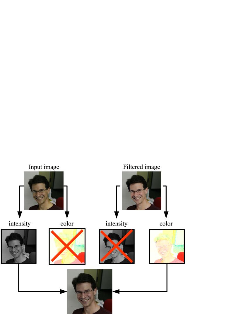
Figure 6: Simple luminance correction. Input image and filtered image are decomposed into intensity components and color components, respectively by (15), then the intensity component of the input image and the color component of the filtered image are combined by (16).

(a) Target

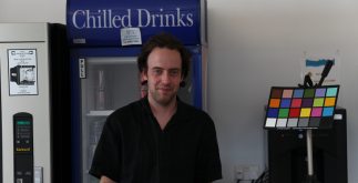
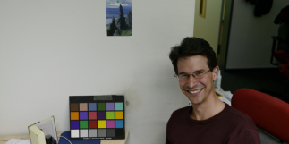
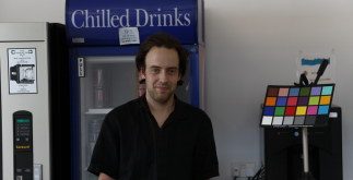
(b) Input (c) Output

Figure 7: Our facial skin color correction. (a) Target facial skin color image, (b) Input image, and (c) Output image using our facial skin color correction. The target image is in Shin et al.’s dataset [26] and the input images are in the Gehler dataset [10].

(a) Target

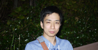
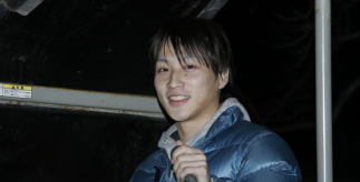
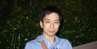
(b) Input (c) Output

Figure 8: Our facial skin color correction on the flash images. (a) Target facial skin color image, (b) Input flash images, (c) Output images using our facial skin color correction.

Our filtering often flattens the gradation of the input images caused by shadows. It yields unnatural images as shown in the top of Fig. 6, where the input image is input to our algorithm and the filtered image is a result of our guide image filtering. For the luminance correction, each pixel color value of the image is decomposed into a color component $\mathbf{x}_{i}^{C}\in\mathbb{R}^{3}$ and an intensity component $x_{i}^{I}\in\mathbb{R}^{1}$ as follows

$$x_{i}^{I} =\frac{x_{i}^{R}}{\|\mathbf{x}_{i}\|_{1}}x_{i}^{R}+\frac{x_{i}^{G}}{\|\mathbf{x}_{i}\|_{1}}x_{i}^{G}+\frac{x_{i}^{B}}{\|\mathbf{x}_{i}\|_{1}}x_{i}^{B},$$ (15)

$$\mathbf{x}_{i}^{C} =\frac{\mathbf{x}_{i}}{x_{i}^{I}},$$

where the superscripts $R$,$G$, and $B$ indicate each color component. This decomposition procedure is same as [8].

The input image and the filtered image are decomposed into the two components by (15), and then the intensity component of the input image $y_{i}^{I}$ and the color component of the filtered image $\mathbf{x}_{i}^{C}$ are combined as follows

$${\mathbf{x}_{i}}^{\prime}=y_{i}^{I}\mathbf{x}_{i}^{C}.$$ (16)

Figure 6 shows this procedure and its effectiveness.

Figure 8 (hereafter indexes are swapped due to figure positions) shows the result of our skin color correction. The area around the face in the input image has color distortion due to the lighting conditions and background color. Our result has a white balanced facial skin color similar to the target facial skin color. Sometimes when we take a photograph in dark surroundings, the results sometimes have unnatural face colors (Fig. 8(b)) due to the camera flash. Hence, we apply our proposed method to flash images in dark surroundings to reduce undesirable effects of artificial lights. Figure 8(c) shows the flash image editing results using our method. One can see that unnatural colors of the original image are corrected to natural colors by our method.

4.1 Automatic yearbook style photo generation

This section presents automatic yearbook style photo generation using our guided facial skin correction method and pre/post-processing procedure. It takes a long time to manually process a large number of images. Our algorithm generates a yearbook style photo in a short amount of time.

We first crop a photo with our face detection procedure as a pre-processing procedure (the red box in Fig. 9), and then correct the facial skin color. Finally, the noisy background is replaced to clear the background as a post-processing procedure (the blue boxes in Fig. 9).

4.1.1 Face area cropping

In Sec. 3.1, we detect the face area of a photo. Then we unify the sizes of the cropped images by expansion and reduction. The crop size is roughly adjusted according to the image size. The image size after cropping and resizing is $320\times 320$ ($h\times w$) in this experiment.

4.1.2 Background replacement by alpha blending

We separate the image information of the foreground and background regions and assign a value $\alpha_{i}:=[0,1]$ to them. Using the values as labels, the relationship between the foreground $\mathbf{f}_{i}$, background $\mathbf{b}_{i}$ (different from that in (5)), and original image $\mathbf{y}_{i}$ at each pixel is given as follows:

$$\mathbf{y}_{i}:=\mathbf{f}_{i}+\mathbf{b}_{i},\quad\mathbf{f}_{i}:=(1-\alpha_{i})\mathbf{y}_{i},\quad\mathbf{b}_{i}:=\alpha_{i}\mathbf{y}_{i}.$$ (17)

The label $\alpha$ at each pixel is the blending rate, and called alpha-mat. Replacement of the background with another background $\mathbf{z}$ is performed by

$$\mathbf{y}^{\prime}_{i}:=\mathbf{f}_{i}+\alpha_{i}\mathbf{z}_{i}.$$ (18)

An estimation of the alpha-mats is described in Appendix A.

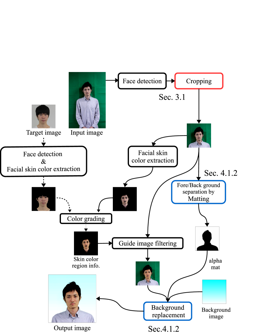
Figure 9: Flow chart of auto yearbook style photo generation. The red box indicates a pre-processing procedure and the blue boxes indicate a post-processing procedure.

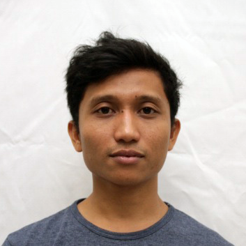
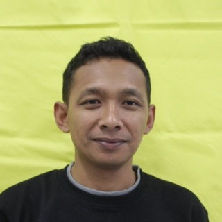
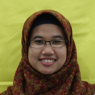
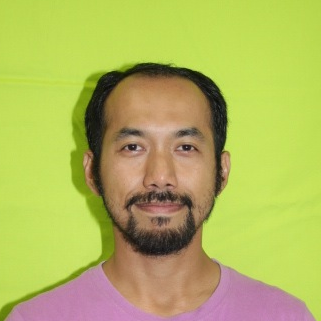
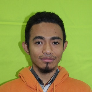
(a) Target	(b) Original images
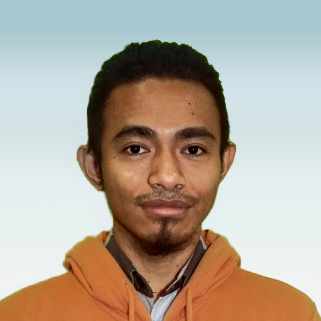
	(c) Yearbook style images

Figure 10: Results of automatic yearbook style photo generation using our method. (a) Target facial skin color image, (b) Original images which have a background color similar to the facial skin color, (c) Yearbook style images using our algorithm.

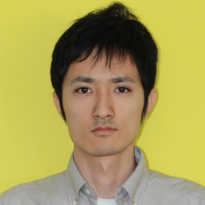
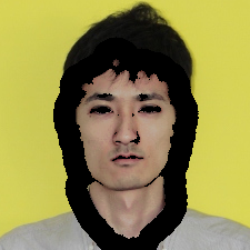
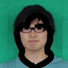
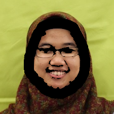
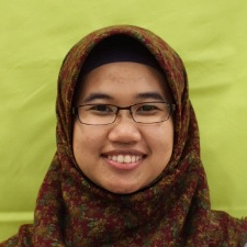
(a) Original	(b) Guide	(c) Colorization [16]	(d) JBU [15]	(e) Ours

Figure 11: Supplement quality comparison with similar methods. (a) Original, (b) Guide, (c) Colorization for each RGB layer [16], (d) Joint Bilaterl Upsampling (JBU) for each RGB layer [15], and (e) Our guided filtering (5). The black pixels in (b) represents a hole region and each red arrow indicates an artifact.

Figure 10 shows the results of our automatic yearbook style photo generation. Our algorithm generates the yearbook style photos from the original images using the target image.

We implement the whole algorithm in MATLAB and OpenCV (C++), respectively, and the total execution time is within 11 sec. on a 3.20 GHz Core i5 CPU, i.e., face detection (Sec. 3.1) is 5 sec., facial color extraction (Sec. 3.2) is 1 sec., color grading (Sec. 3.3) is 2 sec., GIF (Sec. 3.4) is 2 sec., and matting (Sec. 4.1.2) is 1 sec., respectively.

4.2 Comparison with various conventional method

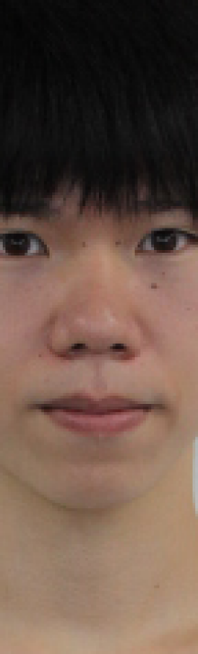
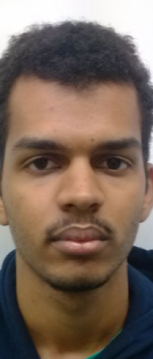
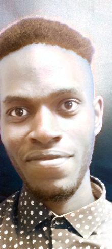
(a) Target	(b) Original	(c) [24] with [23]	(d) [11]	(e) [21]	(f) Ours

Figure 12: Comparison with the existing methods. (a) Target, (b) Original, (c) [24] with [23], (d) NRDC [11], (e) Jaesik et al. [21], and (f) Our method.

(a) Target	(b) Original	(c) Background replacement
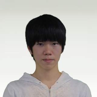
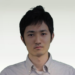
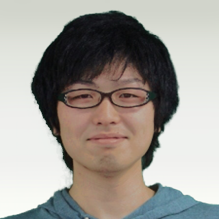
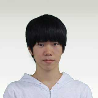
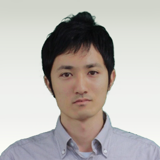
	(d) [26]	(e) Ours

Figure 13: Comparison with the background replacement result and [26]. (a) Target facial skin color image, (b) Original images, (c) The background replacement result as a example, (d) The style transfer result by [26], and (e) The yearbook style photo using our algorithm.

Figure 11 compares our method with supplement methods [16, 15]. For the methods, we process each RGB color layer because they are proposed for color components in YUV color space. Since colorization [16] just spreads colors to boundaries, the result does not have the details of the original image. Joint Bilateral Upsampling [15] computes pixel values in hole regions by joint-filtering. We can see a contrast reduction in the top and the middle rows in Fig. 11. The blue arrows and the red arrows indicate artifacts of each method. Meanwhile our guide image filtering outputs sharp details of the original image while keeping the guide image color.

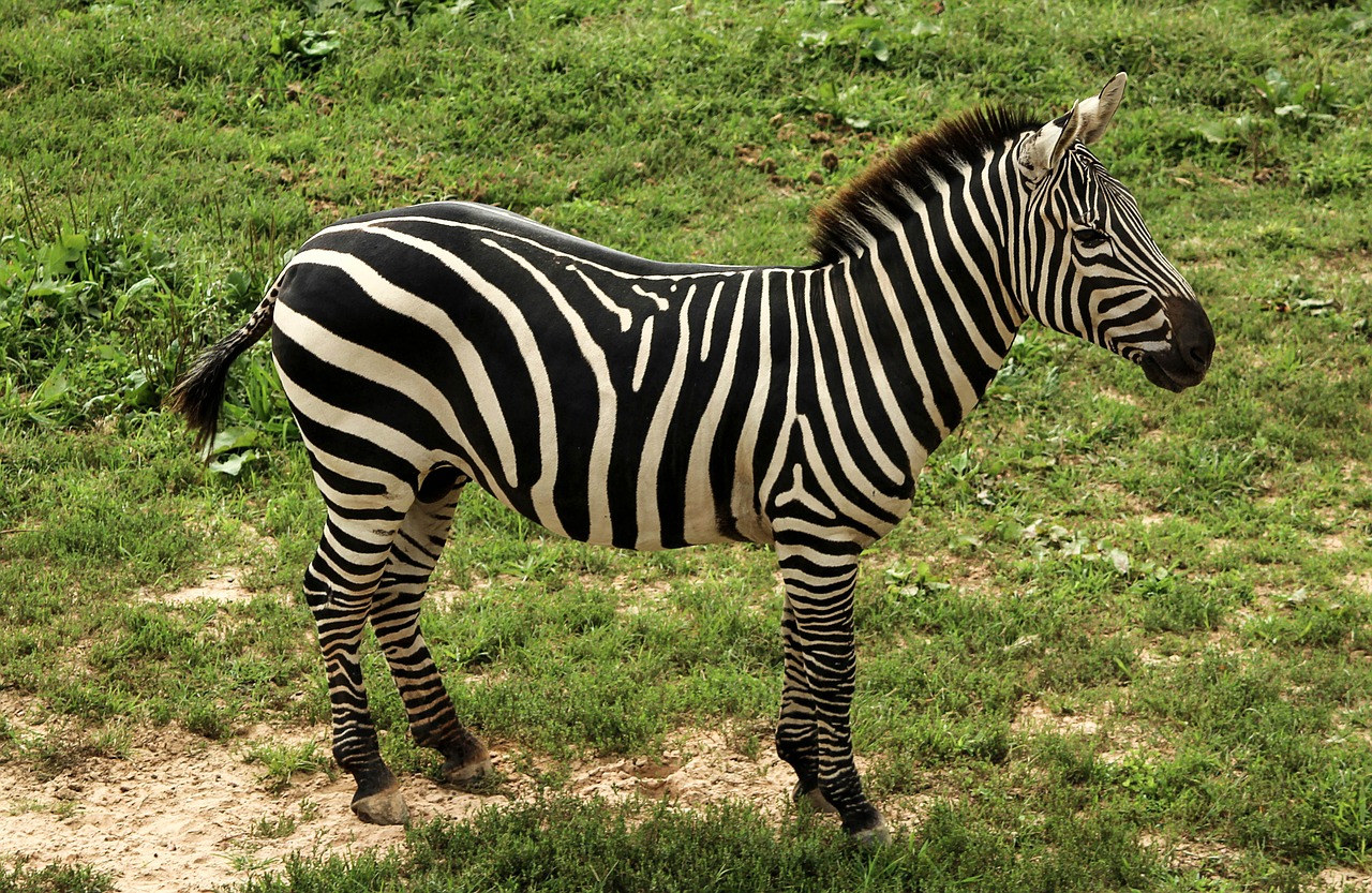
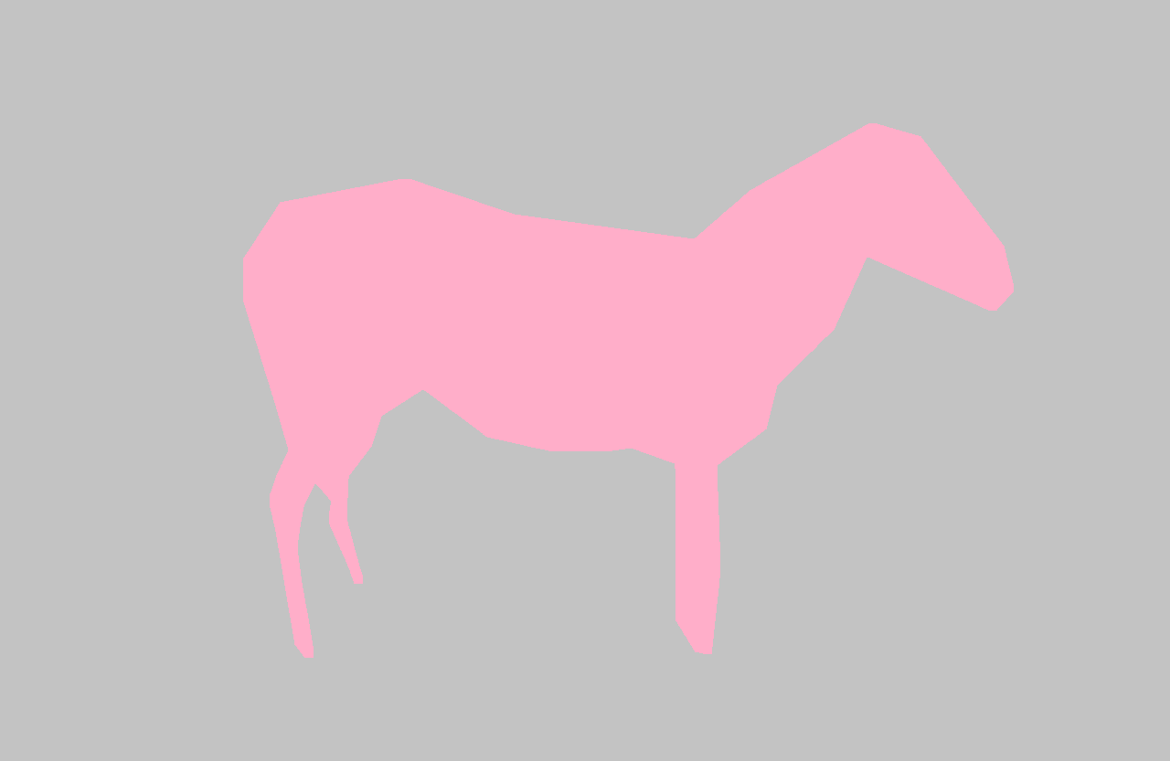
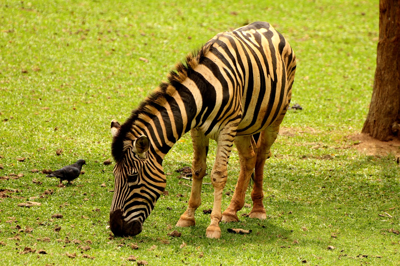
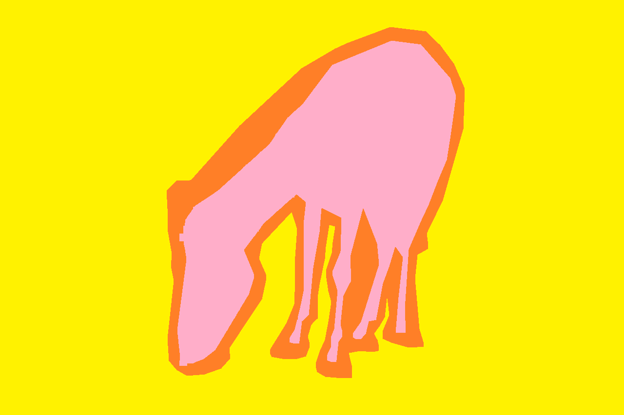
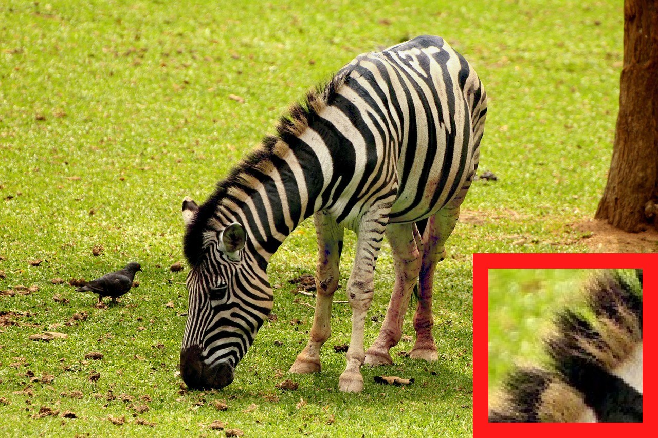
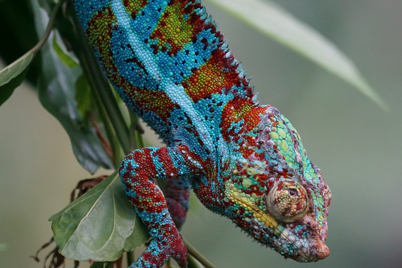
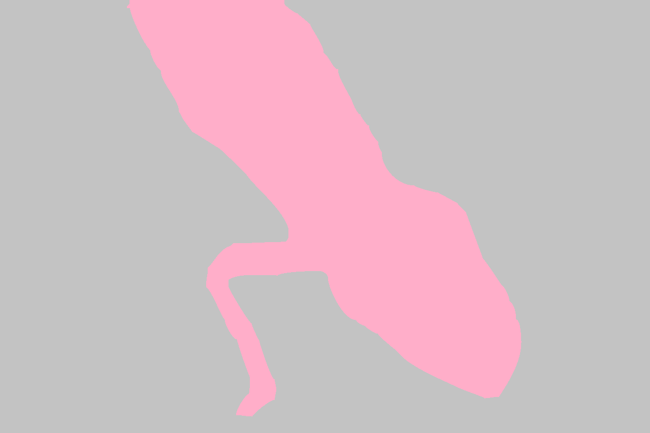
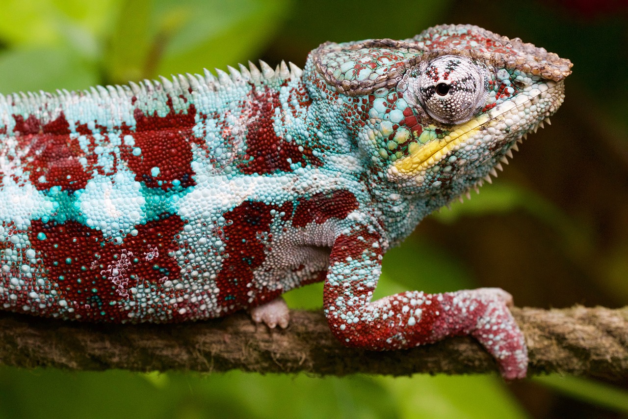
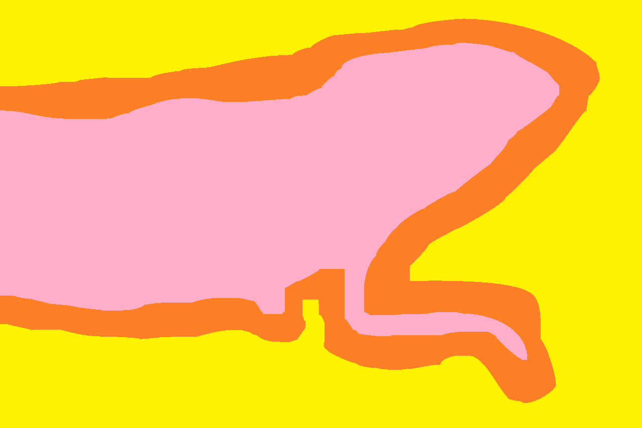
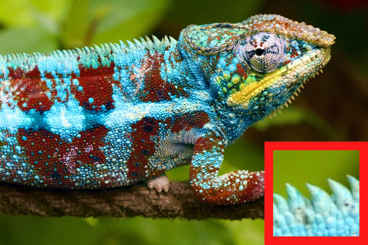
(a) Target	(b) Each region	(c) Source	(d) Each region	(e) Result

Figure 14: Semi-automatic color correction. (a) Target, (b) Each region in target image, (c) Source, (d) Each region in source image, and (e) Result. Colors in (b) and (d) indicate each region as Fig. 3. The source and target images are available at https://pixabay.com.

Figure 12 shows a comparison with existing color transfer methods. For the results (c), Pitié et al.’s method [23] transforms the color distribution of the input image to the target image one, then gain noise artifacts of the color transformed input image are removed by Rabin et al.’s method [24]. The gain noise artifacts can be seen in [23]. In the results of the color grading [24] with[23], the face and the background of the resultant image hava a similar color since this method is a uniform color transfer method. In addition, this method takes a long time because it needs iterative bilateral filtering. In the non-rigid dense correspondence (NRDC) method [11] and Jaesik et al. [21], the improvement in facial color is small, and the regions around the clothes are discolored. However, in our method (e), color correction is successfully done over the entire face, and look more natural. From the above results, the proposed process gives satisfactory results despite the automatic processing.

Figure 13 shows a comparison with a background replacement result of the original image and [26]. The background replacement result has a distorted facial skin color due to the background color. Shin et al.’s method transfers a style from an input image to a target image. Although the facial skin color of the result is almost the same as the target image one, this method cannot correct skin color of a person wearing glasses to the skin color of the target image. Our algorithm generates an image which has the target facial skin color even if a person wears glasses.

4.3 Semi-automatic color correction

Our method can correct other images, such as animal photographs. Our color correction method requires some regions, which are $\Omega_{S}$ as a foreground and $\Omega_{B}$ as a background. Many methods have been proposed to detect face regions, but accurate object detection in natural scenes is still a challenging problem.

For color correction in natural scenes such as Fig. 14(c), we make each region manually as (b) and (d), where the colors indicate the region corresponding to Fig. 3, respectively. Finally, our method adjusts the object color of the source image to the target one automatically. Figure14(e) shows natural scene color correction results and the red box shows that our method corrects the colors of main object without boundary artifacts. By implementating an automatic object detection method, this application will be an auto-application.

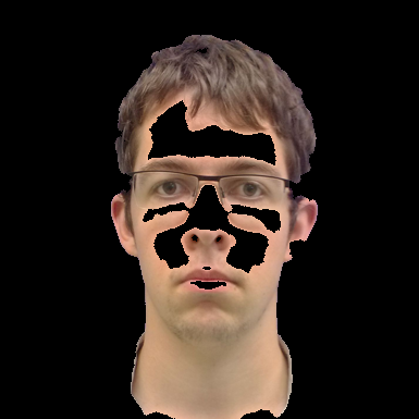
(a) Original images	(b) Extracted skin	(c) Result

Figure 15: Bad results of our method due to the skin color extraction phase. In the original image the face and hair are a similar color.

4.4 Limitation

Figure 15 shows example images where our method does not work well. The face and hair are a similar color, hence, the facial skin color extraction process gets regions other than the face region (Fig. 15(b)). As a result, our method outputs an image with a similar color between the face and hair (Fig. 15(c)). Actually, the facial skin color extraction process seldom gets other regions even if the subject does not have white skin, so the guide image filtering results in the same color between the face and the other extracted regions.

5 Conclusions

This paper presents a guided facial skin color correction method. The color grading method used in the procedure can be thought of as a correction method using a target (guide) image in a color space. On the other hand, our GIF can be thought of as a correction method using a guide image in an image space. In future work, we will consider combining both methods to extend the range of constraint expressions to color correction so as to obtain more natural results.

Appendix A: Fore/Background segmentation by matting

To obtain the alpha-mats that give natural blending results, we employ a closed form matting method [13] because the algorithm is also used in Sec. 3.4 and can be diverted. The method is based on continuous optimization in which labels are obtained as real numbers (soft labels) in the range of $[0,1]$. However this method requires semantics (user assisted information) for fore/background regions around their boundaries. In order to avoid user assistance, we also employ a region growing method used in an earlier matting method [27] and perform matting iteratively. The details are shown in Fig. 16 and described as follows:

1. As the initial foreground $\Omega_{F}$, in addition to the skin color region $\Omega_{S}$, the hair region above the face (a black large region is roughly selected), and the clothes region below the face are used. As the initial background $\Omega_{B}$, two rectangular regions on the left and right sides of the face are used.

2. Matting [13] with the preconditioning conjugate gradient method is performed. A soft label $\alpha_{i}\in[0,1]$ is obtained at each pixel.

3. The pixels that are strongly regarded as foreground or background are added to the initial region, which is generated in (a), for the next iteration:
   $\Omega^{+}_{B}:=\{i\ |\ \alpha_{i}\leq 0.2\}$, $\Omega^{+}_{F}:=\{i\ |\ 0.8\leq\alpha_{i}\}$ and then
   $\{\alpha_{i}:=0\ |\ i\in\Omega_{B}\cup\Omega^{+}_{B}\}$, $\{\alpha_{i}:=1\ |\ i\in\Omega_{F}\cup\Omega^{+}_{F}$}.

4. Steps (b) and (c) are repeated a few times (4 times, in our experiment). The radius of the window size is halved to implement a coarse-to-fine approach.

5. To reduce neutral colors and enhance them to be close to 0 or 1, a sigmoid function is applied to the alpha-mat:
   $\alpha_{i}:=(1+\exp(-10(\alpha_{i}-0.5)))^{-1}$.

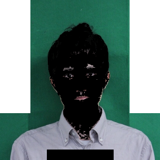
(a)	(b)	(c)	(d)	(e)

Figure 16: Image matting with region growing.

References

- [1] M. V. Afonso, J. M. Bioucas-Dias, and M. A. T. Figueiredo. An augmented Lagrangian approach to the constrained optimization formulation of imaging inverse problems. IEEE Trans. Image Process. (TIP), 20(3):681–695, Mar. 2011.
- [2] David Arthur and Sergei Vassilvitskii. K-means++: The advantages of careful seeding. In Proc. Annual ACM-SIAM Symp. Discrete Algorithms, pages 1027–1035. Society for Industrial and Applied Mathematics, 2007.
- [3] Tatsuya Baba, Paul Perrotin, Yusuke Tatesumi, Keiichiro Shirai, and Masahiro Okuda. An automatic yearbook style photo generation method using color grading and guide image filtering based facial skin color. In Proc. IAPR Asian Conf. Pattern Recognit. (ACPR), pages 1–6, 2015.
- [4] Narze Batool and Rama Chellappa. Detection and inpainting of facial wrinkles using texture orientation fields and Markov random field modeling. IEEE Trans. Image Process. (TIP), 23(9):3773–3788, 2014.
- [5] Amir Beck and Marc Teboulle. Fast gradient-based algorithms for constrained total variation image denoising and deblurring problems. IEEE Trans. Image Process. (TIP), 18(11):2419–2434, 2009.
- [6] G. Chierchia, N. Pustelnik, J.-C. Pesquet, and B. Pesquet-Popescu. Epigraphical projection and proximal tools for solving constrained convex optimization problems. Signal, Image Video Process., 9(8):1737–1749, Nov. 2015.
- [7] P. L. Combettes and J. C. Pesquet. Image restoration subject to a total variation constraint. IEEE Trans. Image Process. (TIP), 13(9):1213–1222, Sept. 2004.
- [8] Elmar Eisemann and Frédo Durand. Flash photography enhancement via intrinsic relighting. ACM Trans. Graph. (TOG), 23(3):673–678, 2004.
- [9] J. M. Fadili and G. Peyré. Total variation projection with first order schemes. IEEE Trans. Image Process. (TIP), 20(3):657–669, Mar. 2011.
- [10] Peter Vincent Gehler, Carsten Rother, Andrew Blake, Tom Minka, and Toby Sharp. Bayesian color constancy revisited. In Proc. IEEE Conf. Comput. Vis. Pattern Recognit. (CVPR), pages 1–8, 2008.
- [11] Yoav HaCohen, Eli Shechtman, Dan B Goldman, and Dani Lischinski. Non-rigid dense correspondence with applications for image enhancement. ACM Trans. Graph. (TOG), 30(4):70:1–70:10, 2011.
- [12] Yoav HaCohen, Eli Shechtman, Dan B. Goldman, and Dani Lischinski. Optimizing color consistency in photo collections. ACM Trans. Graph. (TOG), 32(4):38:1–38:10, 2013.
- [13] Kaiming He, Jian Sun, and Xiaoou Tang. Fast matting using large kernel matting Laplacian matrices. In Proc. IEEE Conf. Comput. Vis. Pattern Recognit. (CVPR), pages 2165–2172, 2010.
- [14] Kaiming He, Jian Sun, and Xiaoou Tang. Guided image filtering. IEEE Trans. Pattern Anal. Mach. Intelli. (TPAMI), 35(6):1397–1409, 2013.
- [15] Johannes Kopf, Michael F. Cohen, Dani Lischinski, and Matt Uyttendaele. Joint bilateral upsampling. ACM Trans. Graph. (TOG), 26(3):96:1–96:5, 2007.
- [16] Anat Levin, Dani Lischinski, and Yair Weiss. Colorization using optimization. ACM Trans. Graph. (TOG), 23(3):689–694, 2004.
- [17] Anat Levin, Dani Lischinski, and Yair Weiss. A closed-form solution to natural image matting. IEEE Trans. Pattern Anal. Mach. Intelli. (TPAMI), 30(2):228–242, 2008.
- [18] Stuart P. Lloyd. Least squares quantization in PCM. IEEE Trans. Info. Theory, 28(2):129–137, 1982.
- [19] Shunsuke Ono and Isao Yamada. Second-order total generalized variation constraint. In Proc. IEEE Int. Conf. Acoust., Speech, Signal Process. (ICASSP), pages 4938–4942, May 2014.
- [20] Shunsuke Ono and Isao Yamada. Signal recovery with certain involved convex data-fidelity constraints. IEEE Trans. Signal Process., 63(22):6149–6163, Nov. 2015.
- [21] Jaesik Park, Yu-Wing Tai, Sudipta Sinha, and In So Kweon. Efficient and robust color consistency for community photo collections. In Proc. IEEE Conf. Comput. Vis. Pattern Recognit. (CVPR), pages 430–438, 2016.
- [22] Georg Petschnigg, Richard Szeliski, Maneesh Agrawala, Michael Cohen, Hugues Hoppe, and Kentaro Toyama. Digital photography with flash and no-flash image pairs. ACM Trans. Graph. (TOG), 23(3):664–672, 2004.
- [23] François Pitié, Anil C. Kokaram, and Rozenn Dahyot. Automated colour grading using colour distribution transfer. Comput. Vis. Image Underst., 107(1–2):123–137, 2007.
- [24] Julien Rabin, Julie Delon, and Yann Gousseau. Regularization of transportation maps for color and contrast transfer. In Proc. IEEE Int. Conf. Image Process. (ICIP), pages 1933–1936, 2010.
- [25] Qi Shan, Jiaya Jia, and Michael S. Brown. Globally optimized linear windowed tone mapping. IEEE Trans. Visuali. Comupt. Graph., 16(4):663–675, 2010.
- [26] YiChang Shih, Sylvain Paris, Connelly Barnes, William T. Freeman, and Frédo Durand. Style transfer for headshot portraits. ACM Trans. Graph. (TOG), 33(4):148:1–148:14, July 2014.
- [27] Jian Sun, Jiaya Jia, Chi-Keung Tang, and Heung-Yeung Shum. Poisson matting. ACM Trans. Graph. (TOG), 23(3):315–321, 2004.
- [28] T. Teuber, G. Steidl, and R. H. Chan. Minimization and parameter estimation for seminorm regularization models with -divergence constraints. Inverse Problems, 29(3), 2013.
- [29] Paul Viola and Michael Jones. Rapid object detection using a boosted cascade of simple features. In Proc. IEEE Conf. Comput. Vis. Pattern Recognit. (CVPR), volume 1, pages I–511–I–518, 2001.