Artificial proto-modelling with simplified-model results from the LHC

Abstract

We present a novel approach to identify potential dispersed signals of new physics in the slew of published LHC results. It employs a random walk algorithm to introduce sets of new particles, dubbed “proto-models”, which are tested against simplified-model results from ATLAS and CMS searches for new physics by exploiting the SModelS software framework. A combinatorial algorithm identifies the set of analyses and/or signal regions that maximally violates the Standard Model hypothesis, while remaining compatible with the entirety of LHC constraints in our database. Crucial to the method is the ability to construct a reliable likelihood in proto-model space; we explain the various approximations which are needed depending on the information available from the experiments, and how they impact the whole procedure.

1 Introduction

Searches for new physics at the LHC are usually pursued on a channel-by-channel basis. A plethora of experimental analyses are thus performed in many different final states, and the outcomes interpreted as limits on new particles in the context of specific Beyond the Standard Model (BSM) scenarios, again for each search channel separately. The disadvantage of this kind of hypothesis testing—which is also done on the theory side by comparing signal predictions of specific BSM incarnations to the experimental limits—is that only a small part of the overall available data is used. Small effects of dispersed signals, which will show up simultaneously in different final states and/or signal regions, might easily be missed, or disregarded as statistical fluctuations.

A more global exploration of the LHC data is in order. As an attempt in this direction, we presented in [1] the prototype of a statistical learning algorithm that identifies potential dispersed signals in the slew of published LHC analyses, building candidate “proto-models ” from them, while remaining compatible with the entirety of LHC results. Such proto-models may then be scrutinised further in dedicated analyses and, in case of a discovery, help to eventually unravel the concrete underlying BSM theory. The ultimate goal is a data-driven bottom-up approach to the quest of new physics with minimal theoretical bias. Being easily extendable, it should eventually also allow one to fold in additional information from other (future) experiments to continuously improve the picture of what data is telling us about BSM physics.

2 The walker algorithm

At present, our statistical learning algorithm is based on the concept of simplified models, exploiting the SModelS [2, 3, 4, 5] software framework and its large database of experimental results. It employs a Markov Chain Monte Carlo (MCMC)-type random walk through proto-model space, adding or removing new particles, and randomly changing their cross sections and branching ratios. This is coupled to a combinatorial algorithm, which identifies the set of analyses and signal regions that maximally violates the Standard Model (SM) hypothesis.

The algorithm to comb through proto-model parameter space in order to identify the models that best fit the data is dubbed the walker. It is composed of several building blocks, or “machines” that interact with each other in a well-defined fashion:

1. Starting with the Standard Model, the builder creates proto-models, randomly adding or removing new particles and changing any of the proto-model parameters.

2. The proto-model is then passed on to the critic, which checks the model against the database of simplified-model results to determine an upper bound on an overall signal strength ($\mu_{\rm max}$).

3. The combiner identifies all possible combinations of results and constructs a combined likelihood for each subset.

An essential aspect in our procedure is that that neither the number nor the kind of the new particles is fixed. Instead, the BSM particle content, the particle masses, production cross sections and decay branching ratios (BRs) are taken as free parameters of the proto-models. This implies a parameter space of varying dimensionality for the MCMC-type random walks!

3 Proto-model construction rules

Proto-models are not intended to be fully consistent theoretical models; therefore their properties are not bound by higher-level theoretical assumptions on the underlying BSM theory. Nonetheless, for practical purposes, we have to make a number of assumptions.

Concretely, in this work we assume that all particles either decay promptly or are fully stable at detector scales. Moreover, since we make extensive use of simplified-model results from searches for supersymmetry (SUSY), we impose that all BSM particles are odd under a $\mathcal{Z}_{2}$-type symmetry, so they are always pair produced and always cascade decay to the lightest state. The Lightest BSM Particle (LBP) is taken to be stable and electrically and color neutral, and hence is a dark matter candidate. Finally, only particles with masses within LHC reach are considered part of a specific proto-model.

In the current version of the algorithm, we allow proto-models to consist of up to 20 BSM particles: light quark partners $X_{q}$ ($q=u,d,c,s$); heavy quark partners $X_{b}^{i}$, $X_{t}^{i}$ ($i=1,2$); charged lepton and neutrino partners $X_{\ell}$, $X_{\nu_{\ell}}$ ($\ell=e,\mu,\tau$); a color-octet gluon partner $X_{g}$; and electroweak partners $X_{W}^{i}$, $X_{Z}^{j}$ ($i=1,2$; $j=1,2,3$). A priori they may be same-spin or opposite-spin partners to the SM particles.

4 Simplified-model LHC results

In order to confront individual proto-models with a large number of LHC results, we make use of SModelS. Not employing any MC event simulation, this is computationally cheap, making it feasible to test hundreds of thousands of proto-models within reasonable time. The experimental results stored in the SModelS database fall into two main categories:

• Upper Limit (UL) results: these are the 95% confidence level limits on the production cross sections (times BR) for simplified model topologies as a function of the BSM masses obtained by the experimental collaborations.

• Efficiency Map (EM) results: these correspond to signal efficiencies (more precisely, acceptance $\times$ efficiency, ${\cal{A}}\times\epsilon$, values) for simplified topologies as a function of the BSM masses for the signal regions considered by the corresponding experimental analysis.

The SModelS database v1.2.4 used here includes results from 40 ATLAS and 46 CMS experimental searches at $\sqrt{s}=8$ and 13 TeV, corresponding to about 250 upper limit maps and 1,700 individual efficiency maps; see [1] for details.

5 Construction of a global likelihood

Key to our procedure is the construction of an approximate global likelihood for the signal,

$$\mathrm{L}_{\mathbf{BSM}}(\mu|D)=P\left(D|\mu s+b+\theta\right)p(\theta)\,,$$ (1)

which describes the plausibility of the signal strength $\mu$, given the data $D$. Here, $\theta$ denotes the nuisance parameters describing systematic uncertainties in the signal ($s$) and background ($b$), while $p(\theta)$ corresponds to their probability distribution function. The principle which we follow for combining individual likelihoods to a global one is illustrated in Figure 1.

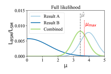
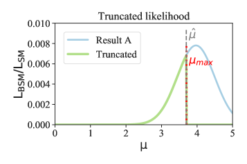
Figure 1: Left: an illustration of the signal likelihood as a function of the signal strength ($\mu$) for two results (A and B) and the corresponding combined likelihood. The value of $\hat{\mu}$ given by the maximum of the combined likelihood (green curve) is also shown as well as the upper limit on $\mu$ ($\mu_{max}$) given by Result B alone. Right: a similar example, but where it is not possible to combine both likelihoods, or the likelihood for Result B is not available. In this case the likelihood for Result A is truncated at $\mu_{max}$ (obtained from Result B). All the curves are normalized to the corresponding SM likelihood value ($\mu=0$).

5.1 Likelihoods for individual analyses

The extent to which we can compute likelihoods for individual analyses crucially depends on the information available from the experimental collaborations. Simplified-model EMs allow us to determine the expected number of events for the hypothesised proto-model. Together with the number of observed events, the expected backgrounds, and the uncertainties thereon, we can then construct a simplified likelihood by assuming a Gaussian distribution for the uncertainties and a Poissonian for the data; the nuisances are profiled over. This is a priori done per signal region. For some CMS analyses, a covariance matrix is available, which allows one to combine different signal regions, still in a simplified likelihood approach [6]. ATLAS has recently started to provide the full statistical models  [7] for some analyses, with which one can compute the likelihood at nearly  the same fidelity as in the experiment.

If only ULs are available for an analysis, things look less good. If the expected ULs are available in addition to the observed ones, we can describe the likelihood as a truncated Gaussian, although this is often a crude approximation.[1] However, if only observed ULs are available, it is simply not possible to construct a reasonable likelihood function; such results can only be used to determine $\mu_{\rm max}$ for the critic.

5.2 Combining analyses

In principle, to combine the likelihoods from individual analyses, we would need to know their correlations. Lacking this information, we treat cross-analyses correlations in an approximate, binary way—a given pair of analyses is either considered to be approximately uncorrelated, in which case it may be combined (by multiplying the respective likelihoods), or it is not at all considered for combination. We always assume results from different LHC runs and/or from different experiments to be approximately uncorrelated. Moreover, we also treat results with clearly different final states (e.g., fully hadronic final states vs. final states with leptons) to be uncorrelated. Figure 2 illustrates this for the Run 2 analyses considered in this work.

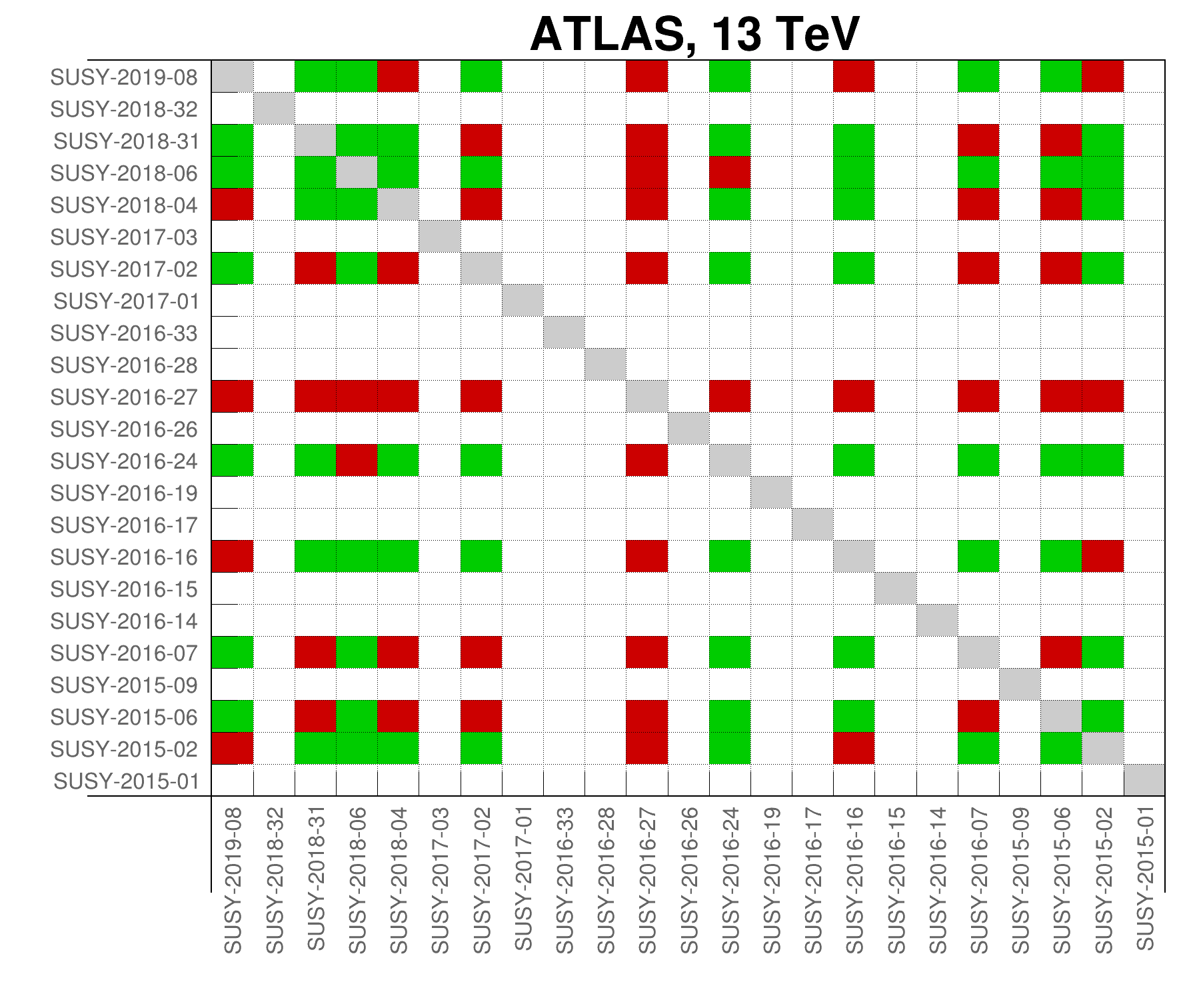
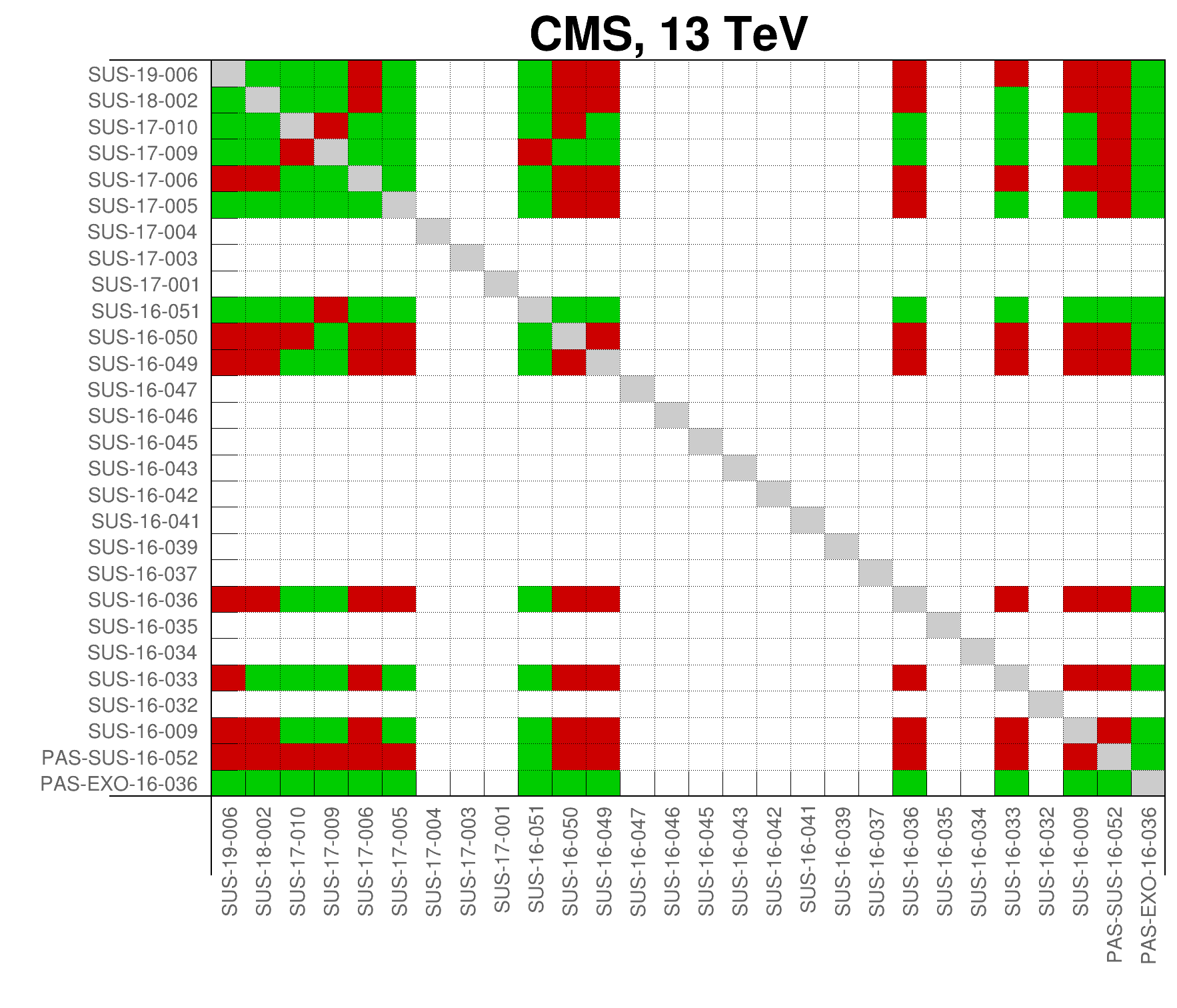
Figure 2: Binary correlation matrices for the 23 ATLAS (left) and 28 CMS (right) Run 2 analyses considered in this work, showing which ones are taken as approximately uncorrelated (green bins) and which are not (red bins). Analyses from different LHC runs or different experiments are always taken as uncorrelated. White bins denote analyses, for which no likelihood can be computed because only observed ULs are available.

With these assumptions, we construct an approximate combined likelihood for subsets of LHC results, $\mathrm{L}_{\mathbf{BSM}}(\mu)=\prod_{i=1}^{n}\mathrm{L}_{i}(\mu)$, where the product is over all $n$ uncorrelated analyses and $\mu$ is the global signal strength. We refer to such subsets as combinations of results. Two important rules apply: 1. any pair of results in the subset must be considered as uncorrelated; and 2. any result which is allowed to be added to the combination, must be added. Information from all the other analyses, which are not included in the combination, is accounted for as a constraint on the global signal strength $\mu$, i.e. $\mu_{\rm max}$.

A comment is in order at this point. Indeed, while a good number of analyses can be combined in the way described above, we also see from the white bins in Fig. 2, that about half of the Run 2 analyses in the SModelS v1.2.4 database consist of observed ULs only, and thus no proper likelihood can be computed for them. For Run 1, this concerns about one third of all analyses. Clearly, more EM-type results would be welcome to improve this situation.

6 Test statistics

Last but not least, in order to guide the MCMC-type walk and identify the proto-models that best fit the data, we need a test statistic $K$. While $K$ should increase for models which better satisfy all the constraints (which includes better fitting potential dispersed signals), it is also desirable to enforce the law of parsimony by reducing the test statistic of models with too many degrees of freedom. We define the test statistic as

$$K:=\max\limits_{\forall c\in C}K^{c}\qquad{\rm with}\qquad K^{c}=2\ln\frac{\mathrm{L}^{c}_{\mathbf{BSM}}(\hat{\mu})\cdot\pi(\mathbf{BSM})}{\mathrm{L}^{c}_{\mathbf{SM}}\cdot\pi(\mathbf{SM})}\,.$$ (2)

Here $\mathrm{L}^{c}_{\mathbf{BSM}}$ is the likelihood for a combination $c$ of experimental results given the proto-model, evaluated at the signal strength value $\hat{\mu}$, which maximizes the likelihood and satisfies $0\leq\hat{\mu}<\mu_{max}$. $\mathrm{L}^{c}_{\mathbf{SM}}$ is the corresponding SM likelihood, given by $\mathrm{L}^{c}_{\mathbf{BSM}}(\mu=0)$. Finally, $\pi(\mathbf{SM})$ and $\pi(\mathbf{BSM})$ denote respectively the priors for the SM and the proto-model. The total set of combinations of results, $C$, is determined as explained in Section 5.2.

The proto-model prior $\pi(\mathbf{BSM})$ should penalize the test statistic for newly introduced particles, branching ratios, or signal strength multipliers, while $\pi(\mathbf{SM})\equiv 1$. Here, we choose

$$\pi(\mathbf{M})=\exp\left[-\left(\frac{n_{\mathrm{particles}}}{2}+\frac{n_{\mathrm{BRs}}}{4}+\frac{n_{\mathrm{SSMs}}}{8}\right)\right]\,,$$ (3)

where $n_{\mathrm{particles}}$ is the number of new particles present in the proto-model, $n_{\mathrm{BRs}}$ is the number of non-trivial branching ratios, and $n_{\mathrm{SSMs}}$ the number of signal strength multipliers. This way, one particle with one non-trivial decay and two production modes is equivalent to one free parameter in the Akaike Information Criterion. For the SM, $n_{\mathrm{particles}}=n_{\mathrm{BRs}}=n_{\mathrm{ssm}}=0$, and $\pi(\mathbf{SM})\equiv 1$. The test statistic thus roughly corresponds to a $\Delta\chi^{2}$ of the proto-model with respect to the SM, with a penalty for the new degrees of freedom.

7 Results

For first physics results, we performed 10 runs of the walker algorithm, each employing $50$ walkers and $1,000$ steps/walker. Figure 3 displays the mass spectra of the proto-models with the highest $K$ value from each run. Besides the $X_{Z}^{1}$ as the LBP, all models include one top-partner, $X_{t}^{1}$, and one light-flavor quark partner, $X_{d,c}$, and their test statistics are at $K=6.76\pm 0.08$ thus showing the stability of the algorithm.

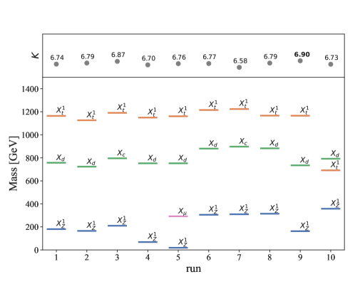
Figure 3: Particle content and masses for the proto-models with highest test-statistic $K$ obtained in each of the 10 runs performed over the real database. The corresponding $K$ values are shown at the top. Note that for all practical purposes $X_{d}$ and $X_{c}$ are indistinguishable.

For concreteness, let us take a closer look at the proto-model with $K=6.9$ from run 9. The $X_{d}$ with mass $\approx 700$ GeV is introduced in order to fit small excesses in the multijet+$E_{T}^{\rm miss}$ analyses from ATLAS at $\sqrt{s}=8$ and 13 TeV [8, 9] and from CMS at $\sqrt{s}=8$ TeV [10]. The $X_{t}^{1}$ with a mass of about $1.2$ TeV is introduced to fit the $\approx 1.5\,\sigma$ and $2\,\sigma$ excesses observed in the 13 TeV CMS and ATLAS stop searches [11, 12]; indeed this is what mostly drives the $K$ value. Despite corresponding to small excesses, identifying the presence of such potential dispersed signals is one of the main goals of the algorithm presented here. The fact that these excesses appear in distinct ATLAS and CMS analyses and can be explained by the introduction of a single top partner (actually with SUSY-like cross sections) is another interesting outcome.

Finally, we can also compute a global $p$-value for the SM hypothesis by running over synthetic “background-only” data. In the present setup, we find that $p({\rm SM})\approx 0.19$; see [1] for details.

8 Conclusions

In view of the null results (so far) in the numerous channel-by-channel searches for new particles, it becomes increasingly relevant to change perspective and attempt a more global approach to find out where BSM physics may hide. To this end, we presented a novel statistical learning algorithm that is capable of identifying potential dispersed signals in the slew of published LHC analyses. The task of the algorithm is to build candidate proto-models from small excesses in the data, while at the same time remaining consistent with all other constraints. At present, this is based on the concept of simplified models, exploiting the SModelS software framework and its large database of simplified-model results from ATLAS and CMS searches for new physics.

Acknowledgments: S.K. was supported in part by the IN2P3 project “Théorie – BSMGA”.

References

References

- [1] W. Waltenberger, A. Lessa, S. Kraml, Artificial Proto-Modelling: Building Precursors of a Next Standard Model from Simplified Model Results, JHEP 03 (2021) 207 [2012.12246].
- [2] S. Kraml et al., SModelS: a tool for interpreting simplified-model results from the LHC and its application to supersymmetry, Eur. Phys. J. C 74 (2014) 2868 [1312.4175].
- [3] F. Ambrogi et al., SModelS v1.1 user manual: Improving simplified model constraints with efficiency maps, Comput. Phys. Commun. 227 (2018) 72 [1701.06586].
- [4] F. Ambrogi et al., SModelS v1.2: long-lived particles, combination of signal regions, and other novelties, Comput. Phys. Commun. 251 (2020) 106848 [1811.10624].
- [5] G. Alguero et al., New developments in SModelS, PoS TOOLS2020, 022 [2012.08192].
- [6] CMS collaboration, Simplified likelihood for the re-interpretation of public CMS results, Tech. Rep. CMS-NOTE-2017-001.
- [7] ATLAS Collaboration, Reproducing searches for new physics with the ATLAS experiment through publication of full statistical likelihoods, Tech. Rep. ATL-PHYS-PUB-2019-029.
- [8] ATLAS collaboration, Search for squarks and gluinos with the ATLAS detector in final states with jets and missing transverse momentum using TeV proton–proton collision data, JHEP 09 (2014) 176 [1405.7875].
- [9] ATLAS collaboration, Search for squarks and gluinos in final states with jets and missing transverse momentum using 36 fb-1 of TeV collision data with the ATLAS detector, Phys. Rev. D 97 (2018) 112001 [1712.02332].
- [10] CMS collab., Search for new physics in the multijet and missing transverse momentum final state in proton-proton collisions at TeV, JHEP 06 (2014) 055 [1402.4770].
- [11] CMS collaboration, Search for supersymmetry in proton-proton collisions at 13 TeV using identified top quarks, Phys. Rev. D 97 (2018) 012007 [1710.11188].
- [12] ATLAS collaboration, Search for top-squark pair production in final states with one lepton, jets, and missing transverse momentum using 36 fb-1 of TeV collision data with the ATLAS detector, JHEP 06 (2018) 108 [1711.11520].