Optimal Control of the SIR Model with Constrained Policy, with an Application to COVID-19

Abstract

This article considers the optimal control of the SIR model with both transmission and treatment uncertainty. It follows the model presented in Gatto and Schellhorn (2021). We make four significant improvements on the latter paper. First, we prove the existence of a solution to the model. Second, our interpretation of the control is more realistic: while in Gatto and Schellhorn the control $\alpha$ is the proportion of the population that takes a basic dose of treatment, so that $\alpha>1$ occurs only if some patients take more than a basic dose, in our paper, $\alpha$ is constrained between zero and one, and represents thus the proportion of the population undergoing treatment. Third, we provide a complete solution for the moderate infection regime (with constant treatment). Finally, we give a thorough interpretation of the control in the moderate infection regime, while Gatto and Schellhorn focussed on the interpretation of the low infection regime. Finally, we compare the efficiency of our control to curb the COVID-19 epidemic to other types of control.

1 Introduction

This article extends the analysis of the model presented in Gatto and Schellhorn (2021).We make four significant improvements on the latter paper. First, we prove existence of a solution. Second, In Gatto and Schellhorn (2021) the optimal control $\alpha$ has the interpretation of the proportion of the population that takes a basic dose of treatment, so that $\alpha>1$ occurs only if a proportion of the population takes more than a basic dose of treatment. In the low infection regime part of our paper, $\alpha$ is constrained to be between zero and one, and represents thus the proportion of the population undergoing treatment. The latter interpretation is much more realistic, as it is uncommon to ration treatment. Third, we provide a complete solution for the moderate infection regime (with constant treatment). The final improvement is a thorough numerical analysis and sensitivity analysis of the moderate infection regime, while Gatto and Schellhorn (2021) focused exclusively on the interpretation of the control in the low infection regime. This enables us to discover some errors in the second-order term of the solution in Gatto and Schellhorn (2021), which we correct here. Finally, we compare the efficiency of our control to curb the COVID-19 pandemic to other types of control. While our solution is complex, it allows to satisfy the objective better. Also, our analytical solutions allow for an intuitive understanding of the optimal control compared to a purely numerical solution.

The structure of the article is as follows. In section 2 we briefly introduce the model in Gatto and Schellhorn (2021), and provide a proof of existence of the solution. In section 3, we show our results for the low infection regime. In section 4, we extend and analyze the solution in the moderate infection regime. Section 5 shows our experimental results when applying our methodology to the COVID-19 in the US in 2020. We draw the conclusion in Section 6. We refer the reader to our earlier paper, Gatto and Schellhorn (2021) for a literature review.

2 A Stochastic SIR Model with Treatment Uncertainty

Let $S$, $I$, $R$ be the proportions of susceptible, infected, and out of infection (recovered, and dead), respectively. Let $\beta$ be the transmission rate and $\mu$ be the death rate.

In the SIR model, the rate of decrease $\frac{dS}{dt}$ of the proportion of susceptible is equal to the constant transmission rate $\beta$ time $SI$. As in Gatto and Schellhorn (2021), we add a term $\sigma_{S}\sqrt{SI}\frac{dB_{1}}{dt}$, where $\frac{dB_{1}}{dt}$ is white noise, in order to model the error in the transmission rate:

$$\frac{dS}{dt}=-\beta SI+\sigma_{S}\sqrt{SI}\frac{dB_{1}}{dt}$$

The optimal policy $\alpha$ is the proportion of the infected population that received treatement, thus $\alpha(t)\in[0,1]$. The presence of this constraint is an important addition to the model in Gatto and Schellhorn (2021). Depending whether the individual is treated or not, there are then four different ways for an infected individual to exit the pool of infected:

• not treated and recover

• not treated and die

• treated and recover

• treated and died.

Thus, the ”out of infection rate” will be:

$$\begin{aligned} \frac{dR(t)}{dt}=&\underset{\text{not treated and recover}}{\underbrace{(1-\alpha(t))I(t)K_{0}}}+\underset{\text{not treated and die}}{\underbrace{(1-\alpha(t))I(t)\mu_{0}}}+\underset{\text{treated and recover}}{\underbrace{\alpha(t)I(t)K_{1}(t)}}\\ &+\underset{\text{treated and die}}{\underbrace{\alpha(t)I(t)\mu_{1}}}-\underset{\text{treatment measurement error}}{\underbrace{\alpha(t)I(t)\sigma\frac{dB_{2}}{dt}}}\end{aligned}$$ (1)

For simplicity, we assume that the Brownian motion driving transmission uncertainty ($B_{1}$) is independent from the Brownian motion driving treatment uncertainty ($B_{2}$). We suppose that $\mu_{0}\geq\mu_{1}$ (people die faster without treatment than with treatment), but the reader will not lose any intuition by supposing that $\mu_{0}=\mu_{1}$. Most of the time $K_{1}(t)>K_{0}$ (treatment is better than no treatment), but not necessarily. We relax this requirement somewhat by requiring:

$$P(K_{0}<K_{1}(t))\text{ is close to one}$$ (2)

We model the treatment rate as an Ornstein-Uhlenbeck process:

$$dK_{1}(t)=\lambda_{k}(\bar{k}_{1}-K_{1}(t))dt+\sigma_{k}dB_{2}(t)$$

with the mean-reversion rate $\lambda_{k}>0$ and the long run value of the treatment rate $\bar{k}_{1}$. It is well-known that $K_{1}$ is Gaussian, with variance equal to:

$$\mathbb{V}ar[K_{1}(t)]=\frac{\sigma_{k}^{2}}{2\lambda_{k}}(1-e^{-2\lambda_{k}t})$$

Thus, if mean-reversion is large compared to volatility $\sigma_{k}$, constraint (2) is satisfied. We simplify (1) by:

$$\frac{\frac{dR(t)}{dt}}{I(t)}=K_{0}+\mu_{0}+\alpha(t)(-K_{0}+K_{1}(t)-\mu_{0}+\mu_{1})-\alpha(t)\sigma\frac{dB_{2}}{dt}$$

Putting everything together, the dynamics of the infected is:

$$\frac{dI(t)}{dt}=\beta S(t)I(t)-\frac{dR(t)}{dt}-\sigma_{S}\sqrt{S(t)I(t)}\frac{dB_{1}}{dt}$$

We try to minimize a measure of the infected over our horizon $T$. To model risk-aversion to unfavorable treatment decisions, the decision-maker is supposed to minimize the expected value of a convex and increasing function of $I(T)$. Alternately, one can maximize the negative thereof, i.e., maximize the expected value of a concave and decreasing function of $I(T).$ Such a function $U$ is called a utility function in financial economics. The policy obtained in maximizing the expected value of a concave utility function can be showed, under certain conditions, to maximize the expected value of the outcome (here $-I$) under a constraint on the dispersion of the outcome. Out of the universe of concave decreasing utility functions, we choose the power utility function:

$$U(I)=-\frac{I^{1-\gamma}}{1-\gamma}$$

The coefficient $\gamma$ is often called the risk-aversion parameter. When $\gamma=0$ the decision-maker is risk-neutral, meaning that the uncertainty does not have an influence on her decisions. It is straightforward to check that this power utility function is concave in $I$ when $\gamma<0,$which we will assume. Taking for instance $\gamma=-1$, we see that the objective is to

$$\max\mathbb{E}\big{[}-\frac{I^{2}}{2}\big{]}$$

which returns the same policy as:

$$\min\mathbb{E}\big{[}\frac{I^{2}}{2}\big{]}$$

The importance of analytic formulations is that other figures of interest in this model, like the expected number of deaths from treatment can be analytically calculated, and depend on $\gamma$. Thus, a decision-maker can calibrate its risk-aversion parameter $\gamma$ on other goals. Expected number of deaths is only one type of goal and economic factors that can be easily added. We define

$$\tau=\min\{t>0|I(t)\leq 0\text{ or }I(t)\geq 1\}$$

Our controlled SIR model is thus:

$$\hskip 56.9055pt\sup_{0\leq\alpha(t)\leq 1}\mathbb{E}\big{[}-\frac{I(\min(\tau,T))^{1-\gamma}}{1-\gamma}\big{]}$$

$$dS(t)=-\beta S(t)I(t)dt+\sigma_{S}\sqrt{S(t)I(t)}dB_{1}(t)$$ (3)

$$dI(t)=\left(\beta S(t)-(K_{0}+\mu_{0})+\alpha(t)(K_{0}-K_{1}(t)+\mu_{0}-\mu_{1})\right)I(t)dt$$

$$~{}~{}~{}~{}~{}~{}~{}~{}~{}+\alpha(t)I(t)\sigma dB_{2}(t)-\sigma_{S}\sqrt{S(t)I(t)}dB_{1}(t)$$ (4)

$$dK(t)=\lambda_{k}(\bar{K}-K(t))dt+\sigma_{k}dB_{2}(t)$$ (5)

The relative sign of our volatilities $\sigma$ and $\sigma_{k}$ is important. We will assume without loss of generality that $\sigma<0$. The sign of $\sigma_{k}$ is the sign of covariance between the measured value of today’s treatment rate and the change in value of the treatment rate between today and a future date. An example may help illustrate the difference. Suppose that over a week one performs daily measurements of the treatment recovery rate as well as daily forecasts of the evolution of the treatment recovery rate over the next day. The two quantities measured each day $t$ are proportional to the same white noise $B_{2}(t+$1 day$)-B_{2}(t)$. One then calculates weekly estimates $\hat{\sigma}$ of $\sigma$ and $\hat{\sigma}_{k}$ of $\sigma_{k}$ over these 7 daily observations. Since we arbitrarily choose $\sigma>0$, a positive $\hat{\sigma}_{k}$ shows a correlation of +1 between the measurement (of today’s treatment rate) and the forecast. Figure 1 is a depiction of our model.

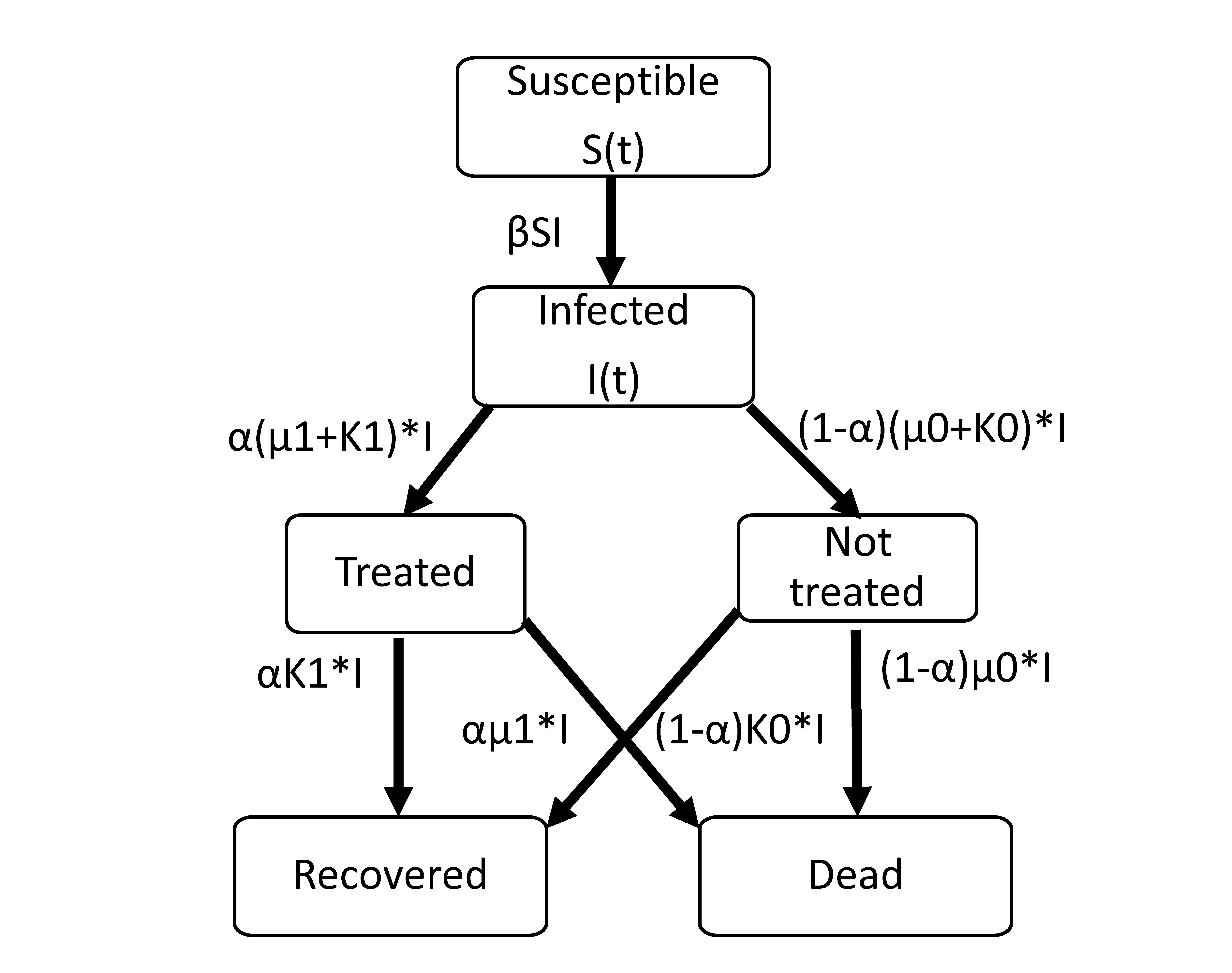
Figure 1: A stochastic SIR model

Theorem 1.

For any given intial value $(S(0),I(0),R(0))$ and any $X(0)$ there exists a unique solution of (3)(4)(5) up to time $\tau$.

The proof of Theorem 1, included in Appendix A, follows the proof of a theorem of Yamada and Watanabe (1971), as exposed in the book by Karatzas and Shreve (2014, Prop. 2.13, Sec. 5.2).

3 Results in the Low Infection Regime

We assume $S(t)$ close to one and $\sigma_{S}=0$. Thus the term:

$$r=\beta S(t)-(K_{0}+\mu_{0})\simeq\beta-K_{0}-\mu_{0}$$

is assumed constant. With this simplification, we give an analytical solution to the constrained problem, i.e., the case where $0\leq\alpha(t)\leq 1$, a significant improvement over Gatto and Schellhorn, who considered the unconstrained case.

We define the impact of treatment risk $X$:

$$X(t)=\frac{K_{0}+\mu_{0}-\mu_{1}-K_{1}(t)}{\sigma}$$

as well as the long run impact of the treatment risk $\bar{X}$:

$$\bar{X}=\frac{K_{0}+\mu_{0}-\mu_{1}-\bar{k}_{1}}{\sigma}$$

We define $\lambda_{x}=\lambda_{k}$ and $\sigma_{x}=\sigma_{k}/\sigma$. For simplicity we write $\mu=K_{0}+\mu_{0}$. We consider first the case where the treatment rate is constant, and then the case where it follows an Ornstein Uhlenbeck process.

3.1 Constant Treatment Rate

Let $b=\beta-\mu_{1}-\bar{k}_{1}$. The problem is:

$$\begin{gathered}\sup_{0\leq\alpha(t)\leq 1}\mathbb{E}\big{[}-\frac{I(T)^{1-\gamma}}{1-\gamma}\big{]}\\ dI(t)=(r+\alpha(t)(b-r))I(t)dt+\alpha(t)\sigma I(t)dB_{2}(t)\end{gathered}$$ (6)

Theorem 2.

The optimal control is constant, and satisfies

$$\alpha=\min\Big{(}1,\max\big{(}0,\frac{\bar{k}_{1}-K_{0}}{\sigma^{2}|\gamma|}\big{)}\Big{)}$$

The proof is the Appendix B, and follows closely Cvitanić and Karatzas (1992).

3.2 Treatment Rate as Ornstein-Uhlenbeck Process

The problem is

$$\begin{aligned} &\hskip 56.9055pt\sup\mathbb{E}\big{[}-\frac{I(T)^{1-\gamma}}{1-\gamma}\big{]}\\ &dI(t)=(r+\alpha(t)\sigma X(t))I(t)dt+\alpha(t)\sigma I(t)dB_{2}(t)\\ &dX(t)=\lambda_{x}(\bar{X}-X(t))dt-\sigma_{x}dB_{2}(t)\end{aligned}$$ (7)

In the low infection regime our solution will depend on a kernel $H_{0}(X_{t},\tau)$ with $\tau=T-t$, while in the moderate infection regime it will also depend on two other kernels $H_{1}(X_{t},\tau)$ and $H_{2}(X_{t},\tau)$ that are closely related. In order to unify notation we define the kernels. Define

$$H_{0}(X_{t},\tau)=\exp\left(\frac{1}{\gamma}\Big{(}\frac{A_{1}(\tau,\gamma)X_{t}^{2}}{2}+A_{2}(\tau,\gamma)X_{t}+A_{3}(\tau,\gamma)+(1-\gamma)(\mu+r)\tau\Big{)}\right)$$ (8)

and, for $i>0$

$$H_{i}(X_{t},\tau)=\exp\left(\frac{i}{\gamma}\Big{(}\frac{A_{1}(\tau,\gamma/i)X_{t}^{2}}{2}+A_{2}(\tau,\gamma/i)X_{t}+A_{3}(\tau,\gamma/i)\Big{)}\right)$$ (9)

where

$$A_{1}(\tau,\gamma)=\frac{1-\gamma}{\gamma}\frac{2(1-\exp(-\theta(\gamma)\tau))}{2\theta(\gamma)-(b_{2}(\gamma)+\theta(\gamma))(1-\exp(-\theta(\gamma)\tau))}$$ (10)

$$A_{2}(\tau,\gamma)=\frac{4\lambda_{x}\bar{X}b_{1}(\gamma)\left(1-\exp\left(-\theta(\gamma)\tau/2\right)\right)^{2}}{\theta(\gamma)\left(2\theta(\gamma)-(\theta(\gamma)+b_{2}(\gamma))(1-\exp(-\theta(\gamma)\tau))\right)}$$ (11)

$$A_{3}(\tau,\gamma)=\int_{0}^{\tau}\left(\frac{\sigma_{x}^{2}}{2\gamma}+\lambda_{x}\bar{X}\right)A_{2}^{2}(s,\gamma)+\frac{\sigma_{x}^{2}}{2}A_{1}(s,\gamma)+(\gamma-1)\mu ds$$ (12)

$$b_{1}(\gamma)=\frac{1-\gamma}{\gamma}~{}~{}~{}~{}~{}b_{2}(\gamma)=2\big{(}\frac{\gamma-1}{\gamma}\sigma_{x}-\lambda_{x}\big{)}~{}~{}~{}~{}~{}b_{3}(\gamma)=\frac{\sigma_{x}^{2}}{\gamma}$$

$$\theta(\gamma)=\sqrt{b_{2}^{2}(\gamma)-4b_{1}(\gamma)b_{3}(\gamma)}$$

We provide an explicit formula for $A_{3}(\tau,\gamma)$ in Appendix C. The solution to (7) is shown in Gatto and Schellhorn (2021, Prop. 1), but with some typos in the expression of $H_{0}(X_{t},\tau)$, hence we correct the mistake by providing (8) in this paper.

4 Results in the Moderate Infection Regime

We first handle the Ornstein-Uhlenbeck treatment rate case, which was presented in Gatto and Schellhorn (2021, Prop. 2). In this work, we aim to correct the typos and provide more detials for the Proposition 2 in Gatto and Schellhorn (2021).

4.1 Treatment Rate as Ornstein-Uhlenbeck Process

The problem is defined in Section 2. We rewrite here for convenience,

$$\begin{aligned} &\hskip 56.9055pt\sup\mathbb{E}\big{[}-\frac{I(\min(\tau,T))^{1-\gamma}}{1-\gamma}\big{]}\\ &dS(t)=-\beta S(t)I(t)dt+\sigma_{S}\sqrt{S(t)I(t)}dB_{1}(t)\\ &dI(t)=\left(\beta S(t)-\mu+\alpha(t)\sigma X(t)\right)I(t)dt+\alpha(t)I(t)\sigma dB_{2}(t)\\ &\hskip 28.45274pt-\sigma_{S}\sqrt{S(t)I(t)}dB_{1}(t)\\ &dX(t)=\lambda_{x}(\bar{X}-X(t))dt-\sigma_{x}dB_{2}(t)\end{aligned}$$ (13)

To express the solution of (13), we further define

$$\tilde{M}(t,\tau)=\frac{2\theta(\gamma)e^{\frac{1}{2}(b_{2}(\gamma/2)-b_{2}(\gamma)-\theta(\gamma))(\tau-t)}}{2\theta(\gamma)-(b_{2}(\gamma)+\theta(\gamma))\left(1-e^{-\theta(\gamma)(\tau-t)}\right)}$$ (14)

$$m_{Y}(\tau,x)=x\tilde{M}(t,\tau)+\int_{s=t}^{\tau}\tilde{M}(s,\tau)(\lambda_{x}\bar{X}+\frac{\sigma_{x}^{2}}{{}^{\gamma}}A_{2}(\tau-s,\gamma))ds$$

$$\hskip 56.9055pt+\frac{A_{2}(T-\tau,\gamma)}{A_{1}(T-\tau,\gamma)}$$

$$V_{Y}(\tau,x)=\sigma_{x}^{2}\int_{t}^{\tau}\tilde{M}^{2}(s,\tau)ds$$

$$g(X,t)=\int_{\tau=t}^{T}H_{2}(X,\tau-t)\frac{1}{2}\frac{\beta^{2}}{\sigma_{S}^{2}\gamma}\frac{1}{\sqrt{1-2V_{Y}(\tau,X)A_{1}(T-\tau,\gamma)/\gamma}}$$

$$\hskip 42.67912pt\times\exp\Big{(}\frac{2}{\gamma}A_{3}(T-\tau,\gamma)-\frac{A_{2}^{2}(T-\tau,\gamma)}{\gamma A_{1}(T-\tau,\gamma)}$$ (15)

$$\hskip 85.35826pt+\frac{m_{Y}^{2}(\tau,X)A_{1}(T-\tau,\gamma)}{\gamma-2V_{Y}(\tau,X)A_{1}(T-\tau,\gamma)}\Big{)}d\tau$$

From this, we can calculate:

$$\frac{\partial g}{\partial X}=\int_{\tau=t}^{T}H_{2}(X,\tau-t)\frac{1}{2}\frac{\beta^{2}}{\sigma_{S}^{2}\gamma}\frac{1}{\sqrt{1-2V_{Y}(\tau,X)A_{1}(T-\tau,\gamma)/\gamma}}$$

$$\times\exp\left(\frac{2}{\gamma}A_{3}(T-\tau,\gamma)-\frac{A_{2}^{2}(T-\tau,\gamma)}{\gamma A_{1}(T-\tau,\gamma)}+\frac{m_{Y}^{2}(\tau,X)A_{1}(T-\tau,\gamma)}{\gamma-2V_{Y}(\tau,X)A_{1}(T-\tau,\gamma)}\right)$$

$$\times\Big{(}\frac{A_{1}(\tau-t,\gamma/2)X(t)+A_{2}(\tau-t,\gamma/2)}{\gamma/2}$$

$$\hskip 85.35826pt+\frac{2m_{Y}(\tau,X)A_{1}(T-\tau,\gamma)}{\gamma-2V_{Y}(\tau,X)A_{1}(T-\tau,\gamma)}\tilde{M}(t,\tau)\Big{)}d\tau$$

Theorem 3.

Let $I(0)=\varepsilon$. Suppose $I(t)\leq 1$. If $\sigma_{x}<0$ then the problem (13) has a solution such that

$$I(t)=\varepsilon Z^{1/\gamma}(t)H_{1}(X(t),T-t)+\varepsilon^{2}Z^{2/\gamma}(t)S(t)g(X(t),t)+O(\varepsilon^{3})$$

where $Z(t)$ satisfies:

$$\frac{dZ}{Z}=(-\mu+X^{2}+\frac{\beta^{2}SI}{\sigma_{S}^{2}})dt-\frac{\beta\sqrt{SI}}{\sigma_{S}}dB_{1}+XdB_{2}$$

$$Z(0)=\left(\frac{-H_{1}(X(0),T)+\sqrt{H_{1}^{2}(X(0),T)-4\varepsilon S(0)g(X(0),0)(\mathcal{O}(\varepsilon^{2})-1)}}{2\varepsilon S(0)g(X(0),0)}\right)^{\gamma}$$

The optimal control $\alpha^{\ast}(t)=\alpha_{0}(t)+\varepsilon\alpha_{1}(t)+\mathcal{O}(\varepsilon^{2})$ where:

$$\alpha_{0}(t)=\frac{X(t)}{\gamma\sigma}-\frac{\sigma_{x}}{\gamma\sigma}\left(A_{1}(T-t,\gamma)X(t)+A_{2}(T-t,\gamma)\right)$$

$$\alpha_{1}(t)=\frac{Z^{1/\gamma}(t)S(t)}{H_{1}(X(t),T-t)\sigma}\Big{(}\frac{g(X(t),t)X(t)}{\gamma}-\sigma_{x}\frac{\partial g}{\partial X}$$

$$\hskip 28.45274pt+\sigma_{x}\frac{g(X(t),t)}{\gamma}\left(A_{1}(T-t,\gamma)X(t)+A_{2}(T-t,\gamma)\right)\Big{)}$$

The proof is in Appendix D. We refer to Gatto and Schellhorn (2021) for a discussion of $\alpha_{0}$. The sign of $\alpha_{1}$ is determined by the signs of $\sigma$ and

$$\frac{g(X(t),t)}{\gamma}\Big{(}X(t)+\sigma_{x}\left(A_{1}(T-t,\gamma)X(t)+A_{2}(T-t,\gamma)\right)\Big{)}-\sigma_{x}\frac{\partial g}{\partial X}$$ (16)

More specifically, $\alpha_{1}$ is positive if $\sigma$ and (16) are both positive or negative. $\alpha_{1}$ is negative if one of them is positive and the other one is negative.

It is obvious that the magnitude of both $g(X(t),t)$ and $\frac{\partial g}{\partial X}$ decrease with time and are equal to zero when $t=T$. Therefore, the importance of $\alpha_{1}$ decreases as time increases.

To further discuss the sign of (16), we rewrite it by

$$\left|\frac{g(X(t),t)}{\gamma}\right|\left(\left(1+\left|\sigma_{x}A_{1}(T-t,\gamma)\right|\right)X(t)+\bar{X}\left|\frac{\sigma_{x}A_{2}(T-t,\gamma)}{\bar{X}}\right|\right)+|\sigma_{x}|\frac{\partial g}{\partial X}$$

Thus, suppose $\frac{\partial g}{\partial X}$, $X(t)$, and $\bar{X}$ are all positive, (16) is positive, and vice versa. In the following cases, we provide two simple cases that we can easily discuss the sign of $\alpha_{1}$:

• if $\frac{\partial g}{\partial X}\sigma>0$, $\mu-\mu_{1}>\max(K_{1}(t),\bar{k}_{1})$, then $\alpha_{1}$ is positive.

• if $\frac{\partial g}{\partial X}\sigma<0$, $\mu-\mu_{1}<\min(K_{1}(t),\bar{k}_{1})$, then $\alpha_{1}$ is negative.

In the following, we discuss the full expansion of the solution in Theorem 3. Consider equation (57) in Gatto and Schellhorn (2021):

$$\Big{(}\frac{\partial}{\partial t}+L_{1}+\varepsilon L_{2}\Big{)}f=0$$

This time we use full asymptotic expansion:

$$f=f_{1}+\varepsilon f_{2}+\ldots=\sum_{i=1}^{\infty}f_{i}\varepsilon^{i-1}$$

and obtain:

$$0 = \Big{(}\frac{\partial}{\partial t}+L_{1}\Big{)}f_{1}+\sum_{i=1}^{\infty}\Big{(}\Big{(}\frac{\partial}{\partial t}+L_{1}\Big{)}f_{i+1}+L_{2}f_{i}\Big{)}\varepsilon^{i}$$

The terms of our asymptotic expansion are thus determined by:

$$\Big{(}\frac{\partial}{\partial t}+L_{1}\Big{)}f_{1}=0$$ (17)

$$\Big{(}\frac{\partial}{\partial t}+L_{1}\Big{)}f_{i+1}=-L_{2}f_{i}~{}~{}~{}~{}~{}~{}i=1,2,\ldots$$ (18)

We use the Ansatz:

$$f_{i}(Z(t),X(t),t)=Z(t)^{2^{i-1}/\gamma}S(t)^{2^{i-1}-1}g_{i}(X(t),t)~{}~{}~{}~{}~{}~{}i=1,2,\ldots$$

We have showed that $g_{1}=H_{1}$ and $g_{2}=g$ in the proof of Theorem 3. By the same process, we can also calculate the expressions for $g_{3}$, $g_{4},\ldots$ in the sequel.

4.2 Constant Treatment Rate

The problem is:

$$\begin{aligned} &\hskip 56.9055pt\sup\mathbb{E}\big{[}-\frac{I(T)^{1-\gamma}}{1-\gamma}\big{]}\\ &dS(t)=-\beta S(t)I(t)dt+\sigma_{S}\sqrt{S(t)I(t)}dB_{1}(t)\\ &dI(t)=(r+\alpha(t)(b-r))I(t)dt+\alpha(t)\sigma I(t)dB_{2}(t)-\sigma_{S}\sqrt{S(t)I(t)}dB_{1}(t)\end{aligned}$$ (19)

Let $\tau=T-t$, the solution kernels $h_{i}(\tau)$ for $i=1,2,\ldots$ are given by:

$$h_{i}(\tau)=\exp\Big{(}\frac{2^{i-1}}{\gamma}\Big{(}\frac{a_{i,1}}{2}\big{(}\frac{b-r}{\sigma}\big{)}^{2}+a_{i,2}\Big{)}\tau\Big{)}$$ (20)

where

$$a_{i,1} = \frac{1-\gamma/2^{i-1}}{\gamma/2^{i-1}}$$ (21)

$$a_{i,2} = (\gamma/2^{i-1}-1)\mu$$ (22)

Theorem 4.

Let $I(0)=\varepsilon$, then the problem (19) has a solution such that

$$I(t)=\sum_{i=1}^{\infty}Z(t)^{2^{i-1}/\gamma}S(t)^{2^{i-1}-1}g_{i}(t)\varepsilon^{i}$$

where $g_{1}(t)=h_{1}(T-t)$, $g_{i}(t)$, $i>1$ can be obtained by (45), and $Z(t)$ satisfies:

$$\frac{dZ}{Z}=\Big{(}-\mu+\big{(}\frac{b-r}{\sigma}\big{)}^{2}+\frac{\beta^{2}SI}{\sigma_{S}^{2}}\Big{)}dt-\frac{\beta\sqrt{SI}}{\sigma_{S}}dB_{1}+\frac{b-r}{\sigma}dB_{2}$$

$$1=\sum_{i=1}^{\infty}Z(0)^{2^{i-1}/\gamma}S(0)^{2^{i-1}-1}g_{i}(0)\varepsilon^{i-1}$$

Moreover the optimal proportion undergoing treatment $\alpha^{\ast}(t)$ equal to $\alpha_{0}(t)+\varepsilon\alpha_{1}(t)+\mathcal{O}(\varepsilon^{2})$, where $\alpha_{0}(t)$ and $\alpha_{1}(t)$ are equal to

$$\alpha_{0}=\frac{b-r}{\gamma\sigma^{2}}~{}~{}~{}~{}~{}~{}~{}~{}\alpha_{1}=\frac{Z^{1/\gamma}(t)S(t)}{h_{1}(T-t)g_{2}(t)}\frac{b-r}{\gamma\sigma^{2}}$$

The proof is in Appendix E, where we also provide a formula for $g_{3}$. Observe that

$$g_{2}(t)=\frac{\beta^{2}}{2\sigma_{S}^{2}}\frac{h_{2}(T-t)-h_{1}^{2}(T-t)}{\big{(}\frac{b-r}{\sigma}\big{)}^{2}(a_{1,1}-a_{2,1})+2(a_{1,2}-a_{2,2})}=\frac{\beta^{2}}{2\sigma_{S}^{2}}\frac{h_{2}(T-t)-h_{1}^{2}(T-t)}{\gamma\mu-\big{(}\frac{b-r}{\sigma}\big{)}^{2}/\gamma}$$

is always positive because the signs of $h_{2}(T-t)-h_{1}^{2}(T-t)$ and $\gamma\mu-\big{(}\frac{b-r}{\sigma}\big{)}^{2}/\gamma$ are the same. The signs of $\alpha_{0}$ and $\alpha_{1}$ are determined by the sign of $\frac{r-b}{\sigma^{2}}$.

5 Application to COVID-19

We use the same data set and parameters (see Table 1) as in Gatto and Schellhorn (2021), but this time we show the optimal control (result of Theorem 2) of problem (6).

Treatment Parameter	Symbol	Value
Death rate/no treatment	$\mu_{0}$	0.0575
Death rate	$\mu_{1}$	0.0575
Recovery rate/ no treatment	$K_{0}$	0.2559
Recovery rate at time 0	$K_{1}(0)$	0.2559
Long run value of recovery rate	$\bar{k}_{1}$	0.4612
Volatility of the measurement of today’s recovery rate	$\sigma$	0.4418
Volatility of changes in the recovery rate	$\sigma_{k}$	-1.1647
Speed of mean-reversion of the recovery rate	$\lambda_{k}$	0.7692
Transmission rate	$\beta$	0.025
Proportion of infected at time 0	$\varepsilon$	0.01
Time step	$\Delta t$	0.001

Table 1: Parameters

We compare in Figure 2 three types of treatment:

• no treatment

• full control, i.e., $\alpha(t)=1$

• optimal control, given in Theorem 2

We can see that, for all risk-aversion parameters $\gamma$ considered (between $-1$ and $-5$), our control is better.

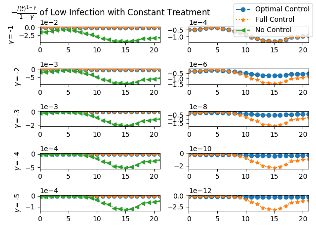
Figure 2: Optimal control of low infection with constant treatment. Weekly US COVID-19 data from June 7, 2020 to November 1, 2020. Github repository for generating the plot: https://github.com/yujiading/optimal-control-sir-model.

6 Conclusion

We showed that a stochastic optimal control approach enables to fight the COVID-19 epidemic better. Many interesting problems remain to be solved. For instance, we could analytic constrained policies in the multiple treatment case or the Ornstein-Uhlenbeck case. Optimal vaccination is another area where we believe a similar asymptotic approach can be used. Finally, Bertozzi et al. (2020) use Hawkes processes to model COVID-19. The control of Hawkes processes remains a largely open problem that deserves attention, in particular for its application to epidemiology.

Appendix A Proof of Theorem 1

We follow the proof in Karatzas and Shreve (2014, Prop. 2.13, Sec. 5.2). They consider the one-dimensional case. Let $h:[0,\infty)\rightarrow[0,\infty)$ be a strictly increasing function with $h(0)$ and

$$\int_{(0,\varepsilon)}h^{-2}(u)=\infty\text{, \ \ }\forall\varepsilon>0$$ (23)

In our case, we take $h(x)=x$.  Because of (23), there exists a strictly decreasing sequence $\{a_{n}\}\subset(0,1]$ with $a_{0}$ and $\lim_{n\rightarrow\infty}a_{n}=0$ such that $\int_{a_{n}}^{a_{n-1}}h^{-2}(u)du=n$. For every $n$ there exists continuous function $\rho_{n}$ on $\mathbb{R}$ with support on $(a_{n},a_{n-1})$ so that

$$0\leq\rho_{n}(x)\leq\frac{2}{nh(x)}\text{, \ \ }x>0$$

and $\int_{a_{n-1}}^{a_{n}}\rho_{n}(u)du=1$. Then the function

$$\Psi_{n}(x)=\int_{0}^{|x|}\int_{0}^{y}\rho_{n}(u)dudy$$

is even and twice continuously differentiable, with $|\Psi_{n}^{\prime}(x)|\leq 1$ and $\lim_{n\rightarrow\infty}$ $\Psi_{n}(x)$ $=|x|$. Suppose there are two strong solutions $(I^{(1)},S^{(1)})$ and $(I^{(2)},S^{(2)})$,

$$d(I^{(1)}-I^{(2)}-\mathbb{E}[I^{(1)}-I^{(2)}])-\alpha\sigma(I^{(1)}-I^{(2)})dB_{2}$$

$$~{}~{}~{}=-\sigma_{S}\left(\sqrt{S^{(1)}I^{(1)}}-\sqrt{S^{(2)}I^{(2)}}\right)dB_{1}$$

$$~{}~{}~{}=-d(S^{(1)}-S^{(2)}-\mathbb{E}[S^{(1)}-S^{(2)}])$$

so that

$$(d(I^{(1)}-I^{(2)}))^{2}<\sigma_{S}^{2}(S^{(1)}I^{(1)}-S^{(2)}I^{(2)})dt+(\alpha\sigma)^{2}(I^{(1)}-I^{(2)})^{2}dt$$

$$(d(S^{(1)}-S^{(2)}))^{2}<\sigma_{S}^{2}(S^{(1)}I^{(1)}-S^{(2)}I^{(2)})dt$$

$$d((I^{(1)}-I^{(2)})(S^{(1)}-S^{(2)}))<-\sigma_{S}^{2}(S^{(1)}I^{(1)}-S^{(2)}I^{(2)})dt$$

Thus, since $|\Psi_{n}^{\prime}|<1$,

$$\mathbb{E}[d\Psi_{n}(I_{t}^{(1)}-I_{t}^{(2)})+d\Psi_{n}(S_{t}^{(1)}-S_{t}^{(2)})]$$

$$~{}~{}~{}=\mathbb{E}[\Psi_{n}^{\prime}(I_{t}^{(1)}-I_{t}^{(2)})(d(I^{(1)}-I^{(2)}))+\Psi_{n}^{\prime}(S_{t}^{(1)}-S_{t}^{(2)})(d(S^{(1)}-S^{(2)}))]$$

$$~{}~{}~{}~{}~{}~{}+\frac{1}{2}\mathbb{E}[\Psi_{n}^{\prime\prime}(I_{t}^{(1)}-I_{t}^{(2)})(d(I^{(1)}-I^{(2)}))^{2}]$$

$$~{}~{}~{}~{}~{}~{}+\frac{1}{2}\mathbb{E}[\Psi_{n}^{\prime\prime}(S_{t}^{(1)}-S_{t}^{(2)})(d(S^{(1)}-S^{(2)}))^{2}]$$

$$~{}~{}~{}\leq\mathbb{E}[2|\beta||S^{(1)}I^{(1)}-S^{(2)}I^{(2)}|dt+|D||I^{(1)}-I^{(2)}|dt]$$

$$~{}~{}~{}~{}~{}~{}+\frac{1}{2}\mathbb{E}[\Psi_{n}^{\prime\prime}(I_{t}^{(1)}-I_{t}^{(2)})\sigma_{S}^{2}(S^{(1)}I^{(1)}-S^{(2)}I^{(2)})dt]$$

$$~{}~{}~{}~{}~{}~{}+\frac{1}{2}\mathbb{E}[\Psi_{n}^{\prime\prime}(S_{t}^{(1)}-S_{t}^{(2)})\sigma_{S}^{2}(S^{(1)}I^{(1)}-S^{(2)}I^{(2)})dt]$$

$$~{}~{}~{}~{}~{}~{}+\frac{1}{2}\mathbb{E}[\Psi_{n}^{\prime\prime}(I_{t}^{(1)}-I_{t}^{(2)})(\alpha\sigma)^{2}(I^{(1)}-I^{(2)})^{2}]dt$$

where

$$D=-(K_{0}+\mu_{0})+\alpha(K_{0}-K_{1}+\mu_{0}-\mu_{1})$$

Observe that:

$$S^{(1)}I^{(1)}-S^{(2)}I^{(2)} = S^{(1)}(I^{(1)}-I^{(2)})+I^{(2)}(S^{(1)}-S^{(2)})$$

$$< |I^{(1)}-I^{(2)}|+|S^{(1)}-S^{(2)}|$$

Since $\Psi_{n}^{\prime\prime}<2/nh$ and $h$ is positive,

$$\left(\Psi_{n}^{\prime\prime}(I_{t}^{(1)}-I_{t}^{(2)})+\Psi_{n}^{\prime\prime}(S_{t}^{(1)}-S_{t}^{(2)})\right)\left(S^{(1)}I^{(1)}-S^{(2)}I^{(2)}\right)$$

$$~{}~{}~{}<\frac{2}{n}\left(\frac{1}{h(|I^{(1)}-I^{(2)}|)}+\frac{1}{h(|S^{(1)}-S^{(2)}|)}\right)(|I^{(1)}-I^{(2)}|+|S^{(1)}-S^{(2)}|)$$

$$~{}~{}~{}<\frac{2}{n}\left(\frac{|I^{(1)}-I^{(2)}|}{h(|I^{(1)}-I^{(2)}|)}+\frac{|S^{(1)}-S^{(2)}|}{h(|S^{(1)}-S^{(2)}|)}\right)$$

Taking $h(x)=x$ results in

$$\mathbb{E}[d\Psi_{n}(I_{t}^{(1)}-I_{t}^{(2)})+d\Psi_{n}(S_{t}^{(1)}-S_{t}^{(2)})]$$

$$~{}~{}~{}<\Big{(}\mathbb{E}[(2|\beta|+|D|)|I^{(1)}-I^{(2)}|]+\mathbb{E}[2|\beta||S^{(1)}-S^{(2)}|]$$

$$~{}~{}~{}~{}~{}~{}+\frac{2\sigma_{S}^{2}}{n}+\frac{(\alpha\sigma)^{2}}{2}\mathbb{E}[|I^{(1)}-I^{(2)}|]\Big{)}dt$$

Since $\lim_{n\rightarrow\infty}\Psi_{n}(x)=|x|$,

$$\mathbb{E}[|I_{t}^{(1)}-I_{t}^{(2)}|+|S_{t}^{(1)}-S_{t}^{(2)}|]$$

$$~{}~{}~{}<\int_{0}^{t}\mathbb{E}[(2|\beta|+|D_{s}|)|I_{s}^{(1)}-I_{s}^{(2)}|]+\mathbb{E}[2|\beta||S_{s}^{(1)}-S_{s}^{(2)}|]$$

$$~{}~{}~{}~{}~{}~{}+\frac{(\alpha_{s}\sigma)^{2}}{2}\mathbb{E}[|I_{s}^{(1)}-I_{s}^{(2)}|]ds$$

But,

$$\mathbb{E}[(2|\beta|+|D_{s}|)|I_{s}^{(1)}-I_{s}^{(2)}|]<\sqrt{\mathbb{E}[(2|\beta|+|D_{s}|)^{2}]}\sqrt{\mathbb{E}[|I_{s}^{(1)}-I_{s}^{(2)}|^{2}]}$$

Since $|I_{s}^{(1)}-I_{s}^{(2)}|<1$, $\mathbb{E}[(I_{s}^{(1)}-I_{s}^{(2)})^{2}]<1$ and $\sqrt{\mathbb{E}[(I_{s}^{(1)}-I_{s}^{(2)})^{2}]}<\mathbb{E}[|I_{s}^{(1)}-I_{s}^{(2)}|]$ thus

$$\mathbb{E}[|I_{t}^{(1)}-I_{t}^{(2)}|+|S_{t}^{(1)}-S_{t}^{(2)}|]$$

$$~{}~{}~{}<\int_{0}^{t}\left(\sqrt{\mathbb{E}[(2|\beta|+|D_{s}|)^{2}]}+\frac{(\alpha\sigma)^{2}}{2}\right)\mathbb{E}[|I_{s}^{(1)}-I_{s}^{(2)}|]$$

$$~{}~{}~{}~{}~{}~{}+2|\beta|\mathbb{E}[|S_{s}^{(1)}-S_{s}^{(2)}|]ds$$

$$~{}~{}~{}<\int_{0}^{t}\max\left(\sqrt{\mathbb{E}[(2|\beta|+|D_{s}|)^{2}]}+\frac{(\alpha\sigma)^{2}}{2},2|\beta|\right)$$

$$~{}~{}~{}~{}~{}~{}\times\mathbb{E}[|I_{s}^{(1)}-I_{s}^{(2)}|+|S_{s}^{(1)}-S_{s}^{(2)}|]ds$$

and local uniqueness follows by Gronwall’s inequality.

Appendix B Proof of Theorem 2

We refer to the problem treated by Gatto and Schellhorn (2021) as the unconstrained problem. Indeed, in that problem $\alpha$ was not constrained. We refer to our problem as the constrained problem. We follow the method of proof in Cvitanić and Karatzas (1992), referred to hereafter as CK. They introduce auxiliary problems, which are unconstrained. They show that there exists an auxiliary problem which solution can be used to construct the solution of the original constrained problem. We follow the numbering of the sections in CK in order to ease understanding.

CK Section 2. The Model.

To ease the correspondence with the CK paper, we define $b-r=K_{0}+\mu_{0}-\mu_{1}-\bar{k}_{1}$, $\theta:=(b-r)/\sigma$, and

$$H^{(0)}(t)=\exp(-rt)\exp\Big{(}-\int_{0}^{t}\theta dB_{2}(s)-\frac{1}{2}\int_{0}^{t}\theta^{2}ds\Big{)}$$

Observe that $\mathbb{E}[\int_{0}^{t}\theta^{2}ds]<\infty$.

CK Section 3. Portfolio and consumption processes.

Define:

$$B_{2}^{(0)}(t)=B_{2}(t)+\int_{0}^{t}\theta ds$$

Denote by $I^{i,\alpha}$ the infected process subject to $I(0)=i$ and control $\alpha$. It is admissible if

$$0\leq I^{i,\alpha}(t)\leq 1\text{ \ \ \ }\forall~{}0\leq t\leq T$$

The set of admissible $\alpha$ is denoted $\mathcal{A}_{0}(i)$. Note that (See (3.5) in CK)

$$H^{(0)}(t)I(t)=i+\int_{0}^{t}H^{(0)}(s)I(s)(\alpha(s)\sigma-\theta)dB_{2}(s)$$

CK Section 4. Convex sets and their support functions.

The difference between CK and this paper is that our objective is to minimize. This means that the key relation between our auxiliary infected and infected is reversed compared to the first equation in CK. Indeed if $\alpha_{\nu}$ solves the auxiliary problem and $\alpha$ the original problem, we must have:

$$I_{\nu}^{i,\alpha_{\nu}}(t)\leq I^{i,\alpha}(t)$$

Define

$$\delta(\nu)=\left\{\begin{array}[]{cc}0&\nu<0\\ \nu&\nu>0\end{array}\right.$$ (24)

It is subadditive:

$$\delta(\lambda+\nu)\leq\delta(\lambda)+\delta(\nu)$$ (25)

CK Section 5. Utility functions.

The main difference between our utility functions and the utility functions in financial economics is that our utility functions are decreasing for positive arguments. Recall indeed that our utility function is, for $\gamma<0$:

$$U(i)=-\frac{i^{1-\gamma}}{1-\gamma}$$

Since

$$U^{\prime}(i)=-i^{-\gamma}$$

We have $\lim_{i\rightarrow\infty}U^{\prime}(i)=-\infty$ and $\lim_{i\rightarrow 0}U^{\prime}(i)=0$, again for $\gamma<0$. This is unlike CK and Wachter (2002) who consider the case $0<\gamma<1$ with utility of wealth $U_{2}(x)=\frac{x^{1-\gamma}}{1-\gamma}$. In their case, $\lim_{x\rightarrow\infty}U_{2}^{\prime}(x)=0$ and $\lim_{x\rightarrow 0}U_{2}^{\prime}(x)=\infty$.

We define $I_{2}$ to be the inverse of $U^{\prime}$, with $I_{2}(y)$ on $y\leq 0$. By straighforward calculations:

$$I_{2}(y)=(-y)^{-1/\gamma}$$

We also define the Legendre-Fenchel dual

$$\tilde{U}(y)=\max_{x>0}[U(x)-xy]=U(I_{2}(y))-yI_{2}(y)$$

This function satisfies:

$$\tilde{U}^{\prime}(y)=-I_{2}(y)~{}~{}~{}y\leq 0$$

CK Section 6. The constrained and unconstrained optimization problems.

We define:

$$\mathcal{A}^{\prime}(i)=\{\alpha\in\mathcal{A}_{0}(i)|0\leq\alpha\leq 1\}$$

The supremum of the unconstrained problem is denoted by $V_{0}$, while the supremum of the constrained problem is denoted by $V$, namely:

$$V_{0}(i) = \sup_{\alpha\in\mathcal{A}_{0}(i)}\mathbb{E}[U(I^{i,\alpha}(T))|I(0)=i]$$

$$V(i) = \sup_{\alpha\in\mathcal{A}^{\prime}(i)}\mathbb{E}[U(I^{i,\alpha}(T))|I(0)=i]$$

CK Section 7. Solution of the unconstrained problem.

We note that the expectation

$$\mathcal{X}_{0}(y)\equiv\mathbb{E}[H^{(0)}(T)I_{2}(yH^{(0)}(T))]$$

is finite for every $y\in(-\infty,0]$. We define its inverse $\mathcal{Y}_{0}$:

$$\mathcal{Y}_{0}(\mathcal{X}_{0}(y))=y$$

The solution of the unconstrained problem is well-known, and equal to:

$$\alpha(s)=\frac{\theta}{\sigma\gamma}=\frac{r-b}{\sigma^{2}|\gamma|}$$

CK Section 8. Auxiliary unconstrained optimization problems.

Recall $\delta(\nu)$ in (24). It is easily seen that:

$$\alpha\nu-\delta(\nu)=\left\{\begin{array}[]{ll}\alpha\nu&\nu<0\\ (\alpha-1)\nu&\nu>0\end{array}\right\}\leq 0$$

We introduce a new process $I^{(\nu)}$ by:

$$\frac{dI^{(\nu)}(t)}{I^{(\nu)}(t)}=(r+\alpha(t)\nu(t)-\delta(\nu(t)))dt+\alpha(t)\sigma dB_{2}^{(0)}(t)$$

Likewise we introduce

$$\theta^{(\nu)}=\theta+\nu/\sigma$$

$$B^{(\nu)}(t)=B_{2}(t)+\int_{0}^{t}\theta^{(\nu)}(s)ds$$

$$H^{(\nu)}(t)=\exp\Big{(}-rt+\int_{0}^{t}\delta(\nu(s))ds\Big{)}\mathcal{E}\Big{(}-\int_{0}^{t}\theta^{(\nu)}(s)dB_{2}(s)\Big{)}$$

$$\mathcal{E}\Big{(}-\int_{0}^{t}\theta^{(\nu)}(s)dB_{2}(s)\Big{)}\equiv\exp\Big{(}-\int_{0}^{t}\theta^{(\nu)}(s)dB_{2}(s)-\frac{1}{2}\int_{0}^{t}(\theta^{(\nu)}(s))^{2}ds\Big{)}$$

We denote by $\mathcal{A}_{\nu}^{\prime}(i)$ the class of $\alpha$ for which

$$I_{\nu}^{i,\alpha}(t)\leq 1$$

Since the solution of our dual problem will have $\alpha(t)\nu(t)-\delta(\nu(t))\leq 0$, clearly $\mathcal{A}^{\prime}(i)\subset\mathcal{A}_{\nu}^{\prime}(i)$. We define:

$$V_{\nu}(i)=\sup_{\pi\in\mathcal{A}_{\nu}^{\prime}(i)}\mathbb{E}[U(I^{i,\alpha}(T))]$$

$$\mathcal{X}_{\nu}(y)\equiv\mathbb{E}[H^{(\nu)}(T)I_{2}(yH^{(\nu)}(T))]$$

We define a class of progressively measurable processes $\nu$ in $\mathbb{R}$ by:

$$\mathcal{D}^{\prime}=\Big{\{}\nu;\mathbb{E}\int_{0}^{T}\delta(\nu(t))dt\leq\infty,\mathbb{E}\int\nu^{2}(t)dt<\infty,\mathcal{X}_{\nu}(y)<\infty,y\in(-\infty,0]\Big{\}}$$

Proposition 8.3. in CK shows that, if for some $\lambda\in$ $\mathcal{D}^{\prime}$ the corresponding control $\alpha_{\lambda}$ is optimal for the auxiliary optimization problem and if

$$-\delta(\lambda)+\alpha_{\lambda}(t)\lambda(t)=0$$

then $\alpha\in\mathcal{A}^{\prime}(i)$ and is optimal for the constrained problem.

The solution of the unconstrained problem is:

$$\alpha(s)=\frac{\theta^{(\nu)}}{\sigma\gamma}=\frac{\theta+\nu/\sigma}{\sigma\gamma}=\frac{r-b-\nu}{\sigma^{2}|\gamma|}$$ (26)

CK Section 9. Contingent claims attainable by constrained portfolios.

We sketch the proof of theorem 9.1 in CK, as the signs are different, and the structure of the control is slightly different.

CK 9.1 Theorem.

Let $B$ be a positive $\mathcal{F}_{T}$-measurable random variable and suppose there is a process $\lambda\in\mathcal{D}^{\prime}$ such that, for all $\nu\in\mathcal{D}^{\prime}$

$$\mathbb{E}[H^{(\nu)}(T)B]\leq\mathbb{E}[H^{(\lambda)}(T)B]:=i$$ (27)

Then there exists a control $\alpha\in\mathcal{A}^{\prime}(i)$ such that $I^{i,\alpha}=B$.

Sketch of Proof.

See CK p.782 for a definition of the stopping time $\tau_{n}$. By (27) and subadditivity of $\delta$ (25):

$$0 \leq \lim_{\varepsilon\downarrow 0}\sup\frac{1}{\varepsilon}\mathbb{E}[(H^{(\lambda)(T)}-H^{(\lambda+\varepsilon(\nu-\lambda))}(T))B]$$

$$= \lim_{\varepsilon\downarrow 0}\sup\frac{1}{\varepsilon}\mathbb{E}\Big{[}H^{(\lambda)}(T)B\Big{(}1-\exp\Big{(}$$

$$~{}~{}~{}\int_{0}^{T\wedge\tau_{n}}\left(\delta(\lambda(t)+\varepsilon(\nu(t)-\lambda(t)))-\delta(\lambda(t))\right)dt$$

$$~{}~{}~{}\times\mathcal{E}\big{(}\int_{0}^{T\wedge\tau_{n}}(-\theta^{(\lambda)}(t)+\theta^{(\lambda+\varepsilon(\nu-\lambda))}(t))dB_{2}^{(\lambda)}(t)\big{)}\Big{)}\Big{)}\Big{]}$$

$$\leq \lim_{\varepsilon\downarrow 0}\sup\mathbb{E}\Big{[}H^{(\lambda)}(T)B(L_{T}+N_{T})\Big{]}$$

where

$$\breve{\delta}^{(\nu)}(\lambda(t))=\left\{\begin{array}[]{ll}\delta(\lambda(t))&\nu=0\\ -\delta(\nu(t)-\lambda(t))&\text{otherwise}\end{array}\right.$$

$$L_{T}=\int_{0}^{T\wedge\tau_{n}}\breve{\delta}^{(\nu)}(\lambda(t))dt$$

$$N_{T}=\int_{0}^{T\wedge\tau_{n}}\frac{\nu(t)-\lambda(t)}{\sigma}dB_{2}^{(\lambda)}(t)$$

By Ito’s lemma.

$$d[H^{(\lambda)}(t)I(t)(L_{t}+N_{t})]=I(t)H^{(\lambda)}(t)d(L_{t}+N_{t})$$

$$~{}~{}~{}+(L_{t}+N_{t})H^{(\lambda)}(t)I(t)\alpha(t)\sigma dB_{2}^{(\lambda)}(t)+I(t)H^{(\lambda)}(t)\alpha(t)(\nu(t)-\lambda(t))dt$$

which implies

$$H^{(\lambda)}(T)I(T)(L_{T}+N_{T})$$

$$=\int_{0}^{\tau_{n}}I(t)H^{(\lambda)}(t)\Big{(}\frac{\nu(t)-\lambda(t)}{\sigma}+(L_{t}+N_{t})\sigma\alpha(t)\Big{)}dB_{2}^{(\lambda)}(t)$$

$$~{}~{}~{}+\int_{0}^{\tau_{n}}H^{(\lambda)}(t)I(t)\Big{(}\alpha(t)(\nu(t)-\lambda(t))dt+dL_{t}\Big{)}$$

Therefore,

$$0\leq\mathbb{E}[H^{(\lambda)}(T)B(L_{T}+N_{T})]=\mathbb{E}\Big{[}\int_{0}^{\tau_{n}}H^{(\lambda)}(t)I(t)\Big{(}\alpha(t)(\nu(t)-\lambda(t))dt+dL_{t}\Big{)}\Big{]}$$

It is easy to see that, for any $\rho\in\mathcal{D}^{\prime}$, take $\nu=\lambda+\rho$:

$$-\delta(\rho(t))+\alpha(t)\rho(t)\geq 0$$ (29)

and, taking $\nu(t)=0$, we obtain:

$$-\delta(\lambda(t))+\alpha(t)\lambda(t)\leq 0$$

which together with (29) for $\rho=\lambda$ yields:

$$-\delta(\lambda(t))+\alpha(t)\lambda(t)=0$$

∎

CK Section 10. Equivalent optimality conditions.

The most important implication to prove is (D)$\Rightarrow$(B)$\Rightarrow$(A) in CK. It shows that the solution of the dual problem solves the auxiliary problem, and that, moreover, it is feasible and optimal for the original constrained problem. We make it more explicit here.

(Part of) CK 10.1 Theorem.

Suppose that for every $\nu\in\mathcal{D}^{\prime}$,

$$\mathbb{E}[\tilde{U}(\mathcal{Y}_{\lambda}(i)H^{(\lambda)}(T))]\leq\mathbb{E}[\tilde{U}(\mathcal{Y}_{\lambda}(i)H^{(\nu)}(T))]$$ (30)

then there exists a control $\alpha_{\lambda}\in[0,1]$ that is optimal for the constrained problem $V_{\lambda}(i)=\mathbb{E}[U(I^{i,\alpha_{\lambda}}(T))]$ and such that

$$V_{\lambda}(i)=V(i)$$

Proof.

$$\mathbb{E}[\tilde{U}(\mathcal{Y}_{\lambda}(i)H^{(\lambda)}(T))]\leq\mathbb{E}[\tilde{U}(\mathcal{Y}_{\lambda}(i)H^{(\lambda+\varepsilon(\nu-\lambda))}(T))]$$

Since $\tilde{U}^{\prime}(y)=-I_{2}(y)$,

$$0 \leq \lim_{\varepsilon\downarrow 0}\sup\frac{1}{\varepsilon}\mathbb{E}[\tilde{U}(\mathcal{Y}_{\lambda}(i)H^{(\lambda+\varepsilon(\nu-\lambda))}(T))-\tilde{U}(\mathcal{Y}_{\lambda}(i)H^{(\lambda)}(T))]$$

$$= \mathcal{Y}_{\lambda}(i)\lim_{\varepsilon\downarrow 0}\sup\frac{1}{\varepsilon}\mathbb{E}[I_{2}(\mathcal{Y}_{\lambda}(i)H^{(\lambda)}(T))(H^{(\lambda)}(T)-H^{(\lambda+\varepsilon(\nu-\lambda))}(T))$$

By theorem 9.1 there exists a control $\alpha_{\lambda}\in\mathcal{A}_{\lambda}^{\prime}(i)$ such that:

$$I^{i,\alpha_{\lambda}}(T)=I_{2}(\mathcal{Y}_{\lambda}(i)H_{\lambda}(T))$$

Clearly $\alpha_{\lambda}$ is optimal for the constrained problem, and

$$-\delta(\lambda)+\alpha_{\lambda}(t)\lambda(t)=0$$

Thus by proposition 8.3, $\alpha_{\lambda}$ is optimal for the constrained problem. ∎

CK Section 12. A dual problem.

Define:

$$\hat{V}(y)=\inf_{\nu\in\mathcal{D}^{\prime}}\mathbb{E}[\tilde{U}(yH_{\nu}(T))]$$

In our case,

$$\tilde{U}(y)=\max_{x>0}\big{[}-\frac{x^{1-\gamma}}{1-\gamma}-xy\big{]}$$

Thus

$$y=U^{\prime}(x)=-x^{-\gamma}\implies I_{2}(y)=(-y)^{-1/\gamma}$$

Let $\rho=(1-\gamma)/\gamma$. Then:

$$\tilde{U}(y)=-(-y)^{-\rho}/\rho$$

Typically, $\gamma=-1$, so that:

$$\tilde{U}(y)=y^{2}/2$$

The main problem in condition (30) is to find the optimal process $H^{(\lambda)}$ (across all $H^{(\nu)}$) but it depends on $y$ which depends on $\lambda$. Thus the dual must be fixed for a fixed but arbitrary real number $y$. The objective has the form

$$\mathbb{E}[\tilde{U}(yH^{(\nu)}(T))]=\mathbb{E}[U(I_{2}(yH^{(\nu)}(T)))-yH^{(\nu)}(T)I_{2}(yH^{(\nu)}(T))]$$

The right handside of the equation (see Korn (1997, p.134)) is the maximum of the function $h(B,y):=L(B,y)$ for all non-negative $\mathcal{F}_{T}$ measurable $B$ with $\mathbb{E}[H^{(\nu)}(T)B]\leq i$. Thus a minimization over all positive numbers $y$ of $h(B,y)$ would yield the optimal utility of the unconstrained problem. We could thus first minimize $\mathbb{E}[\tilde{U}(yH^{(\nu)}(T))]$ in $y$, and then minimize over $\nu$. However, the main idea is to first minimize over $\mu$, and then minimize over $y$, hoping that the two can be interchanged.

CK 12.1 Proposition.

Suppose that for any $y$ there exists $\lambda_{y}$ such that $\hat{V}(y)=\mathbb{E}[\tilde{U}(yH^{{}_{(\lambda_{y})}}(T))]$. Then there exist an $\alpha\in\mathcal{A}^{\prime}(i)$ with $i=\mathcal{X}_{\lambda_{y}(y)}$ which is optimal for the primal problem, and we have:

$$\hat{V}(y)=\sup_{i}[V(i)-iy]$$

Proof.

Write $\lambda$ for $\lambda_{\mathcal{Y}_{\lambda}(i)}$. Then

$$\mathbb{E}[\tilde{U}(\mathcal{Y}_{\lambda}(i)H^{(\lambda)}(T))]\leq\mathbb{E}[\tilde{U}(\mathcal{Y}_{\lambda}(i)H^{(\nu)}(T))]$$

and we conclude by CK Theorem 10.1. ∎

CK Section 15. Deterministic coefficients and feedback formulae.

Define:

$$Q(y,t)=\mathbb{E}[\tilde{U}(yH^{(\nu)}(T))|yH^{(\nu)}(t)=y]$$

Recall

$$\frac{dH^{(\nu)}}{H^{(\nu)}}=(-r+\delta(\nu))dt-(\theta+\nu/\sigma)dB_{2}$$

The HJB equation is:

$$\min_{\nu}\frac{1}{2}y^{2}(\theta+\nu/\sigma)^{2}Q_{yy}+y(-r+\delta(\nu))Q_{y}+Q_{t}=0$$

$$Q(T,y)=\tilde{U}(y)=-\frac{(-y)^{-\rho}}{\rho}$$

Again, with $\rho=(1-\gamma)/\gamma<0$. We choose

$$Q(y,t)=-\frac{1}{\rho}(-y)^{-\rho}v(t)$$

Thus

$$\frac{1}{2}y^{2}(\theta+\nu/\sigma)^{2}Q_{yy}+y(-r+\delta(\nu))Q_{y}$$

$$~{}~{}~{}=-\frac{1}{2}(\rho+1)(-y)^{-\rho}v(t)(\theta+\nu/\sigma)^{2}+(-r+\delta(\nu))(-y)^{-\rho}v(t)$$

Dividing by $(-y)^{-\rho}v(t)$, the problem becomes:

$$\underset{\nu}{\operatorname{argmin}}-\frac{1+\rho}{2}(\theta+\nu/\sigma)^{2}+\delta(\nu)$$ (31)

Recall that if $\nu$ is positive, then $\delta(\nu)=\nu$ thus we solve (31) and obtain

$$\nu=\frac{\sigma^{2}}{1+\rho}+r-b=-\sigma^{2}|\gamma|+r-b$$

since $1+\rho=1/\gamma$ and $\gamma$ is negative. If $\nu$ is negative, then $\delta(\nu)=0$, thus $\nu=r-b$.

From (26), the solution is

$$\alpha(s)=\frac{r-b-\nu}{\sigma^{2}|\gamma|}=\min\Big{(}1,\max\Big{(}0,\frac{r-b}{\sigma^{2}|\gamma|}\Big{)}\Big{)}$$

Suppose $\mu_{0}=\mu_{1}$ and treatment is better than no treatment $\bar{k}_{1}>K_{0}$. Thus $r-b=\bar{k}_{1}-K_{0}$ is positive. Thus

$$\alpha(s)=\min\Big{(}1,\max\Big{(}0,\frac{\bar{k}_{1}-K_{0}}{\sigma^{2}|\gamma|}\Big{)}\Big{)}$$

Appendix C Explicit Formula of $A_{3}(\tau,\gamma)$ in (12)

$$A_{3}(\tau,\gamma)=\int_{0}^{\tau}\left(\frac{\sigma_{x}^{2}}{2\gamma}+\lambda_{x}\bar{X}\right)A_{2}^{2}(s,\gamma)+\frac{\sigma_{x}^{2}}{2}A_{1}(s,\gamma)+(\gamma-1)\mu ds$$

$$=\left(\frac{\sigma_{x}^{2}}{2\gamma}+\lambda_{x}\bar{X}\right)\Bigg{(}\frac{2\lambda_{x}\bar{X}b_{2}(\gamma)A_{2}(\tau,\gamma)}{\theta^{3}(\gamma)b_{3}(\gamma)}+\frac{2\bar{X}^{2}\lambda_{x}^{2}}{\theta^{3}(\gamma)}\Bigg{(}-\frac{A_{1}(\tau,\gamma)}{b_{3}(\gamma)}$$

$$+\frac{8b_{1}^{2}(\gamma)\tau\log\left(\frac{2\theta(\gamma)-\left(\theta(\gamma)+b_{2}(\gamma)\right)\left(1-e^{-\theta(\gamma)\tau}\right)}{2\theta(\gamma)}\right)}{(b_{2}(\gamma)-\theta(\gamma))\sqrt{b_{1}(\gamma)b_{3}(\gamma)}}+\frac{b_{2}(\gamma)(\theta(\gamma)-2\sqrt{b_{1}(\gamma)b_{3}(\gamma)})}{\theta(\gamma)b_{3}^{2}(\gamma)}$$

$$\times\log\left(\frac{b_{2}(\gamma)-2\sqrt{b_{1}(\gamma)b_{3}(\gamma)}}{\theta(\gamma)}\left(\frac{2b_{2}(\gamma)+4\sqrt{b_{1}(\gamma)b_{3}(\gamma)}e^{-\theta(\gamma)\tau/2}}{2\theta(\gamma)-\left(b_{2}(\gamma)+\theta(\gamma)\right)\left(1-e^{-\theta(\gamma)\tau}\right)}\right.\right.$$

$$\left.\left.-\frac{(b_{2}(\gamma)+\theta(\gamma))A_{1}(\tau,\gamma)}{2b_{1}(\gamma)}\right)\right)+\frac{4b_{1}^{2}(\gamma)\tau}{(b_{2}(\gamma)+\theta(\gamma))^{2}}\Bigg{)}\Bigg{)}$$

$$+\frac{\sigma_{x}^{2}}{2}\left(\frac{1}{b_{3}(\gamma)}\log\left(\frac{2\theta(\gamma)e^{-\theta(\gamma)\tau}}{2\theta(\gamma)-\left(b_{2}(\gamma)+\theta(\gamma)\right)\left(1-e^{-\theta(\gamma)\tau}\right)}\right)-\frac{2b_{1}(\gamma)\tau}{b_{2}(\gamma)+\theta(\gamma)}\right)$$

$$+(\gamma-1)\mu\tau$$

Appendix D Proof of Theorem 3

We following the proof of Proposition 2 in Gatto and Schellhorn (2021). Recall the equations (58) (59) in Gatto and Schellhorn (2021) and following same notations:

$$\Big{(}\frac{\partial}{\partial t}+L_{1}\Big{)}f_{1}=0$$ (32)

$$\Big{(}\frac{\partial}{\partial t}+L_{1}\Big{)}f_{2}=-L_{2}f_{1}$$ (33)

where $L_{1},L_{2}$ are equations (53) (54) in Gatto and Schellhorn (2021).

Solution of (32)

We postulate that:

$$f_{1}(Z,X,t)=Z^{1/\gamma}H_{1}(X,T-t)$$

Substitution in (32) shows that $H_{1}$ solves:

$$\Big{(}\frac{\partial}{\partial t}+L^{\gamma}\Big{)}H_{1}=0$$ (34)

$$H_{1}(X,0)=1$$

where the operator $L^{\gamma}$ is defined by:

$$L^{\gamma}H \equiv \frac{1}{2}\sigma_{x}^{2}\frac{\partial^{2}H}{\partial X^{2}}+\Big{(}\Big{(}\frac{\gamma-1}{\gamma}\sigma_{x}-\lambda_{x}\Big{)}X+\lambda_{x}\bar{X}\Big{)}\frac{\partial H}{\partial X}$$

$$+\Big{(}X^{2}\Big{(}\frac{1}{2}\frac{1}{\gamma}\big{(}\frac{1}{\gamma}-1\big{)}\Big{)}+\mu\big{(}1-\frac{1}{\gamma}\big{)}\Big{)}H$$

Using the Ansatz (9), we can rewrite the LHS of (34) into:

$$(C_{1}(t)X^{2}+C_{2}(t)X+C_{3}(t))H_{1}/\gamma=0$$

Clearly all terms $C_{1},C_{2},C_{3}$ must be identically zero. Thus:

$$\frac{dA_{1}(t,\gamma)}{dt}=\frac{\sigma_{x}^{2}}{\gamma}A_{1}^{2}(t,\gamma)+2\big{(}\frac{\gamma-1}{\gamma}\sigma_{x}-\lambda_{x}\big{)}A_{1}(t,\gamma)+\frac{1-\gamma}{\gamma}$$

$$\frac{dA_{2}(t,\gamma)}{dt}=\frac{\sigma_{x}^{2}A_{1}(t,\gamma)}{\gamma}A_{2}(t,\gamma)+\big{(}\frac{\gamma-1}{\gamma}\sigma_{x}-\lambda_{x}\big{)}A_{2}(t,\gamma)+\lambda_{x}\bar{X}A_{1}(t,\gamma)$$

$$\frac{dA_{3}(t,\gamma)}{dt}=\frac{\sigma_{x}^{2}}{2}\big{(}A_{1}(t,\gamma)+\frac{A_{2}^{2}(t,\gamma)}{\gamma}\big{)}+\lambda_{x}\bar{X}A_{2}(t,\gamma)-\mu(1-\gamma)$$

which admit the solutions (10),(11),(12).

Solution of (33)

The second equation can be rewritten

$$\Big{(}\frac{\partial}{\partial t}+L_{1}\Big{)}f_{2}=\frac{1}{2}\frac{\beta^{2}}{\gamma\sigma_{S}^{2}}Z^{2/\gamma}SH_{1}(X,T-t)^{2}$$ (35)

We try the Ansatz:

$$f_{2}(Z(t),X(t),t)=Z(t)^{2/\gamma}S(t)g(X(t),t)$$ (36)

Thus

$$\Big{(}\frac{\partial}{\partial t}+L^{\gamma/2}\Big{)}g(X,t)=\frac{1}{2}\frac{\beta^{2}}{\sigma_{S}^{2}\gamma}H_{1}(X,T-t)^{2}$$

$$g(X,T)=0$$

We use Lemma to obtain the $g(X,t)$ in (15).

The optimal policy is:

$$\alpha^{\ast}=\frac{1}{\sigma F}\left(\frac{\partial F}{\partial Z}XZ-\frac{\partial F}{\partial X}\sigma_{x}\right)=\alpha_{0}+\varepsilon\alpha_{1}+\mathcal{O}(\varepsilon^{2})$$

where

$$\alpha_{0} = \frac{\partial f_{1}}{\partial Z}\frac{XZ}{\sigma f_{1}}-\frac{\partial f_{1}}{\partial X}\frac{\sigma_{x}}{\sigma f_{1}}$$

$$= \frac{X(t)}{\gamma\sigma}-\frac{\sigma_{x}}{\gamma\sigma}\left(A_{1}(T-t,\gamma)X(t)+A_{2}(T-t,\gamma)\right)$$

$$\alpha_{1} = \frac{XZ}{\sigma f_{1}}\left(\frac{\partial f_{2}}{\partial Z}-\frac{\partial f_{1}}{\partial Z}\frac{f_{2}}{f_{1}}\right)-\frac{\sigma_{x}}{\sigma f_{1}}\left(\frac{\partial f_{2}}{\partial X}-\frac{\partial f_{1}}{\partial X}\frac{f_{2}}{f_{1}}\right)$$

$$= \frac{Z^{1/\gamma}(t)S(t)}{H_{1}(X,T-t)\sigma}\left(\frac{g(X(t),t)X(t)}{\gamma}-\sigma_{x}\frac{\partial g}{\partial X}\right.$$

$$\left.+\sigma_{x}\frac{g(X(t),t)}{\gamma}\left(A_{1}(T-t,\gamma)X(t)+A_{2}(T-t,\gamma)\right)\right)$$

Lemma 5.

Let $u(x,t)=\frac{1}{2}\frac{\beta^{2}}{\sigma_{S}^{2}\gamma}H_{1}(x,T-t)^{2}$. The solution to

$$\frac{\partial g(x,t)}{\partial t}+L^{\gamma/2}g(x,t)=u(x,t)$$ (37)

$$g(x,T)=0$$

is in (15).

Sketch of Proof.

The solution $g(x,t)$ is the price of a variable-coupon bond in an affine model. The building block is the solution of a zero-coupon bond in the similar model. Define $m(x)$ and $r(x)$ to be such that:

$$L^{\gamma/2}f(x,t)=\frac{1}{2}\sigma_{x}^{2}\frac{\partial^{2}f(x,t)}{\partial x^{2}}+m(x)\frac{\partial f(x,t)}{\partial x}-r(x)f(x,t)$$

$$m(x)=\Big{(}\frac{\gamma/2-1}{\gamma/2}\sigma_{x}-\lambda_{x}\Big{)}x+\lambda_{x}\bar{X}$$

$$r(x)=-\Big{(}x^{2}\frac{1}{\gamma}\big{(}\frac{2}{\gamma}-1\big{)}+\mu\big{(}1-\frac{2}{\gamma}\big{)}\Big{)}$$

Let $f(x,t)$ be the solution of:

$$\frac{\partial f(x,t)}{\partial t}+\frac{1}{2}\sigma_{x}^{2}\frac{\partial^{2}f(x,t)}{\partial x^{2}}+m(x)\frac{\partial f(x,t)}{\partial x}=r(x)f(x,t)$$ (38)

Defining:

$$dX(t)=m(X)dt+\sigma_{x}dW(t)$$ (39)

we see that:

$$\frac{\partial f(x,t)}{\partial t}+\frac{1}{2}\sigma_{x}^{2}\frac{\partial^{2}f(x,t)}{\partial x^{2}}+m(x)\frac{\partial f(x,t)}{\partial x}=\mathbb{E}[df(X,t)|X(t)=x]/dt$$ (40)

Thus (38) can be rewritten:

$$\mathbb{E}[df(X(t),t)-r(X(t))f(X(t),t)dt|X(t)]=0$$

Using the integrating factor $\exp(-\int_{0}^{t}r(X(s)ds)$, we have:

$$\mathbb{E}[d(\exp(-\int_{0}^{t}r(X(s))ds)f(X(t),t))|X(t)]=0$$

Under the boundary condition $f(X(T),T)=1$ the only possible solution is:

$$f(x,t;T)=\mathbb{E}[\exp(-\int_{t}^{T}r(X(s))ds)|X(t)=x]$$

Define $P(t,T)=f(X(t),t;T)=H_{2}(X(t),T-t)$ to be the price of a discount bond with a maturity of $T$. Clearly:

$$\frac{dP(t,T)}{P(t,T)}=r(X(t))dt+v(t,T)dW(t)$$

where:

$$v(t,T)=\sigma_{x}\frac{\frac{\partial f}{\partial x}}{f}$$

By Ito’s lemma, and for the exact same reason as (40):

$$\frac{\partial g(x,t)}{\partial t}+\frac{1}{2}\sigma_{x}^{2}\frac{\partial^{2}g(x,t)}{\partial x^{2}}+m(x)\frac{\partial g(x,t)}{\partial x}=\mathbb{E}[dg(X,t)|X(t)=x]/dt$$

The stochastic equivalent of (37) is:

$$\mathbb{E}[dg(X(t),t)-r(X(t))g(x,t)dt|X(t)]=\mathbb{E}[u(X(t),t)dt|X(t)]$$

The solution is:

$$g(X(t),t)=\int_{\tau=t}^{T}Q(t,\tau)d\tau$$

where:

$$Q(t,\tau)=\mathbb{E}[\exp(-\int_{t}^{\tau}r(X(s))ds)u(X(\tau),\tau)|X(t)]$$

Clearly, for some volatility $\sigma_{Q}(t,\tau)$

$$\frac{dQ(t,\tau)}{Q(t,\tau)}=r(X(t))dt+\sigma_{Q}(t,\tau)dW(t)$$

We are now ready to define a change of numeraire. Let

$$dW^{\tau}=dW-v(t,\tau)dt$$

By Theorem 9.2.2. in Shreve (2004), $Q(t,\tau)/P(t,\tau)$ is a $\mathbb{P}^{\tau}$-martingale, i.e.,

$$Q(t,\tau)=P(t,\tau)\mathbb{E}_{t}^{\tau}[u(X(\tau)]$$

where

$$dX(t) = m(X)dt+\sigma_{x}dW(t)$$

$$= m(X)dt+\sigma_{x}(dW^{\tau}(t)+v(t,\tau)dt)$$

From (9),

$$u(X(t),t)=\frac{1}{2}\frac{\beta^{2}}{\sigma_{{S}^{2}}\gamma}e^{\frac{2}{{}^{\gamma}}\left(\frac{A_{1}(T-t,\gamma)}{2}X(t)^{2}+A_{2}(T-t,\gamma)X(t)+A_{3}(T-t,\gamma)\right)}$$

Let us now take:

$$P(t,T)=\exp\Big{(}\frac{2}{{}^{\gamma}}\Big{(}\frac{A_{1}(T-t,\gamma/2)}{2}X^{2}(t)+A_{2}(T-t,\gamma/2)X(t)+A_{3}(T-t,\gamma/2)\Big{)}\Big{)}$$

Thus:

$$v(t,\tau)=\frac{\sigma_{x}}{{}^{\gamma}}(A_{1}(\tau-t,\gamma/2)X(t)+A_{2}(\tau-t,\gamma/2))$$

$$\begin{aligned} dX(t)=&\Big{[}\big{(}\frac{\frac{\gamma}{2}-1}{\gamma/2}\sigma_{x}-\lambda_{x}+\frac{\sigma_{x}^{2}}{{}^{\gamma}}A_{1}(\tau-t,\gamma/2)\big{)}X(t)+\lambda_{x}\bar{X}\\ &+\frac{\sigma_{x}^{2}}{{}^{\gamma}}A_{2}(\tau-t,\gamma/2)\Big{]}dt+\sigma_{x}dW^{\tau}(t)\end{aligned}$$ (41)

Thus $\mathbb{E}_{t}^{\tau}[u(X(\tau))]$ when (41) holds can be calculated exactly the same way as $\mathbb{E}[u(X(\tau))]$ when (39) holds. The structure is also affine, and there will be a solution of the form:

$$\mathbb{E}_{t}^{\tau}[u(X(\tau),\tau)]=\frac{1}{2}\frac{\beta^{2}}{\sigma_{{S}^{2}}\gamma}\mathbb{E}_{t}^{\tau}\left[e^{\frac{2}{\gamma}\left(\frac{A_{1}(T-\tau,\gamma)}{2}X^{2}(\tau)+A_{2}(T-\tau,\gamma)X(\tau)+A_{3}(T-\tau,\gamma)\right)}\right]$$

To summarize, since $P(t,T)=H_{2}(X(t),T-t)$

$$\begin{aligned} g(x,t)=&\int_{\tau=t}^{T}P(t,\tau)\mathbb{E}_{t}^{\tau}[u(X(\tau),\tau)]d\tau\\ =&\int_{\tau=t}^{T}H_{2}(X,\tau-t)\frac{1}{2}\frac{\beta^{2}}{\sigma_{{S}^{2}}\gamma}\\ &\mathbb{E}_{t}^{\tau}\left[e^{\frac{2}{\gamma}\left(\frac{A_{1}(T-\tau,\gamma)}{2}X^{2}(\tau)+A_{2}(T-\tau,\gamma)X(\tau)+A_{3}(T-\tau,\gamma)\right)}\right]d\tau\end{aligned}$$ (42)

Let $\tilde{M}(t,\tau)$ as in (14) and

$$Y(\tau)=X(\tau)+\frac{A_{2}(T-\tau,\gamma)}{A_{1}(T-\tau,\gamma)}$$

Clearly:

$$\mathbb{E}^{\tau}[X(\tau)|X(t)=x]=x\tilde{M}(t,\tau)+\int_{s=t}^{\tau}\tilde{M}(s,\tau)(\lambda_{x}\bar{X}+\frac{\sigma_{x}^{2}}{{}^{\gamma}}A_{2}(\tau-s,\gamma))ds$$

$$\mathbb{V}ar^{\tau}[X(\tau)|X(t)=x]=\sigma_{x}^{2}\int_{t}^{\tau}\tilde{M}^{2}(s,\tau)ds$$

Thus we can calculate:

$$m_{Y}(\tau,x)=\mathbb{E}^{\tau}[Y(\tau)|X(t)=x]$$

$$\hskip 42.67912pt=\mathbb{E}^{\tau}[X(\tau)|X(t)=x]+\frac{A_{2}(T-\tau,\gamma)}{A_{1}(T-\tau,\gamma)}$$

$$V_{Y}(\tau,x)=\mathbb{V}ar^{\tau}[Y(\tau)|X(t)=x]=\sigma_{x}^{2}\int_{t}^{\tau}\tilde{M}^{2}(s,\tau)ds$$

We can further develop:

$$\mathbb{E}_{t}^{\tau}\Big{[}\exp\Big{(}\frac{2}{\gamma}\Big{(}\frac{A_{1}(T-\tau,\gamma)}{2}X^{2}(\tau)+A_{2}(T-\tau,\gamma)X(\tau)+A_{3}(T-\tau,\gamma)\Big{)}\Big{)}\Big{]}$$

$$=\mathbb{E}_{t}^{\tau}\left[e^{\frac{2}{\gamma}A_{3}(T-\tau,\gamma)+\frac{1}{\gamma}A_{1}(T-\tau,\gamma)\left(X(\tau)+\frac{A_{2}(T-\tau,\gamma)}{A_{1}(T-\tau,\gamma)}\right)^{2}-\frac{A_{2}^{2}(T-\tau,\gamma)}{\gamma A_{1}(T-\tau,\gamma)}}\right]$$

$$=\mathbb{E}_{t}^{\tau}\left[e^{\frac{2}{\gamma}A_{3}(T-\tau,\gamma)-\frac{A_{2}^{2}(T-\tau,\gamma)}{\gamma A_{1}(T-\tau,\gamma)}}e^{\frac{A_{1}(T-\tau,\gamma)}{\gamma}\left(X(\tau)+\frac{A_{2}(T-\tau,\gamma)}{A_{1}(T-\tau,\gamma)}\right)^{2}}\right]$$

$$=e^{\frac{2}{\gamma}A_{3}(T-\tau,\gamma)-\frac{A_{2}^{2}(T-\tau,\gamma)}{\gamma A_{1}(T-\tau,\gamma)}}\frac{1}{\sqrt{2\pi V_{Y}(\tau,x)}}\int e^{\frac{A_{1}(T-\tau,\gamma)}{\gamma}y^{2}}e^{-\frac{(y-m_{Y}(\tau,x))^{2}}{2V_{Y}(\tau,x)}}dy$$

$$=e^{\frac{2}{\gamma}A_{3}(T-\tau,\gamma)-\frac{A_{2}^{2}(T-\tau,\gamma)}{\gamma A_{1}(T-\tau,\gamma)}+\frac{m^{2}_{Y}(\tau,x)A_{1}(T-\tau,\gamma)}{\gamma-2V_{Y}(\tau,x)A_{1}(T-\tau,\gamma)}}\frac{1}{\sqrt{1-2V_{Y}(\tau,x)A_{1}(T-\tau,\gamma)/\gamma}}$$

providing $\gamma<2A_{1}(T-\tau,\gamma)V_{Y}(\tau,x)$. Thus equation (15) follows from equation (42). ∎

Appendix E Proof of Theorem 4

When $X(t)$ is a constant, equations (53) and (54) in Gatto and Schellhorn (2021) become

$$L_{1}F=\frac{1}{2}Z^{2}\big{(}\frac{b-r}{\sigma}\big{)}^{2}\frac{\partial^{2}F}{\partial Z^{2}}-\mu Z\frac{\partial F}{\partial Z}+\mu F$$

$$L_{2}F=-\frac{1}{2}\frac{\beta^{2}}{\sigma_{S}^{2}}ZSF\frac{\partial F}{\partial Z}$$

Use the Ansatz $f_{1}(Z(t),t)=Z^{1/\gamma}(t)h_{1}(T-t)$ and insert in (17) shows that $h_{1}$ solves:

$$\left(\frac{\partial}{\partial t}+L^{\gamma}\right)h_{1}=0~{}~{}~{}~{}~{}~{}~{}h_{1}(0)=1$$ (43)

where the operator $L^{\gamma}$ is defined by:

$$L^{\gamma}H \equiv \Big{(}\big{(}\frac{b-r}{\sigma}\big{)}^{2}\Big{(}\frac{1}{2}\frac{1}{\gamma}\big{(}\frac{1}{\gamma}-1\big{)}\Big{)}+\mu\big{(}1-\frac{1}{\gamma}\big{)}\Big{)}H$$

Using the Ansatz (20), we can rewrite (43) into:

$$\Big{(}C_{1}(t)\big{(}\frac{b-r}{\sigma}\big{)}^{2}+C_{2}(t)\Big{)}h_{1}/\gamma=0$$

Clearly all terms $C_{1},C_{2}$ must be identically zero. Thus

$$\frac{da_{1,1}t}{dt}=\frac{1-\gamma}{\gamma}~{}~{}~{}~{}~{}\frac{da_{1,2}t}{dt}=\mu(\gamma-1)$$

which admit the solutions (21), (22) at $i=1$.

Now use $f_{i}(Z(t),t)=Z^{2^{i-1}/\gamma}(t)S^{2^{i-1}-1}(t)g_{i}(t)$. We can rewrite (18) by

$$\left(\frac{\partial}{\partial t}+L^{\gamma/2^{i}}\right)g_{i+1}(t)=\frac{1}{2}\frac{\beta^{2}2^{i-1}}{\sigma_{S}^{2}\gamma}g_{i}^{2}(t)~{}~{}~{}~{}~{}~{}~{}g_{i+1}(T)=0$$ (44)

Let $u(t)=\frac{1}{2}\frac{\beta^{2}2^{i-1}}{\sigma_{S}^{2}\gamma}g_{i}^{2}(t)$ and

$$r_{i}=\frac{2^{i}}{\gamma}\Big{(}\frac{1}{2}\big{(}\frac{b-r}{\sigma}\big{)}^{2}a_{i+1,1}+a_{i+1,2}\Big{)}$$

Then

$$L^{\gamma/2^{i}}g_{i+1}(t)=r_{i}g_{i+1}(t)$$

and the stochastic equivalent of (44) is:

$$\frac{\partial g_{i+1}(t)}{\partial t}+r_{i}g_{i+1}(t)=u(t)~{}~{}~{}~{}~{}~{}~{}g_{i+1}(T)=0$$

which admits

$$g_{i+1}(t)=-\frac{1}{2}\frac{\beta^{2}2^{i-1}}{\sigma_{S}^{2}\gamma}\frac{1}{h_{i+1}(t)}\int_{t}^{T}g_{i}^{2}(s)h_{i+1}(s)ds$$ (45)

We have showed that $g_{1}=h_{1}(T-t)$. Here we also provide the $g_{2}$ and $g_{3}$ in the following:

$$g_{2}(t) = \frac{\beta^{2}}{2\sigma_{S}^{2}}\frac{h_{2}(T-t)-h_{1}^{2}(T-t)}{\big{(}\frac{b-r}{\sigma}\big{)}^{2}(a_{1,1}-a_{2,1})+2(a_{1,2}-a_{2,2})}$$

$$g_{3}(t)=-\frac{\beta^{6}}{16\sigma_{S}^{6}}\left(\frac{1}{\big{(}\frac{b-r}{\sigma}\big{)}^{2}(a_{1,1}-a_{2,1})+2(a_{1,2}-a_{2,2})}\right)^{2}\frac{1}{h_{3}(t)}$$

$$\left(h_{2}^{2}(T)\frac{\frac{h_{3}(T)}{h_{2}^{2}(T)}-\frac{h_{3}(t)}{h_{2}^{2}(t)}}{\frac{a_{3,1}-a_{2,1}}{2}\big{(}\frac{b-r}{\sigma}\big{)}^{2}+a_{3,2}-a_{2,2}}\right.\left.+h_{1}^{4}(T)\frac{\frac{h_{3}(T)}{h_{1}^{4}(T)}-\frac{h_{3}(t)}{h_{1}^{4}(t)}}{\frac{a_{3,1}-a_{1,1}}{2}\big{(}\frac{b-r}{\sigma}\big{)}^{2}+a_{3,2}-a_{1,2}}\right.$$

$$\left.-2\frac{h_{2}(T)}{h_{1}^{2}(T)}\frac{\frac{h_{3}(T)h_{1}^{2}(T)}{h_{2}(T)}-\frac{h_{3}(t)h_{1}^{2}(t)}{h_{2}(t)}}{\frac{a_{3,1}-\frac{a_{2,1}-a_{1,1}}{2}}{2}\big{(}\frac{b-r}{\sigma}\big{)}^{2}+a_{3,2}-\frac{a_{2,2}-a_{1,2}}{2}}\right)$$

Suppose we use the first two expansions, the optimal policy is given by:

$$\alpha^{\ast}=\alpha_{0}+\varepsilon\alpha_{1}+\mathcal{O}(\varepsilon^{2})$$

where

$$\alpha_{0}=\frac{\partial f_{1}}{\partial Z}\frac{\frac{b-r}{\sigma}Z}{\sigma f_{1}}=\frac{\frac{b-r}{\sigma}}{\gamma\sigma}$$

$$\alpha_{1}=\frac{\frac{b-r}{\sigma}Z}{\sigma f_{1}}\left(\frac{\partial f_{2}}{\partial Z}-\frac{\partial f_{1}}{\partial Z}\frac{f_{2}}{f_{1}}\right)=\frac{Z^{1/\gamma}(t)S(t)}{h_{1}(T-t)\sigma}\frac{g_{2}(t)\frac{b-r}{\sigma}}{\gamma}$$

References

• Bertozzi et al. (2020) Andrea L Bertozzi, Elisa Franco, George Mohler, Martin B Short, and Daniel Sledge. The challenges of modeling and forecasting the spread of covid-19. Proceedings of the National Academy of Sciences, 117(29):16732–16738, 2020. https://doi.org/10.1073/pnas.2006520117.
• Cvitanić and Karatzas (1992) Jakša Cvitanić and Ioannis Karatzas. Convex duality in constrained portfolio optimization. The Annals of Applied Probability, 2:767–818, 1992. https://doi.org/10.1214/aoap/1177005576.
• Gatto and Schellhorn (2021) Nicole M Gatto and Henry Schellhorn. Optimal control of the SIR model in the presence of transmission and treatment uncertainty. Mathematical Biosciences, 333:108539, 2021. https://doi.org/10.1016/j.mbs.2021.108539.
• Karatzas and Shreve (2014) Ioannis Karatzas and Steven Shreve. Brownian Motion and Stochastic Calculus. Springer, 2014. https://doi.org/10.1007/978-1-4612-0949-2.
• Korn (1997) Ralf Korn. Optimal Portfolios: Stochastic Models for Optimal Investment and Risk Management in Continuous Time. World Scientific, 1997. https://doi.org/10.1142/3548.
• Shreve (2004) Steven E Shreve. Stochastic calculus for finance II: Continuous-time models. Springer-Verlag New York, 2004.
• Wachter (2002) Jessica A Wachter. Portfolio and consumption decisions under mean-reverting returns: An exact solution for complete markets. Journal of financial and quantitative analysis, 37:63–91, 2002. https://doi.org/10.2307/3594995.