TKS X: Confirmation of TOI-1444b and a Comparative Analysis of the Ultra-short-period Planets with Hot Neptunes

Fei Dai Division of Geological and Planetary Sciences, 1200 E California Blvd, Pasadena, CA, 91125, USA Andrew W. Howard Department of Astronomy, California Institute of Technology, Pasadena, CA 91125, USA Natalie M. Batalha Department of Astronomy and Astrophysics, University of California, Santa Cruz, CA 95060, USA Corey Beard Department of Physics & Astronomy, The University of California, Irvine, Irvine, CA 92697, USA Aida Behmard Division of Geological and Planetary Sciences, California Institute of Technology, 1200 East California Blvd,Pasadena, CA 91125, USA Sarah Blunt Department of Astronomy, California Institute of Technology, Pasadena, CA 91125, USA Casey L. Brinkman Institute for Astronomy, University of Hawai‘i, 2680 Woodlawn Drive, Honolulu, HI 96822, USA Ashley Chontos NSF Graduate Research Fellow Institute for Astronomy, University of Hawai‘i, 2680 Woodlawn Drive, Honolulu, HI 96822, USA Ian J. M. Crossfield Department of Physics & Astronomy, University of Kansas, 1082 Malott,1251 Wescoe Hall Dr., Lawrence, KS 66045, USA Paul A. Dalba NSF Astronomy and Astrophysics Postdoctoral Fellow Department of Earth and Planetary Sciences, University of California, Riverside, CA 92521, USA Courtney Dressing 501 Campbell Hall, University of California at Berkeley, Berkeley, CA 94720, USA Benjamin Fulton NASA Exoplanet Science Institute/Caltech-IPAC, MC 314-6, 1200 E California Blvd, Pasadena, CA 91125, USA Steven Giacalone 501 Campbell Hall, University of California at Berkeley, Berkeley, CA 94720, USA Michelle L. Hill Department of Earth and Planetary Sciences, University of California, Riverside, CA 92521, USA Daniel Huber Institute for Astronomy, University of Hawai‘i, 2680 Woodlawn Drive, Honolulu, HI 96822, USA Howard Isaacson Department of Astronomy, University of California Berkeley, Berkeley CA 94720, USA Centre for Astrophysics, University of Southern Queensland, Toowoomba, QLD, Australia Stephen R. Kane Department of Earth and Planetary Sciences, University of California, Riverside, CA 92521, USA Jack Lubin Department of Physics & Astronomy, The University of California, Irvine, Irvine, CA 92697, USA Andrew Mayo 501 Campbell Hall, University of California at Berkeley, Berkeley, CA 94720, USA Teo Močnik Gemini Observatory/NSF’s NOIRLab, 670 N. A’ohoku Place, Hilo, HI 96720, USA Joseph M. Akana Murphy NSF Graduate Research Fellow Department of Astronomy and Astrophysics, University of California, Santa Cruz, CA 95060, USA Erik A. Petigura Department of Physics & Astronomy, University of California Los Angeles, Los Angeles, CA 90095, USA Malena Rice Department of Astronomy, Yale University, New Haven, CT 06511, USA Paul Robertson Department of Physics & Astronomy, University of California Irvine, Irvine, CA 92697, USA Lee Rosenthal Department of Astronomy, California Institute of Technology, Pasadena, CA 91125, USA Arpita Roy Space Telescope Science Institute, 3700 San Martin Drive, Baltimore, MD 21218, USA Department of Physics and Astronomy, Johns Hopkins University, 3400 N Charles St, Baltimore, MD 21218, USA Ryan A. Rubenzahl NSF Graduate Research Fellow Department of Astronomy, California Institute of Technology, Pasadena, CA 91125, USA Lauren M. Weiss Institute for Astronomy, University of Hawai‘i, 2680 Woodlawn Drive, Honolulu, HI 96822, USA Judah Van Zandt Department of Physics & Astronomy, University of California Los Angeles, Los Angeles, CA 90095, USA Charles Beichman NASA Exoplanet Science Institute/Caltech-IPAC, MC 314-6, 1200 E California Blvd, Pasadena, CA 91125, USA David Ciardi NASA Exoplanet Science Institute/Caltech-IPAC, MC 314-6, 1200 E California Blvd, Pasadena, CA 91125, USA Karen A. Collins Center for Astrophysics | Harvard & Smithsonian, 60 Garden Street, Cambridge, MA 02138, USA Erica Gonzales Department of Astronomy and Astrophysics, University of California, Santa Cruz, CA 95060, USA Steve B. Howell NASA Ames Research Center, Moffett Field, CA 94035, USA Rachel A. Matson U.S. Naval Observatory, Washington, D.C. 20392, USA Elisabeth C. Matthews Observatoire de l’Université de Genève, Chemin Pegasi 51, 1290 Versoix, Switzerland Joshua E. Schlieder NASA Goddard Space Flight Center, 8800 Greenbelt Rd., Greenbelt, MD 20771, USA Richard P. Schwarz Patashnick Voorheesville Observatory, Voorheesville, NY 12186, USA George R. Ricker Department of Physics and Kavli Institute for Astrophysics and Space Research, Massachusetts Institute of Technology, Cambridge, MA 02139, USA Roland Vanderspek Department of Physics and Kavli Institute for Astrophysics and Space Research, Massachusetts Institute of Technology, Cambridge, MA 02139, USA David W. Latham Center for Astrophysics | Harvard & Smithsonian, 60 Garden St, Cambridge, MA 02138, USA Sara Seager Department of Physics and Kavli Institute for Astrophysics and Space Research, Massachusetts Institute of Technology, Cambridge, MA 02139, USA Department of Earth, Atmospheric and Planetary Sciences, Massachusetts Institute of Technology, Cambridge, MA 02139, USA Department of Aeronautics and Astronautics, MIT, 77 Massachusetts Avenue, Cambridge, MA 02139, USA Joshua N. Winn Department of Astrophysical Sciences, Princeton University, 4 Ivy Lane, Princeton, NJ 08544, USA Jon M. Jenkins NASA Ames Research Center, Moffett Field, CA 94035, USA Douglas A. Caldwell NASA Ames Research Center, Moffett Field, CA 94035, USA Knicole D. Colon NASA Goddard Space Flight Center, Exoplanets and Stellar Astrophysics Laboratory (Code 667), Greenbelt, MD 20771, USA Diana Dragomir Department of Physics and Astronomy, University of New Mexico, 1919 Lomas Blvd NE, Albuquerque, NM 87131, USA Michael B. Lund NASA Exoplanet Science Institute/Caltech-IPAC, MC 314-6, 1200 E California Blvd, Pasadena, CA 91125, USA Brian McLean Space Telescope Science Institute, 3700 San Martin Drive, Baltimore, MD, 21218, USA Alexander Rudat Department of Physics and Kavli Institute for Astrophysics and Space Research, Massachusetts Institute of Technology, Cambridge, MA 02139, USA Avi Shporer Department of Physics and Kavli Institute for Astrophysics and Space Research, Massachusetts Institute of Technology, Cambridge, MA 02139, USA

(Received ?; Revised ?; Accepted ?)

Abstract

We report the discovery of TOI-1444b, a 1.4- $R_{\oplus}$ super-Earth on a 0.47-day orbit around a Sun-like star discovered by TESS. Precise radial velocities from Keck/HIRES confirmed the planet and constrained the mass to be $3.87\pm 0.71M_{\oplus}$ . The RV dataset also indicates a possible non-transiting, 16-day planet ( $11.8\pm 2.9M_{\oplus}$ ). We report a tentative detection of phase curve variation and secondary eclipse of TOI-1444b in the TESS bandpass. TOI-1444b joins the growing sample of 17 ultra-short-period planets with well-measured masses and sizes, most of which are compatible with an Earth-like composition. We take this opportunity to examine the expanding sample of ultra-short-period planets ( $<2R_{\oplus}$ ) and contrast them with the newly discovered sub-day ultra-hot Neptunes ( $>3R_{\oplus}$ , $>2000F_{\oplus}$ TOI-849 b, LTT9779 b and K2-100). We find that 1) USPs have predominately Earth-like compositions with inferred iron core mass fractions of 0.32 $\pm$ 0.04; and have masses below the threshold of runaway accretion ( $\sim 10M_{\oplus}$ ), while ultra-hot Neptunes are above the threshold and have H/He or other volatile envelope. 2) USPs are almost always found in multi-planet system consistent with a secular interaction formation scenario; ultra-hot Neptunes ( $P_{\rm orb}\lesssim$ 1 day) tend to be “lonely’ similar to longer-period hot Neptunes( $P_{\rm orb}$ 1-10 days) and hot Jupiters. 3) USPs occur around solar-metallicity stars while hot Neptunes prefer higher metallicity hosts. 4) In all these respects, the ultra-hot Neptunes show more resemblance to hot Jupiters than the smaller USP planets, although ultra-hot Neptunes are rarer than both USP and hot Jupiters by 1-2 orders of magnitude.

planets and satellites: composition; planets and satellites: formation; planets and satellites: interiors

^†^†journal: AAS^†^†software: AstroImage (Collins et al., 2017), Isoclassify (Huber et al., 2017), MIST (Choi et al., 2016), SpecMatch-Syn (Petigura, 2015), Batman (Kreidberg, 2015), emcee (Foreman-Mackey et al., 2013), RVSearch, RadVel (Fulton et al., 2018)

1 Introduction

The widely-used term “ultra-short-period” planets (USP) usually refers to terrestrial planets that orbit their host stars in less than 1 day. The current record holders have an orbital period of just 4 hours — on the verge of tidal disruption (e.g. KOI-1843.03, K2-137b; Rappaport et al., 2013; Smith et al., 2018). USP are found around $\approx$ 0.5% of Sun-like stars while their radii are generally smaller than 2 $R_{\oplus}$ (Sanchis-Ojeda et al., 2014). As a group, USPs have been the Rosetta Stone for probing the composition of terrestrial planets. A true Earth analog has a radial velocity (RV) semi-amplitiude of just 9 cm s^-1 which is beyond the reach of current state-of-art spectrographs. With a much greater gravitational pull on the host star, a USP usually has a semi-ampltiude that is of order several m s^-1, hence above the limit of both instrumental uncertainty and typical stellar activity jitter. The short orbital periods of USP also provide a strong timescale contrast when compared to the host star rotation period, making it easier to disentangle the planetary signal from stellar activity in RV analysis. Moreover, USPs are so strongly irradiated that any primordial H/He atmosphere has probably been eroded by photoevaporation (Sanchis-Ojeda et al., 2014; Lundkvist et al., 2016; Lopez, 2017). One can directly constrain the composition of the rocky cores without worrying about the degeneracy caused by a thick atmosphere. Finally, USP planets are amenable to phase curve variation and secondary eclipse studies. The resultant albedo, phase offset and day-night temperature contrast directly probes the planet’s surface composition (Demory et al., 2016; Kreidberg et al., 2019).

The extreme orbits of USP planets dare theorists to come up with an explanation. Many USP orbits are so close to their hosts that they are within the dust sublimation radius ( $a/R_{\star}\sim 8$ for Sun-like stars, Isella et al., 2006) or even within what would have been the radius of the once younger host stars. It appears extremely unlikely that USPs formed on their current-day orbits. An early proposal is that USPs may be the tidally disrupted cores of hot Jupiters that likely formed further out in the disk before migrating to their current day orbit (e.g. Jackson et al., 2013). This idea is now disfavored because hot Jupiters are observed to preferentially occur around metal-rich host stars (Fischer & Valenti, 2005); whereas Winn et al. (2017) showed USP hosts have a statistically distinct, more solar-like metallicity distribution (Fig. 12). The USP hosts and hot Jupiter hosts also display distinct distributions in measured kinematics and inferred stellar age (Hamer & Schlaufman, 2019, 2020): hot Jupiter hosts tend to be younger than USP hosts and other field stars. Another theory for USP formation involving secular interaction now seems more promising (Petrovich et al., 2018; Pu & Lai, 2019). In short, USPs initially formed on orbits of a few days similar to many other Kepler sub-Neptunes before secular interaction with other planets launched them into eccentric, inclined orbits that eventually tidally shrunk to the current-day orbits. The observed high mutual inclinations and large orbital period ratio with neighboring planets lend support to this theory (Dai et al., 2018; Steffen & Coughlin, 2016). However, other theories involving host star oblateness (Li et al., 2020), obliquity tides (Millholland & Spalding, 2020) or a more distant companion (Becker et al., 2015a) challenge the secular theory as the unique narrative for USP formation.

Given the observational opportunities and theoretical challenges USPs offer, there has been a growing interest (e.g. Adams et al., 2016; Shporer et al., 2020; Cloutier et al., 2020; Espinoza et al., 2020) in studying the USPs especially using the fresh sample of bright USP hosts discovered by the TESS mission (Ricker et al., 2014). Dai et al. (2019) performed a homogeneous analysis of 10 well characterized USP planets. The results suggest that USP planets are predominantly rocky bodies that are consistent with an Earth-like composition. The sample size has now increased to 17. Meanwhile, a few cases of “Hot Neptune Desert Stragglers” i.e. planets with Neptune radius or larger but on strongly irradiated, sometimes sub-day orbits (K2-100b, TOI-849b and LTT 9779b Mann et al., 2017; Armstrong et al., 2020; Jenkins et al., 2020) have been reported. Such close-in orbits were previously considered forbidden for Neptune-size planet in the sense that strong photoevaporation should quickly strip them down to rocky cores. Yet three such planets have been confirmed (Table 3 and Fig. 10) and their mass and radius suggest substantial H/He atmosphere or icy envelopes despite the strong insolation they receive. In this work, we report the discovery and detailed characterization of TOI-1444b; and we also make use of the opportunity to contrast the USPs and ultra-hot Neptunes in host star properties, orbital architecture and formation pathways.

The paper is structured as follows. Section 2 presents the characterization of the TOI-1444 host star. Section 3 outlines the adaptive optics imaging of the star that rules out close stellar companions. In Section 4, we present photometric analysis of the system from transit modeling, phase curve analysis to the search of additional planets. In Section 5, we present the RV follow-up of TOI-1444 and the resultant constraint on the planet mass. Section 6 discusses the updated list of USP planets and their relation to the hot Neptunes. Finally, we summarize the results of this work in Section 7.

2 Host Star Properties

To derive the spectroscopic parameters ( $T_{\rm eff}$ , log $g$ and [Fe/H]) of TOI-1444, we obtained a high-SNR iodine-free spectra with High Resolution Echelle Spectrometer on the 10m Keck I telescope (Keck/HIRES) on UT Aug 17 2020. We applied the SpecMatch-Syn pipeline¹¹1https://github.com/petigura/specmatch-syn (Petigura et al., 2017) to this spectrum. SpecMatch-Syn makes use of interpolation based on a precomputed grid of theoretical stellar spectra at discrete $T_{\rm eff}$ , [Fe/H], log $~{}g$ values (Coelho et al., 2005). Broadening effects due to stellar rotation and macroturbulence are convolved with the model spectrum using the prescription of Hirano et al. (2011). From our experience with HIRES, instrumental broadening is well described by a Gaussian function with a FWHM of 3.8 pixels. Such an instrumental profile usually captures the shapes of observed telluric lines. SpecMatch-Syn fits the best spectroscopic parameters to five $\sim 400$ Å spectral segments separately before taking the weighted average. We also correct for known systematic biases of SpecMatch-Syn e.g. its higher surface gravity log $g$ ( $\sim$ 0.1 dex) for earlier-type stars when calibrated with the asteroseismic sample of Huber et al. (2013). For more detail on SpecMatch-Syn, please refer to Petigura (2015).

We then combined the Gaia parallax information (Gaia Collaboration et al., 2018) and our spectroscopic parameters to derive the stellar parameters. We used the parallax of $7.9779\pm 0.0088$ mas reported by Gaia EDR3 (Gaia Collaboration et al., 2020). This offers an independent constraint on the stellar radius using Stefan-Boltzmann Law. Given the effective temperature from spectroscopic and the $K$ -band magnitude which suffers less from extinction and the parallax information from Gaia, one can calculate the radius of the star. This is implemented in the Isoclassify package (Huber et al., 2017) which combines the spectroscopic parameters and the parallaxes into an isochronal fitting. The measured stellar properties were fitted with the models of MESA Isochrones & Stellar Tracks (MIST, Choi et al., 2016). Table 1 summarizes the posterior distribution of various stellar parameters. We caution the readers that Isoclassify does not account for systematic errors between different theoretical model grids which can lead systematic uncertainties of $\sim 2\%$ on $T_{\rm eff}$ , $\sim 4\%$ on $M_{\star}$ and $\sim 5\%$ on $R_{\star}$ (Tayar et al., 2020).

Table 1: Stellar Parameters of TOI-1444

Parameters	Value and 68.3% Confidence Interval	Reference
TIC ID	258514800	A
R.A.	20:21:53.98	A
Dec.	70:56:37.34	A
V (mag)	10.936 $\pm$ 0.009	A
K (mag)	9.061 $\pm$ 0.021	A
Effective Temperature $T_{\text{eff}}~{}(K)$	$5430\pm 90$	B
Surface Gravity $\log~{}g~{}(\text{dex})$	$4.49\pm 0.03$	B
Iron Abundance $[\text{Fe/H}]~{}(\text{dex})$	$0.13\pm 0.06$	B
Rotational Broadening $v~{}\text{sin}~{}i$ (km s^-1)	$<2$	B
Stellar Mass $M_{\star}~{}(~{}M_{\odot})$	$0.934\pm 0.038$	B
Stellar Radius $R_{\star}~{}(R_{\odot})$	$0.907\pm 0.016$	B
Stellar Density $\rho_{\star}$ (g cm^-3)	$1.24\pm 0.10$	B
Limb Darkening u₁	$0.46\pm 0.28$	B
Limb Darkening u₂	$0.21\pm 0.17$	B
Distance $d$ (pc)	$125\pm 2$	B

Note. — A:TICv8; B: this work.

3 Adaptive Optics Imaging

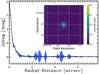
We searched for close visual companions of TOI-1444 with Adaptive Optics (AO) imaging. Close visual companions can bias the measured radius of a planet, or even be the source of false positives if the companion is itself an eclipsing binary. Data were collected on UT Dec 04 2019 with Gemini/NIRI (Hodapp et al., 2003). We collected 9 frames each with exposure time 8.2s in the Br $\gamma$ filter, and dithered the frame between each image by $\sim$ 1.3” in a grid pattern. The dithered science frames themselves are median combined to create a sky background frame. We reduced the data using a custom IDL code, which removes bad pixels, corrects for the sky background, flat-fields the data, and aligns and co-adds the individual images. We searched for companions by eye, and did not identify any additional sources within the field of view, which extends to at least 8” from the star in all directions. To assess the sensitivity of these images to companions, we injected several faint, fake companions into the data and scaled their brightness such that they would be detected at 5 $\sigma$ . The 5 $\sigma$ sensitivity is shown in Fig. 1 as a function of radius, along with a thumbnail image of the target.

Refer to caption — Figure 1: The contrast curve as function of radial separation from TOI-1444 using the AO Imaging from Gemini-NIRI. The inset is the image of target star.

4 Photometry

The TESS (Ricker et al., 2014) mission observed TOI-1444 in Sectors 15, 16, 17, 18, 19, 22, 24, 25 and 26 from UT Aug 15 2019 to July 04 2020. We downloaded the PDC_SAP light curves (Stumpe et al., 2012, 2014) of all sectors from the Mikulski Archive for Space Telescopes website²²2https://archive.stsci.edu. We removed all data points with a non-zero Quality Flag i.e. those suffering from cosmic rays or other known systematic issues.

4.1 Stellar Rotation Period

The TESS team reported one object of interest TOI-1444.01 with an orbital period of 0.47 day. Beginning with the transit parameters reported on the ExoFOP website³³3https://exofop.ipac.caltech.edu., we removed the data points taken within the transit window of TOI-1444.01. Using the resultant, out-of-transit light curve, we tried to measure the stellar rotation period of TOI-1444 using both Lomb-Scargle periodogram (Lomb, 1976; Scargle, 1982) and auto-correlation function (ACF, McQuillan et al., 2014). These two methods basically look for any quasi-periodic flux modulations that may be attributed to stellar rotation coupled with surface magnetic activity. Neither the periodogram nor the ACF detected a signal above 1% False Positive rate. Moreover, the highest peaks reported by these two methods did not agree. Therefore we could not measure the rotation period of the host from the flux variation seen in TESS light curve. The weak flux variation (standard deviation of about 1200 ppm for 2-min cadence over 300-day baseline) may be the result of a slow rotation and/or low stellar activity. Rotational broadening of TOI-1444 was not detectable in our spectrum above other broadening effects. Following Petigura (2015) we place an upper limit of $v~{}\text{sin}~{}i~{}<2$ km s^-1. The proxy for chromospheric activity in the Ca II H&K lines $S_{HK}$ is $0.145\pm 0.004$ . This is slightly lower than the median $S_{HK}$ of stars of similar B-V color ( 0.146, Isaacson & Fischer, 2010).

4.2 Search for Additional Transiting Planets

TOI-1444b was initially detected by the TESS Science Processing Operations Center (SPOC, Jenkins et al., 2016) in a transit search of Sectors 15 and 16 that occurred. The 0.47-day signal was detected at a 7.6 $\sigma$ level with an adaptive, noise-compensating matched filter (Jenkins et al., 2010); passed all the diagnostic tests performed and published in the resulting Data Validation reports. The vetting included tests for eclipsing binaries, such as an odd and even depth variation test, a secondary eclipse test, and a ghost diagnostic test. The difference imaging centroid test showed that the source of the transit signature was consistent with the target star TIC 258514800, but could not exclude nearby stars in the TIC catalog. The signal strength grew as additional observations were collected by TESS, and the difference imaging centroid test located the source within 3.6” once the full set of observations were completed in Sector 26.

We searched the TESS light curve for any additional transit signals particularly that around the 16-day periodicity of the candidate planetary signal seen in the radial velocity dataset (Section 5). We first removed the data points within the transit window of TOI-1444.01. We then fitted a cubic spline of length 1.5 days to detrend any long-term stellar or instrumental flux variation. We applied the Box-Least-Squares algorithm (BLS, Kovács et al., 2002) to the resultant light curve. Our BLS pipeline is implemented in C++ and has yielded a number of planet discoveries including other ultra-short-period planets e.g. K2-131b (Dai et al., 2017) and K2-141b (Barragán et al., 2018). We followed the suggested improvement of BLS as outlined in Ofir (2014). This involves using a nonlinear frequency grid given the theoretical scaling of transit duration with orbital period for stars of a certain mean density. We also adopted the signal detection efficiency (SDE) defined in Ofir (2014) to quantify the significance of a BLS signal. In short, SDE is the local variation of the BLS spectrum normalized by the local standard deviation. This helps to remove any period-related systematics.

We recovered TOI-1444.01 with a SDE =21. However, we did not detect any additional transiting signal with a SDE larger than 5. Visual inspection of the phase-folded light curve shows that none of the top candidate signals has a transit-like shape. We also did not detect any convincing single-transit events visually. Notably, there is no transiting signal consistent with the 16-day orbital period of the candidate planetary signal in the RV dataset. No additional transiting signal was found by the SPOC pipeline either.

4.3 Transit Modeling

We modeled the transit light curve of TOI-1444.01 or TOI-1444b to constrain its transit parameters. We started from the transit ephemeris reported by the TESS team. We used the Python package Batman (Kreidberg, 2015) to generate the model transit light curves. We also imposed a prior on the host star mean density using the result in Table 1. This precise prior on mean stellar density helps to break some of the degeneracy in modeling transit morphology and often lead to improved transit parameters (Seager & Mallén-Ornelas, 2003). We adopted a quadratic limb darkening profile. We imposed Gaussian priors (width of 0.3) on the limb-darkening coefficients $u_{1}$ and $u_{2}$ . We queried the EXOFAST⁴⁴4astroutils.astronomy.ohio-state.edu/exofast/limbdark.shtml. (Eastman et al., 2013) for the theoretical limb darkening given the spectroscopic parameters of TOI-1444 ( $u_{1}$ = 0.48, $u_{2}$ = 0.22). We also adopted the efficient sampling reparameterization of limb darkening coefficients proposed by Kipping (2013). The other parameters in our transit model are the orbital period $P_{\text{orb}}$ , the time of conjunction $T_{\text{c}}$ , the planet-to-star radius ratio $R_{\text{p}}/R_{\star}$ , the scaled orbital distance $a/R_{\star}$ and the impact parameter $b\equiv a\cos i/R_{\star}$ .

We first fitted all transits of TOI-1444b globally. We found the best-fit solution using the Levenberg-Marquardt method specifically using that implemented in Python package lmfit. Using this global fit as a template, we then fitted each individual transit allowing the mid-transit time to vary freely. The resultant transit times do not show quasi-sinusoidal variation as one would expect in the case of transit-timing variations. We did not detect any prominent periodicity; instead it is consistent with a linear ephemeris which we assume in subsequent analysis.

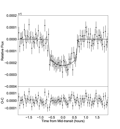
We sampled the posterior distribution of transit parameters with the affine-invariant Markov Chain Monte Carlo method as implemented in Python package emcee (Foreman-Mackey et al., 2013). We used 128 walkers starting from the maximum likelihood solution found by lmfit. With 50000 links, the Gelman-Rubin potential scale reduction factor reduced to below 1.01 suggesting convergence of the sampling process. We summarize the resultant posterior distribution in Table 2. Fig. 2 shows the phase-folded and binned TESS light curve and the best-fit transit model.

4.4 Phase Curve and Secondary Eclipse

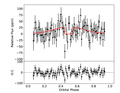
We looked for any phase curve variation and secondary eclipse of TOI-1444b in the TESS band. Again we removed data taken within the transit window of TOI-1444b. We then detrended any long-term stellar variation or systematic effect using the procedure outlined in Sanchis-Ojeda et al. (2013a). In short, a linear function in time whose width is at least one orbital period is fitted to remove local flux variation longer than the orbital period. In practice, we tried 1 $\times$ , 2 $\times$ or 3 $\times P_{\rm orb}$ , and found nearly identical results. We also compared PDC_SAP and SAP versions of TESS photometry; and found no substantial difference. Fig. 3 shows the phase curve variation from all TESS sectors of PDC_SAP photometry.

We then modeled the phase curve variation and secondary eclipse simultaneously. We modeled the secondary eclipse using Batman. We fixed the transit parameters using the best-fit primary transit solution and changed the limb darkening coefficients to 0. The phase curve variation was modeled as a Lambertian disk (e.g. Demory et al., 2016). The parameters in this model include the depth of secondary eclipse $\delta_{\rm sec}$ , the amplitude of illumination effect $A_{\rm ill}$ , the time of secondary eclipse $t_{\rm sec}$ and the phase offset of the illumination effect $\theta_{\rm ill}$ . To constrain the posterior distribution, we similarly ran an MCMC analysis with emcee (Foreman-Mackey et al., 2013). We found that both $\delta_{\rm sec}=27\pm 12$ ppm and $A_{\rm ill}=24\pm 10$ ppm showed marginal detection of no more than 2.5 $\sigma$ . The fact that $\delta_{\rm sec}$ are similar to $A_{\rm ill}$ in amplitude even though they are fitted separately boosts our confidence in these detections. $t_{\rm sec}$ centers around the half-way from mid-transit although with substantial errorbar $t_{\rm sec}=0.236\pm 0.019$ day or 0.502 $\pm 0.040$ in orbital phase. Again this is expected given the very short tidal circularization timescale of a planet on such a short-period orbit. The phase curve offset $\theta_{\rm ill}=16\pm 27^{\circ}$ shows a very weak preference for an eastward offset.

The TESS passband (600-1000 nm) extends substantially into the infrared that one may expect to see thermal emission from the planet as well as reflected star light. However, with only one band, we could not break the degeneracy between reflected stellar light and thermal emission from the planet. Fig. 4 captures this degeneracy in the Bond Albedo versus TESS band Geometric Albedo plane. The blue-shaded region shows the 68% confidence interval. Given how wide the confidence interval is, we refrain from making a strong interpretation of the marginal 2.5 $\sigma$ phase curve detection in TESS band. Phase curve observation in the infrared would consolidate the phase curve variation and may reveal the surface properties of TOI-1444b.

4.5 Ground-based Follow-up

We observed TOI-1444 on May 02 2020 during the transit window of planet b as predicted by the SPOC pipeline analysis of TESS Sectors 15 and 16. The observation was carried out in the Pan-STARSS $z$ -short band from the Las Cumbres Observatory Global Telescope (LCOGT; Brown et al., 2013) 1.0 m network node at the McDonald Observatory. The 4096x4096 LCO SINISTRO cameras have an image scale of $0\farcs 389$ per pixel, providing a field of view of $26\arcmin\times 26\arcmin$ . The standard LCOGT BANZAI pipeline (McCully et al., 2018) was used to calibrate the images, and the photometric data were extracted with the AstroImage (AIJ) software package Collins et al. (2017).

Since the $\sim 200$ ppm event detected by the SPOC pipeline is generally too shallow to detect with ground-based observations, we checked for a faint nearby eclipsing binary (NEB) that could be contaminating the SPOC photometric aperture. To account for possible contamination from the wings of neighboring star PSFs, we searched for NEBs at the positions of Gaia DR2 stars out to $2\farcm 5$ from the target star. If fully blended in the SPOC aperture, a neighboring star that is fainter than the target star by 9.3 magnitudes in TESS-band could produce the SPOC-reported flux deficit at mid-transit (assuming a 100% eclipse). To account for possible delta-magnitude differences between TESS-band and Pan-STARSS $z$ -short band, we included an extra 0.5 magnitudes fainter (down to TESS-band magnitude 20.0). We visually compared the light curves of the 85 nearby stars that meet our search criteria with models that indicate the timing and depth needed to produce the $\sim 200$ ppm event in the SPOC photometric aperture. We found no evidence of an NEB that might be responsible for the SPOC detection. By a process of elimination, we conclude that the transit is likely occurring on TOI-1444.

5 Radial Velocity Analysis

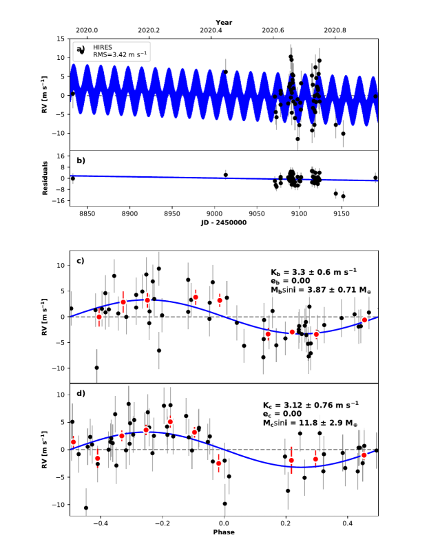
We obtained 59 high-resolution spectra of TOI-1444 from UTC Dec 15 2019 to Dec 25 2020 on the High Resolution Echelle Spectrometer on the 10m Keck I telescope (Keck/HIRES Vogt et al., 1994). Two of these are iodine-free spectra which serve as the template for radial velocity extraction. The rest were obtained with the iodine-cell in the light path to serve as the source for wavelength calibration and the reference for the line spread function. Each exposure of TOI-1444 was about 15 min achieving a median SNR of 140 per reduced pixel near 5500 Å. Whenever possible, we tried to obtain multiple exposures within each night; this helps to separate the radial velocity variation due to the short-period planet b from any longer-period stellar activity contamination. Such a strategy has been employed in the RV follow-up of many USP planets (e.g. Howard et al., 2013a). The radial velocity variation was extracted using the forward-modeling Doppler pipeline described in Howard et al. (2010). To quantify the stellar activity of TOI-1444, we analyzed the Ca II H&K lines and extracted the $S_{\rm HK}$ using the method of Isaacson & Fischer (2010). We looked for any correlation between the measured RV and activity index $S_{\rm HK}$ . We applied a Pearson correlation test which reported a $p$ -values of 0.65 i.e. a lack of correlation between the measured RV and $S_{\rm HK}$ . This again testifies the low activity of TOI-1444. The extracted RV and stellar activity indices are presented in Table 4.

5.1 Non-transiting planet c?

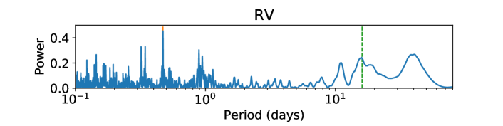
We first applied the Python package RVSearch ⁵⁵5https://github.com/California-Planet-Search/rvsearch to determine the number of planetary signals in our RV dataset. In short, RVSearch sequentially look for peaks in the LS periodogram of the RV dataset after removing the best-fit Keplerian model of planetary signals detected in previous iterations. The code stops when the Bayesian Information Criterion ( $\Delta$ BIC) no longer favors the addition of another planetary signal. RVSearch has been widely tested on known planetary systems. For more detail on RVSearch, we refer interested readers to Rosenthal et al (2021).

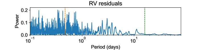
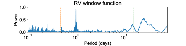
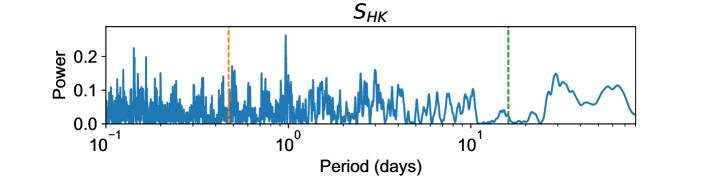
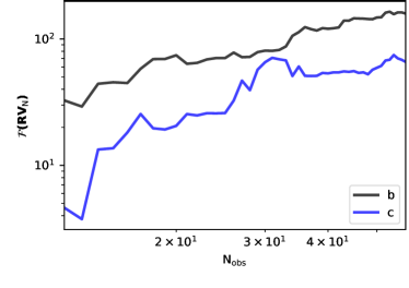
Applying RVSearch to TOI-1444, a strong peak at the transiting period of TOI-1444b is recovered (Fig.5). RVSearch detects a candidate 16-day signal. No corresponding peak is seen in the RV window function or the activity index $S_{HK}$ . Moreover, the strength of the 16-day periodicity steadily increased as we included more and more RV data in the periodogram. In contrast, a signal caused by stellar activity loses coherence over time because the underlying surface magnetic activity typically emerge and subside on weeks-to-months timescale for solar-like stars.

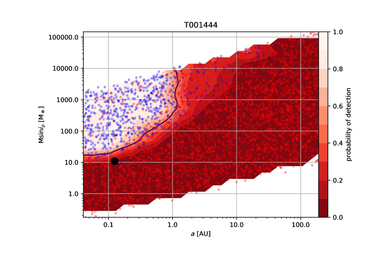
RVSearch can also perform injection and recovery test of planetary signals in the $M_{p}$ sin $i$ - $P_{\rm orb}$ plane. The result is a completeness contour showing the sensitivity of the RV dataset at hand to planetary signals of different strength and periodicity in addtion to the detected planets (e.g. Fig. 7). Given the current HIRES RV dataset for TOI-1444, we were unable to identify a third planetary signal. The completeness contour for that third planet is shown in Fig. 7. With the current HIRES dataset, other sub-Neptune planets (<10 $M_{\oplus}$ ) within 1AU of TOI-1444 can easily remain hidden from detection.

5.2 RadVel Model

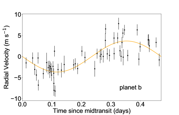
We first modeled the RV dataset using Keplerian models. We used the publicly available Python package RadVel (Fulton et al., 2018). Each planetary signal is described by its orbital period $P_{\rm orb}$ , time of inferior conjunction $T_{c}$ , eccentricity $e$ , argument of periastron $\omega$ and the RV semi-amplitude $K$ . We allowed an RV offset $\gamma$ , a linear RV trend $\dot{\gamma}$ and we included a jitter term to encapsulate any additional astrophysical or instrumental noise. We reparameterized $e$ and $\omega$ into $\sqrt{e}$ cos $\omega$ , $\sqrt{e}$ sin $\omega$ . Since the ephemeris is much better constrained with the transit data, we imposed Gaussian priors on $P_{\rm orb}$ and $T_{c}$ using the results from Section 4.3. We imposed uniform priors on the RV semi-amplitude $K$ , the jitter $\sigma_{\text{jit}}$ , $\sqrt{e}$ cos $\omega$ (with range [-1,1]), $\sqrt{e}$ sin $\omega$ ([-1,1]), $\gamma$ and $\dot{\gamma}$ . Our likelihood function is as follows:

\mathcal{L}=\prod_{i}\left({\frac{1}{\sqrt{2\pi(\sigma_{i}^{2}+\sigma_{\text{jit}}^{2})}}}\exp\left[-\frac{[RV(t_{i})-\mathcal{M}(t_{i})]^{2}}{2(\sigma_{i}^{2}+\sigma_{\text{jit}}^{2})}\right]\right)

(1)

where $RV(t_{i})$ is measured RV; $\mathcal{M}(t_{i})$ is the sum of Keplerian planetary signals, a constant RV offset $\gamma$ and a linear RV trend $\dot{\gamma}t_{i}$ ; $\sigma_{i}$ is the internal uncertainty.

We varied the number of planets in our model; and we tested if the current dataset supports non-zero eccentricity and $\dot{\gamma}$ . We selected the best model using both Bayesian Information Criterion ( $\Delta$ BIC) and Akaike information criterion ( $\Delta$ AIC). Our best-fit model (lowest $BIC$ and $AIC$ ) contains the RV signals of planet b and a non-transiting planet with a 16-day orbit identified by RVSearch. Non-zero eccentricity for either planet was not preferred by the current dataset. A linear RV trend of $\dot{\gamma}=-0.008\pm 0.012$ m s^-1 is marginally disfavored by the current dataset with $\Delta BIC\approx-2$ . We then performed an MCMC analysis to sample to posterior distribution of the various parameters. The sampling procedure is similar to that descrbied in Section 4.3. We summarize the posterior distribution in Table 2.

5.3 Gaussian Process Model

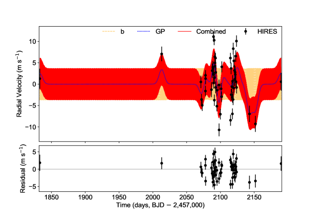
The RV residuals after removing the best 2-planet Keplerian model still shows a root-mean-square variation (RMS) of 3.4 m s^-1 which is substantially larger than the internal uncertainties in Table 4. Moreover, the RV residuals visually display some correlated noise component in Fig. 8. We investigated if these residual noises can be tidied up by a Gaussian Process (GP) model (e.g. Haywood et al., 2014; Grunblatt et al., 2015) and and disentangle the planetary signal from the stellar activityf.

We adopted the GP model used in our previous works (Dai et al., 2017, 2019). Stellar surface magnetic activity rotating in and out of view of the observer is chiefly responsible for the correlated stellar noise in RV measurements, the quasi-sinusoidal flux variation in the light curve and the variation of chromospheric activity index $S_{HK}$ (e.g., Aigrain et al., 2012). In other words, these effects stem from the same underlying physical process, we model them with a common GP model. The plan of attack is to train a quasi-periodic GP model on the out-of-transit TESS light curves and the HIRES $S_{HK}$ index, before applying it the RV dataset. Our kernel has the following form:

C_{i,j}=h^{2}\exp{\left[-\frac{(t_{i}-t_{j})^{2}}{2\tau^{2}}-\Gamma\sin^{2}{\frac{\pi(t_{i}-t_{j})}{T}}\right]}+\left[\sigma_{i}^{2}+\sigma_{\text{jit}}^{2}\right]\delta_{i,j}

(2)

where $C_{i,j}$ represents the covariance matrix; $\delta_{i,j}$ is the Kronecker delta function; $h$ is the covariance amplitude; $t_{i}$ is the time of $i$ th observation; $\tau$ is the correlation timescale; $\Gamma$ is the relative importance between the squared exponential and periodic parts of the kernel; and $T$ is the period of the covariance; $\sigma_{i}$ is the reported uncertainty and $\sigma_{jit}$ is a jitter term. Our likelihood function is as follows:

\log{\mathcal{L}}=-\frac{N}{2}\log{2\pi}-\frac{1}{2}\log{|\bf{C}|}-\frac{1}{2}\bf{r}^{\text{T}}\bf{C}^{-\text{1}}\bf{r}

(3)

where $\mathcal{L}$ is the likelihood function; $N$ is total number of RV data points; $\bf{C}$ represents the covariance matrix; and $\bf{r}$ is the residual the observed RV minus the model RV.

We ran an MCMC analysis (similar to that described in Section 4.3) on the TESS light curves to constrain the posterior distribution of the various hyperparameters. As we mentioned earlier, we could not robustly detect the stellar rotation period in the TESS light curve from a periodogram analysis. This is may be due to the low activity of the host star. Correspondingly, our GP model of the TESS photometry yielded very broad posterior distribution on various hyperparameters. We then tried if the addition of HIRES $S_{HK}$ index gave better constraints on the hyperparameters. $S_{HK}$ was sparsely sampled and only varied very mildly with RMS of about 0.004. Consequently, $S_{HK}$ did not significantly improve the constraints on the GP hyperparameters.

Therefore, we chose to let the hyperparameters float freely in our final GP analysis of the RV dataset. The exception is that we did limit $T$ the covariance period (a proxy for stellar rotation period) between 1 and 200 days to avoid inference with the 0.47-day planet b. Understandably, without an imposed prior on the various hyperparameters, the flexibility of this GP model subsumed the signal of the candidate 16-day planet c. Planet c only has an upper limit $K_{c}<4.3$ m s^-1 at 95% confidence level in our GP model. In fact, the lowest BIC GP model only included the signal from planet b (Fig. 9). An MCMC analysis showed that the posterior distribution of the semi-amplitude of planet b is $K_{b}=3.59\pm 0.75$ m s^-1 which agrees with the $K_{b}=3.30^{+0.58}_{-0.59}$ m s^-1 found by RadVel. Since the GP model has far more complexity than the RadVel model and the $K$ value came out less well constrained, we adopted the results from RadVel for further analyses in this work.

Table 2: Planetary Parameters of TOI-1444

Parameter	Symbol	Posterior Distribution
Planet b
Planet/Star Radius Ratio	$R_{p}/R_{\star}$	$0.01410^{+0.00060}_{-0.00058}$
Time of Conjunction (BJD-2457000)	$t_{c}$	$1711.3676\pm 0.0016$
Impact Parameter	$b$	$0.38\pm 0.14$
Scaled Semi-major Axis	$a/R_{\star}$	$2.73^{+0.078}_{-0.074}$
Orbital Inclination (deg)	$i$	$82^{+3}_{-2}$
Orbital Eccentricity	$e$	0 (fixed)
Orbital Period (days)	$P_{\rm orb}$	$0.4702694\pm 0.0000044$
Semi-amplitude (m/s)	$K$	$3.30^{+0.58}_{-0.59}$
Planetary Radius ( $R_{\oplus}$ )	$R_{\rm p}$	1.397 $\pm 0.064$
Planetary Mass ( $M_{\oplus}$ )	$M_{\rm p}$	3.87 $\pm 0.71$
Secondary Eclipse Depth (ppm)	$\delta_{\rm sec}$	$27\pm 12$
Time of Secondary Eclipse (days)	$t_{\rm sec}$	$0.236\pm 0.019$
Amplitude of Illumination Effect (ppm)	$A_{\rm ill}$	$24\pm 10$
Phase Offset of Illumination Effect (^∘)	$\theta_{\rm ill}$	$16\pm 27$
Planet c
Time of Conjunction (BJD-2457000)	$t_{c}$	$713.0\pm 2.0$
Orbital Period (days)	$P_{\rm orb}$	$16.066\pm 0.024$
Orbital Eccentricity	$e$	0 (fixed)
Semi-amplitude (m s^-1)	$K$	$3.12^{+0.75}_{-0.76}$
Projected Planetary Mass ( $M_{\oplus}$ )	$M_{\rm p}\sin i$	11.8 $\pm$ 2.9
RV Jitter (m s^-1)	$\sigma$	$3.2\pm 0.4$

6 Discussion

6.1 Are the known USPs still predominantly rocky?

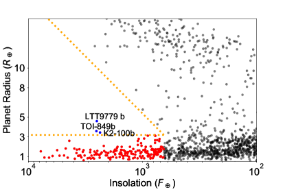
Before any discussion, we would like to loosely define USPs as terrestrial planets ( $<2R_{\oplus}$ ) with orbital period less than one day (the prevailing definition in the literature) as well as those with an insolation level larger than 650 $F_{\oplus}$ (see Table 3 for the complete list). 650 $F_{\oplus}$ is an empirical boundary, identified by Lundkvist et al. (2016); Sanchis-Ojeda et al. (2014), beyond which photoevaporation is so strong that any Neptune-sized planets are quickly stripped down to their rocky cores by the strong stellar irradiation (Fig. 10), thereby creating a “Hot Neptune Desert”.

Dai et al. (2019) performed a uniform analysis of all transiting USPs that also have RV mass constraints. In particular, they used Gaia parallax information to better constrain the host stellar properties. The increased precision on stellar radius translated to increased precision on planetary radii. Moreover, the mean stellar density from Gaia and spectroscopy further disentangled degeneracies in transit modeling. The results significantly improved constraints on planetary radii. For example, the radius constraint of Kepler-78 b improved from $R_{p}=1.20\pm 0.09R_{\oplus}$ in Howard et al. (2013b) to $R_{p}=1.228^{+0.018}_{-0.019}R_{\oplus}$ with Gaia. Dai et al. (2019) also applied a Gaussian Process model uniformly to all USP planets that required mitigation of stellar activity contamination in RV datasets. The improved mass and radius constraints on the sample of 10 USPs revealed a prevalence of 35%Fe-65%MgSiO₃ Earth-like composition.

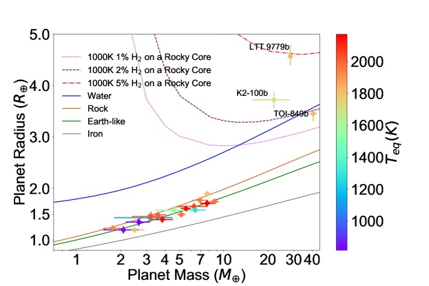
In this work, we applied the same set of analysis to TOI-1444b and interpret the resultant mass and radius constraint along with other USP planets. The interest in USP planets has boomed in recent years, the number of USP RV mass measurements increased from 10 in Dai et al. (2019) to 17 at the time of writing of this work. Moreover, the inclusion of Gaia parallax information and Gaussian Process modeling has become a standard practice in these new USP papers (Table 3). This puts the new USPs reported by different groups on relatively equal footing and ready for comparison. In Fig. 11 upper panel, we show the mass and radius of all USP planets with RV mass measurements. At a glance, USPs seem to cluster around an Earth-like composition. To quantify the compositions, we adopted a simple two-layer model where planets have an iron core and a MgSiO₃ mantle. We used the procedure described by Zeng et al. (2016) to convert the measured mass and radius of the planet to a Fe-MgSiO₃ ratio. For an individual planet, the confidence interval is relatively wide e.g. TOI-1444b can have 43 $\pm$ 30% of its mass in iron given our mass and radius measurement. However, as an ensemble, the USP planets generally cluster around the Earth-like composition with a weighted mean of 32 $\pm 4\%$ mass in an iron core. This is consistent with the general picture that planets at the lower peak of the bimodal radius distribution are predominantly rocky (Rogers, 2015; Dressing et al., 2015; Fulton et al., 2017).

We note that we have excluded two USPs from the averaging of iron core mass fraction. The mass of TOI-561 reported by Weiss et al. (2021) and Lacedelli et al. (2021) differ by almost a factor of two. More RV data are being taken to resolve this discrepancy (Brinkman et al, in prep). By focusing on the USP planets i.e. planets that are most strongly irradidated, we hope to probe the exposed planetary cores directly without worrying about the degeneracy introduced by a planetary atmosphere. This assumption has held up well for most USPs in our sample. We examined the composition of USP against the insolation level. If a substantial atmosphere were present on an USP, one may expect the scale height to vary strongly with insolation level. The scale height variation would have translated to a correlation between insolation level and the inferred planetary composition. However no correlation between insolation and iron core mass fraction was found (Fig. 11). That said, we did exclude 55 Cnc e, one of the largest and coolest USPs, from our analysis. The strong phase offset seen in Spitzer observation of 55 Cnc e (Demory et al., 2016) demands a strong heat circulation between the day and the night side of the planet that, as Angelo & Hu (2017) argue, requires the presence of an atmosphere on 55 Cnc e. The larger planet mass and the cooler equilibrium temperature of 55 Cnc e may help retain its atmosphere compared to other USPs in the current sample.

6.2 USP versus Ultra-hot Neptunes

What is the relation between the USP planets and the recently reported ultra-hot Neptunes K2-100 b (Mann et al., 2017), LTT 9779 b (Jenkins et al., 2020), TOI-849 b(Armstrong et al., 2020)? Are they the same group of planets that only differ in size? In this section, we will show that USPs and ultra-hot Neptunes differ in planetary/stellar properties and system architecture suggesting that they are probably two distinct groups of planets.

We identified a sample of three very hot Neptunes between 3-5 $R_{\oplus}$ and with an insolation level $>2000F_{\oplus}$ (Fig. 10). Again $>650F_{\oplus}$ is the empirical boundary of “Hot Neptune Desert” proposed by Lundkvist et al. (2016). $>2000F_{\oplus}$ securely put these planets within the “Desert”. Currently, there are three confirmed hot Neptunes straggling in this so-called "Hot Neptune Desert": LTT 9779 b(Jenkins et al., 2020), TOI-849 b(Armstrong et al., 2020), and K2-100b (Mann et al., 2017) that have well-measured mass and radius. We put these hot Neptunes in the same mass radius diagram with the USP planets (Fig. 11 lower panel). Clearly, the USPs and the hot Neptunes occupy different part of the mass-radius parameter space. The USPs are all below 10 $M_{\oplus}$ , even though RV mass measurements bias towards the detection of heavier planets (a point we will return to later). The USPs also cluster around an Earth-like composition of iron-rock mixture. However, the three close-in hot Neptunes are near or above 100% water composition line in the mass radius diagram. This indicates the presence of a substantial H/He atmosphere or a water envelope for these planets. If we assume that they have Earth-like rocky cores, a 1-5% mass fraction H/He envelope is needed to reproduce the observed mass and radius. Recent Spitzer phase curve and secondary eclipse observations of LTT 9779 b pointed to the presence of a heavy-molecular weight (e.g. CO) atmosphere (Crossfield et al., 2020; Dragomir et al., 2020).

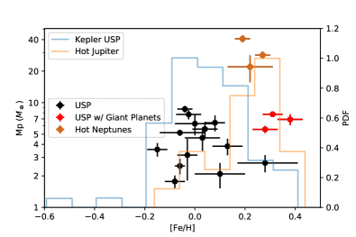
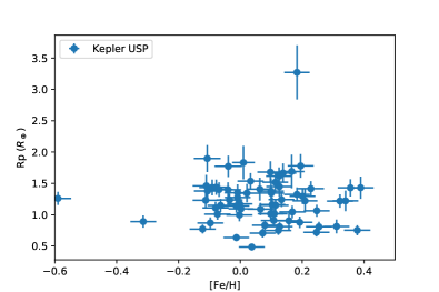
Winn et al. (2017) showed that the metallicity of USP host stars are solar-like which is similar to the longer-period sub-Neptune planets commonly discovered by Kepler (blue histogram in Fig. 12). On the other hand, hot Jupiters are known to preferentially occur around metal-rich systems (orange histogram in Fig. 12). Interestingly, the three hottest Neptunes all have similarly metal-rich host stars: LTT 9779 with [Fe/H] = 0.27 $\pm 0.03$ (Jenkins et al., 2020); K2-100 with [Fe/H] = 0.22 $\pm 0.09$ (Mann et al., 2017); TOI-849 with [Fe/H] = 0.19 $\pm 0.03$ (Armstrong et al., 2020). Even though the sample size is only 3, the distribution of hot Neptunes is beginning to show a stark distinction from the solar-like distribution of USP, and bears more resemblance to the metal-rich environments of hot Jupiters. This result is reminiscent of the previous work by Dong et al. (2018) who showed an even more statistically robust preference for hot Neptunes to occur around metal-rich host stars if we consider orbital periods as long as 10 days.

Another feature that differentiates USPs from hot Neptunes is the presence of additional planetary companions. 14 out of the 17 well-characterized USPs have other planetary companions in the same system discovered by transits or radial velocity follow-up (Table 3). We further note that the RV datasets of the three systems where the USPs remain the only detected planet (K2-131, Kepler-78 and K2-291) are heavily contaminated by activity-induced RV variation that amounts to tens of m s^-1. We applied RVSearch to these systems to constrain the sensitivity of the existing RV dataset to additional planetary signals (similar to Fig. 7). RVSearch showed that the activity-induced RV variation could easily inhibit the detection of injected planetary signals with < $15M_{\oplus}$ within 1 AU. Turning our attention to the hot Neptunes, among the three hottest Neptunes, none of them have detected additional planets even though some of RV monitoring baselines extended more than 100 days (Table 3). This hints that hot Neptunes tend to be “lonely” similar to the hot Jupiters.

To sum up, USPs planets tend to be rocky in composition while hot Neptunes possess substantial H/He atmospheres or other volatile envelopes. USPs occur in stars with solar-like abundances, while hot Neptunes are preferentially found in metal-rich systems. USPs tend to have other close-in planetary companions while hot Neptunes tend to be lonely. These properties distinguish the two groups. Moreover, the properties of the hottest Neptunes are quite similar to their bigger cousins hot Jupiters. This similarity actually extends to many Neptune-sized planets between 2-6 $R_{\oplus}$ and orbital periods of 1-10 days as pointed out by Dong et al. (2018). Finally, we close the section by noting that USPs, hot Jupiters and <10-day hot Neptunes all occur at about 1% level around sun-like stars (e.g. Sanchis-Ojeda et al., 2014; Cumming et al., 2008; Dong et al., 2018). However, the hot Neptunes on sub-day orbits seem rarer. The Kepler USPs from Sanchis-Ojeda et al. (2014) represent a uniformly studied sample amenable to occurrence rate studies. Among the 67 confirmed/validated USP candidates only 1 (KOI-3913) has a radius in the Neptune regime >3 $R_{\oplus}$ . The rest are all below 2 $R_{\oplus}$ (Fig. 12). Even though this is still small number statistics, the Kepler USP sample suggests that hot Neptunes on sub-day orbit are probably as rare as 0.1-0.01% level around sun-like star. Future TESS occurrence rate studies will firm up this number. Another system worth mentioning is NGTS-4b (West et al., 2018) a 3.2 $R_{\oplus}$ hot Neptune on a 1.3-day orbit around a K star. It is less strongly irradiated compared to K2-100b, TOI-849 b and LTT 9779 b, right on the edge of the “hot Neptune Desert”. It shows many similarities with K2-100b, TOI-849 b and LTT 9779 b: likely enshrouded by an atmosphere, having no other planetary companions. However, the metallicity of its host star was reported to be surprisingly low: reported in units of total metal [M/H] = -0.28 $\pm 0.10$ . We encourage future observation to confirm the reported low metallicity.

Table 3: Additional planetary companions in USP and hot-Neptune systems ranked by planet mass

System	Additional Planets Detected?	Comments	Reference
Kepler-78	N	Activity-induced RV variation (50 m s^-1 peak to peak, 12.5-day periodicity) prevents detection of additional planets	Howard et al. (2013a)
GJ 1252	Y	15 m/s drift over 10 days likely due to an additional planet	Shporer et al. (2020)
K2-229	Y	2 additional transiting planets on 8 and 31-day orbit	Santerne et al. (2018)
LTT 3780	Y	1 additional transiting planet on 12-day orbit	Cloutier et al. (2020)
K2-36	Y	1 additional transiting planet on 5-day orbit	Damasso et al. (2019)
Kepler-10	Y	1 additional transiting planet on 45-day orbit	Dumusque et al. (2014)
TOI-1444	Y	1 additional non-transiting planet on 16-day orbit	This work
CoRoT-7	Y	1 additional non-transiting planet on 3.7-day orbit	Haywood et al. (2014)
K2-141	Y	1 additional non-transiting planet on 7-day orbit	Malavolta et al. (2018)
HD 3167	Y	1 additional non-transiting planet on 8.5-day orbit and 1 transiting planet on 29-day orbit	Christiansen et al. (2017)
HD 80653	Y	RV drift suggests one additional planet of 0.37 $\pm 0.08$ $M_{\rm Jup}$ (a $/$ AU)^-2	Frustagli et al. (2020)
K2-131	N	Activity-induced RV variation (60 m s^-1 peak to peak, 3-day periodicity) prevents detection of additional planets	Dai et al. (2017)
K2-291	N	Activity-induced RV variation (30 m s^-1 peak to peak, 19-day periodicity) prevents detection of additional planets	Kosiarek et al. (2019)
WASP-47	Y	2 additional transiting planets with a 4-day giant planet; 1 non-transiting giant planet on 600-day orbit	Vanderburg et al. (2017)
K2-106	Y	1 additional non-transiting planet on 13-day orbit	Guenther et al. (2017)
55 Cnc	Y	4 additional non-transiting planets between 14 and 5000 days including a close-in giant planet	Bourrier et al. (2018)
HD 213885	Y	1 additional non-transiting planet on 5-day orbit	Espinoza et al. (2020)
K2-100	N	Activity-induced RV variation (100 m s^-1 peak to peak, 4.3-day periodicity) prevents detection of additional planets	Barragán et al. (2019)
LTT 9779	N	20 days of RV baseline	Jenkins et al. (2020)
TOI-849	N	>400 days of RV baseline	Armstrong et al. (2020)

6.3 Implications for Planet Formation

The top contenders of USP formation theory invoke the secular interaction between USPs and longer-period planets (Petrovich et al., 2018; Pu & Lai, 2019). Consider a USP that formed initially on longer orbital periods 2-10 days range. This is beyond the dust sublimation radius and where many Kepler planets are found today. If there are other planets in the same system with enough angular momentum deficit (AMD) i.e. the angular momentum difference between a system with coplanar, circular orbits and a systems with eccentric, mutually inclined orbits, secular interaction between the planets could shuffle the AMD around. Since the progenitors of USPs are the innermost planet of their system, they have the lowest angular moment per unit mass. The same AMD could thus induce a significantly eccentric and inclined orbit. The augmented tidal interaction with the host star at periastron could then shrink the orbit of the USPs. This secular scenario has gained observational support as the USPs are indeed observed on more inclined orbits compared to other Kepler planets and USPs often have a longer orbital period ratio relative to their neighbors—likely a consequence of orbital decay (Dai et al., 2018; Steffen & Coughlin, 2016). Here, we point out another observational support of the secular theory i.e. USP must have additional planets to initiate the secular interaction and provide enough AMD. In Table 3 we showed that USPs almost always have additional planetary companions (14/17). For 55 Cnc, the existing RV dataset is big enough to reveal orbital eccentricities of the various planets thereby allowing us to gauge whether the amount of AMD in a system could alter USP orbit significantly. Indeed, Hansen & Zink (2015) showed that the architecture of 55 Cnc does contain the requisite AMD and is in general consiten with the secular formation scenario. Future extensive RV follow-up of USPs may extend this AMD test to other systems.

Hot Neptunes, including those on sub-day orbits, show striking similarities with hot Jupiters: 1)they favor metal-rich environments; 2)they tend to be the only planet in a system; 3)their occurrence rate sums up to about 1% occurrence rate within 10-days around sun-like stars (Dong et al., 2018). Another similarity between hot Jupiters and hot Neptune is that many hot Neptunes were also observed to be on misaligned orbits characterized by large stellar obliquities e.g. Kepler-63 (Sanchis-Ojeda et al., 2013b), HAT-P-11 (Sanchis-Ojeda & Winn, 2011) and WASP-107 (Dai & Winn, 2017; Rubenzahl et al., 2021). For hot Jupiters, a large spin-orbit angle has traditionally been interpreted as a signpost of a dynamically hot formation scenario that tilted planet orbit while also triggering orbital decay ([see the view by Dawson & Johnson, 2018). The large obliquity of many hot Neptunes is suggestive of a formation channel similar to that of the hot Jupiters. It will be instructive to extend obliquity measurements to ultra-hot Neptunes such as K2-100, LTT 9779 and TOI-849, although this is technically challenging with current generation spectrographs. Berger et al. (2020) also presented evidence that hot Neptunes are preferentially found around evolved stars. This could be an indication that the hot Neptunes migrated as a result of host stellar evolution.

Two recent planet formation theoretical works may also shed light on the distinction between USPs and hot Neptunes. Adams et al. (2020) performed a simple analysis that optimized the total energy of a pair of forming planets assuming the conservation of angular momentum, constant total mass reservoir and fixed orbital spacings. They found that when the total available mass is low ( $\lesssim 40M_{\oplus}$ , a number that depends on stellar mass, semi-major axis etc), the energy-optimized state is an equal partition of mass between two competitively growing planets. This thus tends to create a multi-planet systems with intra-system uniformity that was seen in many observed sub-Neptune multi-planet systems (Millholland et al., 2017; Weiss et al., 2018; Wang, 2017). On the other hand, when the total mass is high enough, the system switches to a different optimized state in which the mass is concentrated in one of the planets, thereby creating a dominant, possibly lonely planet that may undergo runaway accretion. Whether a system does go into the runaway accretion state, as pointed out by Lee (2019) and Chachan et al. (2021), further depends on the local hydrodynamic flow conditions, the local opacity and the time of core emergence i.e. whether gas is still present in the disk. These theories put the USPs and hot Neptunes into perspective: in a metal-rich (high [Fe/H]) disk, the planetesimals assemble quickly and grow large enough to accrete the remaining gas in the disk (see also Dawson et al., 2015). If the total planetesimal mass is above some threshold, one particular planet embryo grow to be the dominant planet in a system as Adams et al. (2020) would predict. In short, metal-rich systems tend to breed hot Neptunes and hot Jupiters. On the other hand, the rocky USP planets could be the product of late assembly in gas-depleted disk in which core assemebly proceeds oligarchically and slowly. This explains why their occurrence does not correlate strongly with host star metallicity. Adams et al. (2020) would further predict that USP planets come in multi-planet systems where the planets are similar in size.

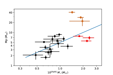
Table 3 shows that there are three USPs that also have detected giant planet companions. They are 55 Cnc with a 14.6-day giant planet (Butler et al., 1997); WASP-47 with with 4.2 and 600-day giant planets(Becker et al., 2015b; Neveu-VanMalle et al., 2016) and HD 80653 with a strong RV trend likely indicative of a giant planet 0.37 $\pm 0.08$ $M_{\rm Jup}$ (a $/$ AU)^-2 (Frustagli et al., 2020). The attentive reader might have already guessed that these three systems are also the most metal-rich among the USP sample with [Fe/H] = 0.31 $\pm 0.04$ , 0.38 $\pm$ 0.05 and 0.28 $\pm$ 0.05 respectively (red points in Fig. 12). These three USPs also happen to be the more massive ones among the USP sample (Fig. 12). One is tempted to ask: are USPs in metal-rich environments also the more massive ones? We use the $M_{\star}*10^{[Fe/H]}$ as a proxy for the surface density of solid material available to USP growth. Dai et al. (2020) applied a Minimum-mass Extrasolar Nebula framework to Kepler sub-Neptune planets which suggeested that the disk solid mass displayed a linear scaling with host star mass even within the innermost 1AU. $M_{\star}*10^{[Fe/H]}$ may be a reasonable proxy for the solid disk density. We found $M_{\star}*10^{[Fe/H]}$ and USP mass do show a positive correlation with a p-value of 0.04 in a Pearson test (Fig. 12). This correlation may suggest that the surface density of solids in the disk directly controls the overall availability of solids, the assembly rate, and eventually manifests as the size of planetary cores that emerge out of the disks.

6.4 Threshold for runaway accretion?

As we argued above, USPs are probably a distinct group compared to hot Jupiters and hot Neptunes given the differences in host star metallicity and planet architecture. USPs are most likely cores of planets that escaped runaway accretion in the first place i.e. superEarths or sub-Neptunes. The rate of atmospheric erosion particularly photoevaporation shows a steep dependence on planet mass. It is suppressed by orders of magnitude for giant planets (e.g. Murray-Clay et al., 2009). Briefly, this is because the gravitational potential well deepens with planet mass, but the heating efficiency of XUV irradiation does not. For example, the H/He envelopes on a $5\,M_{\oplus}$ planet can be easily stripped in 100 Myr at 0.1 AU around a G-type star, but the mass loss timescale quickly shoots up to more than a Hubble time for planetary cores with >10-15 $M_{\oplus}$ depending on the insolation the planet receives (Wang & Dai, 2019). In summary, planets heavier than Neptune can only lose a small fraction of their envelope over their lifetime; thus they are unlikely to be stripped down to a rocky core that is observed as a USP planet today.

Therefore, the sample of USP planets help to place an upper limit on the threshold of runaway accretion. RV follow-up observations are heavily biased towards the detection of more massive planets. However, this bias works in our favor as we are probing an upper limit in mass. If one assumes a radiative outer layer, the critical mass for runaway accretion only has a logarithmic dependence on the local disk properties (e.g. Rafikov, 2006). In other words, it is not sensitive to the location where the planets formed; and is estimated to be about $10\,M_{\oplus}$ (Rafikov, 2006). If one more carefully accounts for the envelope opacity, the threshold mass may be more variable between 2 and $8\,M_{\oplus}$ (Lee & Chiang, 2016). The lower the local gas opacity, the lower the mass threshold for run-away accretion (see also Chachan et al., 2021). In this framework, the super-puffs– low density, gas-rich planets with <5 $M_{\oplus}$ , >5 $R_{\oplus}$ , likely formed beyond the snowline where the opacity is low (e.g. Kepler-51 Libby-Roberts et al., 2020). Coming back to the current sample of 17 USPs, they are mostly consistent with exposed rocky cores. They seem to probe the upper limit of the threshold for run-away accretion. This seems to be at the predicted $8\,M_{\oplus}$ for the high-opacity inner disk ( $\sim$ 0.1 AU) where USPs have likely formed. We note that the only USP that is suspected to have some atmosphere is 55 Cnc e (Angelo & Hu, 2017) right at $\sim 8M_{\oplus}$ . This putative current-day atmosphere on 55 Cnc e was also suggested to be secondary in nature. 55 Cnc e was neither detected in Lyman- $\alpha$ (Ehrenreich et al., 2012) or metastable He (Zhang et al., 2021) transit observations.

7 Summary

In this work, we report the transiting USP TOI-1444b discovered in TESS photometry. We performed extensive follow-up of the system including AO imaging with Gemini/NIRI, Doppler monitoring with Keck/HIRES etc. These follow-up observations confirmed the planetary nature of the transiting signal and characterized the system. We also make use of this opportunity to analyze all USPs with precise mass and radius measurements and compare them with the recently reported ultra-hot Neptune planets. Our key findings are as follows:

•

TOI-1444b is a 0.47-day transiting USP with a radius of 1.397 $\pm 0.064R_{\oplus}$ and a mass of 3.87 $\pm 0.71M_{\oplus}$ consistent with a rocky composition.
•

We report a tentative 2.5 $\sigma$ detection of the phase curve variation and secondary eclipse of TOI-1444b in TESS band. Future observation of this target in 2 sectors during the TESS Extended Mission (S49 and S52) could help confirm this detection. However, observations at different wavelengths are needed to disentangle the thermal emission and reflected light contribution.
•

No additional transiting planets were found in the observed 9 sectors of TESS light curve. RV follow-up of Keck/HIRES revealed a non-transiting planet candidate on a 16-day orbit with a minimum mass of 11.8 $\pm 2.9M_{\oplus}$ .
•

USP planets and ultra-hot Neptunes are likely distinct groups of planets. Hot Neptunes preferentially occur around metal-rich systems, whereas USPs occur around stars with solar-like abundance. USPs are almost always found in multi-planet systems, whereas hot Neptunes tend to be “lonely”. USPs are exposed rocky cores that cluster around Earth-like composition. Hot Neptunes require H/He atmosphere or other volatile to explain their mass and radius. ultra-hot Neptunes are likely rarer than USPs by 1-2 orders of magnitude.
•

Metal-rich environments breed a diversity of planetary systems from USP, hot Neptunes to hot Jupiters (see also Petigura et al., 2013). USPs in systems with more solid materials tend to be more massive, although none of them are above the $8M_{\oplus}$ threshold for runaway accretion.

We thank Heather Knutson, Yayaati Chachan and Shreyas Vissapragada for insightful discussions. We thank the time assignment committees of the University of California, the California Institute of Technology, NASA, and the University of Hawaii for supporting the TESS-Keck Survey with observing time at Keck Observatory and on the Automated Planet Finder. We thank NASA for funding associated with our Key Strategic Mission Support project. We gratefully acknowledge the efforts and dedication of the Keck Observatory staff for support of HIRES and remote observing. We recognize and acknowledge the cultural role and reverence that the summit of Maunakea has within the indigenous Hawaiian community. We are deeply grateful to have the opportunity to conduct observations from this mountain. We thank Ken and Gloria Levy, who supported the construction of the Levy Spectrometer on the Automated Planet Finder. We thank the University of California and Google for supporting Lick Observatory and the UCO staff for their dedicated work scheduling and operating the telescopes of Lick Observatory. This paper is based on data collected by the TESS mission. Funding for the TESS mission is provided by the NASA Explorer Program. This work makes use of observations from the LCOGT network. LCOGT telescope time was granted by NOIRLab through the Mid-Scale Innovations Program (MSIP). MSIP is funded by NSF. Part of this work has been carried out within the framework of the National Centre of Competence in Research PlanetS supported by the Swiss National Science Foundation. ECM acknowledges the financial support of the SNSF. Based on observations obtained at the international Gemini Observatory, a program of NSF’s NOIRLab, which is managed by the Association of Universities for Research in Astronomy (AURA) under a cooperative agreement with the National Science Foundation. on behalf of the Gemini Observatory partnership: the National Science Foundation (United States), National Research Council (Canada), Agencia Nacional de Investigación y Desarrollo (Chile), Ministerio de Ciencia, Tecnología e Innovación (Argentina), Ministério da Ciência, Tecnologia, Inovações e Comunicações (Brazil), and Korea Astronomy and Space Science Institute (Republic of Korea). J.M.A.M. is supported by the National Science Foundation Graduate Research Fellowship Program under Grant No. DGE-1842400. J.M.A.M. acknowledges the LSSTC Data Science Fellowship Program, which is funded by LSSTC, NSF Cybertraining Grant No. 1829740, the Brinson Foundation, and the Moore Foundation; his participation in the program has benefited this work. D.H. acknowledges support from the Alfred P. Sloan Foundation, the National Aeronautics and Space Administration (80NSSC19K0379), and the National Science Foundation (AST-1717000). Resources supporting this work were provided by the NASA High-End Computing (HEC) Program through the NASA Advanced Supercomputing (NAS) Division at Ames Research Center for the production of the SPOC data products. We acknowledge the use of public TESS Alert data from pipelines at the TESS Science Office and at the TESS Science Processing Operations Center. JNW thanks the Heising-Simons foundation for support. D. D. acknowledges support from the TESS Guest Investigator Program grant 80NSSC19K1727 and NASA Exoplanet Research Program grant 18-2XRP18_2-0136.

References

Adams et al. (2016) Adams, E. R., Jackson, B., & Endl, M. 2016, AJ, 152, 47
Adams et al. (2020) Adams, F. C., Batygin, K., & Bloch, A. M. 2020, MNRAS, 494, 2289
Aigrain et al. (2012) Aigrain, S., Pont, F., & Zucker, S. 2012, MNRAS, 419, 3147
Angelo & Hu (2017) Angelo, I., & Hu, R. 2017, AJ, 154, 232
Armstrong et al. (2020) Armstrong, D. J., Lopez, T. A., Adibekyan, V., et al. 2020, Nature, 583, 39
Barragán et al. (2018) Barragán, O., Gandolfi, D., Dai, F., et al. 2018, A&A, 612, A95
Barragán et al. (2019) Barragán, O., Aigrain, S., Kubyshkina, D., et al. 2019, MNRAS, 490, 698
Becker et al. (2015a) Becker, J. C., Vanderburg, A., Adams, F. C., Rappaport, S. A., & Schwengeler, H. M. 2015a, ApJ, 812, L18
Becker et al. (2015b) —. 2015b, ApJ, 812, L18
Berger et al. (2020) Berger, T. A., Huber, D., Gaidos, E., van Saders, J. L., & Weiss, L. M. 2020, AJ, 160, 108
Bourrier et al. (2018) Bourrier, V., Dumusque, X., Dorn, C., et al. 2018, A&A, 619, A1
Brown et al. (2013) Brown, T. M., Baliber, N., Bianco, F. B., et al. 2013, Publications of the Astronomical Society of the Pacific, 125, 1031
Butler et al. (1997) Butler, R. P., Marcy, G. W., Williams, E., Hauser, H., & Shirts, P. 1997, ApJ, 474, L115
Chachan et al. (2021) Chachan, Y., Lee, E. J., & Knutson, H. A. 2021, arXiv e-prints, arXiv:2101.10333
Choi et al. (2016) Choi, J., Dotter, A., Conroy, C., et al. 2016, ApJ, 823, 102
Christiansen et al. (2017) Christiansen, J. L., Vanderburg, A., Burt, J., et al. 2017, AJ, 154, 122
Cloutier et al. (2020) Cloutier, R., Eastman, J. D., Rodriguez, J. E., et al. 2020, AJ, 160, 3
Coelho et al. (2005) Coelho, P., Barbuy, B., Meléndez, J., Schiavon, R. P., & Castilho, B. V. 2005, A&A, 443, 735
Collins et al. (2017) Collins, K. A., Kielkopf, J. F., Stassun, K. G., & Hessman, F. V. 2017, AJ, 153, 77
Crossfield et al. (2020) Crossfield, I. J. M., Dragomir, D., Cowan, N. B., et al. 2020, ApJ, 903, L7
Cumming et al. (2008) Cumming, A., Butler, R. P., Marcy, G. W., et al. 2008, PASP, 120, 531
Dai et al. (2018) Dai, F., Masuda, K., & Winn, J. N. 2018, ApJ, 864, L38
Dai et al. (2019) Dai, F., Masuda, K., Winn, J. N., & Zeng, L. 2019, ApJ, 883, 79
Dai & Winn (2017) Dai, F., & Winn, J. N. 2017, AJ, 153, 205
Dai et al. (2020) Dai, F., Winn, J. N., Schlaufman, K., et al. 2020, AJ, 159, 247
Dai et al. (2017) Dai, F., Winn, J. N., Gandolfi, D., et al. 2017, AJ, 154, 226
Damasso et al. (2019) Damasso, M., Zeng, L., Malavolta, L., et al. 2019, A&A, 624, A38
Dawson et al. (2015) Dawson, R. I., Chiang, E., & Lee, E. J. 2015, MNRAS, 453, 1471
Dawson & Johnson (2018) Dawson, R. I., & Johnson, J. A. 2018, ARA&A, 56, 175
Demory et al. (2016) Demory, B.-O., Gillon, M., de Wit, J., et al. 2016, Nature, 532, 207
Dong et al. (2018) Dong, S., Xie, J.-W., Zhou, J.-L., Zheng, Z., & Luo, A. 2018, Proceedings of the National Academy of Science, 115, 266
Dragomir et al. (2020) Dragomir, D., Crossfield, I. J. M., Benneke, B., et al. 2020, ApJ, 903, L6
Dressing et al. (2015) Dressing, C. D., Charbonneau, D., Dumusque, X., et al. 2015, ApJ, 800, 135
Dumusque et al. (2014) Dumusque, X., Bonomo, A. S., Haywood, R. D., et al. 2014, ApJ, 789, 154
Eastman et al. (2013) Eastman, J., Gaudi, B. S., & Agol, E. 2013, PASP, 125, 83
Ehrenreich et al. (2012) Ehrenreich, D., Bourrier, V., Bonfils, X., et al. 2012, A&A, 547, A18
Espinoza et al. (2020) Espinoza, N., Brahm, R., Henning, T., et al. 2020, MNRAS, 491, 2982
Fischer & Valenti (2005) Fischer, D. A., & Valenti, J. 2005, ApJ, 622, 1102
Foreman-Mackey et al. (2013) Foreman-Mackey, D., Hogg, D. W., Lang, D., & Goodman, J. 2013, PASP, 125, 306
Frustagli et al. (2020) Frustagli, G., Poretti, E., Milbourne, T., et al. 2020, A&A, 633, A133
Fulton et al. (2018) Fulton, B. J., Petigura, E. A., Blunt, S., & Sinukoff, E. 2018, PASP, 130, 044504
Fulton et al. (2017) Fulton, B. J., Petigura, E. A., Howard, A. W., et al. 2017, AJ, 154, 109
Gaia Collaboration et al. (2018) Gaia Collaboration, Brown, A. G. A., Vallenari, A., et al. 2018, ArXiv e-prints, arXiv:1804.09365
Gaia Collaboration et al. (2020) —. 2020, arXiv e-prints, arXiv:2012.01533
Grunblatt et al. (2015) Grunblatt, S. K., Howard, A. W., & Haywood, R. D. 2015, ApJ, 808, 127
Guenther et al. (2017) Guenther, E. W., Barragán, O., Dai, F., et al. 2017, A&A, 608, A93
Hamer & Schlaufman (2019) Hamer, J. H., & Schlaufman, K. C. 2019, AJ, 158, 190
Hamer & Schlaufman (2020) —. 2020, AJ, 160, 138
Hansen & Zink (2015) Hansen, B. M. S., & Zink, J. 2015, MNRAS, 450, 4505
Haywood et al. (2014) Haywood, R. D., Collier Cameron, A., Queloz, D., et al. 2014, MNRAS, 443, 2517
Hirano et al. (2011) Hirano, T., Suto, Y., Winn, J. N., et al. 2011, ApJ, 742, 69
Hodapp et al. (2003) Hodapp, K. W., Jensen, J. B., Irwin, E. M., et al. 2003, PASP, 115, 1388
Howard et al. (2010) Howard, A. W., Johnson, J. A., Marcy, G. W., et al. 2010, ApJ, 721, 1467
Howard et al. (2013a) Howard, A. W., Sanchis-Ojeda, R., Marcy, G. W., et al. 2013a, Nature, 503, 381
Howard et al. (2013b) —. 2013b, Nature, 503, 381
Huber et al. (2013) Huber, D., Chaplin, W. J., Christensen-Dalsgaard, J., et al. 2013, ApJ, 767, 127
Huber et al. (2017) Huber, D., Zinn, J., Bojsen-Hansen, M., et al. 2017, ApJ, 844, 102
Isaacson & Fischer (2010) Isaacson, H., & Fischer, D. 2010, ApJ, 725, 875
Isella et al. (2006) Isella, A., Testi, L., & Natta, A. 2006, A&A, 451, 951
Jackson et al. (2013) Jackson, B., Stark, C. C., Adams, E. R., Chambers, J., & Deming, D. 2013, ApJ, 779, 165
Jenkins et al. (2010) Jenkins, J. M., Chandrasekaran, H., McCauliff, S. D., et al. 2010, in Society of Photo-Optical Instrumentation Engineers (SPIE) Conference Series, Vol. 7740, Software and Cyberinfrastructure for Astronomy, ed. N. M. Radziwill & A. Bridger, 77400D
Jenkins et al. (2016) Jenkins, J. M., Twicken, J. D., McCauliff, S., et al. 2016, in Proc. SPIE, Vol. 9913, Software and Cyberinfrastructure for Astronomy IV, 99133E
Jenkins et al. (2020) Jenkins, J. S., Díaz, M. R., Kurtovic, N. T., et al. 2020, Nature Astronomy, 4, 1148
Kipping (2013) Kipping, D. M. 2013, MNRAS, 435, 2152
Kosiarek et al. (2019) Kosiarek, M. R., Blunt, S., López-Morales, M., et al. 2019, AJ, 157, 116
Kovács et al. (2002) Kovács, G., Zucker, S., & Mazeh, T. 2002, A&A, 391, 369
Kreidberg (2015) Kreidberg, L. 2015, PASP, 127, 1161
Kreidberg et al. (2019) Kreidberg, L., Koll, D. D. B., Morley, C., et al. 2019, Nature, 573, 87
Lacedelli et al. (2021) Lacedelli, G., Malavolta, L., Borsato, L., et al. 2021, MNRAS, 501, 4148
Lee (2019) Lee, E. J. 2019, ApJ, 878, 36
Lee & Chiang (2016) Lee, E. J., & Chiang, E. 2016, ApJ, 817, 90
Li et al. (2020) Li, G., Dai, F., & Becker, J. 2020, ApJ, 890, L31
Libby-Roberts et al. (2020) Libby-Roberts, J. E., Berta-Thompson, Z. K., Désert, J.-M., et al. 2020, AJ, 159, 57
Lomb (1976) Lomb, N. R. 1976, Astrophysics and Space Science, 39, 447. http://dx.doi.org/10.1007/BF00648343
Lopez (2017) Lopez, E. D. 2017, MNRAS, 472, 245
Lundkvist et al. (2016) Lundkvist, M. S., Kjeldsen, H., Albrecht, S., et al. 2016, Nature Communications, 7, 11201
Malavolta et al. (2018) Malavolta, L., Mayo, A. W., Louden, T., et al. 2018, AJ, 155, 107
Mann et al. (2017) Mann, A. W., Gaidos, E., Vanderburg, A., et al. 2017, AJ, 153, 64
McCully et al. (2018) McCully, C., Volgenau, N. H., Harbeck, D.-R., et al. 2018, in Society of Photo-Optical Instrumentation Engineers (SPIE) Conference Series, Vol. 10707, Software and Cyberinfrastructure for Astronomy V, ed. J. C. Guzman & J. Ibsen, 107070K
McQuillan et al. (2014) McQuillan, A., Mazeh, T., & Aigrain, S. 2014, ApJS, 211, 24
Millholland et al. (2017) Millholland, S., Wang, S., & Laughlin, G. 2017, ApJ, 849, L33
Millholland & Spalding (2020) Millholland, S. C., & Spalding, C. 2020, ApJ, 905, 71
Murray-Clay et al. (2009) Murray-Clay, R. A., Chiang, E. I., & Murray, N. 2009, ApJ, 693, 23
Neveu-VanMalle et al. (2016) Neveu-VanMalle, M., Queloz, D., Anderson, D. R., et al. 2016, A&A, 586, A93
Ofir (2014) Ofir, A. 2014, A&A, 561, A138
Petigura (2015) Petigura, E. A. 2015, PhD thesis, University of California, Berkeley
Petigura et al. (2013) Petigura, E. A., Howard, A. W., & Marcy, G. W. 2013, Proceedings of the National Academy of Science, 110, 19273
Petigura et al. (2017) Petigura, E. A., Howard, A. W., Marcy, G. W., et al. 2017, AJ, 154, 107
Petrovich et al. (2018) Petrovich, C., Deibert, E., & Wu, Y. 2018, ArXiv e-prints, arXiv:1804.05065
Pu & Lai (2019) Pu, B., & Lai, D. 2019, MNRAS, 488, 3568
Rafikov (2006) Rafikov, R. R. 2006, ApJ, 648, 666
Rappaport et al. (2013) Rappaport, S., Sanchis-Ojeda, R., Rogers, L. A., Levine, A., & Winn, J. N. 2013, ApJ, 773, L15
Ricker et al. (2014) Ricker, G. R., Winn, J. N., Vanderspek, R., et al. 2014, Society of Photo-Optical Instrumentation Engineers (SPIE) Conference Series, Vol. 9143, Transiting Exoplanet Survey Satellite (TESS), 914320
Rogers (2015) Rogers, L. A. 2015, ApJ, 801, 41
Rubenzahl et al. (2021) Rubenzahl, R. A., Dai, F., Howard, A. W., et al. 2021, AJ, 161, 119
Sanchis-Ojeda et al. (2014) Sanchis-Ojeda, R., Rappaport, S., Winn, J. N., et al. 2014, ApJ, 787, 47
Sanchis-Ojeda et al. (2013a) —. 2013a, ApJ, 774, 54
Sanchis-Ojeda & Winn (2011) Sanchis-Ojeda, R., & Winn, J. N. 2011, ApJ, 743, 61
Sanchis-Ojeda et al. (2013b) Sanchis-Ojeda, R., Winn, J. N., Marcy, G. W., et al. 2013b, ApJ, 775, 54
Santerne et al. (2018) Santerne, A., Brugger, B., Armstrong, D. J., et al. 2018, Nature Astronomy, 2, 393
Scargle (1982) Scargle, J. D. 1982, ApJ, 263, 835
Seager & Mallén-Ornelas (2003) Seager, S., & Mallén-Ornelas, G. 2003, ApJ, 585, 1038
Shporer et al. (2020) Shporer, A., Collins, K. A., Astudillo-Defru, N., et al. 2020, ApJ, 890, L7
Smith et al. (2018) Smith, A. M. S., Cabrera, J., Csizmadia, S., et al. 2018, MNRAS, 474, 5523
Steffen & Coughlin (2016) Steffen, J. H., & Coughlin, J. L. 2016, Proceedings of the National Academy of Science, 113, 12023
Stumpe et al. (2014) Stumpe, M. C., Smith, J. C., Catanzarite, J. H., et al. 2014, PASP, 126, 100
Stumpe et al. (2012) Stumpe, M. C., Smith, J. C., Van Cleve, J. E., et al. 2012, PASP, 124, 985
Tayar et al. (2020) Tayar, J., Claytor, Z. R., Huber, D., & van Saders, J. 2020, arXiv e-prints, arXiv:2012.07957
Vanderburg et al. (2017) Vanderburg, A., Becker, J. C., Buchhave, L. A., et al. 2017, AJ, 154, 237
Vogt et al. (1994) Vogt, S. S., Allen, S. L., Bigelow, B. C., et al. 1994, in Society of Photo-Optical Instrumentation Engineers (SPIE) Conference Series, Vol. 2198, Instrumentation in Astronomy VIII, ed. D. L. Crawford & E. R. Craine, 362
Wang & Dai (2019) Wang, L., & Dai, F. 2019, ApJ, 873, L1
Wang (2017) Wang, S. 2017, Research Notes of the American Astronomical Society, 1, 26
Weiss et al. (2018) Weiss, L. M., Marcy, G. W., Petigura, E. A., et al. 2018, AJ, 155, 48
Weiss et al. (2021) Weiss, L. M., Dai, F., Huber, D., et al. 2021, AJ, 161, 56
West et al. (2018) West, R. G., Gillen, E., Bayliss, D., et al. 2018, arXiv e-prints, arXiv:1809.00678
Winn et al. (2017) Winn, J. N., Sanchis-Ojeda, R., Rogers, L., et al. 2017, AJ, 154, 60
Zeng et al. (2016) Zeng, L., Sasselov, D. D., & Jacobsen, S. B. 2016, ApJ, 819, 127
Zhang et al. (2021) Zhang, M., Knutson, H. A., Wang, L., et al. 2021, AJ, 161, 181

Table 4: Keck/HIRES Radial Velocities

Time (BJD)	RV (m/s)	RV Unc. (m/s)	$S_{H}K$	$S_{H}K$ Unc.
2458832.753061	0.89	2.34	0.143	0.001
2459013.084714	6.11	1.72	0.147	0.001
2459071.083021	-0.30	1.46	0.146	0.001
2459072.076353	-4.44	1.28	0.149	0.001
2459073.046224	-5.81	1.32	0.147	0.001
2459077.802623	-2.49	1.21	0.148	0.001
2459077.909326	1.18	1.20	0.149	0.001
2459078.064631	0.49	1.32	0.149	0.001
2459086.775934	-2.07	1.78	0.092	0.001
2459087.847993	2.15	1.67	0.148	0.001
2459088.799006	3.13	1.44	0.147	0.001
2459088.919843	2.77	1.51	0.133	0.001
2459089.048409	3.10	1.33	0.143	0.001
2459089.747648	10.33	1.19	0.147	0.001
2459089.983381	-0.52	1.32	0.146	0.001
2459090.039667	1.44	1.23	0.147	0.001
2459090.746892	9.28	1.14	0.145	0.001
2459090.987475	-4.59	1.31	0.142	0.001
2459091.06383	0.75	1.31	0.144	0.001
2459091.745834	5.47	1.21	0.144	0.001
2459091.925965	4.26	1.27	0.133	0.001
2459092.070412	3.45	1.19	0.135	0.001
2459092.740714	5.19	1.22	0.146	0.001
2459092.878645	-1.57	1.37	0.145	0.001
2459093.045547	1.95	1.35	0.143	0.001
2459094.745288	-6.12	1.19	0.143	0.001
2459094.973684	-2.37	1.26	0.144	0.001
2459097.887255	-1.04	1.28	0.148	0.001
2459098.03801	-11.51	1.49	0.140	0.001
2459099.883517	-7.92	1.24	0.138	0.001
2459101.020237	-1.92	1.38	0.143	0.001
2459101.785447	-3.98	1.20	0.144	0.001
2459102.016817	3.26	1.27	0.147	0.001
2459114.738603	5.24	1.23	0.147	0.001
2459114.969879	-9.34	1.31	0.145	0.001
2459115.761093	3.02	1.32	0.147	0.001
2459115.977161	-3.31	1.31	0.146	0.001
2459116.956212	-1.33	1.37	0.145	0.001
2459117.738884	-7.76	1.26	0.149	0.001
2459117.782287	-3.76	1.26	0.146	0.001
2459117.995658	0.04	1.43	0.143	0.001
2459118.718154	-4.30	1.30	0.148	0.001
2459118.951548	7.70	1.35	0.140	0.001
2459119.745284	-1.74	1.31	0.146	0.001
2459119.876639	4.72	1.41	0.144	0.001
2459120.837472	2.60	1.29	0.145	0.001
2459120.970506	0.38	1.52	0.134	0.001
2459121.742505	2.08	1.44	0.147	0.001
2459121.952438	1.64	1.30	0.142	0.001
2459122.725583	5.83	1.33	0.147	0.001
2459122.945804	-0.12	1.58	0.146	0.001
2459123.717734	9.37	1.31	0.146	0.001
2459123.897828	-1.54	1.42	0.144	0.001
2459142.953366	-7.59	1.87	0.145	0.001
2459151.793062	-9.99	1.89	0.137	0.001
2459189.785436	0.05	2.05	0.149	0.001