Exact solution of a quantum asymmetric exclusion process with particle creation and annihilation

Abstract

We consider a Lindblad equation that for particular initial conditions reduces to an asymmetric simple exclusion process with additional loss and gain terms. The resulting Lindbladian exhibits operator-space fragmentation and each block is Yang-Baxter integrable. For particular loss/gain rates the model can be mapped to free fermions. We determine the full quantum dynamics for an initial product state in this case.

Keywords: open quantum systems, exact results, Lindblad equations, stochastic processes

1 Introduction

Whilst most standard tools for many-body quantum mechanics only apply to closed systems, real systems are invariably influenced by their environment. Under a Markovian approximation, an effective description of this interaction can be given in terms of the Lindblad equation [1, 2, 3] for the evolution of the density matrix. The main approaches that have been used in the literature to study Lindblad equations for many body systems are either perturbative [4, 5] or numerical [6, 7, 8, 9, 10]. Given that solvable models have provided deep insights into the non-equilibrium dynamics of closed many body systems [11, 12, 13, 14] it is natural to ask if there are any exact results that can be obtained for many particle Lindblad equations.

The first step in this direction was the realisation that certain Lindblad equations can be cast in the form of imaginary-time Schrödinger equations with non-Hermitian “Hamiltonians” that are quadratic in fermionic or bosonic field operators [15], which then can be analyzed by standard methods for free theories to extract physical properties [16, 17, 18, 19, 20, 21, 22, 23]. A characteristic feature of these models is the fundamental boson or fermion operators fulfil linear equations of motion and concomitantly so do the Green’s functions of interest. Another step towards obtaining exact solutions of many particle Lindblad equations was the discovery that there exist classes of models in which some or all local correlation functions satisfy closed hierarchies of equations of motion [24, 25, 26, 27, 28, 29, 30]. This permits one to obtain some exact results on the dynamics although full solutions typically remain out of reach. Another class of solvable Lindblad equations are “triangular” models which add particle loss and dephasing terms to otherwise number conserving integrable models [31, 32, 33]. Recently a new direction for constructing solvable many particle Lindblad equations was identified through the discovery of Lindblad equations that can be related to interacting Yang-Baxter integrable models [34, 35, 36, 37, 38, 32, 33, 39, 40, 41, 42]. The approach of Refs [34, 38] is based on a superoperator representation of the Lindblad equations, which gives rise to solvable “two-leg ladder” quantum spin chain models. Importantly the equations of motion for correlation functions do not generally close in these models but form an infinite hierarchy of coupled nonlinear equations. More recently a method for constructing Yang-Baxter integrable Lindblad systems was developed [42].

A related but different route of constructing Yang-Baxter integrable Lindblad equations was discovered in Ref. [43]. It is based on a “fragmentation” of the space of operators into an exponential (in system size) number of subspaces that are left invariant under the dissipative evolution. Importantly, this mechanism applies to the quantum version of the simple asymmetric exclusion process (ASEP) [44, 45, 46, 47]. The corresponding Lindblad equation can be obtained [48] as the averaged dynamics of a stochastic quantum model of particles hopping with random amplitudes first introduced in its symmetric form in Ref. [49] and further analyzed in Refs. [50, 51, 52, 53]. In this case, it was shown in [43] that the Lindbladian restricted to each invariant subspace can be mapped onto an XXZ Heisenberg Hamiltonian with integrable boundary conditions. In particular, in the subspace of diagonal density matrices the model reduces to the classical ASEP, which is exactly solvable [54, 55] and for which many exact results have been derived using integrability methods [56, 57, 58, 59, 60, 61, 62]. While [43] established the integrability of the quantum ASEP in each fragmented sector, the full solution of the dissipative quantum dynamics remains an open problem except in the special case of the quantum symmetric simple exclusion process. In order to show how the operator-space fragmentation can be exploited in practice to obtain a full solution of the dissipative dynamics we here consider a generalization of the quantum ASEP. As we will show, the Lindbladian of this model exhibits operator-space fragmentation and in each sector can be mapped onto a Lindbladian that is quadratic in fermions. The resulting dynamics can then be solved exactly.

The rest of this paper is organised as follows: in Section 2 we introduce the model of interest, which can be viewed as an ASEP with additional loss/gain terms, and the model exhibits operator-space fragmentation, with each subspace labelled by a sequence of “defects”. In Section 3 we analyse the Lindbladian’s projection on to each of these subspaces. We then focus on a particular line in parameter space, on which the Lindbladian in each sector can be mapped onto a bilinear form in auxiliary fermions. We show that the subspace of diagonal density matrices is invariant under time evolution and reduces to a classical stochastic process similar to ones that have been previously studied in the literature [63, 64, 65, 66]. We employ Jordan-Wigner and Bogoliubov transforms to solve the dynamics in this sector and show that it has an infinite temperature steady state. In Section 5 we consider the defect problem and outline how to efficiently find the spectrum of the Lindbladian. In section 6 we consider evolution out of an initial product state and compute the transverse spin-spin correlation function. Lastly, we relegate some technical calculations necessary for the conclusions in the main text to two appendices.

2 Lindblad equation

For a system interacting with its environment, the Lindblad equation for the time evolution of the reduced density operator of the system $\rho$ is given by

$$\frac{\rmd\rho}{\rmd t}=-i[H,\rho]+\sum_{a}J_{a}\left(L_{a}\rho L_{a}^{\dagger}-\frac{1}{2}\{L_{a}^{\dagger}L_{a},\rho\}\right),$$ (1)

where the jump operators $L_{a}$ describe the interactions of the system with the environment, $J_{a}$ are the corresponding rates and $\{\cdot,\cdot\}$ denotes an anti-commutator. The Lindblad equation (1) describes the time evolution of the system degrees of freedom after averaging over Markovian bath degrees of freedom [3]. In order to study the fluctuations of system degrees of freedom that are induced by coupling to the bath – a question that has been extensively studied for classical systems (see e.g. [67, 68, 69, 70, 71, 72, 73]) – it is necessary to go beyond this description, see e.g. [49, 48, 52], but these fluctuations can still be described in terms of a quantum master equation of Lindblad form [74]. In contrast, quantum measurement noise [75, 76, 77, 78, 79, 80, 81] is captured by the description (1). Since (1) is manifestly linear in $\rho$ it can be recast in terms of a Lindblad superoperator that generates time evolution in the same way the Hamiltonian does in closed quantum systems, with the major difference being the time evolution need no longer be unitary. That is, there exists a (super)operator ${\cal L}$ acting on the vector space of linear operators on the Hilbert space such that

$$\frac{\rm d}{{\rm d}t}|\rho\rangle\!\rangle={\cal L}|\rho\rangle\!\rangle\ .$$ (2)

Here we have written $|\rho\rangle\!\rangle$ to stress that we are considering $\rho$ as a vector in a larger vector space whose dimension is the square of that for the original Hilbert space. In this work we consider an open spin $1/2$ chain with periodic boundary conditions and no coherent dynamics ($H=0$) described by four jump operators [82]

$$L^{(1)}_{j}=\sigma^{+}_{j}\sigma^{-}_{j+1}\ ,\quad L^{(2)}_{j}=\sigma^{-}_{j}\sigma^{+}_{j+1},$$

$$L^{(3)}_{j}=\sigma^{+}_{j}\sigma^{+}_{j+1}\ ,\quad L^{(4)}_{j}=\sigma^{-}_{j}\sigma^{-}_{j+1}.$$ (3)

In terms of Jordan-Wigner fermions the first two of these correspond to hopping left and right, whilst the latter two represent pair creation and annihilation on neighbouring sites respectively. In general the rates of these may all be different and one obtains a four parameter family of models [82]. The case $J_{3}=J_{4}=0$ reduces to the quantum ASEP [49, 48, 43]. In contrast to the latter case the additional jump operators describe processes that violate spin rotational invariance around the $z$-direction (or equivalently particle number conservation at the level of Jordan-Wigner fermions) so that the magnetization is no longer conserved. As we will see this leads to interesting new effects compared to the ASEP. The Lindblad equation (1) with jump operators (3) can be obtained by coupling our quantum spins across each bond of our chain to an environment modelled by appropriate quantum Brownian motions as in [48] and then averaging over the bath degrees of freedom. Our choice of model is not motivated by any particular experimental setup, but aims to address a problem in mathematical physics, namely to obtain a many-particle Lindblad equation exhibiting operator-space fragmentation that can be solved exactly in practice. Having said this, in a particular parameter regime and for diagonal initial density matrices our model reduces to a classical master equation that has been argued to describe the kinetics of excitons in certain polymers [63] and it would be interesting to investigate whether quantum effects could be relevant to this system. In order to recast the Lindblad equation (1) with jump operators (3) in the superoperator formalism we note that the density operator is expressed as

$$\rho=\sum_{\alpha,\beta}\rho^{\alpha}_{\;\beta}|\alpha\rangle\langle\beta|\mapsto|\rho\rangle\!\rangle=\sum_{\alpha\beta}\rho^{\alpha\beta}|\alpha\rangle\otimes|\beta\rangle.$$ (4)

Then right multiplication by an operator $L$ must turn into left multiplication by some superoperator $L_{R}$ such that

$$L_{R}|\rho\rangle\!\rangle=\sum_{\alpha\beta}\left(\rho^{\alpha\gamma}L^{\;\beta}_{\gamma}\right)|\alpha\rangle\otimes|\beta\rangle\ ,$$ (5)

which implies that $L_{R}=\mathbbm{1}\otimes\left(L^{\;\beta}_{\gamma}|\beta\rangle\langle\gamma|\right)$. Note that this has indices swapped compared to 4, indicating that the right multiplication action is implemented via the transpose of the original operator, along with acting on bras instead of kets. Left multiplication is simply implemented via the operator acting on kets. This can be summarised as $L_{L}=L\otimes\mathbbm{1}$ and $L_{R}=\mathbbm{1}\otimes L^{T}$. In order to obtain an explicit expression for the Lindblad superoperator ${\cal L}$ we pick the following basis of the local Hilbert space of operators acting on site $j$

$$|1\rangle\!\rangle_{j}=|\!\uparrow\rangle_{j}\ {}_{j}\langle\uparrow\!|,\quad|2\rangle\!\rangle_{j}=|\!\uparrow\rangle_{j}\ {}_{j}\langle\downarrow\!|,\quad|3\rangle\!\rangle_{j}=|\!\downarrow\rangle_{j}\ {}_{j}\langle\uparrow\!|,\quad|4\rangle\!\rangle_{j}=|\!\downarrow\rangle_{j}\ {}_{j}\langle\downarrow\!|.$$ (6)

A basis of local superoperators acting on these states in then given by

$$E_{j}^{ab}=|a\rangle\!\rangle_{j}\ {}_{j}\langle\!\langle b|\ .$$ (7)

For convenience, we split the Lindbladian up as

$${\cal L}={\cal L}^{\rm Diag}+{\cal L}^{\rm Defect}\ ,$$ (8)

where ${\cal L}^{\rm Diag}$ leaves invariant the subspace of diagonal density matrices

$$|\rho\rangle\!\rangle_{\rm diag}=\sum_{\boldsymbol{\sigma}}\rho^{\boldsymbol{\sigma}\boldsymbol{\sigma}}|\boldsymbol{\sigma}\rangle\otimes|\boldsymbol{\sigma}\rangle\ ,\quad|\boldsymbol{\sigma}\rangle=\otimes_{j=1}^{L}|\sigma_{j}\rangle_{j}\ ,\sigma_{j}\in\{\uparrow,\downarrow\}.$$ (9)

These diagonal density matrices correspond to classical probability distributions. We have

$${\cal L}^{\rm Diag} =\sum_{j}J_{1}E_{j}^{14}E_{j+1}^{41}+J_{2}E_{j}^{41}E_{j+1}^{14}+J_{3}E_{j}^{14}E_{j+1}^{14}+J_{4}E_{j}^{41}E_{j+1}^{41}$$

$$-\sum_{j}J_{1}E_{j}^{44}E_{j+1}^{11}+J_{2}E_{j}^{11}E_{j+1}^{44}+J_{3}E_{j}^{44}E_{j+1}^{44}+J_{4}E_{j}^{11}E_{j+1}^{11}\ ,$$ (10)

$${\cal L}^{\rm Defect} =-\frac{1}{2}\sum_{j}(E_{j}^{22}+E_{j}^{33})([J_{1}+J_{4}]E_{j+1}^{11}+[J_{2}+J_{3}]E_{j+1}^{44})$$

$$-\frac{1}{2}\sum_{j}(E_{j+1}^{22}+E_{j+1}^{33})([J_{2}+J_{4}]E_{j}^{11}+[J_{1}+J_{3}]E_{j}^{44})$$

$$-\frac{J_{1}+J_{2}+J_{3}+J_{4}}{2}(E_{j}^{22}E_{j+1}^{33}+E_{j}^{33}E_{j+1}^{22}).$$ (11)

If we initialize the system in a purely diagonal density matrix the Lindblad equation (1) reduces to a classical master equation with transition matrix ${\cal L}^{\rm Diag}$. This describes generalizations of the asymmetric simple exclusion process [44, 45, 46, 47] similar to the diffusion-annihilation models studied in [63, 64, 65, 66]. If we set $J_{3}=J_{4}=0$ we recover the ASEP with periodic boundary conditions.

2.1 Operator-space fragmentation

The origin of operator-space fragmentation in the model (8), (10), (11) is the presence of strictly local conservation laws

$$[{\cal L},E_{j}^{22}]=0=[{\cal L},E_{j}^{33}].$$ (12)

These conservation laws imply that particles of species $2,3$ are left invariant by the dynamics and we therefore refer to these as “defects”. The Hilbert space of operators thus breaks up into exponentially many invariant subspaces with fixed occupancies of defects. This is somewhat reminiscent of the Hilbert space fragmentation found in certain fractonic circuits [83, 84, 85]. The fragmentation of operator-space does not rely on the fact our model is one dimensional. Indeed, operator-space fragmentation occurs if we consider a square lattice and jump operators defined on all nearest neighbour bonds

$$L_{j}^{(u)}=\sigma^{+}_{(i,j)}\sigma^{-}_{(i,j+1)}\ ,\quad L_{j}^{(d)}=\sigma^{-}_{(i,j)}\sigma^{+}_{(i,j+1)}\ .$$ (13)

In this case the $2L^{2}$ operators $E_{(i,j)}^{22},E^{33}_{(i,j)}$ are then strictly conserved. By focusing on one dimensional models however we allow for the possibility that the Lindbladian’s action on each subspace can be mapped to an integrable model. However, the ocurrence of fragmentation will have implications for the dynamics in higher dimensions as well.

This operator-space fragmentation then allows observables to be computed by analyzing each sector separately. In the case of the ASEP ($J_{3}=J_{4}=0$), the key result is that restricted to each defect-subspace the Lindbladian can be mapped to a collection of disjoint finite XXZ chains with diagonal boundary fields and is thus integrable on every subspace. Integrability techniques can be similarly applied to (8), (10), (11) [66, 82] but we do not pursue this line of enquiry here and instead impose a particular constraint on the rates $J_{1},\dots,J_{4}$ which will allow us to employ mappings to free fermion systems (see below).

It should be stressed that for a particular observable, it may not be necessary to deal with very many invariant subspaces. This is illustrated by the transverse spin-spin correlation function

$$S^{+-}_{0,\ell+1}=\Tr\left[\sigma_{0}^{+}\sigma_{\ell+1}^{-}\rho(t)\right].$$ (14)

This depends only on the subspace with a type $3$ defect at site $0$ (equivalently site $L$) and a type $2$ defect at site $\ell+1$. To see this, note that in the superoperator formalism traces are replaced by inner products with the state

$$\langle\!\langle\mathbbm{1}_{\rm cl}|=\otimes_{j=1}^{L}\left[{}_{j}\langle\!\langle 1|+{}_{j}\langle\!\langle 4|\right].$$ (15)

An immediate consequence of the fact that the time evolution operator $e^{{\cal L}t}$ preserves traces is that $\langle\!\langle\mathbbm{1}_{\rm cl}|$ is a left eigenvector of the time evolution operator with eigenvalue $1$. If there is a unique steady state of the system then it is also the only left eigenvector with this property, a fact that we will use later. The spin operators act by left multiplication so in the superoperator formalism they are mapped to

$$\sigma_{0}^{+}\mapsto\sigma_{0}^{+}\otimes\mathbbm{1}_{0}=(E_{0}^{13}+E_{0}^{24})\ ,$$

$$\sigma_{\ell+1}^{-}\mapsto\sigma_{\ell+1}^{-}\otimes\mathbbm{1}_{\ell+1}=(E_{\ell+1}^{42}+E_{\ell+1}^{31})\ .$$ (16)

Since $\langle\!\langle\mathbbm{1}_{\rm cl}|$ only contains states $1,4$ the only terms that survive in the trace are then

$$S^{+-}_{0,\ell+1}=\Big{[}{}_{0}\langle\!\langle 3|\otimes\langle\!\langle\mathbbm{1}_{[1,\ell]}|\otimes{}_{\ell+1}\langle\!\langle 2|\otimes\langle\!\langle\mathbbm{1}_{[\ell+2,L-1]}|\Big{]}|\rho(t)\rangle\!\rangle\ ,$$ (17)

where we have introduced

$$\langle\!\langle\mathbbm{1}_{[a,b]}|=\otimes_{j=a}^{b}\left[{}_{j}\langle\!\langle 1|+{}_{j}\langle\!\langle 4|\right].$$ (18)

Eqn (16) shows that the correlation function depends only on the projection of $|\rho(t)\rangle$ on the single subspace described above. This means the correlation function can be written in terms of propagators defined on open chain segments:

$$G_{[a,b]}=\langle\!\langle\mathbbm{1}_{[a,b]}|e^{{\cal L}_{[a,b]}t}|\rho_{[a,b]}\rangle\!\rangle.$$ (19)

In the ASEP case these propagators involve computing the overlap of a time evolved state in the finite length XXZ model (with diagonal boundary fields) with the state $\langle\mathbbm{1}_{\rm cl}|$. The rest of this paper will consider a different subspace of the full four-parameter model which reduces to free fermions, thus allowing the calculation of $G_{[a,b]}$ for some initial states, although its calculation for general states is still difficult .

3 Free fermions

3.1 “Classical” sector

As we noted earlier, the subspace of diagonal density matrices (9) is invariant under the dynamics. The “classical” part ${\cal L}^{\rm Diag}$ of the Lindbladian acts on this $2^{L}$ dimensional subspace of diagonal density matrices and can be expressed in terms of Pauli matrices $\tau_{j}$ defined by

$$\tau^{z}_{j}=E_{j}^{11}-E_{j}^{44}\ ,\quad\tau^{+}_{j}=E_{j}^{14}\ .$$ (20)

We find

$${\cal L}^{\rm Diag} =\sum_{j}J_{1}\tau^{+}_{j}\tau^{-}_{j+1}+J_{2}\tau^{-}_{j}\tau^{+}_{j+1}+J_{3}\tau^{+}_{j}\tau^{+}_{j+1}+J_{4}\tau^{-}_{j}\tau^{-}_{j+1}$$

$$-\frac{1}{4}\sum_{j}(J_{1}-J_{2}-J_{3}+J_{4})\mathbbm{1}_{j}\tau^{z}_{j+1}+(-J_{1}+J_{2}-J_{3}+J_{4})\tau^{z}_{j}\mathbbm{1}_{j+1}$$

$$-\frac{1}{4}\sum_{j}(J_{1}+J_{2}-J_{3}-J_{4})\tau_{j}^{z}\tau_{j+1}^{z}+(J_{1}+J_{2}+J_{3}+J_{4})\mathbbm{1}_{j}\mathbbm{1}_{j+1}.$$ (21)

We now observe that under the constraint

$$J_{1}+J_{2}=J_{3}+J_{4},$$ (22)

the model (21) can be mapped to a free fermionic theory by means of a Jordan-Wigner transformation. In the periodic case we use that $\sum_{j}^{L}\mathbbm{1}_{j}\tau^{z}_{j+1}-\tau^{z}_{j}\mathbbm{1}_{j+1}=0$ to obtain

$${\cal L}^{\rm Diag}=\sum_{j=1}^{L-1}\Big{\{}J_{1}c^{\dagger}_{j+1}c_{j}+J_{2}c^{\dagger}_{j}c_{j+1}-J_{3}c_{j}c_{j+1}-J_{4}c^{\dagger}_{j+1}c^{\dagger}_{j}+(J_{4}-J_{3})c^{\dagger}_{j}c_{j}\big{\}}$$

$$+(-1)^{\hat{N}}\left(J_{1}c_{1}^{\dagger}c_{L}+J_{2}c_{L}^{\dagger}c_{1}-J_{3}c_{1}^{\dagger}c_{L}^{\dagger}-J_{4}c_{L}c_{1}\right)-J_{4}L,$$ (23)

where $\hat{N}$ is the total fermion number operator. Since each term in the Lindbladian preserves fermion parity, the operator $(-1)^{\hat{N}}$ is conserved and we can work in definite parity sectors where it equals $+1$ (periodic, or Ramond, boundary conditions) or $-1$ (anti-periodic, or Neveu-Schwarz, boundary conditions). It will furthermore be convenient in the following to define

$$2J_{+} =J_{1}+J_{2}=J_{3}+J_{4}\ ,$$

$$2J_{-} =J_{1}-J_{2}\ ,$$

$$2\mu =J_{4}-J_{3}\ ,$$ (24)

in terms of which the Lindbladian can be written (defining $c_{L+1}=(-1)^{\hat{N}}c_{1}$) as

$${\cal L}^{\rm Diag}=(J_{+}+\mu)L+\sum_{j=1}^{L} \Big{\{}(J_{+}+J_{-})c^{\dagger}_{j}c_{j+1}+(J_{+}-J_{-})c^{\dagger}_{j+1}c_{j}$$

$$-\big{[}(J_{+}+\mu)c_{j}c_{j+1}+(J_{+}-\mu)c^{\dagger}_{j+1}c^{\dagger}_{j}\big{]}+2\mu c^{\dagger}_{j}c_{j}\Big{\}}.$$ (25)

We largely focus on the special case $\mu=0$ in the following but do discuss the steady state in the imbalanced case in Section 4.1. Crucially the constraints (24) enforce that $J_{3}+J_{4}\neq 0$, which takes us away from the ASEP limit $J_{3}=J_{4}=0$. Hence the exact solutions presented below cannot be related to known results for the ASEP.

3.2 Two defect sector

We now consider the case where there are two defects that without loss of generality can be taken to be located at positions $\ell+1$ and $L$. Inspection of (8), (10), (11) shows that on the corresponding subspace the Lindbladian takes the form

$${\cal L}=\begin{cases}{\cal L}_{[1,\ell]}+{\cal L}_{[\ell+2,L-1]}&\text{if }0<\ell<L-1\ ,\\ {\cal L}_{[2,L-1]}+c&\text{if }\ell=0\ ,\\ {\cal L}_{[1,L-2]}+c&\text{if }\ell=L-2\ ,\end{cases}$$ (26)

where

$${\cal L}_{[1,\ell]} =\sum_{j=1}^{\ell-1}J_{1}E_{j}^{14}E_{j+1}^{41}+J_{2}E_{j}^{41}E_{j+1}^{14}+J_{3}E_{j}^{14}E_{j+1}^{14}+J_{4}E_{j}^{41}E_{j+1}^{41}$$

$$-\sum_{j=1}^{\ell-1}J_{1}E_{j}^{44}E_{j+1}^{11}+J_{2}E_{j}^{11}E_{j+1}^{44}+J_{3}E_{j}^{44}E_{j+1}^{44}+J_{4}E_{j}^{11}E_{j+1}^{11}$$

$$-\frac{1}{2}\Big{(}[J_{1}+J_{4}]E^{11}_{1}+[J_{2}+J_{3}]E^{44}_{1}+[J_{2}+J_{4}]E^{11}_{\ell}+[J_{1}+J_{3}]E^{44}_{\ell}\Big{)},$$ (27)

and the constant $c$ is given by $c=-(J_{1}+J_{2}+J_{3}+J_{4})/2=-2J_{+}$ if one of the defects is of type $2$ and one of type $3$ and zero if the two defects are of the same type. Imposing the constraint (22) and carrying out a Jordan-Wigner transformation to spinless fermions we arrive at a free fermion chain with open boundary conditions

$${\cal L}_{[1,\ell]} =-J_{+}(\ell+1)-\mu\sum_{j=1}^{\ell}(2c^{\dagger}_{j}c_{j}-1)$$

$$+\sum_{j=1}^{\ell-1}\Big{\{}J_{1}c^{\dagger}_{j+1}c_{j}+J_{2}c^{\dagger}_{j}c_{j+1}-J_{3}c_{j}c_{j+1}-J_{4}c^{\dagger}_{j+1}c^{\dagger}_{j}\big{)}\Big{\}}.$$ (28)

3.3 $q$ defect sector

The Lindbladian for the entire chain restricted to the invariant subspace with $q$ defects at locations $\ell_{1},\dots\ell_{q}$ is simply a sum of Lindbladians for the $q$ disjoint finite chains obtained by removing the sites $\ell_{j}$ from the original chain

$${\cal L}=\sum_{j=0}^{q}{\cal L}_{[\ell_{j}+1,\ell_{j+1}-1]}$$ (29)

Here $\ell_{0}=\ell_{q}$ so that for instance in the $1$ defect sector the corresponding Lindbladian ${\cal L}_{[\ell+1,\ell-1]}$ corresponds to the original ring with a single site removed. If the defects $\ell_{j},\ell_{j+1}$ are not immediate neighbours then these are exactly as given in Eq (28). If there are two neighbouring defects then the only term in the full Lindbladian that acts on them is

$${\cal L}_{[\ell,\ell+1]}=-2J_{+}(E^{22}_{\ell}E^{33}_{\ell+1}+E^{33}_{\ell}E^{22}_{\ell+1})$$ (30)

which contributes $c=-2J_{+}$ if the neighbouring defects are different species and $0$ if they are the same.

4 Dynamics in the classical subspace

As a first step to understanding this model we solve it exactly in the diagonal subspace. We focus initially on the balanced ($\mu=0$) case. Our system has periodic boundary conditions in terms of the original spins and (anti)-periodic boundary conditions for Jordan-Wigner fermions in sectors of (even) odd fermion parity. We therefore go to Fourier space

$$c(k_{n})=\frac{1}{\sqrt{L}}\sum_{j}e^{ik_{n}j}c_{j}\ ,\quad k_{n}=\frac{2\pi(n+\delta)}{L}.$$ (31)

where $\delta=0,1/2$ for states with odd or even fermion parity respectively. We then carry out a Bogoliubov transformation to diagonalize the Lindbladian

$$c^{\dagger}(k) =\cos(k/2)b_{-k}-i\sin(k/2)b^{\dagger}_{k}\ ,$$

$$c(k) =i\sin(k/2)b_{k}+\cos(k/2)b^{\dagger}_{-k}\ .$$ (32)

Despite the fact that ${\cal L}$ is non-Hermitian, this transformation is still unitary. We have

$${\cal L}^{\rm Diag}=\sum_{k}\epsilon(k)b^{\dagger}_{k}b_{k}\ ,$$ (33)

where the non-Hermitian nature of the Lindbladian presents through the complex eigenvalues

$$\epsilon(k)=-2J_{+}+2iJ_{-}\sin k\ .$$ (34)

The time-evolved operators are

$$b_{k}(t)=e^{-{\cal L}^{\rm Diag}t}b_{k}e^{{\cal L}^{\rm Diag}t}=e^{\epsilon(k)t}b_{k}\ .$$ (35)

We can now immediately conclude that the stationary state is unique and given simply by the Bogoliubov vacuum

$$b_{k}|0\rangle\!\rangle=0.$$ (36)

This implies that $\langle\!\langle 0|{\cal L}=0$ and exploiting uniqueness we therefore have

$$\langle\!\langle\mathbbm{1}_{\rm cl}|=\langle\!\langle 0|\ .$$ (37)

This is turn shows that the stationary state $|0\rangle\!\rangle$ is the completely mixed (infinite temperature) state, which we now demonstrate in more detail.

An important question is what operators of the original spin-chain problem can have finite expectation values within the defect-free subspace. To answer this we project the original Pauli matrices $\sigma_{j}$ on to the diagonal subspace and write the result in terms of the $\tau_{j}$ operators. Defining projection operators by

$$P_{j}=E_{j}^{11}+E_{j}^{44},$$ (38)

we have

$$P_{j}\left[\sigma^{z}_{j}\otimes\mathbbm{1}_{j}\right]P_{j} =P_{j}\left[E^{11}-E^{44}+E^{22}-E^{33}\right]P_{j}=\tau^{z}_{j}=1-2n_{j}\ ,$$

$$P_{j}\left[\sigma^{\alpha}_{j}\otimes\mathbbm{1}_{j}\right]P_{j} =0\ ,\quad\alpha=x,y.$$ (39)

This shows that the only physical operators with non-zero expectation in the stationary state are

$${\cal O}_{j_{1},\dots,j_{n}}=n_{j_{1}}\dots n_{j_{n}}\ .$$ (40)

The expectation value of ${\cal O}_{j_{1},\dots,j_{n}}$ can be obtained using Wick’s theorem with the help of the elementary two-point functions

$$\langle\!\langle 0|c^{\dagger}_{j}c_{j+\ell}|0\rangle\!\rangle =\frac{\delta_{\ell,0}}{2}+\frac{\delta_{\ell,1}+\delta_{\ell,-1}}{4},$$

$$\langle\!\langle 0|c_{j}c_{j+\ell}|0\rangle\!\rangle =\frac{\delta_{\ell,-1}-\delta_{\ell,1}}{4},$$

$$\langle\!\langle 0|c^{\dagger}_{j}c^{\dagger}_{j+\ell}|0\rangle\!\rangle =\frac{\delta_{\ell,1}-\delta_{\ell,-1}}{4}.$$ (41)

Here we have replaced the state $\langle\!\langle\mathbbm{1}_{\rm cl}|$ used to compute traces with the left Bogoliubov vacuum $\langle\!\langle 0|$ following the discussion above. As a result, we find that all such expectations factorise

$$\langle\!\langle 0|{\cal O}_{j_{1},\dots,j_{n}}|0\rangle\!\rangle=\langle\!\langle 0|n_{j_{1}}|0\rangle\!\rangle\dots\langle\!\langle 0|n_{j_{n}}|0\rangle\!\rangle=\frac{1}{2^{n}}\ .$$ (42)

We now make use of the fact that a density operator is fully determined by the expectation values of a complete set of operators to conclude that in terms of the original problem the stationary state is the infinite temperature state

$$\rho_{\rm stat}=\frac{1}{2^{L}}\sum_{\sigma_{1},\dots,\sigma_{L}}|\sigma_{1},\dots,\sigma_{L}\rangle\langle\sigma_{1},\dots,\sigma_{L}|.$$ (43)

4.1 Imbalanced loss and gain

We now briefly discuss the nature of the steady state with imbalanced loss and gain. When $\mu\neq 0$ the Lindbladian in the defect-free sector is given by

$${\cal L}=-(J_{+}+\mu)L+\sum_{j=1}^{L}\left\{J_{1}c_{j+1}^{\dagger}c_{j}+J_{2}c_{j}^{\dagger}c_{j+1}-J_{3}c_{j}c_{j+1}-J_{4}c_{j+1}^{\dagger}c_{j}^{\dagger}+2\mu c_{j}^{\dagger}c_{j}\right\}\ ,$$ (44)

where the appropriate Ramond or Neveu-Schwarz boundary conditions are assumed. We make use of the translational symmetry in the defect-free problem to Fourier transform this to give

$${\cal L}={\rm const}+\sum_{k>0}\vec{c}_{k}^{\dagger}A_{k}(\mu)\vec{c}_{k}\ ,$$ (45)

where $\vec{c}_{k}=\begin{pmatrix}c_{k}&c^{\dagger}_{-k}\end{pmatrix}^{T}$ the matrix $A_{k}(\mu)$ is $2\times 2$ and non-Hermitian

$$A_{k}(\mu)=2J_{+}\begin{pmatrix}i\Delta\sin k+\cos k+\nu&-i(1+\nu)\sin k\cr+i(1-\nu)\sin k&i\Delta\sin k-\cos k-\nu\end{pmatrix}\ .$$ (46)

Here we have introduced the dimensionless parameters

$$\nu=\frac{\mu}{J_{+}}=\frac{J_{4}-J_{3}}{J_{4}+J_{3}}\quad\Delta=\frac{J_{-}}{J_{+}}=\frac{J_{1}-J_{2}}{J_{1}+J_{2}}\ ,$$ (47)

The parameter $\nu$ satisfies $-1\leq\nu\leq 1$ where the extreme case of $\nu=-1$ corresponds to only particle loss and $\nu=1$ to only gain. In terms of $\nu$ the eigenvalues of $A_{k}(\mu)$ are

$$\epsilon_{k}^{\pm}(\mu)=2J_{+}(i\Delta\sin k\pm(1+\nu\cos k))\ .$$ (48)

For $\nu\neq\pm 1$ these are always distinct. Degerate eigenvalues only occur for $\nu=1,k=\pi$ and $\nu=-1,k=0$ which both yield $A_{k}(\mu)=0$. $A_{k}(\mu)$ is thus always diagonalisable, however it is not unitarily diagonalisable if $\mu\neq 0$. In this case we cannot perform a canonical transformation as for the balanced case.

We can however perform an almost canonical transformation by defining the matrix

$$S_{k}=\frac{1}{\sqrt{1+\nu\cos k}}\begin{pmatrix}\sin\frac{k}{2}&-i(1+\nu)\cos\frac{k}{2}\cr-i\cos\frac{k}{2}&(1-\nu)\sin\frac{k}{2}\end{pmatrix},$$ (49)

chosen such that $S^{-1}AS$ is diagonal and ${\det}(S)=1$. We then define

$$\begin{pmatrix}b^{\prime}_{+,k}&b_{-,k}\end{pmatrix}=\begin{pmatrix}c_{k}^{\dagger}&c_{-k}\end{pmatrix}S_{k}\ ,$$ (50)

$$\begin{pmatrix}b_{+,k}\cr b^{\prime}_{-,k}\end{pmatrix}=S^{-1}_{k}\begin{pmatrix}c_{k}\cr c_{-k}^{\dagger}\end{pmatrix}\ .$$ (51)

These are almost canonical fermions in that they satisfy the relations

$$\{b_{\sigma,k},b_{\tau,q}\}= 0=\{b^{\prime}_{\sigma,k},b^{\prime}_{\tau,q}\}\ ,$$

$$\{b^{\prime}_{\sigma,k},b_{\tau,q}\}= \delta_{\sigma,\tau}\delta_{k,q}\ .$$ (52)

We note that $b_{+,-k}=-b_{-,k}$ due to the choice of normalisation in the definition of $S_{k}$, which allows us to consistently define

$$b_{k}=\theta(k)b_{+,k}+\theta(-k)b_{-,k}=\frac{{\rm sgn}\ k}{\sqrt{1+\nu\cos k}}\Big{(}(1-\nu)\sin\frac{k}{2}c_{k}+i(1+\nu)\cos\frac{k}{2}c_{-k}^{\dagger}\Big{)}\ ,$$

$$b^{\prime}_{k}=\theta(k)b^{\prime}_{+,k}+\theta(-k)b^{\prime}_{-,k}=\frac{{\rm sgn}\ k}{\sqrt{1+\nu\cos k}}\Big{(}-i\cos\frac{k}{2}c_{-k}+\sin\frac{k}{2}c_{k}^{\dagger}\Big{)}\ .$$ (53)

This then allows us to write the Lindbladian in terms of the almost canonical fermion operators as

$${\cal L}={\rm const}+\sum_{k}\epsilon_{k}^{-}b^{\prime}_{k}b_{k}\ ,$$ (54)

where we have used that $\epsilon_{k}^{+}=-\epsilon_{-k}^{-}$. The constant can be seen to be $0$ by carefully keeping track of the constants discarded throughout this argument. We can now define left and right vacua by

$$\forall k:\quad\langle\!\langle L|b^{\prime}_{k}=0,\quad b_{k}|R\rangle\!\rangle=0.$$ (55)

Since $\langle\!\langle L|{\cal L}=0$ has only one solution, we conclude that

$$\langle\!\langle L|=\langle\!\langle\mathbbm{1}_{\rm cl}|={}_{0}\langle\!\langle 0|\prod_{k>0}\Big{(}1+i\cot\frac{k}{2}c_{-k}c_{k}\Big{)}\ ,$$ (56)

where $|0\rangle\!\rangle_{0}$ is the fermionic vacuum state

$$c_{j}|0\rangle\!\rangle_{0}=0\ .$$ (57)

The expression for $\langle\!\langle L|$ in terms of the original fermions in (56) is easily verified by acting with $b^{\prime}_{k}$ and using (53). The right eigenstate can be expressed as a squeezed state via

$$|R\rangle\!\rangle =\frac{1}{\cal N}\prod_{k>0}\Big{(}1-i\frac{1+\nu}{1-\nu}\cot\frac{k}{2}c_{k}^{\dagger}c_{-k}^{\dagger}\Big{)}|0\rangle\!\rangle_{0},$$ (58)

where ${\cal N}$ is chosen such that $\langle\!\langle L|R\rangle\!\rangle=1$. This can be verified by acting with $b_{k}$ and using (53).

As before we may consider the expectation values of all operators in the classical subspace - the operators $\sigma^{x},\sigma^{y}$ project to zero and all physical operators are given in terms of fermions by products of densities

$${\cal O}_{j_{1}\dots j_{r}}=n_{j_{1}}\dots n_{j_{r}}\ .$$ (59)

The simplest such expectation value is

$$\langle\!\langle n_{j}\rangle\!\rangle_{\infty}=\lim_{t\to\infty}{\rm Tr}\big{[}n_{j}\ \rho(t)\big{]}=\langle\!\langle L|n_{j}|R\rangle\!\rangle.$$ (60)

As we have seen above, for $\mu=0$ the steady state corresponds to a completely mixed state and we have $\langle\!\langle n_{j}\rangle\!\rangle_{\infty}=1/2$. When $\mu\neq 0$ and assuming that the steady state is uncorrelated we have the following relation expressing the balance between particle gain and loss

$$J_{3}\langle\!\langle n_{j}\rangle\!\rangle_{\infty}^{2}=J_{4}[1-\langle\!\langle n_{j}\rangle\!\rangle_{\infty}]^{2}.$$ (61)

If this relation holds we may solve for the particle density

$$\langle\!\langle n_{j}\rangle\!\rangle_{\infty}=\frac{1+\nu-\sqrt{1-\nu^{2}}}{2\nu}\ ,$$ (62)

where we have used (47). We now verify (62) by direct calculation. Due to translation invariance $\langle\!\langle n_{j}\rangle\!\rangle_{\infty}$ is the same on each site and we can instead calculate the average occupation of the $k$ modes

$$\frac{1}{L}\sum_{k}\langle\!\langle n_{k}\rangle\!\rangle=\frac{1}{L}\sum_{k}\frac{1+\nu}{1+\nu\cos k}\cos^{2}\frac{k}{2}\langle\!\langle L|b_{-k}b^{\prime}_{-k}|R\rangle\!\rangle\ .$$ (63)

In the thermodynamic limit this turns into an integral

$$\langle\!\langle n_{m}\rangle\!\rangle_{\infty} =\frac{(1+\nu)}{4\pi}\oint\frac{1+\cos k}{1+\nu\cos k}\ {\rm d}k$$

$$=\frac{1+\nu-\sqrt{1-\nu^{2}}}{2\nu}\ .$$ (64)

This indeed agrees with (62). We note that the stationary state (58) has a simple product form in terms of the spin states $|1\rangle$, $|4\rangle$ on which the spin operators $\tau_{j}^{\alpha}$ act, cf. (20).

$$\langle\!\langle L| ={\displaystyle\otimes_{j=1}^{L}}\left[{}_{j}\langle\!\langle 1|+{}_{j}\langle\!\langle 4|\right]\ ,$$

$$|R\rangle\!\rangle =\frac{1}{(1+\alpha)^{L}}\otimes_{j=1}^{L}\left[|1\rangle\!\rangle_{j}+\alpha|4\rangle\!\rangle_{j}\right]\ ,$$ (65)

where

$$\alpha=\sqrt{\frac{1+\nu}{1-\nu}}\ .$$ (66)

4.2 Time dependence

We return to considering only the balanced case of $\mu=0$ and now consider the time dependent problem. As we have seen above, on the diagonal subspace we have

$$P_{j}\left[\sigma^{z}_{j}\otimes\mathbbm{1}\right]P_{j}=1-2c^{\dagger}_{j}c_{j}=P_{j}\left[\mathbbm{1}\otimes\tilde{\sigma}^{z}_{j}\right]P_{j}$$ (67)

This allows us to identify

$$|\sigma_{1},\dots,\sigma_{L}\rangle\langle\sigma_{1},\dots,\sigma_{L}|=c^{\dagger}_{j_{1}}\dots c^{\dagger}_{j_{n}}|0\rangle\!\rangle_{0}\ ,$$ (68)

where $j_{k}$ are the positions of down spins ordered such that $j_{1}<j_{2}\dots<j_{n}$ and $|0\rangle_{0}$ is the fermionic vacuum, which is related to the Bogoliubov vacuum state by

$$|0\rangle\!\rangle_{0}=2^{-L}\prod_{k>0}\left[1+i\cot(k/2)b^{\dagger}_{k}b^{\dagger}_{-k}\right]|0\rangle\!\rangle.$$ (69)

Using this and an initial density matrix in our subspace we can calculate

$$\langle\!\langle\mathbbm{1}_{\rm cl}|n_{j_{1}}(t)\dots n_{j_{n}}(t)|\rho(0)\rangle\!\rangle.$$ (70)

We can thus compute the expectations of any observables in this subspace at arbitrary times using free-fermion techniques. As an example we now compute $\langle\!\langle n_{j}(t)\rangle\!\rangle$ for a system initially in the classical Néel state

$$\rho(0)=|\uparrow\downarrow\uparrow\downarrow\dots\rangle\langle\uparrow\downarrow\uparrow\downarrow\dots|.$$ (71)

In terms of fermions this can be written as

$$|\rho_{\text{N\'{e}el}}\rangle\!\rangle=\prod_{j=1}^{N/2}c^{\dagger}_{2j}|0\rangle\!\rangle_{0}.$$ (72)

In practice it will be more useful to work with the original fermion operators than the Bogoliubov ones. Solving their equations of motion gives

$$c^{\dagger}(k,t) =f(k,t)c^{\dagger}(k)+g(k,t)c(-k)\ ,$$

$$c(-k,t) =-g(k,t)c^{\dagger}(k)+h(k,t)c(-k)\ ,$$ (73)

where

$$f(k,t) =\cos^{2}(k/2)e^{\epsilon(-k)t}+\sin^{2}(k/2)e^{-\epsilon(k)t}\ ,$$

$$g(k,t) =\frac{i}{2}\sin(k)\left[e^{\epsilon(-k)t}-e^{-\epsilon(k)t}\right],$$

$$h(k,t) =\cos^{2}(k/2)e^{-\epsilon(k)t}+\sin^{2}(k/2)e^{\epsilon(-k)t}\ .$$ (74)

This then allows us to write

$$n_{j}(t) =\frac{1}{L}\sum_{p,q}e^{ij(p-q)}c^{\dagger}(p,t)c(q,t)$$

$$=\sum_{m}\left[\tilde{f}_{m-j}(t)c^{\dagger}_{m}+\tilde{g}_{m-j}(t)c_{m}\right]\sum_{n}\left[\tilde{h}_{n-j}(t)c_{n}-\tilde{g}_{n-j}(t)c^{\dagger}_{n}\right],$$ (75)

where we have defined

$$\tilde{f}_{n}(t)=\frac{1}{L}\sum_{p}e^{-ipn}f(p,t)\ .$$ (76)

To calculate $\langle\mathbbm{1}_{\rm cl}|n_{j}(t)|\rho_{\text{N\'{e}el}}\rangle$ it is helpful to split the double sum in $n_{j}(t)$’s Fourier series into

$$\sum_{m,n}=\sum_{n\ {\rm even}}\delta_{mn}+\sum_{n\ {\rm odd}}\delta_{mn}+\sum_{\begin{subarray}{c}n\ {\rm even}\cr m\neq n\end{subarray}}+\sum_{\begin{subarray}{c}n\ {\rm odd}\cr m\neq n\end{subarray}}.$$ (77)

A straightforward calculation then gives

$$\langle n_{j}(t)\rangle =\sum_{n\ {\rm even}}\tilde{h}_{n-j}(t)\tilde{f}_{n-j}(t)-\sum_{n\ {\rm odd}}\tilde{g}^{2}_{n-j}(t)$$ (78)

$$+\sum_{\begin{subarray}{c}n<m\cr\ {\rm even}\end{subarray}}\left[\tilde{g}_{n-j}(t)\tilde{h}_{m-j}(t)-\tilde{g}_{m-j}(t)\tilde{h}_{n-j}(t)\right](-1)^{\frac{n+m}{2}}$$

$$-\sum_{\begin{subarray}{c}n<m\cr\ {\rm odd}\end{subarray}}\left[\tilde{g}_{n-j}(t)\tilde{f}_{m-j}(t)-\tilde{g}_{m-j}(t)\tilde{f}_{n-j}(t)\right](-1)^{\frac{n+m}{2}}$$

$$+\sum_{\begin{subarray}{c}m\ {\rm odd}\cr n\ {\rm even}\end{subarray}}{\rm sgn}(n-m)\tilde{h}_{n-j}(t)\tilde{f}_{m-j}(t)(-1)^{\frac{n+m+1}{2}}$$

$$-\sum_{\begin{subarray}{c}m\ {\rm even}\cr n\ {\rm odd}\end{subarray}}{\rm sgn}(n-m)(-1)^{\frac{n+m}{2}}\tilde{g}_{n-j}(t)\tilde{g}_{m-j}(t)(-1)^{\frac{n+m}{2}}\ .$$

The time evolution of the particle density (78) is shown in Fig. 1. As we are working at balanced particle creation and annihilation ($J_{3}=J_{4}$), $\langle\!\langle n_{j}(t)\rangle\!\rangle$ relaxes to $1/2$ at late times for all values of $j$.

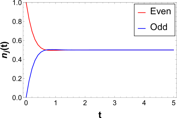
Figure 1: Relaxation of $n_{j}(t)$ for odd/even sites towards the steady state value from an initial Néel state. Calculated for $J_{+}=1.0,J_{-}=0.9$.

5 Two defect sector

We now turn to the defect sector problem. The Lindbladian in the sector with $q$ defects can be written as a sum over quadratic open chain Lindbladians of the form

$${\cal L}_{M}=-J_{+}(M+1)+\sum_{j=1}^{M-1}\Big{\{}J_{2}c^{\dagger}_{j}c_{j+1}+J_{1}c^{\dagger}_{j+1}c_{j}-J_{+}\left(c^{\dagger}_{j+1}c^{\dagger}_{j}+c_{j}c_{j+1}\right)\Big{\}}.$$ (79)

As these are not Hermitian the standard analysis of Lieb, Schultz and Mattis [86] for diagonalizing Hamiltonians quadratic in fermionic creation/annihilation operators does not apply. We therefore proceed as in Section 4.1, but find it advantageous to switch to Majorana fermions [15]

$$a_{2j-1}=c_{j}+c_{j}^{\dagger}\ ,\quad a_{2j}=i(c_{j}-c_{j}^{\dagger}).$$ (80)

In terms of the Majorana operators ${\cal L}_{M}$ is expressed as

$${\cal L}_{M}=-(M+1)J_{+}+\frac{1}{4}a\cdot A\cdot a,$$ (81)

where here and elsewhere $(\cdot)$ represents the dot product with no complex conjugation- that is, $a\cdot A\cdot a=\sum_{ij}a_{i}A_{ij}a_{j}$. $A$ is a $2M\times 2M$ anti-symmetric, block tridiagonal matrix equal to $A=K\otimes C-K^{T}\otimes C^{T}$ where $K_{jk}=\delta_{j,k-1}$ and $C$ is given by

$$C=\begin{pmatrix}J_{-}&-2iJ_{+}\cr 0&J_{-}\end{pmatrix}.$$ (82)

Assuming $A$ to be diagonalizable, anti-symmetry ensures its eigenvalues come in pairs $\pm\beta_{j}$ which we order as $\beta_{1},-\beta_{1}\dots$. We then normalize the eigenvectors according to

$$\vec{v}_{r}\cdot\vec{v}_{s}=(\sigma^{x}\otimes\mathbbm{1})_{rs}\ .$$ (83)

In fact, the complex eigenvalues also come in complex conjugate pairs. This can be seen by noting that one obtains $A^{*}$ from $A$ by conjugating $C$ by $\sigma^{z}$. In particular this means that if $A\vec{v}=\beta\vec{v}$ then also

$$A(\mathbbm{1}_{n}\otimes\sigma^{z})\vec{v}^{*}=\beta^{*}(\mathbbm{1}_{n}\otimes\sigma^{z})\vec{v}^{*}\ .$$ (84)

Finally we define new fermion operators by

$$b_{j}=\vec{v}_{2j-1}\cdot{\bf a}/\sqrt{2}\ ,\quad b^{\prime}_{j}=\vec{v}_{2j}\cdot{\bf a}/\sqrt{2}.$$ (85)

These fulfil simple anticommutation relations due to (83)

$$\{b_{j},b_{k}\}=0=\{b^{\prime}_{j},b^{\prime}_{k}\}\ ,\quad\{b_{j},b^{\prime}_{k}\}=\delta_{j,k}\ ,$$ (86)

and diagonalise the Lindbladian

$${\cal L}_{M}=-(M+1)J_{+}+\frac{1}{2}\sum_{k}\beta_{k}-\sum_{k}\beta_{k}b^{\prime}_{k}b_{k}.$$ (87)

For the matrix $A$ in our problem it is not a simple matter to find a closed form analytic expression for the spectrum, but we can gain insight into what the solutions look like by deforming our Lindbladian by adding a boundary term $J_{-}(n_{1}-n_{L})$. We stress that the resulting Lindbladian is unphysical. Then the matrix $A$ is modified to $A^{\prime}$

$$A^{\prime}=\begin{pmatrix}B&-C^{\rm T}&0&\dots&0\cr C&0&-C^{\rm T}&0&\vdots\cr 0&C&0&\ddots&0\cr\vdots&0&\ddots&0&-C^{\rm T}\cr 0&\dots&0&C&-B\end{pmatrix}\ ,\quad B=-iJ_{-}\begin{pmatrix}0&1\cr-1&0\end{pmatrix}.$$ (88)

It is now straightforward to obtain the eigenvectors of the matrix $A^{\prime}$. We make an ansatz $\vec{v}=(v_{1},v_{2},\dots)^{\rm T}$ where

$$v_{n}=z^{n}\begin{pmatrix}1\cr iz\end{pmatrix}+A_{z}(-1)^{n}z^{-n}\begin{pmatrix}1\cr-iz^{-1}\end{pmatrix}\ .$$ (89)

For this to be an eigenvector we require $A_{z}=z^{2}$ and $z$ to satisfy

$$0=(z^{2M}-(-1)^{M})(\Delta z^{2}-2z-\Delta).$$ (90)

The associated eigenvalues are then given by

$$\lambda_{z}=2J_{+}+J_{-}(z^{-1}-z).$$ (91)

This only gives rise to $M$ linearly independent eigenvectors, all with non-negative eigenvalues. We however get the full spectrum using this ansatz by reflecting in the imaginary axis. Thus in this case we find that the positive real part eigenvalues consist of $M-1$ values of $z$ that are roots of unity $z=e^{-ik}$ which recovers the periodic boundary condition result. There are also two eigenvalues that are exactly $0$ - for our actual boundary conditions these become two small real eigenvalues $\pm\lambda_{0}$ (they cannot be complex as the requirement that $\beta^{*}$ is an eigenvalue would then give four nearly zero eigenvalues which is too many). We plot the eigenvalues in the complex plane in Figure 2 for both $A$ and $A^{\prime}$ to highlight the impact of removing the boundary potential.

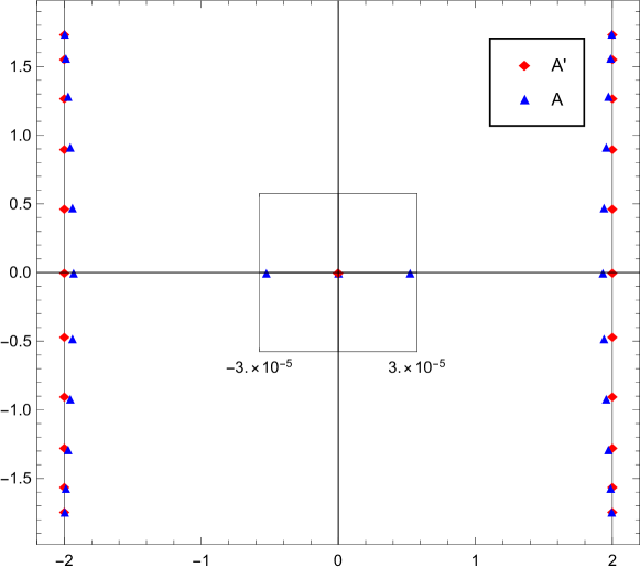
Figure 2: Eigenvalues of A’ (red diamonds), A (blue triangles) for $L=12,J_{+}=1.0,J_{-}=0.9$. Central inset is magnified such that both axes run from $\pm 3\times 10^{-5}$.

6 Transverse correlation function

We now turn to observables that involve defects. We focus on the particular example of an initial product state with ferromagnetic order along some direction in spin space

$$|\psi(0)\rangle=\left(1+|\alpha|^{2}\right)^{-L/2}\bigotimes_{m=1}^{L}\big{[}|\uparrow\rangle+\alpha|\downarrow\rangle\big{]}_{m}.$$ (92)

Our aim is to determine

$$S_{0,\ell+1}^{+-}=\Tr\left[\rho(t)\sigma^{+}_{L}\sigma^{-}_{\ell+1}\right].$$ (93)

As we showed above in (17) this involves only the projection of $|\rho(t)\rangle$ onto the subspace with two defects

$$S_{0,\ell+1}^{+-}=\langle\!\langle\mathbbm{1}_{\rm cl}|\sigma^{+}_{0}\sigma^{-}_{\ell+1}\Pi_{0,\ell+1}|\rho(t)\rangle\!\rangle=\langle\!\langle\mathbbm{1}_{\rm cl}|\sigma^{+}_{0}\sigma^{-}_{\ell+1}e^{{\cal L}t}\Pi_{0,\ell+1}|\rho(0)\rangle\!\rangle,$$ (94)

where

$$\Pi_{0,\ell+1}=E_{0}^{33}\otimes_{j=1}^{\ell}P_{j}E_{\ell+1}^{22}\otimes_{k=\ell+2}^{L-1}P_{k}\ .$$ (95)

Applying $\Pi_{0,\ell+1}$ to the initial density matrix $|\rho(0)\rangle\!\rangle=|\psi(0)\rangle\langle\psi(0)|$ gives

$$\Pi_{0,\ell+1}|\rho(0)\rangle\!\rangle=(1+|\alpha|^{2})^{-L}|\alpha|^{2}|3\rangle\!\rangle_{L}\otimes|\rho_{[1,\ell]}\rangle\!\rangle\otimes|2\rangle\!\rangle_{\ell+1}\otimes|\rho_{[\ell+2,L-1]}\rangle\!\rangle,$$ (96)

where

$$|\rho_{[a,b]}\rangle\!\rangle\equiv\otimes_{m=a}^{m=b}\left[|1\rangle\!\rangle+|\alpha|^{2}|4\rangle\!\rangle\right]_{m}.$$ (97)

We now see that the transverse spin-spin correlation function reduces in this initial state to

$$\Tr\left[\rho(t)\sigma^{+}_{1}\sigma^{-}_{\ell}\right] =\gamma(1+\gamma)^{-L}\tilde{G}_{\ell}(t)\tilde{G}_{L-\ell-2}(t)$$

$$\tilde{G}_{N}(t) =\langle\!\langle\mathbbm{1}_{[1,N]}|e^{{\cal L}_{N}t}|\rho_{[1,N]}\rangle\!\rangle.$$ (98)

Here we have defined $\gamma=|\alpha|^{2}$ since all quantities depend only on $\gamma$ and have separated out an overall factor $\gamma(1+\gamma)^{N}$ for convenience.

The propagators $\tilde{G}$ are defined on the finite chains discussed in Section 5 and can be expressed in terms of fermions as

$$\tilde{G}_{N}(t)={\phantom{\Big{\rangle}\!\Big{\rangle}}}_{0}\Big{\langle}\!\Big{\langle}0\Big{|}\prod_{j=0}^{N-1}\big{(}1+c_{N-j}\big{)}e^{{\cal L}_{N}t}\prod_{k=1}^{N}\big{(}1+\gamma c^{\dagger}_{k}\big{)}\Big{|}0\Big{\rangle}\!\Big{\rangle}_{0}\ .$$ (99)

As shown in A we can rewrite this as

$$\tilde{G}_{N}(t)={}_{0}\langle\!\langle 0|(1+X)e^{Y}e^{{\cal L}_{N}t}e^{\gamma^{2}Y^{\dagger}}(1+\gamma X^{\dagger})|0\rangle\!\rangle_{0}\ ,$$ (100)

where

$$X=\sum_{j=1}^{N}c_{j}\ ,\quad Y=\sum_{n<m}c_{m}c_{n}\ .$$ (101)

Using fermion parity conservation this simplifies to

$$\tilde{G}_{N}(t)={}_{0}\langle\!\langle 0|e^{Y}e^{{\cal L}_{N}t}e^{\gamma^{2}Y^{\dagger}}|0\rangle\!\rangle_{0}+\gamma\ {}_{0}\langle\!\langle 0|Xe^{Y}e^{{\cal L}_{N}t}e^{\gamma^{2}Y^{\dagger}}X^{\dagger}|0\rangle\!\rangle_{0}\ .$$ (102)

The two terms above can be written in the form

$$\tilde{G}^{(\alpha)}_{N}=\Tr\left[\tilde{\rho}^{(\alpha)}e^{Y}e^{{\cal L}_{N}t}e^{\gamma^{2}Y^{\dagger}}\right],\quad\alpha=1,2\ ,$$ (103)

where $e^{Y}$,$e^{{\cal L}_{N}t}$, $e^{\gamma^{2}Y^{\dagger}}$ are all manifestly Gaussian as are the $\tilde{\rho}^{(\alpha)}$ since they are the ground states of the quadratic Hamiltonians

$$H_{1}=\sum_{j=1}^{N}n_{j}\ ,\quad H_{2}=-n(p=0)+\sum_{p\neq 0}n(p)\ .$$ (104)

Thus (103) is now in the form of the trace of a product of Gaussian operators and can be evaluated. The procedure for this is given in detail in A. Here we outline the two key steps to the evaluation. The first step is to realise that since a product of Gaussian operators is Gaussian, we have

$$\rho^{(\alpha)}=\frac{e^{\gamma^{2}Y^{\dagger}}\tilde{\rho}^{(\alpha)}e^{Y}}{Z^{(\alpha)}}=\frac{1}{\mathcal{Z}(W^{(\alpha)})}e^{a\cdot W^{(\alpha)}\cdot a/4}.$$ (105)

Here, $Z^{(\alpha)}$ and ${\cal Z}(W^{(\alpha)})$ are two different normalisation factors defined each defined such that $\Tr\rho^{(a)}=1$. The $Z^{(a)}$ are calculated in B and given by 134. Writing the time evolution operator in the form

$$e^{{\cal L}_{N}t}=e^{\frac{1}{4}a\cdot A_{N}\cdot a}\ ,$$ (106)

we then obtain the following expression for the propagators (cf. A )

$$\Tr\left[\rho^{(\alpha)}e^{\frac{1}{4}a\cdot A_{N}\cdot a}\right]=Z^{(\alpha)}\left(\frac{{\rm det}(e^{W^{(\alpha)}}e^{A_{N}}+e^{-A_{N}}e^{-W^{(\alpha)}}+2)}{{\rm det}(e^{W^{(\alpha)}}+e^{-W^{(\alpha)}}+2)}\right)^{1/4}\ .$$ (107)

The second step is to use the fact that a Gaussian is determined by its second moments to change from working with the density matrix $e^{a\cdot W\cdot a/4}$ itself to instead working with its correlation matrix $\Gamma_{mn}=\Tr[\rho a_{n}a_{m}]-\delta_{mn}$. We calculate the latter in B by rewriting the trace as an inner product which can be evaluated in terms of Jordan-Wigner spins. Once $\Gamma$ is found $W$ is obtained through $\Gamma=\tanh\frac{W}{2}$, or equivalently

$$e^{W}=(1-\Gamma)^{-1}(1+\Gamma).$$ (108)

This then leads to an apparent difficulty since the correlation matrices corresponding to $\rho^{(\alpha)}$ (which are fixed through our choice of initial condition) satisfy $(\Gamma^{(\alpha)})^{2}=1$, implying that they have only eigenvalues equal to $\pm 1$ and the method set out above appears to break down. This issue can be dealt with by noting that

$$\Gamma^{(\alpha)}=\Pi^{(\alpha)}_{+}-\Pi^{(\alpha)}_{-}\ ,$$ (109)

where $\Pi^{(\alpha)}_{\pm}$ are projectors onto the two $N$ dimensional subspaces corresponding to eigenvalues $1$ and $-1$ of $\Gamma^{(\alpha)}$ respectively. These would correspond to eigenvalues $\pm\infty$ in $W$, which we regulate by setting them equal to $\pm\Lambda$ and taking the limit $\Lambda\to\infty$ in the end of the calculation. That is, we put:

$$e^{W^{(\alpha)}/2}=e^{\Lambda/2}\Pi^{(\alpha)}_{+}+e^{-\Lambda/2}\Pi^{(\alpha)}_{-}\ ,$$ (110)

which simplifies (107) to read

$$\Tr\left[\rho^{(\alpha)}e^{\frac{1}{4}a\cdot A_{N}t\cdot a}\right] =\left({\rm det}(\Pi^{(\alpha)}_{+}e^{A_{N}t}+\Pi^{(\alpha)}_{-}e^{-A_{N}t})\right)^{1/4}\equiv d^{(\alpha)}_{N}\ .$$ (111)

This yields a simple expression for the propagator

$$\tilde{G}_{N}(t)= e^{-J_{+}(N+1)t}\Big{[}Z^{(1)}d^{(1)}_{N}+\gamma Z^{(2)}d^{(2)}_{N}\Big{]}.$$ (112)

Substituting this into (98) then gives the transverse correlation function

$$S^{+-}_{0,\ell+1}(t)=\frac{\gamma}{(1+\gamma)^{L}} e^{-J_{+}Lt}\left(Z^{(1)}d_{\ell}^{(1)}+\gamma Z^{(2)}d_{\ell}^{(2)}\right)$$ (113)

$$\times\left(Z^{(1)}d_{L-\ell-2}^{(1)}+\gamma Z^{(2)}d_{L-\ell-2}^{(2)}\right).$$

The determinants $d^{(\alpha)}_{N}$ can now be straightforwardly computed numerically. In Fig. 3 we plot the transverse correlator at separation $2$, $S^{+-}_{0,2}(t)$, as a function of time.

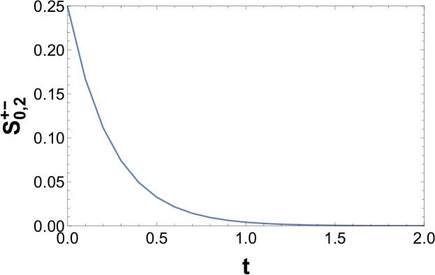
Figure 3: Full correlation function $S^{+-}_{0,2}(t)$ for $L=30$ sites, $J_{-}=0.9,J_{+}=1.0$ and $\gamma=0.9$.

We observe that the correlator decays quite quickly, and monotonically, from its initial value. We note however that this is the full correlation function and that more physically interesting is the connected correlator

$$S^{+-}_{\ell+1,C}=\Tr[S^{+}_{0}S^{-}_{\ell+1}\rho(t)]-\Tr[S^{+}_{0}\rho(t)]\Tr[S^{-}_{\ell+1}\rho(t)].$$ (114)

Here we have use the translation invariance of our initial condition to express the correlation function in terms of only the distance between the defects (note that this is $\ell+1$ and not $\ell$). The one point functions depend on the same propagators as the 2-point functions since

$${\rm Tr}[S^{+}_{0}\rho(t)]=\langle\!\langle\mathbbm{1}_{\rm cl}|E^{13}_{0}E^{24}_{0}|\rho(t)\rangle\!\rangle=\frac{\alpha}{1+\gamma}G_{L-1},$$ (115)

which gives

$$S^{+-}_{\ell+1,C}=\frac{\gamma}{(1+\gamma)^{2}}\left[G_{\ell}G_{L-\ell-2}-G_{L-1}^{2}\right].$$ (116)

Where we have expressed this in terms of $G_{N}=(1+\gamma)^{-N}\tilde{G}_{N}$ as this is more natural. In particular, since our initial state was a product state we have $G_{N}(0)=1$ for all $N$ and so the connected correlation function is initially $0$, indicating no correlations. We then expect that the Lindblad evolution will correlate neighbouring sites. This is countered by the fact that the steady state values of observables are all governed by the diagonal subspace values and so the connected correlations must go to zero at long times. In Figure 4(a) we plot the connected correlation between sites $1$ and $3$. We are able to observe that the dissipative dynamics does produce some correlations although they are small. Given that they also exponentially decay, the correlation generation would most likely not be visible had we started in an initially correlated state. In Figure 4(b) we plot the corresponding values for varying site separations and note an approximately exponential decrease with distance. We perform these calculations for total chain lengths of $L=30$, one might wonder if this is large enough to be essentially in the thermodynamic limit (in the sense that finite size effects are small enough to neglect). In fact, we find that the numerical values of the connected correlator vary very little as we increase $L$ so long as it is larger than twice the separation $\ell+1$. To show this we plot the connected correlator for $\ell=3$ for $L=8,9,10$ in Figure 5(a). Since the difference between the result for $9,10$ is too small to be visible, we plot the residual (along with the corresponding residual for $L=10,11$) in Figure 5(b).

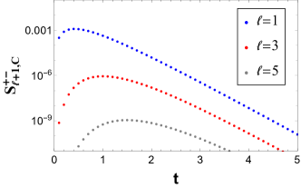
(a)  (b)

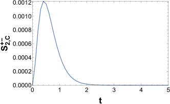
Figure 4: Connected correlation function for chain length $L=30$ and $J_{-}=0.9,J_{+}-1.0,\gamma=0.9$. (a) Connected correlations decay exponentially with separation $d=\ell+1$. (b) Connected correlation function for $\ell=1$, showing correlation generation.

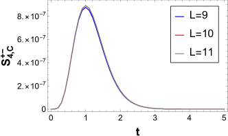
(a)  (b)

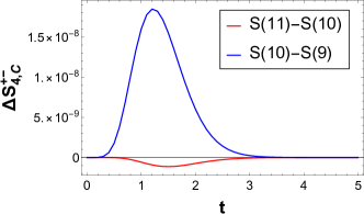
Figure 5: Finite size effects for $\ell=3$. $J_{-}=0.9,J_{+}-1.0,\gamma=0.9$: (a) Correlation function for three different chain lengths $L=8,9,10$. (b) Residuals between correlation function at $L=9,10$ and $L=10,11$.

7 Conclusions

We have considered a dissipative many-particle quantum system described by a Lindblad equation that for particular initial conditions reduces to an asymmetric simple exclusion process with additional pair creation and annihilation terms. The Lindbladian exhibits operator-space fragmentation and for particular pair creation/annihilation rates the model can be mapped to free fermions. The model thus extends the class of solvable Lindblad systems and in particular provides a concrete example of a setting where operator-space fragmentation can be used to compute correlation functions exactly. We have restricted attention to initial product states in order to make calculations simpler as well as to allow us to see the generation of correlations through dissipation in our model. Even though the initial states we have considered here are quite simple the analysis is not straightforward. It would be interesting to attempt to generalize our analysis to the case of entangled initial states. It would also be interesting to study the time evolution of entanglement measures such as entanglement negativity within this model.

Appendix A Fermion identities

A.1 Mixed parity fermion products

To arrive at Eq (100) the key identity is that for any collection of mutually anti-commuting variables $\{\zeta_{i}\}_{i=1}^{N}$ the following holds

$$\prod_{i=1}^{N}(1+\zeta_{i})=\left(1+\sum_{i=1}^{N}\zeta_{i}\right)\prod_{1\leq j<k\leq N}(1+\zeta_{j}\zeta_{k}).$$ (117)

This identity immediately provides a convenient decomposition into even and odd fermion parity parts. It can be proven by focussing on the odd and even components and using induction. To do so note that the even terms have the form

$$\mathbf{E}\left[\prod_{i=1}^{N}(1+\zeta_{i})\right]=\sum_{\genfrac{}{}{0.0pt}{}{k\text{ even}}{k\leq N}}\left(\sum_{1\leq i_{1}<\dots<i_{k}\leq N}\zeta_{i_{1}}\dots\zeta_{i_{k}}\right).$$ (118)

The counterpart for the odd terms is completely analogous. When multiplying this by $\sum_{j=1}^{N}\zeta_{j}$ the result will be a sum of $(N-k)\binom{N}{k}$ non-zero terms, each of which contain $k+1$ distinct $\zeta$’s. Moreover, in each term $k$ of the $\zeta$’s will be in ascending order by construction, with the final one appearing in each possible position. Thus $k/2$ pairs will cancel and the remaining $\frac{(N-k)}{k+1}\binom{N}{k}=(N-k-1)\binom{N}{k+1}$ terms are precisely those in the corresponding expansion of the odd part. We thus need only prove by induction the statement about the even terms

$$\sum_{k=2m}\left(\sum_{1\leq i_{1}<\dots<i_{k}\leq N}\zeta_{i_{1}}\dots\zeta_{i_{k}}\right)=\prod_{1\leq j<k\leq N}(1+\zeta_{j}\zeta_{k})\ .$$ (119)

To this end we assume the induction hypothesis up to $N-1$ and notice that for $N$ sites we can rewrite the product of quadratic terms as

$$\prod_{i<j}^{N-1}(1+\zeta_{i}\zeta_{j})\prod_{\omega=1}^{N-1}(1+\zeta_{\omega}\zeta_{N})=\prod_{i<j}^{N-1}(1+\zeta_{i}\zeta_{j})(1+\sum_{\omega=1}^{N-1}\zeta_{\omega}\zeta_{N}).$$ (120)

We then use the induction hypothesis on the first factor on the right hand side. When multiplied by the second factor two things can happen: (i) it gets multiplied by 1, thus generating all possible even terms not including $\zeta_{N}$, (ii) it gets multiplied by $(\sum_{\omega=1}^{N-1}\zeta_{\omega})\zeta_{N}$. For the latter note that multiplying by $\sum\zeta_{\omega}$ generates all possible odd expressions without $\zeta_{N}$ and multiplying by $\zeta_{N}$ at the end then gives the desired result. Along with the observation that the base case of $N=0$ is trivial this completes the proof of (117).

In the context of Eq (100) we set $\zeta_{i}=\gamma c_{i}^{\dagger}$ so that we have

$$\prod_{k=1}^{N}(1+\gamma c_{k}^{\dagger})=\prod_{1\leq m<n\leq N}(1+\gamma^{2}c_{m}^{\dagger}c_{n}^{\dagger})(1+\gamma\sum_{k=1}^{N}c_{k}^{\dagger})\ .$$ (121)

This is the desired simplification upon defining $X,Y$ in the main text and applying the standard result that $e^{Y^{\dagger}}=\prod_{m<n}(1+c^{\dagger}_{m}c^{\dagger}_{n})$ where $Y^{\dagger}=\sum_{m<n}c_{m}^{\dagger}c_{n}^{\dagger}$.

A.2 Trace of Gaussian operators

The main result required in the derivation of (107) is the identity [87]

$$\Tr[e^{a\cdot W\cdot a/4}]=\sqrt{{\rm det}(e^{W/2}+e^{-W/2})}.$$ (122)

Here $a_{j}$ are Majorana fermions and $W$ an antisymmetric matrix. We note that (122) is easy to establish if $W$ is diagonalizable. In that case its eigenvalues come in pairs $\pm\beta_{k}$ and the left hand side becomes

$$\Tr[e^{\sum_{k}\beta_{k}(\frac{1}{2}-n_{k})}]=\prod_{\text{Re}\beta_{k}>0}\left[e^{\beta_{k}/2}+e^{-\beta_{k}/2}\right].$$ (123)

Because $W$ is anti-symmetric, its eigenvalues come in $\pm$ pairs and so the determinant contains exactly two copies of each factor on the right hand side of (123). This then establishes (122). If $W$ is not diagonalizable then we define

$$f[W]=\Tr[e^{a\cdot W\cdot a/4}]-\sqrt{\det(e^{W/2}+e^{-W/2})}.$$ (124)

Since $f[W]=0$ for all diagonalisable matrices (which is a dense subset of all matrices) and $f$ is a continuous function, we have $f=0$ identically.

We also make heavy use of a result following from the Baker-Campbell-Hausdorff formula, namely that for Majorana fermions $a_{j}$ normalised such that $\{a_{i},a_{j}\}=2\delta_{ij}$

$$e^{\frac{1}{4}a\cdot W_{1}\cdot a}e^{\frac{1}{4}a\cdot W_{2}\cdot a}=e^{\frac{1}{4}a\cdot W_{3}\cdot a}\ ,$$ (125)

where $e^{W_{3}}=e^{W_{1}}e^{W_{2}}$. Along with (122) this allows us to write

$$\Tr[e^{\frac{1}{4}a\cdot W_{1}\cdot a}e^{\frac{1}{4}a\cdot W_{2}\cdot a}] =\sqrt{{\rm det}(e^{W_{3}/2}+e^{-W_{3}/2})}$$ (126)

$$=\big{[}{\rm det}(e^{W_{3}}+e^{-W_{3}}+2)\big{]}^{1/4}\ .$$

Appendix B Correlation matrices

The two correlation matrices we need are given by the inner products

$$\Gamma^{(1)}_{mn}+\delta_{mn} =\frac{\langle\!\langle 0|e^{Y}a_{n}a_{m}e^{\gamma^{2}Y^{\dagger}}|0\rangle\!\rangle}{\langle\!\langle 0|e^{Y}e^{\gamma^{2}Y^{\dagger}}|0\rangle\!\rangle}\ ,$$ (127)

$$\Gamma^{(2)}_{mn}+\delta_{mn} =\frac{\langle\!\langle 0|Xe^{Y}a_{n}a_{m}e^{\gamma^{2}Y^{\dagger}}X^{\dagger}|0\rangle\!\rangle}{\langle\!\langle 0|Xe^{Y}e^{\gamma^{2}Y^{\dagger}}X^{\dagger}|0\rangle\!\rangle}.$$ (128)

The denominators are equal to the normalization factors $Z^{(1)},Z^{(2)}$ that appear in the final result (113). Both numerators and denominators can be found by making use of (117) in the form

$$\prod_{j=1}^{N}\left(1+\gamma c_{k}^{\dagger}\right)+\prod_{j=1}^{N}\left(1-\gamma c_{k}^{\dagger}\right)= 2e^{\gamma^{2}Y^{\dagger}}\ ,$$ (129)

$$\prod_{j=1}^{N}\left(1+\gamma c_{k}^{\dagger}\right)-\prod_{j=1}^{N}\left(1-\gamma c_{k}^{\dagger}\right)= 2\gamma Xe^{\gamma^{2}Y^{\dagger}}\ .$$ (130)

Using (130) we can express the correlation matrices as

$$\Gamma^{(1)}_{mn}+\delta_{mn} =\frac{g^{++}_{mn}+g^{+-}_{mn}}{Z^{++}+Z^{+-}}\ ,\quad\Gamma^{(2)}_{mn}+\delta_{mn}=\frac{g^{++}_{mn}-g^{+-}_{mn}}{Z^{++}-Z^{+-}}\ ,$$ (131)

where we have defined

$$g^{\sigma\sigma^{\prime}}_{mn}= \langle\!\langle 0|\prod_{j=0}^{N-1}(1+\sigma c_{N-j})a_{n}a_{m}\prod_{k=1}^{N}(1+\sigma^{\prime}\gamma c_{k}^{\dagger})|0\rangle\!\rangle\ ,$$ (132)

$$Z^{\sigma\sigma^{\prime}}= \langle\!\langle 0|\prod_{j=0}^{N-1}(1+\sigma c_{N-j})\prod_{k=1}^{N}(1+\sigma^{\prime}\gamma c_{k}^{\dagger})|0\rangle\!\rangle\ .$$ (133)

A simple calculation then gives that $g_{mn}^{++}=g_{mn}^{--}$ and $g_{mn}^{+-}=g_{mn}^{-+}$ and likewise for $Z^{\sigma\sigma^{\prime}}$. Explicit expressions for $g_{mn}^{\sigma\sigma^{\prime}}$ and $Z^{\sigma\sigma^{\prime}}$ are readily obtained by reverting to their respective representations in terms of spins (i.e. undoing the Jordan-Wigner transformation). We find

$$Z^{(1)}=\frac{1}{2}\left[(1+\gamma)^{N}+(1-\gamma)^{N}\right]\ ,$$

$$Z^{(2)}=\frac{1}{2}\left[(1+\gamma)^{N}-(1-\gamma)^{N}\right],$$ (134)

and $\Gamma^{(\alpha)}$ are anti-symmetric $2N\times 2N$ block matrices of the form

$$\Gamma^{(\alpha)}=\frac{1}{x^{N}-(-1)^{\alpha}y^{N}}\begin{pmatrix}\Gamma_{0}^{(\alpha)}&-(\Gamma^{(\alpha)}_{1})^{\rm T}&\dots&-(\Gamma^{(\alpha)}_{N-1})^{\rm T}\cr\Gamma_{1}^{(\alpha)}&\Gamma_{0}^{(\alpha)}&\dots&\vdots\cr\vdots&\dots&\dots&\vdots\cr\Gamma_{N-1}^{(\alpha)}&\dots&\dots&\Gamma_{0}^{(\alpha)}\end{pmatrix}\ ,\quad\alpha=1,2.$$ (135)

The $2\times 2$ blocks are given by

$$\Gamma^{(\alpha)}_{0} =\begin{pmatrix}0&i(f_{N-1}\pm f_{1})\cr-i(f_{N-1}-(-1)^{\alpha}f_{1})&0\end{pmatrix}\ ,$$

$$\Gamma^{(\alpha)}_{a} =\begin{pmatrix}f_{N-a}-(-1)^{\alpha}f_{a}&-i(f_{a-1}-(-1)^{\alpha}f_{N-a+1})\cr-i(f_{a+1}-(-1)^{\alpha}f_{N-a-1})&-(f_{N-a}-(-1)^{\alpha}f_{a})\end{pmatrix}\ ,$$ (136)

where we have defined

$$x=1+\gamma\ ,\quad y=1-\gamma\ ,\quad f_{a}=x^{a}y^{N-a}\ .$$ (137)

One can verify that $(\Gamma^{(\alpha)})^{2}=\mathbbm{1}$. Since $\Gamma^{(\alpha)}$ is anti-symmetric it therefore has equal numbers of eigenvalues $\pm 1$, which we used in the main text. The eigenvectors depend on $x,y$ and we find these numerically to determine the correct projectors to use.

References

- [1] V. Gorini, A. Kossakowski, and E. C. G. Sudarshan, Completely positive dynamical semigroups of N-level systems J. Math. Phys. 17 no. 5, (1976) 821–825.
- [2] G. Lindblad, On the generators of quantum dynamical semigroups Comm. Math. Phys. 48 no. 2, (1976) 119–130.
- [3] H.-P. Breuer and F. Petruccione, The theory of open quantum systems. Oxford University Press on Demand, 2002.
- [4] A. C. Li, F. Petruccione, and J. Koch, Perturbative approach to Markovian open quantum systems Sci. Rep. 4 (2014) 4887.
- [5] L. M. Sieberer, M. Buchhold, and S. Diehl, Keldysh field theory for driven open quantum systems Rep. Prog. Phys. 79 no. 9, (2016) 096001.
- [6] A. J. Daley, Quantum trajectories and open many-body quantum systems Adv. Phys. 63 no. 2, (2014) 77–149.
- [7] L. Bonnes and A. M. Läuchli, Superoperators vs. trajectories for matrix product state simulations of open quantum system: a case study arXiv:1411.4831.
- [8] J. Cui, J. I. Cirac, and M. C. Bañuls, Variational Matrix Product Operators for the Steady State of Dissipative Quantum Systems Phys. Rev. Lett. 114 (Jun, 2015) 220601.
- [9] A. H. Werner, D. Jaschke, P. Silvi, M. Kliesch, T. Calarco, J. Eisert, and S. Montangero, Positive Tensor Network Approach for Simulating Open Quantum Many-Body Systems Phys. Rev. Lett. 116 (Jun, 2016) 237201.
- [10] H. Weimer, A. Kshetrimayum, and R. Orús, Simulation methods for open quantum many-body systems Rev. Mod. Phys. 93 (Mar, 2021) 015008.
- [11] P. Calabrese, F. H. Essler, and G. Mussardo, Introduction to ‘quantum integrability in out of equilibrium systems’ J. Stat. Mech. 2016 no. 6, (2016) 064001.
- [12] F. H. L. Essler and M. Fagotti, Quench dynamics and relaxation in isolated integrable quantum spin chains J. Stat. Mech. 2016 no. 6, (2016) 064002.
- [13] P. Calabrese and J. Cardy, Quantum quenches in 1+ 1 dimensional conformal field theories J. Stat. Mech. 2016 no. 6, (2016) 064003.
- [14] V. Alba, B. Bertini, M. Fagotti, L. Piroli, and P. Ruggiero, Generalized-hydrodynamic approach to inhomogeneous quenches: correlations, entanglement and quantum effects arXiv:2104.00656.
- [15] T. Prosen, Third quantization: a general method to solve master equations for quadratic open Fermi systems New J. Phys. 10 no. 4, (2008) 043026.
- [16] J. Eisert and T. Prosen, Noise-driven quantum criticality arXiv:1012.5013 (2010) .
- [17] T. Prosen, Spectral theorem for the Lindblad equation for quadratic open fermionic systems J. Stat. Mech. 2010 no. 07, (2010) P07020.
- [18] S. Clark, J. Prior, M. Hartmann, D. Jaksch, and M. B. Plenio, Exact matrix product solutions in the Heisenberg picture of an open quantum spin chain New J. Phys. 12 no. 2, (2010) 025005.
- [19] B. Horstmann, J. I. Cirac, and G. Giedke, Noise-driven dynamics and phase transitions in fermionic systems Phys. Rev. A 87 (Jan, 2013) 012108.
- [20] M. Keck, S. Montangero, G. E. Santoro, R. Fazio, and D. Rossini, Dissipation in adiabatic quantum computers: lessons from an exactly solvable model New J. Phys. 19 no. 11, (2017) 113029.
- [21] E. Vernier, Mixing times and cutoffs in open quadratic fermionic systems SciPost Phys. 9 (2020) 49.
- [22] S. Maity, S. Bandyopadhyay, S. Bhattacharjee, and A. Dutta, Growth of mutual information in a quenched one-dimensional open quantum many-body system Phys. Rev. B 101 (May, 2020) 180301.
- [23] V. Alba and F. Carollo, Spreading of correlations in Markovian open quantum systems Phys. Rev. B 103 (Jan, 2021) L020302.
- [24] V. Eisler, Crossover between ballistic and diffusive transport: the quantum exclusion process J. Stat. Mech. 2011 no. 06, (2011) P06007.
- [25] B. Žunkovič, Closed hierarchy of correlations in Markovian open quantum systems New J. Phys. 16 no. 1, (2014) 013042.
- [26] S. Caspar, F. Hebenstreit, D. Mesterhazy, and U.-J. Wiese, Dissipative Bose–Einstein condensation in contact with a thermal reservoir New J. Phys. 18 no. 7, (2016) 073015.
- [27] S. Caspar, F. Hebenstreit, D. Mesterházy, and U.-J. Wiese, Dynamics of dissipative Bose-Einstein condensation Phys. Rev. A 93 (Feb, 2016) 021602.
- [28] D. Mesterházy and F. Hebenstreit, Solvable Markovian dynamics of lattice quantum spin models Phys. Rev. A 96 (Jul, 2017) 010104.
- [29] M. Foss-Feig, J. T. Young, V. V. Albert, A. V. Gorshkov, and M. F. Maghrebi, Solvable Family of Driven-Dissipative Many-Body Systems Phys. Rev. Lett. 119 (Nov, 2017) 190402.
- [30] I. Klich, Closed hierarchies and non-equilibrium steady states of driven systems Ann. Phys. 404 (2019) 66–80.
- [31] J. M. Torres, Closed-form solution of Lindblad master equations without gain Phys. Rev. A 89 (May, 2014) 052133.
- [32] M. Nakagawa, N. Kawakami, and M. Ueda, Exact Liouvillian Spectrum of a One-Dimensional Dissipative Hubbard Model Phys. Rev. Lett. 126 (Mar, 2021) 110404.
- [33] B. Buca, C. Booker, M. Medenjak, and D. Jaksch, Dissipative bethe ansatz: Exact solutions of quantum many-body dynamics under loss arXiv:2004.05955.
- [34] M. V. Medvedyeva, F. H. L. Essler, and T. Prosen, Exact Bethe Ansatz Spectrum of a Tight-Binding Chain with Dephasing Noise Phys. Rev. Lett. 117 (Sep, 2016) 137202.
- [35] D. A. Rowlands and A. Lamacraft, Noisy coupled qubits: Operator spreading and the Fredrickson-Andersen model Phys. Rev. B 98 (Nov, 2018) 195125.
- [36] N. Shibata and H. Katsura, Dissipative quantum Ising chain as a non-Hermitian Ashkin-Teller model Phys. Rev. B 99 (Jun, 2019) 224432.
- [37] N. Shibata and H. Katsura, Dissipative spin chain as a non-Hermitian Kitaev ladder Phys. Rev. B 99 (May, 2019) 174303.
- [38] A. A. Ziolkowska and F. H. L. Essler, Yang-Baxter integrable Lindblad equations SciPost Phys. 8 (2020) 044.
- [39] P. Ribeiro and T. Prosen, Integrable Quantum Dynamics of Open Collective Spin Models Phys. Rev. Lett. 122 (Jan, 2019) 010401.
- [40] S. Lerma-Hernández, A. Rubio-García, and J. Dukelsky, Trigonometric SU(N) Richardson–Gaudin models and dissipative multi-level atomic systems Journal of Physics A: Mathematical and Theoretical 53 no. 39, (Aug, 2020) 395302.
- [41] D. Yuan, H.-R. Wang, Z. Wang, and D.-L. Deng, Solving the Liouvillian Gap with Artificial Neural Networks Phys. Rev. Lett. 126 (Apr, 2021) 160401.
- [42] M. de Leeuw, C. Paletta, and B. Pozsgay, Constructing integrable Lindblad superoperators arXiv:2101.08279.
- [43] F. H. L. Essler and L. Piroli, Integrability of one-dimensional Lindbladians from operator-space fragmentation Phys. Rev. E 102 (Dec, 2020) 062210.
- [44] F. Spitzer, Interaction of Markov processes Adv. Math. 5 no. 2, (1970) 246 – 290.
- [45] T. M. Liggett, Interacting Particle Systems. Springer, New York, 1985.
- [46] B. Derrida, An exactly soluble non-equilibrium system: The asymmetric simple exclusion process Phys. Rep. 301 no. 1, (1998) 65 – 83.
- [47] G. M. Schütz, Exactly Solvable Models for Many-Body Systems Far From Equilibrium. in Phase Transitions and Critical Phenomena 19, pp. 1 - 251, C. Domb und J. Lebowitz (eds.) Academic Press, London, 2000.
- [48] T. Jin, A. Krajenbrink, and D. Bernard, From Stochastic Spin Chains to Quantum Kardar-Parisi-Zhang Dynamics Phys. Rev. Lett. 125 (Jul, 2020) 040603.
- [49] M. Bauer, D. Bernard, and T. Jin, Stochastic dissipative quantum spin chains (I) : Quantum fluctuating discrete hydrodynamics SciPost Phys. 3 (2017) 033.
- [50] M. Bauer, D. Bernard, and T. Jin, Equilibrium Fluctuations in Maximally Noisy Extended Quantum Systems SciPost Phys. 6 (2019) 45.
- [51] D. Bernard and T. Jin, Open Quantum Symmetric Simple Exclusion Process Phys. Rev. Lett. 123 (Aug, 2019) 080601.
- [52] D. Bernard and T. Jin, Solution to the Quantum Symmetric Simple Exclusion Process : the Continuous Case arXiv:2006.12222.
- [53] R. Frassek, C. Giardina, and J. Kurchan, Duality in quantum transport models arXiv:2008.03476.
- [54] L.-H. Gwa and H. Spohn, Six-vertex model, roughened surfaces, and an asymmetric spin Hamiltonian Phys. Rev. Lett. 68 (Feb, 1992) 725–728.
- [55] L.-H. Gwa and H. Spohn, Bethe solution for the dynamical-scaling exponent of the noisy Burgers equation Phys. Rev. A 46 (Jul, 1992) 844–854.
- [56] D. Kim, Bethe ansatz solution for crossover scaling functions of the asymmetric XXZ chain and the Kardar-Parisi-Zhang-type growth model Phys. Rev. E 52 (Oct, 1995) 3512–3524.
- [57] O. Golinelli and K. Mallick, Bethe ansatz calculation of the spectral gap of the asymmetric exclusion process J. Phys. A: Math. Gen. 37 no. 10, (2004) 3321.
- [58] J. de Gier and F. H. L. Essler, Bethe Ansatz Solution of the Asymmetric Exclusion Process with Open Boundaries Phys. Rev. Lett. 95 (Dec, 2005) 240601.
- [59] J. De Gier and F. H. L. Essler, Exact spectral gaps of the asymmetric exclusion process with open boundaries J. Stat. Mech. 2006 no. 12, (2006) P12011.
- [60] J. de Gier and F. H. L. Essler, Slowest relaxation mode of the partially asymmetric exclusion process with open boundaries J. Phys. A: Math. Theor. 41 no. 48, (2008) 485002.
- [61] K. Mallick, Some exact results for the exclusion process J. Stat. Mech. 2011 no. 01, (2011) P01024.
- [62] N. Crampé, E. Ragoucy, and D. Simon, Matrix coordinate Bethe ansatz: applications to XXZ and ASEP models J. Phys. A: Math. Theor. 44 no. 40, (2011) 405003.
- [63] J. E. Santos, G. M. Schütz, and R. B. Stinchcombe, Diffusion–annihilation dynamics in one spatial dimension J. Chem. Phys. no. 105, (1996) 2399.
- [64] P.-A. Bares and M. Mobilia, Solution of Classical Stochastic One-Dimensional Many-Body Systems Phys. Rev. Lett. 83 (Dec, 1999) 5214–5217.
- [65] M. Mobilia and P.-A. Bares, Exact solution of a class of one-dimensional nonequilibrium stochastic models Phys. Rev. E 63 (Apr, 2001) 056112.
- [66] N. Crampe, E. Ragoucy, V. Rittenberg, and M. Vanicat, Integrable dissipative exclusion process: Correlation functions and physical properties Phys. Rev. E 94 (Sep, 2016) 032102.
- [67] B. Derrida, M. R. Evans, and D. Mukamel, Exact diffusion constant for one-dimensional asymmetric exclusion models Journal of Physics A: Mathematical and General 26 no. 19, (Oct, 1993) 4911–4918.
- [68] L. Bertini, A. De Sole, D. Gabrielli, G. Jona-Lasinio, and C. Landim, Macroscopic Fluctuation Theory for Stationary Non-Equilibrium States J. Stat. Phys. 107 (2002) 635.
- [69] T. Bodineau and B. Derrida, Current Fluctuations in Nonequilibrium Diffusive Systems: An Additivity Principle Phys. Rev. Lett. 92 (May, 2004) 180601.
- [70] L. Bertini, A. De Sole, D. Gabrielli, G. Jona-Lasinio, and C. Landim, Current fluctuations in stochastic lattice gases Phys. Rev. Lett. 94 no. 3, (2005) 030601.
- [71] B. Derrida, Non-equilibrium steady states: fluctuations and large deviations of the density and of the current Journal of Statistical Mechanics: Theory and Experiment 2007 no. 07, (Jul, 2007) P07023–P07023.
- [72] J. de Gier and F. H. L. Essler, Large Deviation Function for the Current in the Open Asymmetric Simple Exclusion Process Phys. Rev. Lett. 107 (Jun, 2011) 010602.
- [73] A. Lazarescu and K. Mallick, An exact formula for the statistics of the current in the TASEP with open boundaries Journal of Physics A: Mathematical and Theoretical 44 no. 31, (Jul, 2011) 315001.
- [74] D. Bernard, F. H. L. Essler, L. Hruza, and M. Medenjak, Dynamics of Fluctuations in Quantum Simple Exclusion Processes arXiv:2107.02662.
- [75] V. Gritsev, E. Altman, E. Demler, and A. Polkovnikov, Full quantum distribution of contrast in interference experiments between interacting one-dimensional Bose liquids Nature Phys. 2 (2006) 705.
- [76] T. Kitagawa, A. Imambekov, J. Schmiedmayer, and E. Demler, The dynamics and prethermalization of one-dimensional quantum systems probed through the full distributions of quantum noise New Journal of Physics 13 no. 7, (Jul, 2011) 073018.
- [77] V. Eisler and Z. Rácz, Full Counting Statistics in a Propagating Quantum Front and Random Matrix Spectra Phys. Rev. Lett. 110 (Feb, 2013) 060602.
- [78] S. Groha, F. H. L. Essler, and P. Calabrese, Full counting statistics in the transverse field Ising chain SciPost Phys. 4 (2018) 43.
- [79] M. Collura, Relaxation of the order-parameter statistics in the Ising quantum chain SciPost Phys. 7 (2019) 72.
- [80] M. Collura and F. H. L. Essler, How order melts after quantum quenches Phys. Rev. B 101 (Jan, 2020) 041110.
- [81] R. Javier, V. Tortora, P. Calabrese, and M. Collura, Relaxation of the order-parameter statistics and dynamical confinement arXiv:2005.01679.
- [82] A. Ziolkowska and F. H. L. Essler, “Integrable generalizations of the quantum ASEP.” unpublished, 2020.
- [83] P. Sala, T. Rakovszky, R. Verresen, M. Knap, and F. Pollmann, Ergodicity Breaking Arising from Hilbert Space Fragmentation in Dipole-Conserving Hamiltonians Phys. Rev. X 10 (Feb, 2020) 011047.
- [84] V. Khemani, M. Hermele, and R. Nandkishore, Localization from Hilbert space shattering: From theory to physical realizations Phys. Rev. B 101 (May, 2020) 174204.
- [85] S. Moudgalya, A. Prem, R. Nandkishore, N. Regnault, and B. A. Bernevig, Thermalization and its absence within Krylov subspaces of a constrained Hamiltonian arXiv:1910.14048 [cond-mat.str-el].
- [86] E. Lieb, T. Schultz, and D. Mattis, Two soluble models of an antiferromagnetic chain Annals of Physics 16 no. 3, (1961) 407 – 466.
- [87] M. Fagotti and P. Calabrese, Entanglement entropy of two disjoint blocks in XY chains Journal of Statistical Mechanics: Theory and Experiment 2010 no. 04, (Apr, 2010) P04016.