Sparse Spiking Gradient Descent

Abstract

There is an increasing interest in emulating Spiking Neural Networks (SNNs) on neuromorphic computing devices due to their low energy consumption. Recent advances have allowed training SNNs to a point where they start to compete with traditional Artificial Neural Networks (ANNs) in terms of accuracy, while at the same time being energy efficient when run on neuromorphic hardware. However, the process of training SNNs is still based on dense tensor operations originally developed for ANNs which do not leverage the spatiotemporally sparse nature of SNNs. We present here the first sparse SNN backpropagation algorithm which achieves the same or better accuracy as current state of the art methods while being significantly faster and more memory efficient. We show the effectiveness of our method on real datasets of varying complexity (Fashion-MNIST, Neuromophic-MNIST and Spiking Heidelberg Digits) achieving a speedup in the backward pass of up to $150$x, and $85\%$ more memory efficient, without losing accuracy.

1 Introduction

In recent years, deep artificial neural networks (ANNs) have matched and occasionally surpassed human-level performance on increasingly difficult auditory and visual recognition problems [1, 2, 3], natural language processing tasks [4, 5] and games [6, 7, 8]. As these tasks become more challenging the neural networks required to solve them grow larger and consequently their power efficiency becomes more important [9, 10]. At the same time, the increasing interest in deploying these models into embedded applications calls for faster, more efficient and less memory intensive networks [11, 12].

The human brain manages to perform similar and even more complicated tasks while only consuming about 20W [13] which contrasts with the hundreds of watts required for running ANNs [9]. Unlike ANNs, biological neurons in the brain communicate through discrete events called spikes. A biological neuron integrates incoming spikes from other neurons in its membrane potential and after reaching a threshold emits a spike and resets its potential [14]. The spiking neuron, combined with the sparse connectivity of the brain, results in a highly spatio-temporally sparse activity [15] which is fundamental to achieve this level of energy efficiency.

Inspired by the extraordinary performance of the brain, neuromorphic computing aims to obtain the same level of energy efficiency preferably while maintaining an accuracy standard on par with ANNs by emulating spiking neural networks (SNNs) on specialised hardware [16, 17, 18, 19]. These efforts go in two directions: emulating the SNNs and training the SNNs. While there is a growing number of successful neuromorphic implementations for the former [20, 21, 22, 23, 24, 17, 25, 26], the latter has proven to be more challenging. Some neuromorphic chips implement local learning rules [26, 27, 28] and recent advances have achieved to approximate backpropagation on-chip [29]. However, a full end-to-end supervised learning via error backpropagation requires off-chip training [22, 23, 18]. This is usually achieved by simulating and training the entire SNN on a GPU and more recently, emulating the forward pass of the SNN on neuromorphic hardware and then performing the backward pass on a GPU [30, 31]. The great flexibility provided by GPUs allows the development of complex training pipelines without being constrained by neuromorphic hardware specifications. However, as GPUs do not leverage the event-driven nature of spiking computations this results in effective but slower and less energy efficient training. An alternative to directly training an SNN consists on training an ANN and converting it to an SNN. However, this approach has been recently shown to not be more energy efficient than using the original ANN in the first place [32].

Training SNNs has been a challenge itself even without considering a power budget due to the all-or-none nature of spikes which hinders traditional gradient descent methods [33, 34]. Since the functional form of a spike is a unit impulse, it has a zero derivative for all membrane potentials except at the threshold where it is infinity. Recently developed methods based on surrogate gradients have been shown to be capable of solving complex tasks to near state-of-the-art accuracies [35, 18, 36, 37, 38, 39, 31]. The problem of non-differentiability is solved by adopting a well-behaved surrogate gradient when backpropagating the error [33]. This method, while effective for training very accurate models, is still constrained to working on dense tensors, thus, not profiting from the sparse nature of spiking, and limits the training speed and power efficiency when training SNNs.

In this work we introduce a sparse backpropagation method for SNNs. Recent work on ANNs has shown that adaptive dropout [40] and adaptive sparsity [41] can be used to achieve state-of-the-art performance at a fraction of the computational cost [42, 43]. We show that by redefining the surrogate gradient functional form, a sparse learning rule for SNNs arises naturally as a three-factor Hebbian-like learning rule. We empirically show an improved backpropagation time up to $70$x faster than current implementations and up to $40\%$ more memory efficient in real datasets (Fashion-MNIST (F-MNIST) [44], Neuromorphic-MNIST (N-MNIST) [45] and Spiking Heidelberg Dataset (SHD) [46]) thus reducing the computational gap between the forward and backward passes. This improvement will not only impact training for neuromorphic computing applications but also for computational neuroscience research involving training on SNNs [39].

2 Sparse Spike Backpropagation

2.1 Forward Model

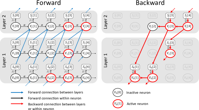
We begin by introducing the spiking networks we are going to work with (Figs. 1 and 2). For simplicity we have omitted the batch dimension in the derivations but it is later used on the complexity analysis and experiments. We have a total of $L$ fully connected spiking layers. Each layer $l$ consisting of $N^{(l)}$ spiking neurons which are fully connected to the next layer $l\!+\!1$ through synaptic weights $W^{(l)}\!\in\!\mathbb{R}^{N^{(l)}\times N^{(l\!+\!1)}}$. Each neuron has an internal state variable, the membrane potential, $V^{(l)}_{j}[t]\in\mathbb{R}$ that updates every discrete time step $t\in\{0,\ldots,T\!-\!1\}$ for some finite simulation time $T\!\in\!\mathbb{N}$. Neurons emit spikes according to a spiking function $f\colon\mathbb{R}\to\{0,1\}$ such that

$$S^{(l)}_{i}[t]\!=\!f(V^{(l)}_{i}[t])$$ (1)

Figure 1: Spiking Neural Network diagram highlighting the forward and backward passes

The membrane potential varies according to a simplified Leaky Integrate and Fire (LIF) neuron model in which input spikes are directly integrated into the membrane [14]. After a neuron spikes, its potential is reset to $V_{r}$. We will work with a discretised version of this model (see Appendix E for a continuous time version). The membrane potential of neuron $j$ in layer $l\!+\!1$ evolves according to the following difference equation

$$V^{(l\!+\!1)}_{j}[t\!+\!1]=\alpha(V^{(l+1)}_{j}[t]-V_{rest})+V_{rest}+\sum_{i}S^{(l)}_{i}[t]W^{(l)}_{ij}-(V_{th}-V_{r})S^{(l\!+\!1)}_{j}[t]$$ (2)

The first two terms account for the leaky part of the model where we define $\alpha=\exp(-\Delta t/\tau)$ with $\Delta t,\tau\in\mathbb{R}$ being the time resolution of the simulation and the membrane time constant of the neurons respectively. The second term deals with the integration of spikes. The last term models the resetting mechanism by subtracting the distance from the threshold to the reset potential. For simplicity and without loss of generality, we consider $V_{rest}\!=\!0,V_{th}\!=\!1,V_{r}\!=\!0$ and $V_{i}^{(l)}[0]\!=\!0\>\forall\>l,i$ from now on.

We can unroll (2) to obtain

$$V^{(l\!+\!1)}_{j}[t\!+\!1]=\underbrace{\sum_{i}\underbrace{{\color[rgb]{0,0.44,0.75}\sum_{k=0}^{t}\alpha^{t-k}S^{(l)}_{i}[k]}}_{\text{Input trace}}W^{(l)}_{ij}}_{\text{Weighted input}}-\underbrace{\sum_{k=0}^{t}\alpha^{t-k}S^{(l+1)}_{j}[k]}_{\text{Resetting term}}\vspace{-0.1cm}$$ (3)

Thus, a spiking neural network can be viewed as a special type of recurrent neural network where the activation function of each neuron is the spiking function $f(\cdot)$. The spiking function, is commonly defined as the unit step function centered at a particular threshold $V_{th}$

$$f(v)=\begin{cases}1,&\quad v>V_{th}\\ 0,&\quad\text{otherwise}\end{cases}\vspace{-0.2cm}$$ (4)

Note that while this function is easy to compute in the forward pass, its derivative, the unit impulse function, is problematic for backpropagation which has resulted in adopting surrogate derivatives [33] to allow the gradient to flow. Interestingly, it has been shown that surrogate gradient descent performs robustly for a wide range of surrogate functional forms [38].

After the final layer, a loss function $loss(\cdot)$ computes how far the network activity is with respect to some target value for the given input. The loss function can be defined as a function of the network spikes, membrane potentials or both. It may also be evaluated at every single time step or every several steps. We deliberately leave the particular definition of this function open as it does not directly affect the sparse gradient descent method we introduce.

Figure 2: Illustration of the gradient backpropagating only through active neurons.

2.2 Backward Model

The SNN is updated by computing the gradient of the loss function with respect to the weights in each layer. This can be achieved using backpropagation through time (BPTT) on the unrolled network. Following (1) and (3) we can derive weight gradients to be

$$\nabla W^{(l)}_{ij}=\sum_{t}\underbrace{{\color[rgb]{0,0.69,0.31}\varepsilon_{j}^{(l+1)}[t]}}_{\begin{subarray}{c}\text{Gradient from}\\ \text{next layer}\end{subarray}}\overbrace{{\color[rgb]{1,0,0}\frac{dS_{j}^{(l+1)}[t]}{dV_{j}^{(l+1)}[t]}}}^{\begin{subarray}{c}\text{Spike }\\ \text{derivative}\end{subarray}}\underbrace{{\color[rgb]{0,0.44,0.75}\left(\sum_{k<t}\alpha^{t-k-1}S_{i}^{(l)}[k]\right)}}_{\text{Input trace}}$$ (5)

This gradient consists of a sum over all time steps of the product of three terms. The first term, modulates the spatio-temporal credit assignment of the weights by propagating the gradient from the next layer. The second term, is the derivative of $f(\cdot)$ evaluated at a given $V_{j}[t]$. The last term is a filtered version of the input spikes. Notice that it is not necessary to compute this last term as this is already computed in the forward pass (3). We have chosen not make the spike resetting term in (3) differentiable as it has been shown that doing so can result in worse testing accuracy [38] and it increases the computational cost.

For a typical loss function defined on the output layer activity, the value of ${\color[rgb]{0,0.69,0.31}\varepsilon_{j}^{(L-1)}[t]}$ (i.e. in the last layer) is the gradient of the loss with respect to the output layer (see Fig. 1). For all other layers we have that ${\color[rgb]{0,0.69,0.31}\varepsilon_{j}^{(l)}[t]}={\color[rgb]{0,0.69,0.31}\nabla S_{j}^{(l)}[t]}$, that is, the gradient of the loss function with respect to the output spikes of layer $l$. We can obtain an expression for ${\color[rgb]{0,0.69,0.31}\nabla S_{j}^{(l)}[t]}$ as a function of the gradient of the next layer:

$${\color[rgb]{0,0.69,0.31}\varepsilon_{i}^{(l)}[t]}={\color[rgb]{0,0.69,0.31}\nabla S^{(l)}_{i}[t]} =\sum_{j}W_{ij}\left(\vphantom{\sum_{j}W_{ij}\frac{dS_{j}^{(l+1)}[t]}{dV_{j}^{(l+1)}[t]}}\right.\sum_{k>t}\overbrace{{\color[rgb]{0,0.69,0.31}\nabla S_{j}^{(l+1)}[k]}}^{\begin{subarray}{c}\text{Gradient from}\\ \text{next layer}\end{subarray}}\overbrace{{\color[rgb]{1,0,0}\frac{dS_{j}^{(l+1)}[k]}{dV_{j}^{(l+1)}[k]}}}^{\begin{subarray}{c}\text{Spike }\\ \text{derivative}\end{subarray}}\alpha^{k-t-1}\left.\vphantom{\sum_{j}W_{ij}\frac{dS_{j}^{(l+1)}[t]}{dV_{j}^{(l+1)}[t]}}\right)$$ (6)

$$=\sum_{j}W_{ij}{\color[rgb]{0.44,0.19,0.63}\delta^{(l+1)}_{j}[t]},\qquad l=\{0,\ldots L-2\}$$

All hidden layers need to compute equations (5) and (6). The first one to update their input synaptic weights and the second one to backpropagate the loss to the previous layer. The first layer ($l\!=\!1$) only needs to compute (5) and the last layer ($l\!=\!L\!-\!1$) will compute a different $\varepsilon_{j}^{(L-1)}[t]$ depending on the loss function.

We introduce the following definitions which result in the sparse backpropagation learning rule.

Definition 1.

Given a backpropagation threshold $B_{th}\!\in\!\mathbb{R}$ we say neuron $j$ is active at time $t$ iff

$$|V_{j}[t]-V_{th}|<B_{th}$$ (7)

Definition 2.

The spike gradient is defined as

$${\color[rgb]{1,0,0}\frac{dS_{j}[t]}{dV_{j}[t]}}:=\begin{cases}g(V_{j}[t]),\quad&\text{if }V_{j}[t]\text{ is active}\\ 0,\quad&\text{otherwise}\\ \end{cases}$$ (8)

This means that neurons are only active when their potential is close to the threshold. Applying these two definitions to (5) and (6) results in the gradients only backpropagating through active neurons at each time step as shown in Fig. 2. The consequences of this are readily available for the weight gradient in (5) as the only terms in the sum that will need to be computed are those in which the postsynaptic neuron $j$ was active at time $t$. Resulting in the following gradient update:

$$\nabla W^{(l)}_{ij}[t]=\begin{cases}{\color[rgb]{0,0.69,0.31}\varepsilon_{j}^{(l+1)}[t]}{\color[rgb]{1,0,0}\frac{dS_{j}^{(l+1)}[t]}{dV_{j}^{(l+1)}[t]}}{\color[rgb]{0,0.44,0.75}\left(\sum_{k<t}\alpha^{t-k-1}S_{i}^{(l)}[t]\right)}\qquad&V_{j}^{(l+1)}[t]\text{ is active},\\ 0,\qquad&\text{otherwise}\end{cases}$$ (9)

$$\nabla W^{(l)}_{ij}=\sum_{t}\nabla W^{(l)}_{ij}[t]$$ (10)

For the spike gradient in (6) we have two consequences, firstly, we will only need to compute $\nabla S^{(l)}_{j}[t]$ for active neurons since $\nabla S^{(l)}_{j}[t]$ is always multiplied by $\frac{dS^{(l)}_{j}[t]}{dV^{(l)}_{j}[t]}$ in (5) and (6). Secondly, we can use a recurrent relation to save time and memory when computing ${\color[rgb]{0.44,0.19,0.63}\delta_{j}[t]}$ in (6) as shown in the following proposition.

Proposition 1.

We can use a recurrent relation to compute $\delta_{j}[t]$ given by

$${\color[rgb]{0.44,0.19,0.63}\delta_{j}[t]}=\begin{cases}\alpha^{n}{\color[rgb]{0.44,0.19,0.63}\delta_{j}[t+n]},\quad&\text{ if }{\color[rgb]{1,0,0}\frac{dS_{j}[k]}{dV_{j}[k]}}\!=\!0,\text{ for }t\!+\!1\!\leq\!k\!\leq\!t\!+\!n\\ {\color[rgb]{0,0.69,0.31}\nabla S_{j}[t\!+\!1]}{\color[rgb]{1,0,0}\frac{dS_{j}[t+1]}{dV_{j}[t+1]}}\!+\!\alpha^{n}{\color[rgb]{0.44,0.19,0.63}\delta_{j}[t\!+\!n]},\quad&\text{ if }{\color[rgb]{1,0,0}\frac{dS_{j}[k]}{dV_{j}[k]}}\!=\!0,\text{ for }t\!+\!1\!<\!k\!\leq\!t\!+\!n,{\color[rgb]{1,0,0}\frac{dS_{j}[t+1]}{dV_{j}[t+1]}}\!\neq\!0\\ \end{cases}$$ (11)

This means that we only need to compute ${\color[rgb]{0.44,0.19,0.63}\delta^{(l+1)}_{j}[t]}$ at those time steps in which either ${\color[rgb]{1,0,0}\frac{dS_{j}[t+1]}{dV_{j}[t+1]}}\neq 0$ or $V^{(l)}_{j}[t]$ is active (see Appendix C for a visualisation of this computation). Thus, we end up with the following sparse expression for computing the spike gradient.

$${\color[rgb]{0,0.69,0.31}\nabla S^{(l)}_{j}[t]}=\begin{cases}\sum_{j}W_{ij}{\color[rgb]{0.44,0.19,0.63}\delta^{(l+1)}_{j}[t]},\qquad&V_{j}^{(l)}[t]\text{ is active}\\ 0,\qquad&\text{otherwise}\end{cases}$$ (12)

2.3 Complexity analysis

We define $\rho_{l}\in[0,1]$ to be the probability that a neuron is active in layer $l$ at a given time. Table 1 summarises the computational complexity of the gradient computation in terms of number of sums and products. We use here $N$ to refer to the number of neurons in either the input or output layer and $B$ to refer to the batch size. In a slight abuse of notation we include the constants $\rho_{l}$ as part of the complexity expressions. Details of how these expression were obtained can be found in Appendix B and are based on a reasonable efficient algorithm that uses memoisation for computing ${\color[rgb]{0.44,0.19,0.63}\delta_{j}[t]}$.

Table 1: Computational complexity

	Original	Sparse
Sums $\nabla W^{(l)}$	$O(BTN^{2})$	$O(\rho_{l+1}BTN^{2})$
Products $\nabla W^{(l)}$	$O(BTN^{2})$	$O(\rho_{l+1}BTN^{2})$
Sums $\nabla S^{(l)}$	$O(BTN^{2})$	$O(\rho_{l}BTN^{2}))$
Products $\nabla S^{(l)}$	$O(BTN^{2})$	$O(\rho_{l}BTN^{2})$

In order for the sparse gradients to work better than their dense counterpart we need to have a balance between having few enough active neurons as to make the sparse backpropagation efficient while at the same time keeping enough neurons active to allow the gradient to backpropagate. We later show in section 3 that this is the case when testing it on real world datasets.

2.4 Sparse learning rule interpretation

The surrogate derivative we propose, while not having a constrained functional form for active neurons, imposes a zero gradient for the inactive ones. Looking back into equation (5) we can identify it now as a three-factor Hebbian learning rule [47]. With our surrogate derivative definition, the second term (spike derivative) measures whether the postsynaptic neuron is close to spiking (i.e. its membrane potential is close to the threshold). The third term (input trace) measures the presynaptic neuron activity in the most recent timesteps. Finally the first term (gradient from next layer) decides whether the synaptic activity improves or hinders performance with respect to some loss function. We note that this is not exactly a Hebbian learning rule as neurons that get close to spike but do not spike can influence the synaptic weight update and as such, the second term is simply a surrogate of the postsynaptic spike activity.

Previous surrogate gradient descent methods have used a similar approach to implement backpropagation on SNNs [18, 36, 48, 39, 38], often using surrogate gradient descent definitions that are maximal when the membrane is at the threshold and decay as the potential moves away from it. In fact, in Esser et al. [18] the surrogate gradient definition given implies that neurons backpropagate a zero gradient $32\%$ of the time. However, as shown in the next section, neurons can be active a lot less often when presented with spikes generated from real world data and still give the same test accuracy. This is only possible because surrogate gradient approximations to the threshold function yield much larger values when the potential is closer to spike thus concentrating most of the gradient on active neurons. This fact makes it possible to fully profit from our sparse learning rule for a much reduced computational and memory cost.

3 Experiments

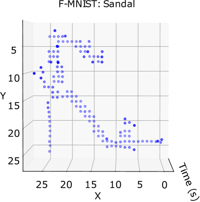
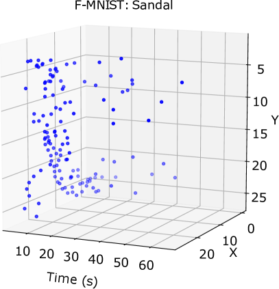
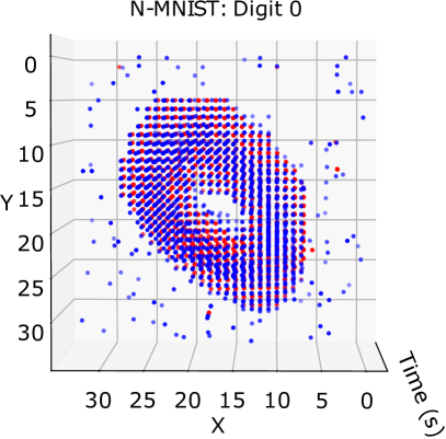
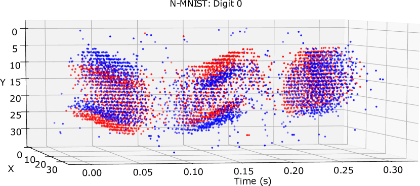
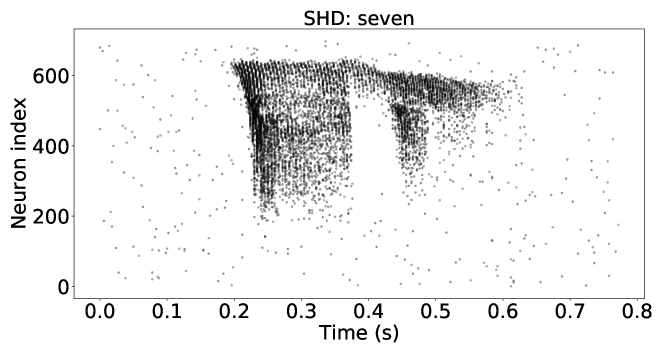
We evaluated the correctness and improved efficiency of the proposed sparse backpropagation algorithm on real data of varying difficulty and increasing spatio-temporal complexity. Firstly, the Fashion-MNIST dataset (F-MNIST) [44] is an image dataset that has been previously used on SNNs by converting each pixel analogue value to spike latencies such that a higher intensity results in an earlier spike [39][38]. Importantly, each input neuron can only spike at most once thus resulting in a simple spatio-temporal complexity and very sparse coding. Secondly, we used the Neuromorphic-MNIST (N-MNIST) [45] dataset where spikes are generated by presenting images of the MNIST dataset to a neuromorphic vision sensor. This dataset presents a higher temporal complexity and lower sparsity than the F-MNIST as each neuron can spike several times and there is noise from the recording device. Finally, we worked on the Spiking Heidelberg Dataset (SHD) [46]). This is a highly complex dataset that was generated by converting spoken digits into spike times by using a detailed model of auditory bushy cells in the cochlear nucleus. This results in a very high spatio-temporal complexity and lowest input sparsity. A visualisation of samples of each dataset can be found in the supplementary materials. These datasets cover the most relevant applications of neuromorphic systems. Namely, artificially encoding a dataset into spikes (Fashion-MNIST), reading spikes from a neuromorphic sensor such as a DVS camera (N-MNIST) and encoding complex temporally-varying data into spikes (SHD).

We run all experiments on three-layer fully connected network as in Fig. 1, where the last layer (readout) has an infinite threshold. Both spiking layers in the middle have the same number of neurons. We used $g(V):=1/(\beta|V-V_{th}|+1)^{2}$ for the surrogate gradient as in [38]. See Appendix E for all training details. We implemented the sparse gradient computation as a Pytorch CUDA extension [49].

3.1 Spiking neurons are inactive most of the time resulting in higher energy efficiency

One of the most determining factors of the success of our sparse gradient descent resides on the level of sparsity that we can expect and, consequently, the proportion of active neurons we have in each layer. We measure the percentage of active neurons on each batch as training progresses for each dataset. This can be computed as

$$\text{Activity}=100\times\frac{\text{\# of active neurons}}{BTN}$$ (13)

where $B$ is the batch size $T$ is the total number of time steps and $N$ the number of neurons in the layer and the number of active neurons is obtained according to (7). This is an empirical way of measuring the coefficient $\rho_{l}$ introduced earlier.

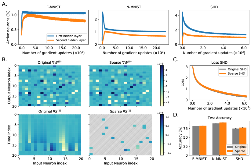
Figure 3A shows the activity on each dataset. As expected, the level of activity is correlated with the sparseness of the inputs with the lowest one being on the F-MNIST and the larger in the SHD dataset. Remarkably however, the activity on average is never above $2\%$ on average in any dataset and it is as low as $1.06\%$ in the F-MNIST dataset. This means that on average we will never have to compute more than $2\%$ of the factors in $\nabla W$ and $2\%$ of the values of $\nabla S$. This can be visualised in the bottom row of Fig. 3B.

These coefficients give us a theoretical upper bound to the amount of energy that can be saved if this sparse backpropagation rule was implemented in specialised hardware which only performed the required sums and products. This is summarised in Table 2.

Table 2: Theoretical upper bound to energy saved in hidden layers.

	Mean activity	Mean activity	Energy saved	Energy saved
	layer 1 (%)	layer 2 (%)	in $\nabla W$ (%)	in $\nabla S$ (%)
F-MNIST	1.06	0.87	99.13	98.94
N-MNIST	1.12	0.77	99.23	98.88
SHD	1.70	1.09	98.91	98.30

Importantly, in dense backpropagation methods the temporal dimension of datasets and models is necessarily limited to a maximum of $\sim\!2000$ since gradients must be computed at all steps [46, 39]. This means that a lot of negligible gradients are computed. However, our method adapts to the level of activity of the network and only computes non-negligible gradients. This cost-prohibitive reality was evidenced when we attempted to run these experiments in smaller GPUs leading to running out of memory when using dense methods but not on ours (see F.8). Thus, sparse spiking backpropagation allows to train data that runs for longer periods of time without requiring a more powerful hardware.

Figure 3: Sparse backpropagation learns at high levels of sparsity. All figures except B are a 5 sample average. Standard error in the mean is displayed (although too small to be easily visualised). A. Percentage of active neurons during training as a fraction of total tensor size ($B\!\times\!T\!\times\!N$) with $N\!=\!200$ neurons for each dataset. B. Visualisation of the weight and spike gradients on the SHD dataset. We show zero value in hatched grey. Note how both $\nabla W^{(0)}$ are nearly identical in despite being computed using a small fraction of the values of $\nabla S^{(1)}$ in the sparse case. C. Loss evolution on the SHD dataset using both algorithms. D. Final test accuracy on all datasets using both methods.

3.2 Sparse backpropagation training approximates the gradient very well

We test that our sparse learning rule performs on par with the standard surrogate gradient descent. Figure 3B shows a visualisation of the weight (first row) and spike gradients (second row). Note how most of the values of $\nabla S^{(1)}$ were not computed and yet $\nabla W^{(1)}$ is nearly identical to the original gradient. This is further confirmed in Figures 3C and 3D where the loss on the SHD dataset is practically identical with both methods (the loss for the other datasets can be found in Appendix F) and the test accuracy is practically identical (albeit slightly better) in the sparse case (F-MNIST: $82.2\%$, N-MNIST: $92.7\%$, SHD: $77.5\%$). These accuracies are on par to those obtained with similar networks on these datasets (F-MNIST: $80.1\%$, N-MNIST: $97.4\%$, SHD: $71.7\%$) [46, 38, 39]. These results show that sparse spiking backpropagation gives practically identical results to the original backpropagation but at much lower computational cost.

3.3 Sparse training is faster and less memory intensive

We now measure the time it takes the forward and the backward propagation of the second layer of the network during training as well as the peak GPU memory used. We choose this layer because it needs to compute both $\nabla W^{(1)}$ and $\nabla S^{(1)}$ (note that the first layer only needs to compute $\nabla W^{(0)}$). A performance improvement in this layer translates to an improvement in all subsequent layers inn a deeper network. We compute the backward speedup as the ratio of the original backpropagation time and the sparse backpropagation time. We compute the memory saved as

$$\text{Memory saved}=100\times\frac{\text{memory\_original}-\text{memory\_sparse}}{\text{memory\_original}}$$ (14)

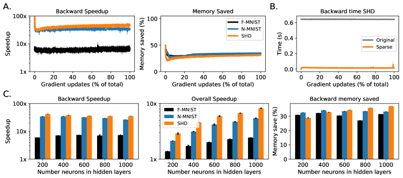
Figure 4A shows the speedup and memory saved on a $200$ neuron hidden layer (both hidden layers). Backpropagation time is faster by $40$x and GPU memory is reduced by $35\%$. To put this speedup into perspective Figure 4B shows the time taken for backpropagating the second layer in the original case (about $640$ms) and the sparse case (about $17$ms). It also shows that the time taken for backpropagating is nearly constant during training as it could be expected after studying the network activity in Fig. 3A.

We also tested how robust is this implementation for a varying number of hidden neurons (in both layers). We increase the number of neurons up to $1000$ which is similar to the maximum number of hidden units used in previous work [46] and it is also the point at which the original backpropagation method starts to run out of memory. Here we also show the overall speedup defined as the ratio between the sum of forward and backward times of the original over the sparse backpropagation. The results shown in Fig. 4C show that the backward speedup and memory saved remain constant as we increase the number of hidden neurons but the overall speedup increases substantially. Given that the forward time is the same for both methods (see Appendix F) this shows that as we increase the number of neurons, the backward time takes most of the computation and thus the sparse backpropagation becomes more important.

We also note that these results vary depending on the GPU used, Figure 4 was obtained from running on an RTX6000 GPU. We also run this on smaller GPUs (GTX1060 and GTX1080Ti) and found that the improvement is even better reaching up to a $70$x faster backward pass on N-MNIST and SHD. These results can found in Appendix F. Our results show that our method speeds up backward execution between one and two orders of magnitude, meaning that to a first approximation we would expect it reduce energy usage by the same factor since GPUs continue to use 30-50% of their peak power even when idle [50].

Figure 4: Speedup and memory improvement when using sparse gradient backpropagation. All figures are a 5 sample average and its standard error in the mean is also displayed. A. Backward speedup and memory saved in the second hidden layer for all three datasets when using sparse gradient descent with $200$ hidden neurons. B. Time spent in computing the backward pass in the second hidden layer consisting of $200$ neurons when using regular gradient descent and sparse gradient descent. C. Backward speed and memory saved in the second hidden layer as we increase the number of hidden neurons in all hidden layers. We included the overall speedup which takes into consideration both the forward and backward times spent in the second layer.

3.4 Training deeper and more complex architectures

We show that our gradient approximation can successfully train deeper networks by training a 6-layer fully connected network (5 hidden plus readout all with 300 neurons) on Fashion-MNIST. We measured the performance of the 5 hidden layers and achieve a $15$x backward speedup when using 1080-Ti GPU (better than the $10$x speedup under these conditions with only 2 hidden layers as shown in Appendix F.8) and $25\%$ memory saved while achieving a $82.7\%$ testing accuracy (slightly better than with 2 layers at $81.5\%$). The results are consistent with our previous findings and show that the gradient is not loss in deeper architectures.

We also run a experiment with a convolutional and pooling layers on the Fashion-MNIST dataset obtaining a test accuracy of $86.7\%$ when using our spike gradient approximation and $86.9\%$ with the original gradients. We do not report speedup or memory improvements in this network as developing a sparse convolutional CUDA kernel is out of the scope of our work but we simply ran a dense implementation with clamped gradients. This proves that our gradient approximation is able to train on more complex architectures although it still remains to be shown whether efficient sparse operators can be implemented for this purpose. See Appendix E for training details.

3.5 Sparsity-Accuracy trade-off

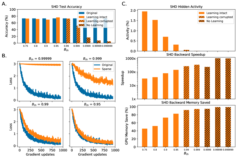
We trained the SHD dataset on the original 2-layer fully connected network with $400$ neurons in each hidden layer and varied the backpropagation threshold $B_{th}$. We found that the training is very robust to even extreme values of $B_{th}$. The loss and accuracy remains unchanged even when setting $B_{th}=0.95$ (see 5A and 5B) achieving a nearly $150$x speedup and $85\%$ memory improvement as shown in 5C. We also inspected the levels of activity while varying $B_{th}$ and we found that there are enough active neuron to propagate the gradient effectively. As $B_{th}$ gets closer to $1$ the number of active neurons decreases rapidly until there are no gradients to propagate.

Figure 5: Impact of varying the backpropagation threshold $B_{th}$ on the SHD dataset. A. Final test accuracy on the SHD dataset as $B_{th}$ increases. B. Loss evolution on the SHD dataset for different $B_{th}$. C. Hidden activity, backward speedup and backward memory saved as $B_{th}$ increases.

4 Discussion

Recent interest in neuromorphic computing has lead to energy efficient emulation of SNNs in specialised hardware. Most of these systems only support working with fixed network parameters thus requiring an external processor to train. Efforts to include training within the neuromorphic system usually rely on local learning rules which do not guarantee state-of-the-art performance. Thus, training on these systems requires error backpropagation on von-Neumann processors instead of taking advantage of the physics of the neuromorphic substrate [51, 52].

We have developed a sparse backpropagation algorithm for SNNs that achieves the same performance as standard dense backpropagation at a much reduced computational and memory cost. To the best of our knowledge this is the first backpropagation method that leverages the sparse nature of spikes in training and tackles the main performance bottleneck in neuromorphic training. Moreover, while we have used dense all-to-all connectivity between layers, our algorithm is compatible with other SNNs techniques that aim for a sparser connectivity such as synaptic pruning [53].

By constraining backpropagation to active neurons exclusively, we reduce the number of nodes and edges in the backward computation graph to a point where over $98$% of the operations required to compute the gradients can be skipped. This results in a much faster backpropagation time, lower memory requirement and less energy consumption on GPU hardware while not affecting the testing accuracy. This is possible because the surrogate gradient used to approximate the derivative of the spiking function is larger when the membrane potential is closer to the threshold resulting in most of the gradient being concentrated on active neurons. Previous work has used, to a lesser extent, similar ideas. Esser et al. [18] used a surrogate gradient function which effectively resulted in about one third the neurons backpropagating a zero gradient. Later, Pozzi, et al. [54] developed a learning rule where only the weights of neurons directly affecting the activity of the selected output class are updated, however, the trial and error nature of the learning procedure resulted in up to $3.5$x slower training.

However, due to the lack of efficient sparse operators in most auto-differentiation platforms, every layer type requires to develop its own sparse CUDA kernel in order to be competitive with current heavily optimised libraries. In our work, we concentrated on implementing and testing this in spiking fully connected layers and we managed to show that sparse backpropagation is a lot faster and uses less memory. Developing these sparse kernels is not trivial and we are aware that having to do so for each layer is an important limitation of our work. This is no surprise since for now there is few reasons to believe that sparse tensor operations will significantly accelerate neural network performance. Our work aims to challenge this view and motivate the adoption of efficient sparse routines by showing for the first time that sparse BPTT can be faster without losing accuracy.

We implemented and tested our method on real data on fully connected SNNs and simulated it in convolutional SNNs. The same method can be extended to any SNN topology as long as the neurons use a threshold activation function and the input is spiking data. However, due to the lack of efficient sparse operators in most auto-differentiation platforms, every layer type requires to develop its own sparse CUDA kernel in order to be competitive with current heavily optimised libraries. Developing these sparse kernels is not trivial and we are aware that having to do so for each layer is an important limitation of our work. This is no surprise since for now there is few reasons to believe that sparse tensor operations will significantly accelerate neural network performance. Our work aims to challenge this view and motivate the adoption of efficient sparse routines by showing for the first time that sparse spiking BPTT can be faster while achieving the same accuracy as its dense counterpart. Nevertheless, ideally, a dynamic backward graph should be generated each time the backward pass needs to be computed and consequently a GPU may not be the best processing unit for this task. A specialised neuromorphic implementation or an FPGA may be more suited to carry out the gradient computation task as this graph changes every batch update. Additionally, while we have reduced the number of operations required for training several times, we have only achieved up to a $85\%$ memory reduction thus, memory requirements remains an important bottleneck.

In summary, our sparse backpropagation algorithm for spiking neural networks tackles the main bottleneck in training SNNs and opens the possibility of a fast, energy and memory efficient end-to-end training on spiking neural networks which will benefit neuromorphic training and computational neuroscience research. Sparse spike backpropagation is a necessary step towards a fully efficient on-chip training which will be ultimately required to achieve the full potential of neuromorphic computing.

Sparse Spiking Gradient Descent: Supplementary Materials

Appendix A Proof of Proposition 1

Proposition 1.

We can use a recurrent relation to compute $\delta_{j}[t]$ given by

$${\color[rgb]{0.44,0.19,0.63}\delta_{j}[t]}=\begin{cases}\alpha^{n}{\color[rgb]{0.44,0.19,0.63}\delta_{j}[t+n]},\quad&\text{ if }{\color[rgb]{1,0,0}\frac{dS_{j}[k]}{dV_{j}[k]}}\!=\!0,\text{ for }t\!+\!1\!\leq\!k\!\leq\!t\!+\!n\\ {\color[rgb]{0,0.69,0.31}\nabla S_{j}[t\!+\!1]}{\color[rgb]{1,0,0}\frac{dS_{j}[t+1]}{dV_{j}[t+1]}}\!+\!\alpha^{n}{\color[rgb]{0.44,0.19,0.63}\delta_{j}[t\!+\!n]},\quad&\text{ if }{\color[rgb]{1,0,0}\frac{dS_{j}[k]}{dV_{j}[k]}}\!=\!0,\text{ for }t\!+\!1\!<\!k\!\leq\!t\!+\!n,{\color[rgb]{1,0,0}\frac{dS_{j}[t+1]}{dV_{j}[t+1]}}\!\neq\!0\\ \end{cases}$$ (15)

Proof.

The proof follows directly from the definition of $\delta_{j}[t]$.

For the first case we have

$$\delta_{j}[t] =\sum_{k>t}\nabla S_{j}[k]\frac{dS_{j}[k]}{dV_{j}[k]}\alpha^{k-t-1}$$

$$=\nabla S_{j}[t+1]\frac{dS_{j}[t+1]}{dV_{j}[t+1]}\alpha^{0}+S_{j}[t+2]\frac{dS_{j}[t+2]}{dV_{j}[t+2]}\alpha^{1}+\ldots+\nabla S_{j}[t+n]\frac{dS_{j}[t+n]}{dV_{j}[t+n]}\alpha^{n-1}$$

$$+\nabla S_{j}[t+n+1]\frac{dS_{j}[t+n+1]}{dV_{j}[t+n+1]}\alpha^{n}+\ldots$$

$$=\nabla S_{j}[t+1]\frac{dS_{j}[t+1]}{dV_{j}[t+1]}\alpha^{0}+S_{j}[t+2]\frac{dS_{j}[t+2]}{dV_{j}[t+2]}\alpha^{1}+\ldots+\nabla S_{j}[t+n]\frac{dS_{j}[t+n]}{dV_{j}[t+n]}\alpha^{n-1}$$

$$+\sum_{k>t+n}\nabla S_{j}[k]\frac{dS_{j}[k]}{dV_{j}[k]}\alpha^{k-t-1}$$

$$=\alpha^{n}\sum_{k>t+n}\nabla S_{j}[k]\frac{dS_{j}[k]}{dV_{j}[k]}\alpha^{k-(t+n)-1}$$

$$=\alpha^{n}\delta_{j}[t+n]$$

where the penultimate equality holds from the condition $\frac{dS_{j}[k]}{dV_{j}[k]}\!=\!0,\text{ for }t\!+\!1\!\leq\!k\!\leq\!t\!+\!n$

The proof of the second case is identical except that now the term $\nabla S_{j}[t+1]\frac{dS_{j}[t+1]}{dV_{j}[t+1]}$ will be non-zero.

Appendix B Complexity analysis

For clarity, we consider that all layers have the same number $N$ of neurons. The weight gradient is given by

$$\nabla W^{(l)}_{ij}=\sum_{t}{\color[rgb]{0,0.69,0.31}\nabla S_{j}^{(l+1)}[t]}{\color[rgb]{1,0,0}\frac{dS_{j}^{(l+1)}[t]}{dV_{j}^{(l+1)}[t]}}{\color[rgb]{0,0.44,0.75}\left(\sum_{k<t}\alpha^{t-k-1}S_{i}^{(l)}[t]\right)}$$

Since the trace $\left({\color[rgb]{0,0.44,0.75}\sum_{k<t}\alpha^{t-k-1}S_{i}^{(l)}[t]}\right)$ has been compated in the forward pass, then computing $\nabla W^{(l)}_{ij}$ requires doing a total of $T$ products and $T\!-\!1$ sums per element in $W$ per batch. Thus resulting in $O(BTN^{2})$ products and $O(BTN^{2})$ sums. In the sparse case instead of $T$ we have on average $\rho_{l+1}T$ products and $\rho_{l+1}(T\!-\!1)$ sums resulting in a total of $O(\rho_{l+1}BTN^{2})$ products and $O(\rho_{l+1}BTN^{2})$ sums.

The spikes gradient is given by

$${\color[rgb]{0,0.69,0.31}\nabla S^{(l)}_{i}[t]} =\sum_{j}W_{ij}\left(\vphantom{\sum_{j}W_{ij}\frac{dS_{j}^{(l+1)}[t]}{dV_{j}^{(l+1)}[t]}}\right.\sum_{k>t}{\color[rgb]{0,0.69,0.31}\nabla S_{j}^{(l+1)}[t]}{\color[rgb]{1,0,0}\frac{dS_{j}^{(l+1)}[t]}{dV_{j}^{(l+1)}[t]}}\alpha^{k-t-1}\left.\vphantom{\sum_{j}W_{ij}\frac{dS_{j}^{(l+1)}[t]}{dV_{j}^{(l+1)}[t]}}\right)$$

$$=\sum_{j}W_{ij}{\color[rgb]{0.44,0.19,0.63}\delta^{(l+1)}_{j}[t]}$$

This gradient is obtained by doing the matrix product between $W\in\mathbb{R}^{N\times N}$ and ${\color[rgb]{0.44,0.19,0.63}\delta^{(l+1)}}\in\mathbb{R}^{N\times T}$ per batch. This gives a total of $O(BN^{2}T)$ products and sums. In the sparse case we only need to compute a fraction $\rho_{l}$ of the entries in ${\color[rgb]{0,0.69,0.31}\nabla S^{(l)}}$ thus a total of $O(\rho_{l}BN^{2}T)$ products and sums.

There are two main ways of computing ${\color[rgb]{0.44,0.19,0.63}\delta^{(l+1)}}$. The naive way requires doing $O(NT^{2})$ products and $O(NT^{2})$ sums by computing all values with $k>t$ for a given $t$ every time. Alternatively, we can use memoisation to store all values already computed resulting in just $O(NT)$ products and $O(NT)$ sums per batch. Thus resulting in $O(BNT)$ products and sums. In the sparse case, the worst case scenario is when the active times of layers $l$ and $l\!+\!1$ are completely disjoint as we show in Appendix C. Meaning we have to compute $O((\rho_{l}\!+\!\rho_{l+1})BNT^{2})$ products and sums without memoisation or $O((\rho_{l}\!+\!\rho_{l+1})BNT)$ with memoisation.

Overall we get that if we do not use memoisation for computing ${\color[rgb]{0,0.69,0.31}\nabla S^{(}l)}$ then we do $O(B(NT^{2}+N^{2}T))$ sums and products and $O(B((\rho_{l+1}\!+\!\rho_{l})NT^{2}+\rho_{l+1}N^{2}T)$ in the sparse case. With memoisation we do $O(BN^{2}T)$ and $O(\rho_{l+1}BN^{2}T)$ in the sparse case.

Appendix C Visualisation of $\delta_{j}[t]$ computation

Given a presynaptic neuron $i$ and postsynaptic neuron $j$ we need to compute the gradient

$${\color[rgb]{0,0.69,0.31}\nabla S_{i}[t]} =\sum_{j}W_{ij}\left(\vphantom{\sum_{j}W_{ij}\frac{dS_{j}[t]}{dV_{j}[t]}}\right.\sum_{k>t}{\color[rgb]{0,0.69,0.31}\nabla S_{j}[t]}{\color[rgb]{1,0,0}\frac{dS_{j}[t]}{dV_{j}[t]}}\alpha^{k-t-1}\left.\vphantom{\sum_{j}W_{ij}\frac{dS_{j}[t]}{dV_{j}[t]}}\right)$$

$$=\sum_{j}W_{ij}{\color[rgb]{0.44,0.19,0.63}\delta_{j}[t]}$$

We first note that ${\color[rgb]{0,0.69,0.31}\nabla S_{i}[t]}$ is always multiplied by $\frac{dS_{i}[t]}{dV_{i}[t]}$ either in the weight gradient equation (5) or in the spike gradient equation (6). Thus, we only need ${\color[rgb]{0,0.69,0.31}\nabla S_{i}[t]}$ at those times at which $\frac{dS_{i}[t]}{dV_{j}[t]}\!\neq\!0$.

Secondly, according to Proposition 1 ${\color[rgb]{0.44,0.19,0.63}\delta_{j}[t]}$ is only modified beyond an attenuation factor of $\alpha^{n}$ at those times when ${\color[rgb]{0,0.69,0.31}\frac{dS_{j}[t]}{dV_{j}[t]}\!\neq\!0}$.

We define

$${\color[rgb]{0,0.69,0.31}t_{i}} =\{t:\frac{dS_{i}[t]}{dV_{i}[t]}\neq 0\}\quad\text{The times we \emph{need} to compute the gradient of the presynaptic neuron $i$}$$

$${\color[rgb]{1,0,0}t_{j}} =\{t:{\color[rgb]{1,0,0}\frac{dS_{j}[t]}{dV_{j}[t]}}\neq 0\}\quad\text{The times that affect $\delta_{j}$ beyond $\alpha^{n}$ attenuation}$$

Both sets of times are known by the time we compute the gradients since they are simply the times at which neurons $i$ and $j$ were active.

The following example shows how the computation of $\delta_{j}[t]$ would take place using Proposition 1. We note that we only need to write the result in global memory at times ${\color[rgb]{0,0.69,0.31}t_{i}}$. Consequently, once we have all ${\color[rgb]{0,0.69,0.31}t_{i}}$ we can simply stop the computation

$${\color[rgb]{0.44,0.19,0.63}\delta_{j}[7]} ={\color[rgb]{1,0,0}\frac{dS_{j}[8]}{dV_{j}[8]}}$$ Compute

$${\color[rgb]{0.44,0.19,0.63}\delta_{j}[6]} =\alpha{\color[rgb]{0.44,0.19,0.63}\delta_{j}[7]}$$ Compute and write

$${\color[rgb]{0.44,0.19,0.63}\delta_{j}[5]} ={\color[rgb]{1,0,0}\frac{dS_{j}[6]}{dV_{j}[6]}}+\alpha{\color[rgb]{0.44,0.19,0.63}\delta_{j}[6]}$$ Compute and write

$${\color[rgb]{0.44,0.19,0.63}\delta_{j}[3]} =\alpha^{2}{\color[rgb]{0.44,0.19,0.63}\delta_{j}[5]}$$ Compute and write

$${\color[rgb]{.5,.5,.5}\delta_{j}[2]} ={\color[rgb]{.5,.5,.5}\frac{dS_{j}[3]}{dV_{j}[3]}+\alpha\delta_{j}[3]}$$ Not required

$${\color[rgb]{.5,.5,.5}\delta_{j}[0]} ={\color[rgb]{.5,.5,.5}\frac{dS_{j}[1]}{dV_{j}[1]}+\alpha^{2}\delta_{j}[2]}$$ Not required

Thus, in the worse case scenario where sets ${\color[rgb]{0,0.69,0.31}t_{i}}$ and ${\color[rgb]{1,0,0}t_{j}}$ are disjoint instead of doing $T$ updates we only do $|t_{i}|+|t_{j}|$ updates.

Appendix D Visualisation of input data

Visualisation of several of one sample per dataset to provide and intuitive idea of the level of sparsity of the data.

Figure 6: Visulization of a sample of the Fashion-MNIST dataset converted into spike times. Left: Front view. Right: Side view

Figure 7: Visulization of a sample of the Neuromorphic-MNIST dataset. Top: Front view. Bottom: Side view

Figure 8: Visulization of a sample of the Spiking Heidelberg Digits dataset.

Appendix E Training details

E.1 Conversion of Fashion-MNIST to spike latencies

We convert the normalised analog grayscale pixel values $x_{i}$ of the Fashion-MNIST samples [44] to spike times in a similar way to that used in [38]. Specifically, we convert the normalised intensities into spike times following

$$T(x)=\begin{cases}\tau_{\text{eff}}\log{\left(\frac{x}{x-\theta}\right)},\quad x>\theta\\ \infty,\quad\text{otherwise}\end{cases}$$

E.2 Spiking neuron model

We use the simplified Leaky Integrate and Fire model which is a variation on the standard Leaky Integrate and Fire model in which spikes are directly integrated in the membrane without being filtered by beforehand. The membrane potential evolves according to

$$\tau\frac{dV^{(l+1)}_{j}(t)}{dt}=-(V^{(l+1)}_{j}(t)-V_{rest})+\tau\sum_{i}S^{(l)}_{i}[t]W^{(l)}_{ij}$$ (16)

The membrane potential resets to $V_{r}$ as soon as it reaches a threshold $V_{th}$. The model keeps the main features of a spiking model, namely, a membrane potential that varies according to the incoming input spikes and synaptic weights, a leaky component that draws the potential towards $V_{rest}$ and spiking and resetting mechanisms.

We use a discretised version of the model as in Equation (2) that we repeat here

$$V^{(l\!+\!1)}_{j}[t\!+\!1]=-\alpha(V^{(l+1)}_{j}[t]-V_{rest})+\sum_{i}S^{(l)}_{i}[t]W^{(l)}_{ij}-(V_{th}-V_{r})S^{(l\!+\!1)}_{j}[t]$$ (17)

where we define $\alpha=exp(-\Delta t/\tau)$. Spiking then takes place by applying $f(\cdot)$ on the membrane potential

$$S^{(l\!+\!1)}_{j}[t\!+\!1]=f(V^{(l\!+\!1)}_{j}[t\!+\!1])$$ (18)

which is defined as a unit step function centered at the threshold $V_{th}$

$$f(v)=\begin{cases}1,&\quad v>V_{th}\\ 0,&\quad\text{otherwise}\end{cases}$$ (19)

Thus, given an input spikes tensor $S^{(l)}\!\in\!\{0,1\}^{B\!\times\!T\!\times\!N^{(l)}}$ ($B$ being the batch size $T$ number of time steps and $N^{(l)}$ number of neurons in layer $l$) and weights $W^{(l)}\!\in\!\mathbb{R}^{N^{(l)}\!\times\!N^{(l\!+\!1)}}$ we obtain the output spikes $S^{(l\!+\!1)}\!\in\!\{0,1\}^{B\!\times\!T\!\times\!N^{(l\!+\!1)}}$ by applying (17), (18), (19).

E.3 Network and weight initialisation

All layers are feed-forward fully connected in all experiments unless otherwise specified. The weights were sampled from a uniform distribution $\mathcal{U}(-\sqrt{N},\sqrt{N})$ where $N$ is the number of input connections to the layer. In all experiments we have an input layer, two hidden layers with the same number of neurons and a readout layer with as many neurons as output classes for the given dataset. The readout layer neurons are identical to the hidden layers except in the firing threshold which we set to infinity.

In the convolutional layer experiment, the first layer was a convolutional spiking layer with $64$ filters, kernel size of $3$ and stride of $1$, followed by a max pool layer with kernel size of $2$ and then flattened into a linear layer of $12544$ inputs and 10 outputs.

E.4 Supervised and regularisation losses

We have a loss composed of three terms: cross entropy loss, higher activity regularisation and lower activity regularisation. The cross entropy loss is defined as

$$\mathcal{L}^{cross}=\frac{1}{B}\sum_{b=1}^{B}\sum_{c=1}^{C}y_{b,c}\log(p_{b,c})$$

With $y_{b,c}\!\in\!\{0,1\}^{C}$ being a one hot target vector for batch sample $b$ given a total batch size $B$ and a total number of classes $C$. The probabilities $p_{b,c}$ are obtained using the Softmax function

$$p_{b,c}=\frac{e^{a_{b,c}}}{\sum_{c=1}^{C}e^{a_{b,c}}}$$

Here, the logits $a_{b,c}\!\in\!\mathbb{R}^{B\!\times\!C}$ are obtained by taking the max over the time dimension on the readout layer membrane potential $a_{b,c}=\max_{t}V^{(L\!-\!1)}_{b,c}[t]$. For the SHD dataset we used $a_{b,c}=\sum_{t}V^{(L\!-\!1)}_{b,c}[t]$

We also use two regularisation terms to constrain the spiking activity. These terms have been shown to not degrade the network performance [38]. First, we use a lower activity penalty to promote activity in the hidden layers.

$$\mathcal{L}^{low}_{b}=-\frac{\lambda^{low}}{N^{(l)}}\sum_{i}^{N^{(l)}}\left(\max(0,\nu^{low}-\zeta_{b,i}^{(l)})\right)^{2}$$

Here $\zeta_{b,i}^{(l)}=\sum_{t}S_{b,i}^{l}[t]$ is the spike count of neuron $i$ in layer $l$ and batch sample $b$.

Secondly, the upper activity loss is added to prevent neurons to spike too often.

$$\mathcal{L}^{up}_{b}=-\lambda^{up}\max\left(0,\frac{1}{N^{(l)}}\sum_{i}^{N^{(l)}}\zeta_{b,i}^{(l)}-\nu^{up}\right)$$

Finally the overall loss is obtained

$$\mathcal{L}=\mathcal{L}^{cross}+\frac{1}{B}\sum_{b\!=\!1}^{B}\left(\mathcal{L}^{low}_{b}+\mathcal{L}^{up}_{b}\right)$$

E.5 Surrogate gradient

We use the following function as the surrogate derivate of the firing function defined in (19).

$$\frac{df(x)}{dx}=g(x)=\frac{1}{(\beta|x-V_{th}|+1)^{2}}$$

In the sparse case we use

$$\frac{df(x)}{dx}=\begin{cases}g(x),\quad&\text{if }|x-V_{th}|<B_{th}\\ 0,\quad&\text{otherwise}\\ \end{cases}$$ (20)

E.6 Parameters

Here we summarise all parameters used in each dataset.

	F-MNIST	N-MNIST	SHD
Number of Input Neurons	$784$	$1156$	$700$
Number of Hidden	$200$	$200$	$200$
Number of classes	$10$	$10$	$20$
Number epochs	$100$	$100$	$200$
B	$256$	$256$	$256$
T	$100$	$300$	$500$
$\Delta t$	$1$ms	$1$ms	$2$ms
$\tau$ hidden	$10$ms	$10$ms	$10$ms
$\tau$ readout	$10$ms	$10$ms	$20$ms
$\tau_{\text{eff}}$	$20$ms	N/A	N/A
$\theta$	$0.2$	N/A	N/A
$V_{r}$	$0$	$0$	$0$
$V_{rest}$	$0$	$0$	$0$
$V_{th}$	$1$	$1$	$1$
$B_{th}$	$0.2$	$0.2$	$0.2$
$\beta$	$100$	$100$	$100$
Optimiser	Adam	Adam	Adam
Learning Rate	$0.0002$	$0.0002$	$0.001$
Betas	$(0.9,0.999)$	$(0.9,0.999)$	$(0.9,0.999)$
$\lambda^{(low)}$	$100$	$100$	$100$
$\nu^{(low)}$	$0.001$	$0.001$	$0.001$
$\lambda^{(up)}$	$0.06$	$0.06$	$0.06$
$\nu^{(up)}$	$1$	$1$	$10$

Table 3: Network and training parameters

Appendix F Other results

F.1 Average activity for varying number of hidden neurons

Figure 9: Average percentage of active neurons during training for each dataset and varying number of neurons (5 samples)

F.2 Loss evolution for all datasets

Figure 10: Loss for each dataset when using 200 hidden neurons (5 samples)

F.3 Forward times

Figure 11: Forward time for each dataset when using 200 hidden neurons (5 samples)

Figure 12: Average forward time for each dataset and varying number of neurons (5 samples)

F.4 Backward times

Figure 13: Backward time for each dataset when using 200 hidden neurons (5 samples)

Figure 14: Average backward time for each dataset and varying number of neurons (5 samples)

F.5 Forward memory

Figure 15: Forward memory for each dataset when using 200 hidden neurons (5 samples)

Figure 16: Average forward memory time for each dataset and varying number of neurons (5 samples)

F.6 Backward memory

Figure 17: Backward memory for each dataset when using 200 hidden neurons (5 samples)

Figure 18: Average backward memory for each dataset and varying number of neurons (5 samples)

F.7 Memory saved

Figure 19: Average memory saved according to (14) for each dataset and varying number of neurons (5 samples)

F.8 Results on different GPUs

Note that some entries are missing due to the GPU running out of memory.

Figure 20: Backward speedup, overall layer speedup and backward memory memory saved on an NVIDIA GeForce GTX 1060

Figure 21: Backward speedup, overall layer speedup and backward memory memory saved on an NVIDIA GeForce GTX 1080 Ti

Appendix G Results on 5 hidden layers network

Figure 22: Loss history and layer activities when training on Fashion-MNIST with 5 hidden layers with 300 neurons each

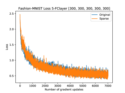
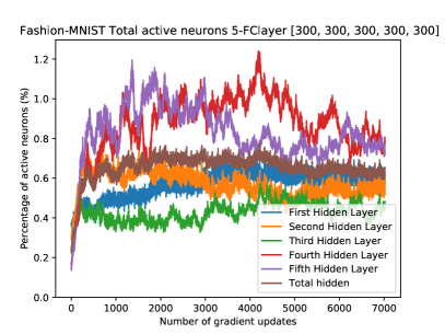
Appendix H Weight gradient difference and relative error

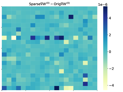
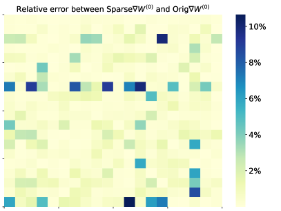
We show here the difference between the original weight gradient and that obtained from our method as well as its relative error. We like to note that the original gradient is not necessarily more accurate than the sparse one as surrogate gradient training results in approximated gradients. Thus, it is not a ground truth gradient and the real test is done by showing that our method achieves the same or better loss and testing accuracy.

Figure 23: Difference between the weight gradients displayed in 3. The maximum relative error between two individual weights is $10.6\%$

Checklist

1. For all authors…

   1. Do the main claims made in the abstract and introduction accurately reflect the paper’s contributions and scope? [Yes]

   2. Did you describe the limitations of your work? [Yes] See sections 2 and 4

   3. Did you discuss any potential negative societal impacts of your work? [N/A]

   4. Have you read the ethics review guidelines and ensured that your paper conforms to them? [Yes]

2. If you are including theoretical results…

   1. Did you state the full set of assumptions of all theoretical results? [Yes] See section 2 and Appendix A and B

   2. Did you include complete proofs of all theoretical results? [Yes] Section 2 and Appendix A and B

3. If you ran experiments…

   1. Did you include the code, data, and instructions needed to reproduce the main experimental results (either in the supplemental material or as a URL)? [Yes] The code has been included in the supplementary materials

   2. Did you specify all the training details (e.g., data splits, hyperparameters, how they were chosen)? [Yes] See Appendix E

   3. Did you report error bars (e.g., with respect to the random seed after running experiments multiple times)? [Yes] All experimental results include standard error in the mean over multiple trials. See section 3 and Appendix F

   4. Did you include the total amount of compute and the type of resources used (e.g., type of GPUs, internal cluster, or cloud provider)? [Yes] See section 3 and Appendix F

4. If you are using existing assets (e.g., code, data, models) or curating/releasing new assets…

   1. If your work uses existing assets, did you cite the creators? [Yes] The three datasets used have been cited

   2. Did you mention the license of the assets? [No] All three datasets are licensed either by Creative Commons Attribution-ShareAlike 4.0 license or MIT License. This will be included in the acknowledgements in the final version

   3. Did you include any new assets either in the supplemental material or as a URL? [Yes] The code used to run the experiments is included in the supplementary materials

   4. Did you discuss whether and how consent was obtained from people whose data you’re using/curating? [N/A]

   5. Did you discuss whether the data you are using/curating contains personally identifiable information or offensive content? [N/A]

5. If you used crowdsourcing or conducted research with human subjects…

   1. Did you include the full text of instructions given to participants and screenshots, if applicable? [N/A]

   2. Did you describe any potential participant risks, with links to Institutional Review Board (IRB) approvals, if applicable? [N/A]

   3. Did you include the estimated hourly wage paid to participants and the total amount spent on participant compensation? [N/A]

References

- [1] Yann LeCun, Yoshua Bengio, and Geoffrey Hinton. Deep learning. nature, 521(7553):436–444, 2015.
- [2] Geoffrey Hinton, Li Deng, Dong Yu, George E Dahl, Abdel-rahman Mohamed, Navdeep Jaitly, Andrew Senior, Vincent Vanhoucke, Patrick Nguyen, Tara N Sainath, et al. Deep neural networks for acoustic modeling in speech recognition: The shared views of four research groups. IEEE Signal processing magazine, 29(6):82–97, 2012.
- [3] Alex Krizhevsky, Ilya Sutskever, and Geoffrey E Hinton. Imagenet classification with deep convolutional neural networks. Advances in neural information processing systems, 25:1097–1105, 2012.
- [4] Zhengyan Zhang, Xu Han, Zhiyuan Liu, Xin Jiang, Maosong Sun, and Qun Liu. ERNIE: Enhanced language representation with informative entities. In Proceedings of the 57th Annual Meeting of the Association for Computational Linguistics, pages 1441–1451, Florence, Italy, July 2019. Association for Computational Linguistics.
- [5] Tom B Brown, Benjamin Mann, Nick Ryder, Melanie Subbiah, Jared Kaplan, Prafulla Dhariwal, Arvind Neelakantan, Pranav Shyam, Girish Sastry, Amanda Askell, et al. Language models are few-shot learners. arXiv preprint arXiv:2005.14165, 2020.
- [6] Volodymyr Mnih, Koray Kavukcuoglu, David Silver, Andrei A Rusu, Joel Veness, Marc G Bellemare, Alex Graves, Martin Riedmiller, Andreas K Fidjeland, Georg Ostrovski, et al. Human-level control through deep reinforcement learning. nature, 518(7540):529–533, 2015.
- [7] David Silver, Julian Schrittwieser, Karen Simonyan, Ioannis Antonoglou, Aja Huang, Arthur Guez, Thomas Hubert, Lucas Baker, Matthew Lai, Adrian Bolton, et al. Mastering the game of go without human knowledge. nature, 550(7676):354–359, 2017.
- [8] Oriol Vinyals, Igor Babuschkin, Wojciech M Czarnecki, Michaël Mathieu, Andrew Dudzik, Junyoung Chung, David H Choi, Richard Powell, Timo Ewalds, Petko Georgiev, et al. Grandmaster level in starcraft ii using multi-agent reinforcement learning. Nature, 575(7782):350–354, 2019.
- [9] Emma Strubell, Ananya Ganesh, and Andrew McCallum. Energy and policy considerations for deep learning in nlp. arXiv preprint arXiv:1906.02243, 2019.
- [10] Roy Schwartz, Jesse Dodge, Noah A. Smith, and Oren Etzioni. Green ai. Commun. ACM, 63(12):54–63, November 2020.
- [11] Jacob Hochstetler, Rahul Padidela, Qi Chen, Qing Yang, and Song Fu. Embedded deep learning for vehicular edge computing. In 2018 IEEE/ACM Symposium on Edge Computing (SEC), pages 341–343. IEEE, 2018.
- [12] Nicholas D Lane, Sourav Bhattacharya, Akhil Mathur, Petko Georgiev, Claudio Forlivesi, and Fahim Kawsar. Squeezing deep learning into mobile and embedded devices. IEEE Pervasive Computing, 16(3):82–88, 2017.
- [13] Jonathan W Mink, Robert J Blumenschine, and David B Adams. Ratio of central nervous system to body metabolism in vertebrates: its constancy and functional basis. American Journal of Physiology-Regulatory, Integrative and Comparative Physiology, 241(3):R203–R212, 1981.
- [14] Wulfram Gerstner, Werner M Kistler, Richard Naud, and Liam Paninski. Neuronal dynamics: From single neurons to networks and models of cognition. Cambridge University Press, 2014.
- [15] David Daniel Cox and Thomas Dean. Neural networks and neuroscience-inspired computer vision. Current Biology, 24(18):R921–R929, 2014.
- [16] Thomas Pfeil, Andreas Grübl, Sebastian Jeltsch, Eric Müller, Paul Müller, Mihai A Petrovici, Michael Schmuker, Daniel Brüderle, Johannes Schemmel, and Karlheinz Meier. Six networks on a universal neuromorphic computing substrate. Frontiers in neuroscience, 7:11, 2013.
- [17] Paul A Merolla, John V Arthur, Rodrigo Alvarez-Icaza, Andrew S Cassidy, Jun Sawada, Filipp Akopyan, Bryan L Jackson, Nabil Imam, Chen Guo, Yutaka Nakamura, et al. A million spiking-neuron integrated circuit with a scalable communication network and interface. Science, 345(6197):668–673, 2014.
- [18] Steven K Esser, Paul A Merolla, John V Arthur, Andrew S Cassidy, Rathinakumar Appuswamy, Alexander Andreopoulos, David J Berg, Jeffrey L McKinstry, Timothy Melano, Davis R Barch, et al. Convolutional networks for fast, energy-efficient neuromorphic computing. Proceedings of the national academy of sciences, 113(41):11441–11446, 2016.
- [19] Peter U Diehl, Guido Zarrella, Andrew Cassidy, Bruno U Pedroni, and Emre Neftci. Conversion of artificial recurrent neural networks to spiking neural networks for low-power neuromorphic hardware. In 2016 IEEE International Conference on Rebooting Computing (ICRC), pages 1–8. IEEE, 2016.
- [20] Misha Mahowald and Rodney Douglas. A silicon neuron. Nature, 354(6354):515–518, 1991.
- [21] Johannes Schemmel, Daniel Brüderle, Andreas Grübl, Matthias Hock, Karlheinz Meier, and Sebastian Millner. A wafer-scale neuromorphic hardware system for large-scale neural modeling. In 2010 IEEE International Symposium on Circuits and Systems (ISCAS), pages 1947–1950. IEEE, 2010.
- [22] Paul Merolla, John Arthur, Filipp Akopyan, Nabil Imam, Rajit Manohar, and Dharmendra S Modha. A digital neurosynaptic core using embedded crossbar memory with 45pj per spike in 45nm. In 2011 IEEE custom integrated circuits conference (CICC), pages 1–4. IEEE, 2011.
- [23] Saber Moradi and Giacomo Indiveri. An event-based neural network architecture with an asynchronous programmable synaptic memory. IEEE transactions on biomedical circuits and systems, 8(1):98–107, 2013.
- [24] Elisabetta Chicca, Fabio Stefanini, Chiara Bartolozzi, and Giacomo Indiveri. Neuromorphic electronic circuits for building autonomous cognitive systems. Proceedings of the IEEE, 102(9):1367–1388, 2014.
- [25] Ben Varkey Benjamin, Peiran Gao, Emmett McQuinn, Swadesh Choudhary, Anand R Chandrasekaran, Jean-Marie Bussat, Rodrigo Alvarez-Icaza, John V Arthur, Paul A Merolla, and Kwabena Boahen. Neurogrid: A mixed-analog-digital multichip system for large-scale neural simulations. Proceedings of the IEEE, 102(5):699–716, 2014.
- [26] Mike Davies, Narayan Srinivasa, Tsung-Han Lin, Gautham Chinya, Yongqiang Cao, Sri Harsha Choday, Georgios Dimou, Prasad Joshi, Nabil Imam, Shweta Jain, et al. Loihi: A neuromorphic manycore processor with on-chip learning. Ieee Micro, 38(1):82–99, 2018.
- [27] G Pedretti, V Milo, S Ambrogio, R Carboni, S Bianchi, A Calderoni, N Ramaswamy, AS Spinelli, and D Ielmini. Memristive neural network for on-line learning and tracking with brain-inspired spike timing dependent plasticity. Scientific reports, 7(1):1–10, 2017.
- [28] Chul-Heung Kim, Soochang Lee, Sung Yun Woo, Won-Mook Kang, Suhwan Lim, Jong-Ho Bae, Jaeha Kim, and Jong-Ho Lee. Demonstration of unsupervised learning with spike-timing-dependent plasticity using a tft-type nor flash memory array. IEEE Transactions on Electron Devices, 65(5):1774–1780, 2018.
- [29] Dongseok Kwon, Suhwan Lim, Jong-Ho Bae, Sung-Tae Lee, Hyeongsu Kim, Young-Tak Seo, Seongbin Oh, Jangsaeng Kim, Kyuho Yeom, Byung-Gook Park, et al. On-chip training spiking neural networks using approximated backpropagation with analog synaptic devices. Frontiers in neuroscience, 14:423, 2020.
- [30] Sebastian Schmitt, Johann Klähn, Guillaume Bellec, Andreas Grübl, Maurice Guettler, Andreas Hartel, Stephan Hartmann, Dan Husmann, Kai Husmann, Sebastian Jeltsch, et al. Neuromorphic hardware in the loop: Training a deep spiking network on the brainscales wafer-scale system. In 2017 international joint conference on neural networks (IJCNN), pages 2227–2234. IEEE, 2017.
- [31] Benjamin Cramer, Sebastian Billaudelle, Simeon Kanya, Aron Leibfried, Andreas Grübl, Vitali Karasenko, Christian Pehle, Korbinian Schreiber, Yannik Stradmann, Johannes Weis, et al. Training spiking multi-layer networks with surrogate gradients on an analog neuromorphic substrate. arXiv preprint arXiv:2006.07239, 2020.
- [32] Simon Davidson and Steve B Furber. Comparison of artificial and spiking neural networks on digital hardware. Frontiers in Neuroscience, 15, 2021.
- [33] Emre O. Neftci, Hesham Mostafa, and Friedemann Zenke. Surrogate gradient learning in spiking neural networks: Bringing the power of gradient-based optimization to spiking neural networks. IEEE Signal Processing Magazine, 36(6):51–63, 2019.
- [34] Timo C Wunderlich and Christian Pehle. Event-based backpropagation can compute exact gradients for spiking neural networks. Scientific Reports, 11(1):1–17, 2021.
- [35] Eric Hunsberger and Chris Eliasmith. Spiking deep networks with lif neurons. arXiv preprint arXiv:1510.08829, 2015.
- [36] Sumit Bam Shrestha and Garrick Orchard. Slayer: Spike layer error reassignment in time. In S. Bengio, H. Wallach, H. Larochelle, K. Grauman, N. Cesa-Bianchi, and R. Garnett, editors, Advances in Neural Information Processing Systems, volume 31. Curran Associates, Inc., 2018.
- [37] Stanisław Woźniak, Angeliki Pantazi, Thomas Bohnstingl, and Evangelos Eleftheriou. Deep learning incorporating biologically inspired neural dynamics and in-memory computing. Nature Machine Intelligence, 2(6):325–336, 2020.
- [38] Friedemann Zenke and Tim P Vogels. The remarkable robustness of surrogate gradient learning for instilling complex function in spiking neural networks. Neural Computation, 33(4):899–925, 2021.
- [39] Nicolas Perez-Nieves, Vincent CH Leung, Pier Luigi Dragotti, and Dan FM Goodman. Neural heterogeneity promotes robust learning. bioRxiv, pages 2020–12, 2021.
- [40] Lei Jimmy Ba Brendan Frey. Adaptive dropout for training deep neural networks. Proceeding NIPS, 13:3084–3092, 2013.
- [41] Guy Blanc and Steffen Rendle. Adaptive sampled softmax with kernel based sampling. In International Conference on Machine Learning, pages 590–599. PMLR, 2018.
- [42] Beidi Chen, Tharun Medini, James Farwell, Sameh Gobriel, Charlie Tai, and Anshumali Shrivastava. Slide: In defense of smart algorithms over hardware acceleration for large-scale deep learning systems. arXiv preprint arXiv:1903.03129, 2019.
- [43] Shabnam Daghaghi, Nicholas Meisburger, Mengnan Zhao, and Anshumali Shrivastava. Accelerating slide deep learning on modern cpus: Vectorization, quantizations, memory optimizations, and more. Proceedings of Machine Learning and Systems, 3, 2021.
- [44] Han Xiao, Kashif Rasul, and Roland Vollgraf. Fashion-mnist: a novel image dataset for benchmarking machine learning algorithms. arXiv preprint arXiv:1708.07747, 2017.
- [45] Garrick Orchard, Ajinkya Jayawant, Gregory K Cohen, and Nitish Thakor. Converting static image datasets to spiking neuromorphic datasets using saccades. Frontiers in neuroscience, 9:437, 2015.
- [46] Benjamin Cramer, Yannik Stradmann, Johannes Schemmel, and Friedemann Zenke. The heidelberg spiking data sets for the systematic evaluation of spiking neural networks. IEEE Transactions on Neural Networks and Learning Systems, 2020.
- [47] Wulfram Gerstner, Marco Lehmann, Vasiliki Liakoni, Dane Corneil, and Johanni Brea. Eligibility traces and plasticity on behavioral time scales: experimental support of neohebbian three-factor learning rules. Frontiers in neural circuits, 12:53, 2018.
- [48] Bojian Yin, Federico Corradi, and Sander M Bohté. Effective and efficient computation with multiple-timescale spiking recurrent neural networks. In International Conference on Neuromorphic Systems 2020, pages 1–8, 2020.
- [49] Adam Paszke, Sam Gross, Francisco Massa, Adam Lerer, James Bradbury, Gregory Chanan, Trevor Killeen, Zeming Lin, Natalia Gimelshein, Luca Antiga, Alban Desmaison, Andreas Kopf, Edward Yang, Zachary DeVito, Martin Raison, Alykhan Tejani, Sasank Chilamkurthy, Benoit Steiner, Lu Fang, Junjie Bai, and Soumith Chintala. Pytorch: An imperative style, high-performance deep learning library. In H. Wallach, H. Larochelle, A. Beygelzimer, F. d'Alché-Buc, E. Fox, and R. Garnett, editors, Advances in Neural Information Processing Systems 32, pages 8024–8035. Curran Associates, Inc., 2019.
- [50] James C Knight and Thomas Nowotny. Gpus outperform current hpc and neuromorphic solutions in terms of speed and energy when simulating a highly-connected cortical model. Frontiers in neuroscience, 12:941, 2018.
- [51] Giacomo Indiveri and Shih-Chii Liu. Memory and information processing in neuromorphic systems. Proceedings of the IEEE, 103(8):1379–1397, 2015.
- [52] Yigit Demirag, Filippo Moro, Thomas Dalgaty, Gabriele Navarro, Charlotte Frenkel, Giacomo Indiveri, Elisa Vianello, and Melika Payvand. Pcm-trace: Scalable synaptic eligibility traceswith resistivity drift of phase-change materials. arXiv preprint arXiv:2102.07260, 2021.
- [53] Yanqi Chen, Zhaofei Yu, Wei Fang, Tiejun Huang, and Yonghong Tian. Pruning of deep spiking neural networks through gradient rewiring. arXiv preprint arXiv:2105.04916, 2021.
- [54] Isabella Pozzi, Sander Bohte, and Pieter Roelfsema. Attention-gated brain propagation: How the brain can implement reward-based error backpropagation. Advances in Neural Information Processing Systems, 33, 2020.