Massinissa Ferhoune \corremailmassinissa.ferhoune@devinci.fr
Efficient approximations for utility-based pricing
Abstract
In a context of illiquidity, the reservation price is a well-accepted alternative to the usual martingale approach which does not apply. However, this price is not closed and requires numerical methods such as Monte Carlo or polynomial approximations to evaluate it. We show that these methods can be inaccurate and propose a deterministic decomposition of the reservation price using the Lambert function. This decomposition allows us to perform an improved Monte Carlo method called LMC and to give deterministic approximations of the reservation price and of the optimal strategies based on the Lambert function. We also give an answer to the problem of selecting a hedging asset that minimizes the reservation price and also the cash invested. Our theoretical results are illustrated by numerical simulations.
1 Introduction
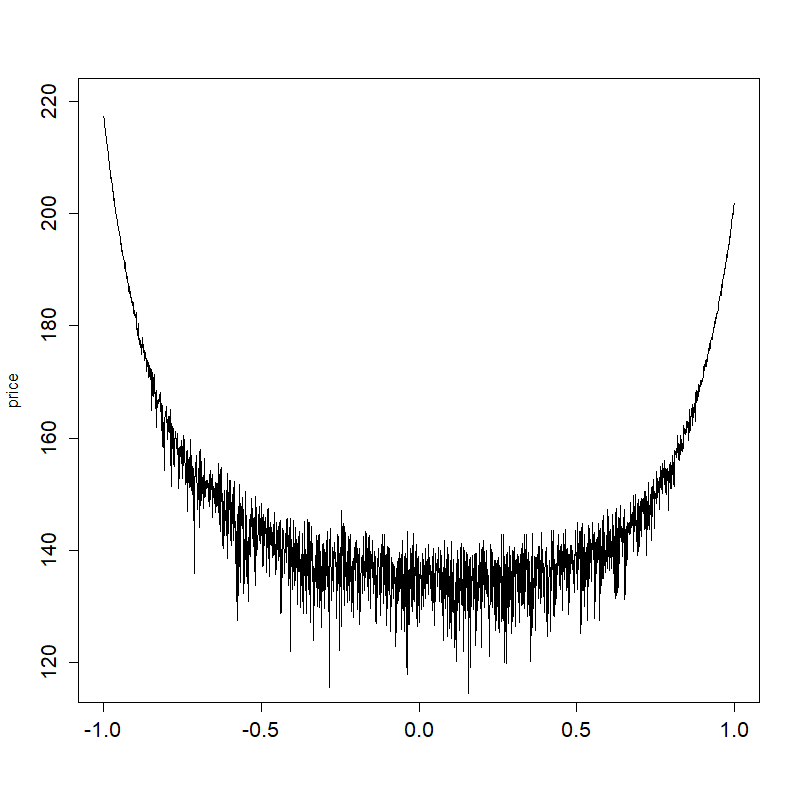
We consider a continuous-time financial model with time horizon . An economic agent will receive, at time units of a derivative written on some non-traded stock and seek to evaluate the price she is willing to pay for that. This is the classical problem of pricing in mathematical finance, but as the investor is facing trading restriction, she wants to estimate the risk premium related to this lack of marketability. Indeed, in a complete market when can be dynamically traded, the derivative price is given by its discounted expected value under some martingale measure and the marketability risk premium is null. As this approach is not feasible when is not dynamically traded, we assume that the investor hedges her position on the derivative on by trading another “similar” liquid asset The asset must be thought of as a related index or as another stock from a closed industry sector. We follow [18] and use the reservation price concept in order to value the illiquidity of . The reservation price is the price which leaves the agent indifferent between paying at time and receiving units of shares of the derivative on at time or doing nothing. This is a preference-based bid price. In the case of a Black-Scholes-like market, when the preferences of the agent are represented by some exponential utility function with risk aversion coefficient , this problem has been well-studied in the literature: see [2, 5, 4, 7] and [17] and the references therein. It is possible to obtain a semi-closed formula for the reservation price which involves the logarithm of the Laplace transform of some function of a lognormal random variable. The expectation in the Laplace transform may be computed with the Monte Carlo method. Nevertheless, we observe that the Monte Carlo method leads to unreliable estimators suffering from very high variance (see Figures 3 and 8). Thus, our first motivation is to find an improved numerical method for the computation of the reservation price.
An alternative method to Monte Carlo is to produce a polynomial approximation. This has been done for an expansion in terms of small in [4, 5], in terms of the correlation between and in [2] and in terms of an aggregate of , and in [12] and [13]. Thus, we first derive polynomial approximations in and show (see Figure 2) that these polynomial approximations can be extremely bad. We take the opportunity to precise the error order of the expansions proposed by Monoyios, as its coefficients are defined using the minimal martingale measure and thus depend on the correlation.
Based on these observations, we propose a new and improved numerical method. For this method, we adapt an idea from [1] and [18], where a modified Laplace method is introduced in order to get a closed form approximation of the Laplace transform of a lognormal random variable. The Laplace method provides asymptotic for the integral of a function indexed on some parameter and exhibiting a sharp peak whose integral is almost equal to the whole integral for large value of the parameter (see [17] for more details about the Laplace method). The resulting asymptotic taken as an approximation can be very accurate not only in the asymptotic setting. The Lambert function, which is the inverse of appears in those approximations. This function has been widely used and study in the last 30 years due to the advent of fast computational methods, see [19]. Here, we adapt the idea of [1] considering a non smooth function of a lognormal random variable. This modified Laplace method allows splitting the reservation price into a deterministic part and a random part, the first one being preponderant in meaningful financial situations, while the second, which is close to one, will help to provide a low variance estimator for the price. For example, this variance may decrease from 5.66 to 0.017. This method also provides some multiplicative decomposition for the value function. We call this method the Lambert Monte Carlo (LMC) method. We show numerically that the LMC method is indeed an improvement of the Direct Monte Carlo (DMC) method in various market situations (see Figures 3 and 8). We also compare the speed of both methods and find numerically that they are of same order. But the number of simulations required for the DMC method to obtain a satisfactory confidence interval can be very large. This is not the case for the LMC method (see Table 3). We refer to [1] for numerical comparison of the LMC method with methods other than polynomial approximation available in the literature as well as a survey on the numerical methods developed to approximate the Laplace transform. Here, we will focus on comparison with series expansion as this is the standard for the computation of the reservation price in the financial literature.
We then apply the preceding results to the case of an agent willing to cover a long position on the non-traded stock. This is a very important issue in management sciences which is often referred to as the restricted stock problem or marketability problem: see [11, 9, 3], or for the real option problem, see [5] and the references therein. The second main result of this paper is to provide a lower and an upper deterministic approximation of the reservation price, the value function as well as an approximation of the optimal strategy and of some Greeks. They are based on our decomposition. We study the efficiency of our approximations in terms of , and and show that they are indeed reliable in various financial situations (see for example Figure 3). They thus provide proxy which need almost no computation time. We also compute the minimum of our lower approximation of the reservation price. Note that the semi-closed expression of the reservation price does not allow such theoretical result to be obtained. We show numerically that is in fact a good approximation of the minimum of . This minimum offers a new perspective for utility-based pricing and hedging. Indeed, may be the optimal choice for an agent selecting between different hedging assets who is willing to choose the one that minimizes the reservation price while retaining the same level of rentability and for which almost no money is invested in the (optimal) hedging strategy. We then show that choosing an hedging asset of correlation and using the (optimal) hedging strategy does not cripple the superhedging probability. We also apply our result to the case of a short position on a put option and provide numerical results.
The paper is organized as follows. In Section 2, we present the financial model. In Section 3, we derive a polynomial approximation in the case of a long stock position. Section 4 provides the decomposition of the reservation price and of the value function using the Lambert function. Then, Section 5 analyses the case of a long stock position, while Section 6 examines the short put case. Section 7 concludes and provides some overview on the applicability of our method to other financial problems. Finally, Section 8 regroups the missing proofs of the paper.
2 The financial model
We consider a continuous time financial model with time horizon and a filtered probability space where the filtration satisfies the usual conditions (right continuous, contains all null sets of ). We denote by (resp. ) the observable price process of some non-traded (resp. dynamically traded) asset. We assume that
where and are correlated standard Brownian motions under the historical probability . The correlation is constant and is denoted by and, as usual, we will write that , where and are independent Brownian motions under . The constants and (resp. and ) respectively represent the expected return (resp. the volatility) of the non-traded and of the traded assets. There is also a riskless bond, with dynamic given by where is the constant riskless interest rate. All discounted values for any process will be denoted by where .
The agent’s initial wealth is denoted by and her trading strategy is denoted by , where is a progressively measurable process that denotes the cash invested in the traded-asset at time . We assume that a.s. for all The agent wealth, starting from an initial wealth and following a self-financed strategy is denoted by and as the agent cannot invest in , her discounted wealth
follows the dynamics:
To value the amount the agent will accept to pay in order to receive the derivative at time , we use a utility-based price. The risk preferences of the agent are modeled by an exponential utility function, which is very popular because of its separability properties. Indeed, in contrast to the power utility function, it gives an explicit representation for the reservation price. Let
where is the constant absolute risk aversion parameter of the agent.
Let be the value function at time for an agent that maximizes her expected utility of terminal wealth at time if in addition she receives units of the European derivative , where is a measurable function whose assumptions will be specified below :
| (1) |
It is possible to find a semi-closed formula for the optimal trading strategy and for the value function using either the dual approach based on martingale techniques (see [14] or [10] and the references therein) or the primal approach. The primal approach (see [4] or [5]) leads to a non-linear Hamilton-Jacobi-Bellman equation that can be linearized using the Hopf-Cole transformation. Please refer to [15], where this transformation is called the distortion method. With a slight adjustment to Section 5 of [4], we determine that :
| (2) |
where is a standard Gaussian law. Note that the parameters of appear only through the Sharpe ratio of . If is bounded from below on , the bid reservation price of units of the derivative is the amount, which leaves the agent indifferent between paying at time and receiving units of at time or doing nothing, i.e., is a solution of the following equation:
| (3) |
If is bounded from above on , the ask reservation price of units of the derivative is the amount, which leaves the agent indifferent between receiving at time and delivering units of at time or doing nothing :
| (4) |
Thus, if is bounded on , we easily determine that :
| (5) |
| (6) | |||||
| (7) |
Thus, we will first search for approximations for and then deduce the results on using (7).
Let and be a measurable function, which is bounded from below on In the following, we will focus on the computation of the bid reservation price of a derivative of the form This includes the bid price of the non-traded stock choosing and where for all We will also get the ask price of a put option (where ) for some , choosing Indeed, .
We will denote by and (resp. and ) the value function of units of (resp. ) and the associated bid reservation price. Similarly, and will be respectively the value function of units of and the ask reservation price of the put.
In the sequel, we will consider several market conditions. Situation 1 of Table 1 presents a meaningful market situation that will be taken as a reference throughout the article. We also introduce two other market situations to observe the effect of a low initial price for the non-traded asset (see situation 2 of Table 1) and a long time horizon (see situation 3 of Table 1).
| T | ||||||||
|---|---|---|---|---|---|---|---|---|
| Situation 1 | 0.1% | 2 | 0.25 | 100 | 20% | 30% | 10% | 20% |
| Situation 2 | 0.1% | 20 | 0.3 | 1 | 35% | 40% | 10% | 20% |
| Situation 3 | 0.1% | 10 | 10 | 100 | 30% | 30% | 5% | 10% |
3 Polynomial approximation
In this section, we search for some polynomial approximation for the reservation price that will be relevant in general market situations. Such an approach was already studied by many authors.
Davis [2] achieved an expansion with respect to using ideas from Malliavin calculus, while Henderson [4] focused on an expansion on and found a similar expression. Later, Monoyios [12, 13] gave a higher order expansion on a parameter involving correlation, risk aversion and the number of claims for the ask reservation price.
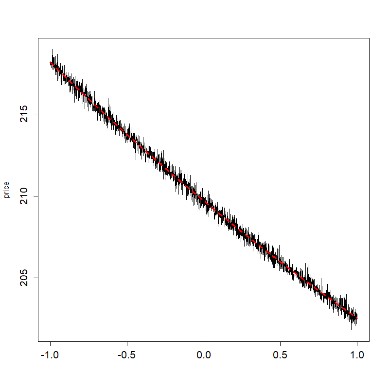
It is worth noting that the Monoyios’s expansions are not Taylor expansions in the sense that some dependence upon remains present in the coefficients, which are defined using the minimal martingale measure. As a consequence, we strongly believe that the error order provided by Monoyios (see Theorem 3 in [13]) may have been misestimated. Nevertheless, his approximation has proven to be reliable for the computation of the ask reservation price of a put option for a very small risk aversion (see Table 1 in [13]). We show in Figure 1 that this approximation remains correct for the computation of the bid reservation price of a stock for very small values of the risk aversion or very high correlation, but that this is no more the case elsewhere.
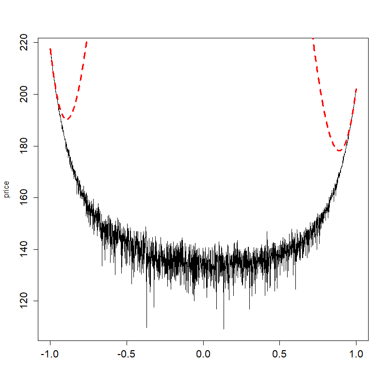
To complete the works of Davis and Monoyios, we propose below a Taylor expansion, when the correlation is close to one, of the bid reservation price of a non-traded stock. We will in particular show that Taylor expansions remain an extremely bad approximation, when the correlation is not very close to one (see Figure 2).
Let and be the cumulant-generating function of i.e., . Since is a log-normal random variable, exists only for negative values of . Furthermore, as has moments of any orders, the function is on with limits at for all derivatives. So, the function admits a Taylor expansion up to an arbitrary order at and have the following decomposition :
| (8) |
The coefficients are called the cumulants of the distribution of . As a function of , the reservation price can be written as follows (see, (6) with ):
| (9) |
with and where the coefficients can be expressed in terms of the sequence for any arbitrary order . We have computed the coefficients in (9) up to order 4, see Section 8.1 in the Appendix for more details on the computation. As a first step, we get the following expression :
Using the notation and , we then get that :
Note that corresponds to the expectation of computed under the unique probability measure which turns the discounted value of the traded asset into a martingale in the complete case, i.e., when . Indeed,
We now perform some numerical computations for the market situation 1 (see Table 1).
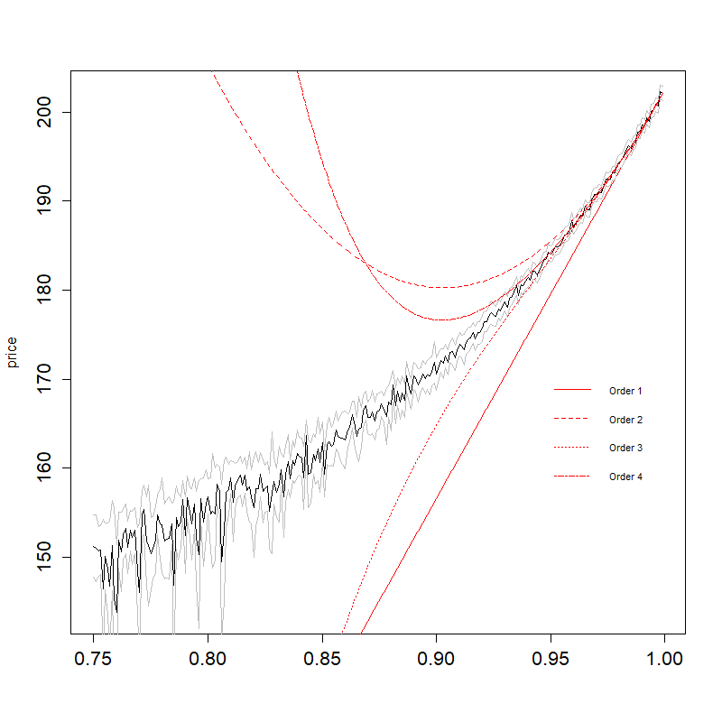
Looking at Figure 2, Taylor expansions of all orders are unreliable approximations when the correlation is lower than , and higher orders of expansion lead to greater errors. Thus, Taylor expansions (and general polynomial expansions) do not give approximations of the bid reservation price that remains reliable on at least for reasonable market situations. They also do not provide an estimation of the error between the price and the expansion.
4 Lambert approach
The polynomial method has been shown to be irrelevant for our purpose. Thus, we now provide another approach in the spirit of [1], where we split the reservation price into a deterministic part and a random one. The bid reservation price can be written as the logarithm of the Laplace transform of some function of a lognormal random variable and of an indicator function. Following [1] and [18], we apply a modified version of the Laplace method (see [17, Chapter 4]) to compute the integral in the Laplace transform. In his thesis [18], Rojas-Nandayapa derived an approximation of the Laplace transform of a lognormal random variable using a saddle point approximation. Later, Asmussen and all derived rigorously in [1] the same approximation using a modified Laplace method. We generalize their approach to . We approximate by a polynomial function and we get the maximum of out of the integral, see (11) and (12). This leads to a multiplicative decomposition of the Laplace transform and thus, an additive decomposition for the bid reservation price. Based on this decomposition, we will propose in the next sections a deterministic lower and upper bound for the reservation price and the value function. We will see that those bounds are indeed accurate. We will provide interesting results on the lower bound as a function of and . We will also propose an improved numerical method for the computation of the reservation price, based on an estimator with a lower variance, by performing the Monte Carlo method only on the random part, see Figures 3 and 8.
We start with the decomposition of the Laplace transform of the random variable where and is a measurable function that is bounded from below on . Note that [1] studies the case where and . As is bounded from below on , is well defined for all :
Let and be a measurable function, that is bounded from below on . Set , and for all . There is a simple relation between and . Indeed, using (6) with , we obtain that
| (10) |
We now propose a decomposition of . To do that, we employ a kind of Taylor expansion of . At this stage, we do not specify with as we use different values for and whether or not. For all ,
| (11) | |||||
where for all , we have set and
| (12) |
Note that . Moreover, is continuous if and only if .
We seek to remove the integral in (11) of the maximum of . Thus, we aim to minimize : to do that, we first study . Obviously, is , and for all , As , for all , we have . Assume now that . Then, if and only if At this point, we need the inverse function of .
Definition 4.1.
The Lambert function is the inverse function of
We provide some properties of in the Lemma 8.1 in the Appendix : in particular, on . The computation of the minimum of is performed in Lemma 8.3 in the Appendix. This provides the following multiplicative decomposition of , which extends [1, Proposition 2.1].
Theorem 4.2.
Let , and be a measurable function that is bounded from below on . Let be any real number if and if . Moreover, suppose that
| (13) |
Then, where with the convention that :
With Theorem 4.2, we can derive a decomposition of the reservation price and of the value function for a derivative with payoff .
Theorem 4.4.
Let and be a measurable function that is bounded from below on . Let and if or be any real number if . Moreover, suppose that
| (14) |
Then,
| (15) | |||||
| (16) | |||||
| (17) |
where is defined in Theorem 4.2 with and for all
We call the deterministic part of and its random part. Moreover,
| (18) | |||||
| (19) | |||||
| (20) |
Proof 4.5 (Proof of Theorem 4.4).
Remark 4.6.
With the decomposition provided by (15) and (18), we perform a Monte Carlo method only on the random part of the reservation price or of the value function (see (17) and (20)). So, we need to choose and such that is as small as possible, i.e., such that is close to This is possible since differences between functions and their Taylor expansion of order one in zero appear. We call this the Lambert Monte Carlo (LMC) method. We show below that it is indeed numerically efficient: see Figures 3 and 8.
5 Long stock position
In this part, we focus on the case of a long stock position on the non-traded stock, which is, as already mentioned, of great importance in management science. After giving the decomposition of the reservation price, we study the quality of the deterministic part as an approximation of the reservation price. We also give an approximation of the optimal strategy and of the Greeks. We provide numerical illustrations of all these quantities. We also examine the problem of selecting the right hedging asset . We show that choosing an asset with the correlation (the minimum of the deterministic part as a function of ) with provides a minimum reservation price, as well as a minimum cash position invested in .
5.1 Decomposition of the reservation price and of the value function
The next theorem is a direct consequence of Theorem 4.4. Recall that is the bid reservation price of units of and is the associated value function.
Theorem 5.1.
Let Then, , where
| (21) | |||||
| (22) |
Moreover, where
| (23) | |||||
Remark 5.2.
As and , we get that and the deterministic part (resp. ) is a lower bound for (resp. ).
5.2 Deterministic approximations of
We have seen that provides a deterministic lower bound for the reservation price (see Remark 5.2). Using the Lambert function, we also provide a deterministic upper bound for called and study the quality of both bounds. Let
| (24) | |||||
Theorem 5.4.
We have that and that Moreover,
| (25) | |||||
| (26) |
where .
The bounds in (25) easily apply to and show that is small relative to :
Having bounds that only depend on and legitimizes the use of and as uniform approximations of the reservation price in terms of
or . For example, if , then , and if , .
When and goes to infinity, goes to infinity (see Lemma 8.1 in the appendix) and (25) implies that goes to .
We will see that numerically, provides a better approximation when and are large enough : see Figure 5.
In contrast, when and goes to or goes to , goes to 0 (see Lemma 8.1 in the appendix) and (26) implies that goes to . So,
is sharp for small values of and or high values of : see Figure 5.
The limits in terms of and are less straightforward.
Let be such that and Let be such that .
Proposition 5.6.
The functions , and are , positive and bounded. Moreover,
| (27) | |||||
| (28) | |||||
| (29) |
Recall that is an approximation at order of near (see (9)).
Thus, unlike , the upper bound is not biased for high positive correlation. Note that (27) shows that
Thus, small values of and reduce the bias between and for high positive correlations.
When the risk aversion goes to , goes to zero, which is the subhedging price of When the risk aversion goes to goes to , where is the expectation of under the minimal martingale measure, i.e. the minimal variance price of the claim , see [20] and [21]. Recall that the minimal variance price is the initial wealth that minimizes the quadratic hedging error under
the historical probability.
We compute now some Greeks like quantities for the lower bound . We are particularly interested in the Cega i.e. the sensitivity of the long stock position to a change in the correlation. We also compute the sensitivity with respect to .
Proposition 5.8.
We have that
Note that the dynamic version of the (true) sensitivity of the long stock position to a change in the correlation is present in the expression of the optimal strategy, see (30).
5.3 Numerical applications for the reservation price
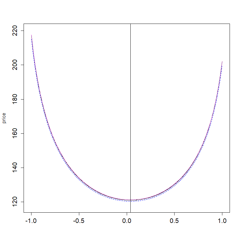
We now provide numerical simulations to illustrate the performance of the Lambert Monte Carlo (LMC) method in comparison with the Direct Monte Carlo (DMC) method and also the quality of our deterministic approximations and of the reservation price . We also plot the correlation that minimizes , which will be studied in Section 5.5 below.
| LMC method | DMC method | Lower bound | Upper bound | |
|---|---|---|---|---|
We see in Figure 3 that the LMC estimator of the bid reservation price of does not suffer from high variance, as is the case for the DMC estimator. For example, in situation 1 of Table 1 with and , the variance of the DMC (for simulations per point) is 5.66 and that of the LMC method is 0.017. We see that and are indeed good approximations of . Moreover, the quality of the estimates given with the LMC method is much less sensitive to parameter variation than the one given by the DMC method (for a fixed number of simulations) as showed in Table 2. Indeed, for large values of the DMC method provides wrong estimates, while the estimations performed with the LMC method remain correct.
This can be explained by the fact that the DMC estimator needs more than simulations to be pertinent for higher value of .
On the other hand, the quality of the LMC estimator is relatively stable for all values of for simulations and this estimator is very close to the real price. Note that this abnormality can also be observed when working with high risk aversion or with high initial price .
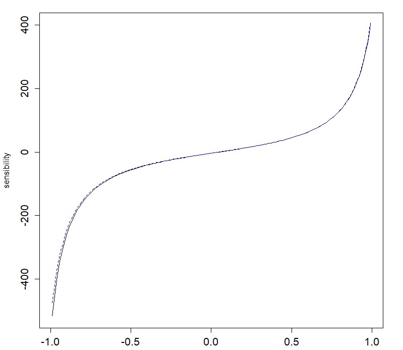
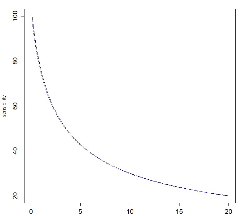
We now discuss the sensitivity of the price with respect to and . We show numerically that the sensitivity of can be very close to the one of (with respect to and ), see Figure 4. The two curves are indeed very close even when is not necessarily a good approximation of . For example, when , the relative error between and is equal to and when , the relative error between and is equal to .
We now propose other simulations in the situations 2 and 3 of Table 1 in order to illustrate the quality of and .
We see in Figure 5 that the upper deterministic approximation performs better when and are small (situation 2), while when and are large (situation 3), the lower bound is clearly more accurate. For the numerical values of situation 3 of Table 1, the DMC does not work because of rounding issues. Moreover, note that the minimizer of the reservation price in is indeed close to the minimum of the deterministic part , even in situation 3, where has no reason to be a good approximation for .
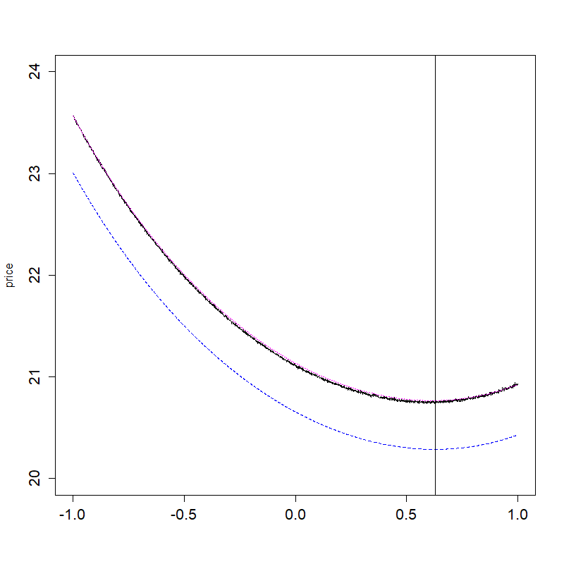
Market Situation 2,
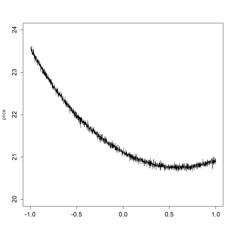
Market Situation 2,
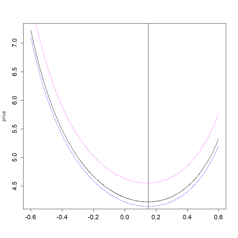
Market Situation 3,
We now comment on the computational time of both the LMC and the DMC methods. In the market situation 1 of Table 1 with and , the execution time111CPU specification : Intel Core i5 - 7300U 2.60GHz, RAM specification : 8GB DDR3 of the LMC (resp. DMC) method for the computation of the reservation price and the Confidence Interval (CI) with simulations is 2.72 (resp. 2.10) milliseconds. For simulations, it is 229.14 (resp. 214.91) milliseconds. So, both methods take roughly the same time to produce a given price and CI. Indeed, most of the execution time of the LMC and the DMC methods comes from the simulation of random variables and the part dedicated to the computation of the Lambert function is negligible.
In contrast to the LMC method, the number of simulations required for the DMC method to obtain a satisfactory CI can be very large. This phenomenon is illustrated in Table 3. We see that for some values of the correlation, the DMC method needs simulations to deliver an appropriate CI while simulations are enough for the LMC method. Note that in the situation 1 of Table 1 and with our computer, the DMC method fails to deliver a CI of length smaller than for as it needs more that simulations.
| LMC method | DMC method | Bounds | ||||
|---|---|---|---|---|---|---|
| Time | Time | Lower bound | Upper bound | |||
| 179.97 | 181.72 | |||||
| 160.67 | 162.11 | |||||
| 139.42 | 140.57 | |||||
| 0.15 | 18020.96 | 128.39 | 129.40 | |||
| 0.15 | 170.80 | 122.62 | 123.57 | |||
| 0.16 | 172.85 | 120.44 | 121.37 | |||
| 0.16 | 16974.27 | 121.37 | 122.32 | |||
| 0.17 | 170.00 | 125.73 | 126.73 | |||
| 0.15 | 18476.06 | 134.93 | 136.06 | |||
| 0.19 | 172.26 | 153.23 | 154.62 | |||
| 0.15 | 17.38 | 169.91 | 171.57 | |||
We now compute the deterministic bounds for and of Theorem 5.4 in order to quantify the precision of our deterministic approximations of and to determine how sharp they are. We start with the lower bounds of . In the market situation 1 of Table 1, we have that . The other bound in (25) is sharper (for and , it is between 0.9910 and 0.9956). Thus, the reservation price is well-explained by . So in this situation, the two bounds for are indeed very close. This is not the case in the situation 3 of Table 1. Indeed, we have while the other bound in (25) is much tighter, as seen in Table 4.
| 0.8735 | 0.8735 | 0.8688 | 0.8567 | 0.8301 | |
| 0.9936 | 0.9944 | 0.9946 | 0.9944 | 0.9935 | |
| 0.9949 | 0.9956 | 0.9956 | 0.9955 | 0.9948 |
We now compute the upper bounds of in (26). In the market situation 1 of Table 1, we have that . The other bound is between 1.0035 and 1.0106 for and The bounds are again very close, and the reservation price is also well explained by . In the market situation 3 of Table 1, we find that and the values of the other upper bound in (26) are greater than even though is still a correct approximation of (see Figure 5).
As a conclusion to this section, we have seen that and are reliable approximations of the reservation price and are obtained without any computation time.
5.4 Optimal strategy and value function
We focus now on the optimal strategy for (1), i.e., the strategy that maximizes the expected utility in (1), when . As we consider a bid reservation price instead of an ask reservation price (see (5)), we need to slightly adapt the arguments of Monoyios (see (29) in [13]). For all and , we obtain that
| (30) |
where is the dynamic version of , i.e., where is the value function at if and For all and , as for (6), we determine that
| (31) |
The computation of the optimal strategy involves the partial derivative of Therefore, numerical issues may appear because the DMC method performs badly even for : see Figure 3. Monoyios (see Corollary 1 in [12] or Section 4.1.1 in [13]) addresses this issue by computing the series expansion of the partial derivative in (30). However, we have seen in Section 3 that the series expansion can be extremely imprecise for especially when is not very small and is not near 1. Thus, we propose to use in (30) a dynamic version of our decomposition of the reservation price:
where for all and , and
| (32) | ||||
Using (47) in the Appendix, we determine that
| (33) |
Thus, we propose to approximate with the deterministic strategy defined for all and by
| (34) |
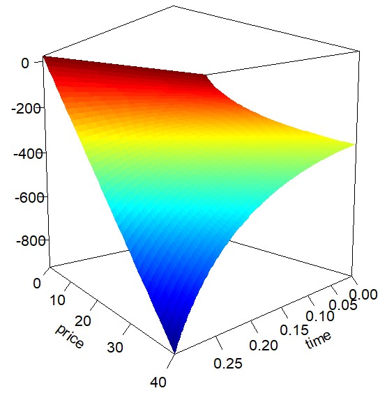
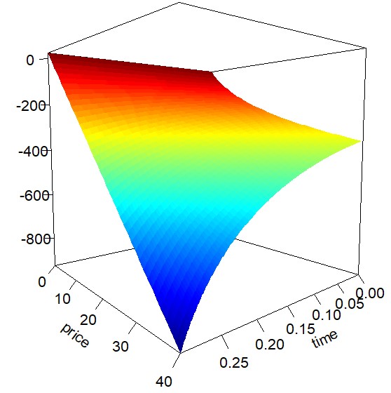
This strategy avoids taking the partial derivative and the related numerical issues. We do not provide any theoretical results regarding the quality of this approximation, but we show numerically in Figure 6 that both strategies are indeed close. Note that in the market situation 1 of Table 1, when and , the value function is very small as So, providing numerical approximations for is not meaningful. We thus turn to the market situation 2 of Table 1 with and
It is also interesting to compare with the value function defined in (1).
| Sd |
|---|
We see that the deterministic approximations of are reliable. Moreover, looking at Table 5, is much more precise than . Indeed, in Figure 5, is a better approximation of than . However, , the expected utility computed with the strategy (34), provides an even better approximation. We have seen numerically that this is true in other market situations, which confirms the relevance of the approximated optimal strategy.
5.5 Selecting a hedging asset
One may examine the problem of pricing and hedging from a different point of view. Assume that an agent has the choice between different hedging assets and chooses the one that minimizes the reservation price with the same level of rentability: i.e., , and are fixed (and thus also the rentability), and she minimizes in . Indeed, as is a bid price, the agent may want to pay as little as possible222 Note that the value function and the reservation price share the same minimizer in see (7). Thus, it is clear that the market embedded with the correlation that minimizes the bid reservation price is always the worst choice for an agent who wants to maximize her expected utility.. Unfortunately, the variation and the minimum of the reservation price (as a function of ) are very difficult to study. However, this can be done for the deterministic part , as stated in the next proposition, and the numerical applications of Section 5.3 suggest that the minimum of , is in fact a good approximation of the real minimum of the reservation price. It is worth noting that even if and appear to be similar (see (59) and (61) in the Appendix), the study of the variations of is much more difficult. In particular, we were unable to find the minimum of .
Proposition 5.10.
Let
| (35) |
If , is increasing on . If ,
is decreasing on .
Now, assume that . Then,
is decreasing on and increasing elsewhere and
Moreover,
| (39) | |||||
| (40) |
The correlation has another interpretation related to the deterministic strategy , where denotes the deterministic strategy introduced in (34) for the correlation for all , as we see in the following proposition.
Proposition 5.12.
Assume . Then,
We know from Section 5.4 that the deterministic strategy is a good approximation of the optimal strategy. Thus, given an agent who buys units of at time and is faced with the choice of an hedging asset, Proposition 5.12 shows that can be interpreted as the correlation between and for which an investor would have no share in the hedging asset at time . This is relevant because the money borrowed for the hedging strategy can be very high, see Figure 6. We now provide similar results for , which denotes the optimal strategy (30) for the correlation . We first give a theoretical answer when is close to and then shows numerically that choosing the correlation can provide the desired effect even when is not small.
Proposition 5.14.
Let , we have that Thus,
| (41) |
Assuming that the agent holds the claims for a very short period of time, Proposition 5.14 shows that an agent who chooses a hedging asset whose correlation is close to should not invest too much money in the hedging asset (see Figure 7). We now show numerically that choosing an hedging asset such that the correlation between and is equal to (or its limit in ) is indeed a good choice for an agent who wants to invest as little as possible on the hedging strategy, even when is not very small.
We then show numerically that even if the agent chooses to hedge herself with the asset with correlation , it does not cripple the superhedging probability for defined in (34). To do that, we compute a Monte Carlo estimation (with simulations per point and a time step of in the Euler scheme, i.e., 200 rebalances of the strategy) of this probability in the situations 1 and 2 of Table 1 for different values of .
| Situation 1 | Probability | ||||||
|---|---|---|---|---|---|---|---|
| with | CI | ||||||
| Situation 2 | Probability | ||||||
| with | CI |
This suggest that the superhedging probability does not change much when varying the correlation and justifies the choice of a hedging asset with correlation .
We finish with an approximation of for small and large values of .
Lemma 5.16.
We determine that
| (42) |
where . Assume that Then, .
The following table shows the efficiency of the first-order approximation in (42).
6 Short put position
We now study the case of a short position on a put option with payoff , where . Recall that and are respectively the value function of a short position on units of a put option and its ask reservation price, i.e., and : see (5).
Theorem 6.1.
Let and suppose that
| (43) |
Then, where
Moreover, where
Proof 6.2 (Proof of Theorem 6.1).
We now provide numerical simulations for the reservation price .
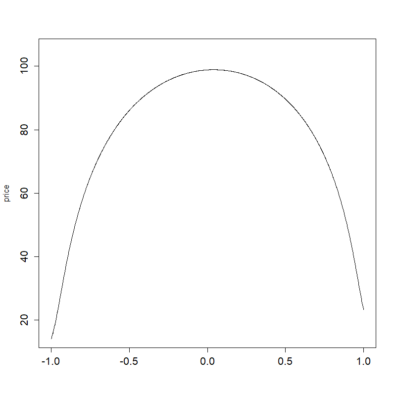
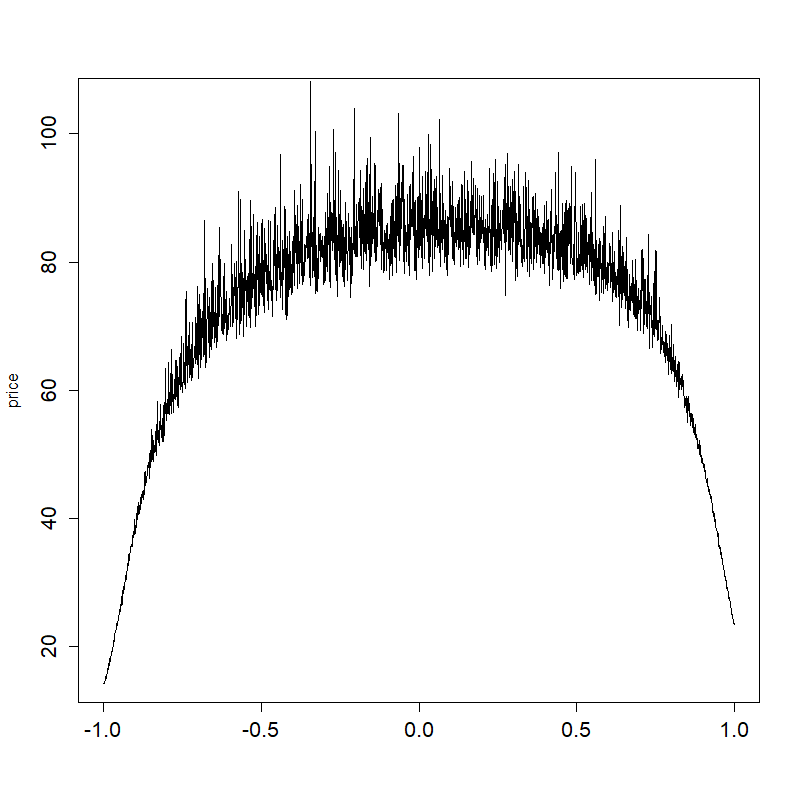
As in the long stock position case, the DMC estimator provides an estimator with high variance. Conversely, the LMC estimator exhibits low variance. For example, in the market situation 1 of Table 1, with and , the variance is 4.745 for the DMC method (for simulations per point) while the variance of the LMC method is 0.007. The results are similar in the market situation 2 of Table 1 with and with simulations per point.
We now propose numerical simulations for the value function. In the market situation 1 of Table 1, when , and , and are large enough to be relevant for correlation such that . Indeed, for higher values of , the values of and are very small and the numerical estimations are not relevant (for example, if , and ).
| CI | |||||
|---|---|---|---|---|---|
7 Conclusion and discussion
We have presented a methodology to obtain an improved Monte Carlo estimate of the reservation price of a derivative in a Black-Scholes market.
The reservation price is a utility based price and is useful in an incomplete market where the underlying asset cannot be traded dynamically, hence the pricing by the martingale approach is not feasible. An alternative asset which can be traded dynamically in the same market is then used to hedge the position of the investor. The (bid) reservation price is the amount which leaves the trader indifferent to have the derivative or not. The reservation price can be written as the logarithm of the Laplace transform of a function of a log-normal random variable, that we have decomposed in two parts using the Lambert function. The first one is deterministic and the second one can be seen as an expected value which is closed to one.
This decomposition provides an improved numerical method called the "LMC method". In the case of a long position on the non-traded asset, it allows the construction of upper and lower deterministic bounds for the reservation price and the value function, as well as an approximation of the optimal strategy and of some Greeks. The lower bound is a reliable approximation of the (bid) reservation price, which can be studied analytically and we obtained information about its behavior as well as its minimum . We have showed that this minimum may be the optimal choice for an agent who want to select an hedging asset that minimizes the reservation price and also the cash invested in retaining the same level of rentability. We have also shown numerically that choosing such a does not cripple the superhedging probability.
We were also able to control the error between the bounds and the reservation price.
One may ask if the same conclusions apply to the case of a long position on a call option.
The decomposition of the bid reservation price of a long position on a call option can be obtained using similar methods (the details are not provided in the paper for sake of brevity).
We introduce an adapted notion of in- and out-of-the-money call options. An in-the-money (resp. out-of- or at-) call option of strike is an option, where (resp. or ), where
see Theorem 5.1 for the definition of . We easily see that
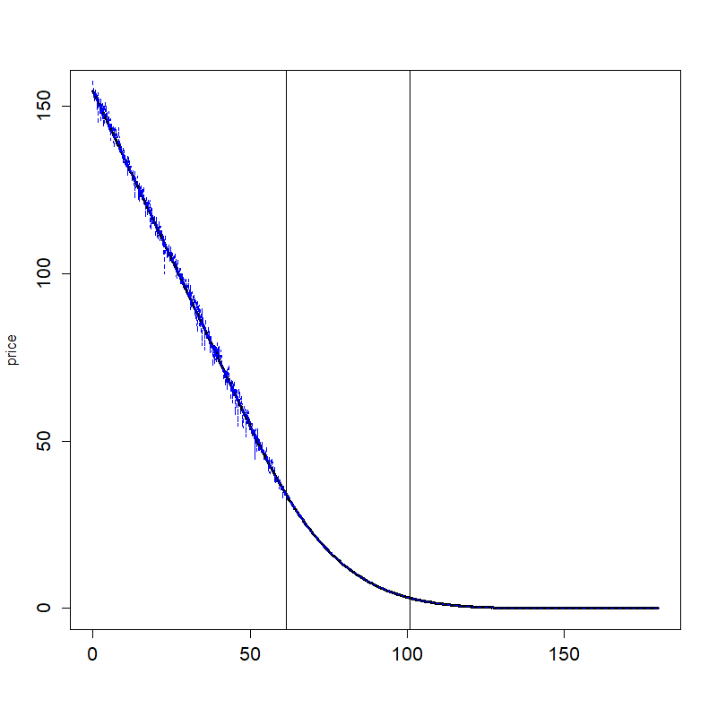
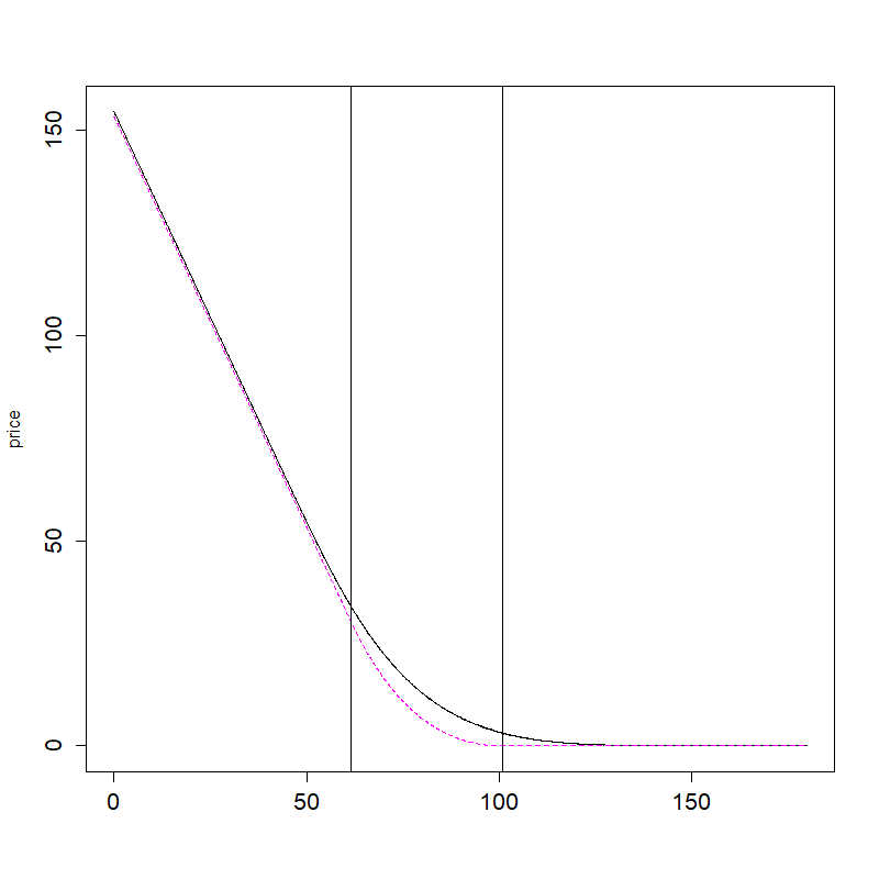
The LMC method provides better results for in- and out-of-the-money call options, but for at-the-money call options, it is not clearly better than when using the DMC method. Moreover, if or the deterministic part of the decomposition of the reservation price is a good approximation of the price. This is illustrated in Figure 9 below.
One may ask to what extend one can go beyond the Black-Scholes model. One possible generalization would be to have several tradable assets to cover . To the best of our knowledge, no semi-closed formula like (6) has been derived in this case. Another generalization could be to consider that the parameters of and are time dependent. In this case, it is still possible to obtain a formula like (6) and to perform our method. Now if the coefficients are also stochastic, Tehranchi showed in [22, Remark 5] that the reservation price can always be written in a semi-closed formula though the resulting expression can be very different from (6) and does not necesseraly imply the Laplace transform of a function of a lognormal random variable. One last possible generalization would be to consider a random drift coefficient (at time ) with a gaussian prior. This is useful in the context of drift erroneous estimate. In that situation, Monoyios provides in [12] a semi-closed expression for the reservation price depending on the minimal martingale measure but still very similar to (6). Moreover, one can easily show that the value of the non traded asset at time still follow a lognormal distribution under the minimal martingale measure. This means that our method would also be appropriate in this case.
8 Appendix
8.1 Proof of Section 3
Recall that where has standard normal distribution and that . Let and Then, . We also introduce The reservation price takes the following form (see, (6) with )
| (44) |
We first compute the Taylor expansion of order at of . For that we use (8) for and as we obtain that
| (45) |
with will denote in the sequel a function such that . Now, we compute the Taylor expansion of order of the powers of .
Plugging the previous expressions in (45), we find that where,
We now proceed to the expansion of in (44).
Recalling that and noting that for all , , we determine that
The expression of the coefficients , , , and in Section 3 follows.
8.2 Proofs of Section 4
8.2.1 Properties of the Lambert function
In this section, we provides some useful properties of the Lambert function that will be used in the proofs of our results. By definition, has the following properties:
| (46) |
Lemma 8.1.
The Lambert function is strictly increasing and
| (47) |
Moreover, admits a Taylor expansion around :
Finally, .
Proof 8.2 (Proof of Lemma 8.1).
First, is clearly , being the inverse of . Now, we differentiate (46) and obtain that for ,
| (48) | |||||
where we have used for the last equivalence the fact that and (46).
As , is strictly increasing. Recalling that is , we determine that
Using (46) and (47), and . Now differentiating (48), we determine that for
and . Finally, as , (46) provides that
8.2.2 Proof of Theorem 4.2
Theorem 4.2 provides a multiplicative decomposition of the Laplace transform of a function of a log-normal random variable. For that, we need to find the minimal value of (see (12)). This is the purpose of Lemma 8.3. Fix Let be defined on by
Lemma 8.3.
Let and . Let be any real number if and otherwise. Then, reaches its minimum value in . Moreover,
| (49) | |||||
| (50) |
Proof 8.4 (Proof of Lemma 8.3).
We first study . Then, we use (12) to link the minima of and of according to the values of . As , for , we have . Letting , as is strictly increasing and using (46), we obtain that
which gives the variations of . Moreover, using (46),
As , we determine that reaches its minimum value in and that (50) holds true.
We now study if . As , is continuous.
Assume first that . We show that reaches its minimal value at As (46) implies that
| (51) |
As (51) is equivalent to , (12) and (50) show that
| (52) |
As on , it also shows that is decreasing on and increasing on .
Now, on , we distinguish two cases. First, assume that . Then, and
is increasing on . Thus, reaches its minimum value in
If now , using (51) again, we find that .
Therefore, is
decreasing on and increasing on . Thus, and are two potential minima. However, using (52), we determine that
and we conclude that reaches its minimal value at
Suppose now that . This implies that .
Indeed, using (46) and ,
We want to show that reaches its minimum value at Then, as ,
Assume first that , then .
As on , is decreasing on . Moreover, on and is decreasing on and increasing on
Thus, reaches its minimum value at .
Assuming now that , we determine that . Thus, as on is decreasing on and increasing on Moreover, on , and is decreasing on and increasing on . Thus, and are two potential minima. Using (52), we determine that
and we conclude that reaches its minimum in .
We are now in position to prove Theorem 4.2.
Proof 8.5 (Proof of Theorem 4.2).
We perform the Laplace method on (11) and thus, get out the maximum of of the integral. This gives the deterministic part of the decomposition. Then, an affine change of variable is applied to the remaining integral in order to retrieve the required expression.
Let and . Let be any real number if and otherwise. Assume that (13) holds true.
We set and .
Using (11), we have that
| (53) |
Recall that when , we have chosen . Thus, (13) and Lemma 8.3 imply that Using (49) and (50), we determine that
| (54) |
Then, (53) and (54) with the change of variable and the fact that (see (46)) imply that
| (56) |
Letting , we find that
We remark that . This is trivially true if . If as
which is true by (13). Thus, and
Assume that Then,
Thus, as ,
The same obviously holds true when with the convention . Thus, we get that
Therefore, (56) implies that
8.3 Proofs of Section 5
For ease of notation, we introduce the functions and
| (57) | ||||
| (58) |
Then, , , , and , where
| (59) | ||||
| (60) | ||||
| (61) | ||||
| (62) |
8.3.1 Proofs of Subsection 5.2
Proof 8.6 (Proof of Theorem 5.4).
Assume for a moment that we have proved that for all
| (63) |
Then, as , Remark 5.2, (61) and (63) show that Then, follows from (23) and (7).
We prove now (63). Using the Jensen inequality for the convex function , we obtain that
And so, using Remark 5.2, we determine that Then, as for all , we have that
where Composing with the logarithm function and using the inequality yields
| (64) |
which combined with yields in turn the lower bound for .
Now, we prove (25) and (26).
As we find that
as . Moreover, using (61) and (64), As , using (59), we obtain that
Proof 8.7 (Proof of Proposition 5.6).
The proof relies on the properties of the Lambert function given in Lemma 8.1. As , we find that and . Lemma 8.1 imply that and are and that
| (65) |
As , the first limits in (27) and (28) are proved. The case when goes to is treated similarly. We deduce that and are bounded on .
Recalling (65), we obtain that
Since is continuous on (recall that is continuous), is bounded, and since , is also bounded.
Using Lemma 8.1, we determine that and Thus,
8.3.2 Proofs of Subsection 5.4
Proposition 5.8 gives the expression of and computed from the lower bound at time .
Proof 8.8 (Proof of Proposition 5.8).
8.3.3 Proofs of Subsection 5.5
Proposition 5.10 gives the expression of the minimum of as well as the value of at that minimum. The resulting minimum is then expanded in Lemma 5.16 using the Taylor expansion of the Lambert function given in Lemma 8.1. Proposition 5.12 highlights the link between the deterministic strategy given in (34) and . Proposition 5.14 gives the expression of the correlation between and for which an agent would not invest much in in the case of a short maturity.
Proof 8.9 (Proof of Proposition 5.10).
As and for all , (8.8) shows that the sign of is the sign of . Supposing first that , then for . If now
For the second equivalence, we have composed by the reciprocal function of and for the fourth one by (see (46)).
Suppose now that . Then, for . If now , we prove as before that if and only if . The results for the variation of are as follow.
Setting then Assume now that ,
| (66) | |||||
where we have used (46) for the third equality (as ) and for the fourth one as , and thus . It follows that
Proof 8.11 (Proof of Proposition 5.14).
References
- [1] Asmussen, S. and Jensen, J.L. and Rojas-Nandayapa, L. (2016). On the Laplace Transform of the Lognormal Distribution. Methodol Comput Appl Probab (18), 441-458.
- [2] Davis, M.H.A. (2006). Optimal hedging with basis risk. Kabanov, Y., Liptser, R. and Stoyanov, J., Eds., From Stochastic Calculus to Mathematical Finance, Springer-Verlag, Berlin, 69-187.
- [3] Finnerty, J.D. (2012). An Average-Strike Put Option Model of the Marketability Discount. The journal of Derivatives, 19 (4), 53-69.
- [4] Henderson, V. (2002). Valuation of claims on nontraded assets using utility maximization. Mathematical Finance 12 (4), 351-373.
- [5] Henderson, V. and Hobson, D.G. (2002). Real option with constant relative risk aversion. Journal of Economic Dynamics & Control 27, 329-355.
- [6] Henderson, V. and Hobson, D.G. (2004). Utility indifference pricing-an overview. Volume on Indifference Pricing
- [7] Hobson, D.G. (1994). Option pricing in incomplete markets. Unpublished manuscript
- [8] Hodges, S. and Neuberger, A. (1989). Optimal replication of contingent claims under transactions costs. Review of futures markets (8), 222-239.
- [9] Kahl, M. and Liu, J. and Longstaff, F. (2003). Paper Millionnaires: How Valuable Is Stock to a Stockholder Who Is Restricted from Selling It? Journal of Financial Economics 67, 385-410.
- [10] Karatzas, I. and Shreve, S. (1998). Methods of Mathematical Finance New-York: Springer-Verlag
- [11] Longstaff, F. (1995). How Much Can Marketability Affect Security Values?. The Journal of Finance 50, 1767-1774.
- [12] Monoyios, M. (2007). Optimal hedging and parameter uncertainty. IMA Journal of Management Mathematics 18, 331-351.
- [13] Monoyios, M. (2004). Performance of utility-based strategies for hedging basis risk. Quantitative Finance 4, 245-255.
- [14] Rouge, R. and El Karoui N. (2000). Pricing via utility maximization and entropy. Mathematical Finance 10 (2), 259-276.
- [15] Zariphopoulou, T. (2001) A solution approach to valuation With unhedgeable risks. Finance and Stochastics 5(1), 61-82.
- [16] Henderson, V. and Liang, L. (2014). Pseudo Linear Pricing Rule for Utility Indifference Valuation. Finance and Stochastics 18 (3), 593-615.
- [17] Bruijn, N. G. (1961). Asymptotic Methods in Analysis. Amsterdam: North-Holland Pub. Co.
- [18] Rojas-Nandayapa, L. (2008). Risk probabilities: asymptotics and simulation. PhD Dissertations, Department of Mathematics, Aarhus University.
- [19] Corless, R. M. (1996). On the LambertW function. Advances in Computational Mathematics 5, 329-359.
- [20] Duffie, D., Richardson, H. R. (1991). Mean-Variance Hedging in Continuous Time. The Annals of Applied Probability 1 (1), 1-15.
- [21] Schweizer, M. (1992). Mean-variance hedging for general claims. The Annals of Applied Probability 2 (1), 171–179.
- [22] Tehranchi, M. (2004). Explicit Solutions of Some Utility Maximization Problems in Incomplete Markets. Stochastic Processes and their Applications 114, 109-125.
