Abstract

We present MAPFF1.0, a determination of unpolarised charged-pion fragmentation functions (FFs) from a set of single-inclusive $e^{+}e^{-}$ annihilation and lepton-nucleon semi-inclusive deep-inelastic-scattering (SIDIS) data. FFs are parametrised in terms of a neural network (NN) and fitted to data exploiting the knowledge of the analytic derivative of the NN itself w.r.t. its free parameters. Uncertainties on the FFs are determined by means of the Monte Carlo sampling method properly accounting for all sources of experimental uncertainties, including that of parton distribution functions. Theoretical predictions for the relevant observables, as well as evolution effects, are computed to next-to-leading order (NLO) accuracy in perturbative QCD. We exploit the flavour sensitivity of the SIDIS measurements delivered by the HERMES and COMPASS experiments to determine a minimally-biased set of seven independent FF combinations. Moreover, we discuss the quality of the fit to the SIDIS data with low virtuality $Q^{2}$ showing that, as expected, low-$Q^{2}$ SIDIS measurements are generally harder to describe within a NLO-accurate perturbative framework.

1 Introduction

Unpolarised collinear fragmentation functions (FFs) [1] encode the non-perturbative mechanism, called hadronisation, that leads a fast on-shell parton (a quark or a gluon) to inclusively turn into a fast hadron moving along the same direction. In the framework of quantum chromodynamics (QCD), FFs are a fundamental ingredient to compute the cross section for any process that involves the measurement of a hadron in the final state. Among these processes are single-hadron production in electron-positron annihilation (SIA), semi-inclusive deep-inelastic scattering (SIDIS), and proton-proton collisions.

An analysis of the measurements for one or more of these processes allows for a phenomenological determination of FFs. Measurements are compared to the predictions obtained with a suitable parametrisation of the FFs, which is then optimised to achieve the best global description possible. The determination of the FFs has witnessed a remarkable progress in the last years, in particular of the FFs of the pion, which is the most copiously produced hadron. Three aspects have been investigated separately: the variety of measurements analysed, the accuracy of the theoretical settings used to compute the predictions, and the sophistication of the methodology used to optimise FFs. In the first respect, global determinations of FFs including recent measurements for all of the three processes mentioned above have become available [2]; in the second respect, determinations of FFs accurate to next-to-next-to-leading order (NNLO) [3, 4] or including all-order resummation [5] have been presented, albeit based on SIA data only; in the third respect, determinations of FFs using modern optimisation techniques that minimise parametrisation bias [4], or attempting a simultaneous determination of the parton distribution functions (PDFs) [6], have been performed. These three aspects have also been investigated for the FFs of the kaon [7, 8, 4, 9, 10, 6].

This paper presents a determination of the FFs of charged pions, called MAPFF1.0, in which the most updated SIA and SIDIS measurements are analysed to next-to-leading order (NLO) accuracy in perturbative QCD. Our focus is on a proper statistical treatment of experimental uncertainties and of their correlations in the representation of FF uncertainties, and on the efficient minimisation of model bias in the optimisation of the FF parametrisation. These goals are achieved by means of a fitting methodology that is inspired by the framework developed by the NNPDF Collaboration for the determination of the proton PDFs [11, 12, 13, 14, 15, 16], nuclear PDFs [17, 18], and FFs [4, 19]. The framework combines the Monte Carlo sampling method to map the probability density distribution from the space of data to the space of FFs and neural networks to parametrise the FFs with minimal bias. In comparison to previous work [4, 19], in this paper the input data set is extended to SIDIS and the neural network is optimised by means of a gradient descent algorithm that makes use of the knowledge of the analytic derivatives of the neural network itself [20].

The structure of the paper is as follows. In Sect. 2 we introduce the data sets used in this analysis, its features, and the criteria applied to select the data points. In Sect. 3 we discuss the setup used to compute the theoretical predictions, focusing on the description of SIDIS multiplicities. In Sect. 4 we illustrate the methodological framework adopted in our analysis, specifically the treatment of the experimental uncertainties and the details of the neural network parametrisation. In Sect. 5 we present the results of our analysis, we assess the interplay between SIA and SIDIS data sets and the stability of FFs upon variation of the kinematic cuts. Finally, in Sect. 6 we provide a summary of our results and outline possible future developments.

2 Experimental data

This analysis is based on a comprehensive set of measurements of pion-production cross sections in electron-positron SIA and in lepton-nucleon SIDIS. In the first case, the data corresponds to the sum of the cross sections for the production of positively and negatively charged pions, differential with respect to either the longitudinal momentum fraction $z$ carried by the fragmenting parton or the momentum of the measured pion $p_{\pi}$; the differential cross section is usually normalised to the total cross section (see Sect. 2.2 in Ref. [4] for details). In the second case, the data corresponds to the hadron multiplicity, that is the SIDIS cross section normalised to the corresponding inclusive DIS cross section (see Sect. 3 for details). Multiplicities are measured separately for the production of positively and negatively charged pions.

In the case of SIA, we consider measurements performed at CERN (ALEPH [21], DELPHI [22] and OPAL [23]), DESY (TASSO [24, 25, 26]), KEK (BELLE [27] and TOPAZ [28]), and SLAC (BABAR [29], TPC [30] and SLD [31]). These experiments cover a range of centre-of-mass energies between $\sqrt{s}\sim 10$ GeV and $\sqrt{s}=M_{Z}$, where $M_{Z}$ is the mass of the $Z$ boson. In the case of SIDIS, we consider measurements performed at CERN by COMPASS [32] and at DESY by HERMES [33]. The COMPASS experiment utilises a muon beam with an energy $E_{\mu}=160$ GeV and a ⁶LiD target. The HERMES experiment utilises electron and positron beams with an energy $E_{e}=27.6$ GeV and hydrogen or deuterium target. Both experiments measure events within a specific fiducial region. The features of SIA and SIDIS data are summarised in Tab. 2.1 of Ref. [4] and in Tab. 1, respectively. Specific choices that concern some of the available data sets are discussed below.

Data set	Ref.	$N_{\rm dat}$	Targets	$E_{\rm beam}$ [GeV]	Fiducial cuts ($W\geq W_{\rm low}$; $y_{\rm low}\leq y\leq y_{\rm up}$)
COMPASS	[32]	314 (622)	6LiD	160	$W_{\rm low}=5$ GeV, $y_{\rm low}=0.1$, $y_{\rm up}=0.7$
HERMES	[33]	8 (72)	H, 2H	27.6	$W_{\rm low}=\sqrt{10}$ GeV, $y_{\rm low}=0.1$, $y_{\rm up}=0.85$

Table 1: A summary of the features of the SIDIS data included in this analysis. For each of the two data sets we indicate the reference, the number of data points after (before) kinematic cuts, the target, the beam energy, and the experimental cuts on the invariant mass of the final state $W$ and of the inelasticity $y$ that define the fiducial region.

Concerning the BELLE experiment, we use the measurement corresponding to an integrated luminosity $\mathcal{L}_{\text{int}}=68$ fb^-1 [27] in spite of the availability of a more recent measurement based on a larger luminosity $\mathcal{L}_{\text{int}}=558$ fb^-1 [34]. Because of the reduced statistical uncertainties (due to the higher luminosity of the data sample), the second measurement is significantly more precise than the first. Therefore, the ability to describe this data set in a global analysis of FFs crucially depends on the control of the systematic uncertainties. At present, such a control is unfortunately lacking. Examples are the unrealistically large asymmetry of the uncertainties (mainly due to the Pythia tune to correct for initial-state radiation effects) and the unknown degree of uncertainty correlation across data points. For these reasons, we were not able to achieve an acceptable description of the data set of Ref. [34], which we exclude in favour of that of Ref. [27]. We multiply all data points by a factor $1/c$, with $c=1.65$. This is required to correct the data for the fact that a kinematic cut on radiative photon events was applied to the data sample instead of unfolding the radiative QED effects, see Ref. [27] for details.

Concerning the BABAR experiment, two sets of data are available, based on prompt and conventional yields. The difference between the two consists in the fact that the latter includes all decay products with lifetime $\tau$ up to $3\times 10^{-1}$ s, while the former includes only primary hadrons or decay products from particles with $\tau\lesssim 10^{-11}$ s. The conventional cross sections are about 5-15% larger than the prompt ones. Although the conventional sample was derived by means of an analysis which is closer to that adopted in other experiments, it turns out to be accommodated in the global fit worse than its prompt counterpart. We therefore include the prompt cross section in our baseline fit. The same choice was made in similar analyses [2, 7, 4].

For DELPHI and SLD, in addition to the inclusive measurements, we also include flavour-tagged measurements, whereby the production of the observed pion has been reconstructed from the hadronisation of all light quarks ($u$, $d$, $s$) or of an individual $b$ quark. These measurements are unfolded from flavour-enriched samples by means of Monte Carlo simulations and are therefore affected by additional model uncertainties. Similar samples for the $c$ quark have been measured by SLD [31]. However, these are not included because we found it difficult to obtain an optimal description of them in the fit (see Sect. 5.1). The OPAL experiment has also measured completely separated flavour-tagged probabilities for a quark to hadronise in a jet containing a pion [35]. The interpretation of these measurements is ambiguous in perturbative QCD beyond leading order, therefore they are not included in this analysis.

The HERMES multiplicities are presented for various projections of the fully differential measurement in $P_{h\perp}$, $x$, $z$, and $Q^{2}$: these are respectively the transverse component of the hadron momentum $p_{\pi}$, the momentum fractions carried by the struck and the fragmenting parton, and the virtuality of the incoming photon. We use the projected measurement provided as a function of $Q^{2}$ and $z$ in single bins in $x$. We discard the bins with $z<0.2$, which are used to control the model dependence of the smearing-unfolding procedure, and with $z>0.8$, which lie in the region where the fractional contribution from exclusive processes becomes sizeable.

The kinematic coverage of the data sets included in this analysis is displayed in Fig. 1. As is apparent, SIA and SIDIS data sets cover two different regions in $Q$: the former range from the centre-of-mass energy of the $B$-factory measurements, $Q\sim 10$ GeV, to that of LEP measurements, $Q=M_{Z}$; the latter, instead, lie at lower energy scales, $Q\sim 1-6$ GeV. The two data sets are nevertheless complementary. On the one hand, SIDIS data widens the $Q$ lever arm needed to determine the gluon FF from perturbative evolution effects. On the other hand, SIDIS data provides a direct constraint on individual quark and antiquark FFs, that are otherwise always summed in SIA data. As expected from kinematic considerations, experiments at higher centre-of-mass energies provide data at smaller values of $z$.

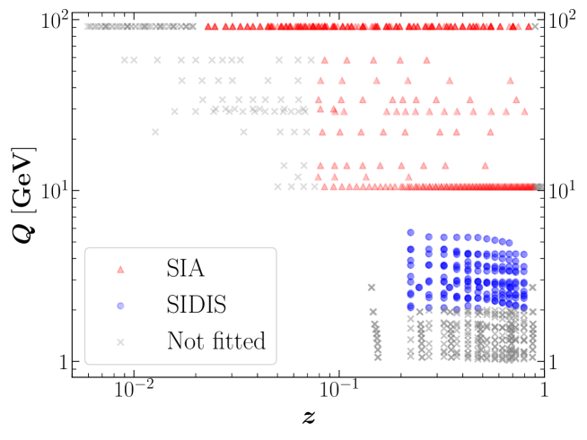
Figure 1: Kinematic coverage in the $(z,Q)$ plane of the data set included in this analysis. Data points are from SIA (red) and SIDIS (blue); gray points are excluded by kinematic cuts.

Kinematic cuts are applied to select only the data points for which perturbative fixed-order predictions are reliable. For SIA, we retain the data points with $z$ in the range $[z_{\rm min},z_{\rm max}]$; the values of $z_{\rm min}$ and $z_{\rm max}$ are chosen as in Ref. [4]: $z_{\rm min}=0.02$ for experiments at a centre-of-mass energy of $M_{Z}$ and $z_{\rm min}=0.075$ for all other experiments; $z_{\rm max}=0.9$ for all experiments. For SIDIS, we retain the data points satisfying $Q>Q_{\rm cut}$, with $Q_{\rm cut}=2$ GeV. This choice maximises the number of data points included in the fit without spoiling its quality and follows from a study of the stability of the fit upon choosing different values of $Q_{\rm cut}$, see Sect. 5.3.3. Overall, after kinematic cuts, we consider $N_{\rm dat}=699$ data points in our baseline fit almost equally split between SIA ($N_{\rm dat}=377$) and SIDIS ($N_{\rm dat}=322$). Each of the two processes is dominated by measurements coming respectively from LEP and $B$-factories, and from COMPASS.

Information on correlations of experimental uncertainties is taken into account whenever available. Specifically, for the BABAR measurement, which is provided with a breakdown of bin-by-bin correlated systematic uncertainties, for the HERMES measurement, which is provided with a set of covariance matrices accounting for correlations of statistical uncertainties obtained from the unfolding procedure, and for the COMPASS measurement, which is provided with a correlated systematic uncertainty. Normalisation uncertainties available for the BELLE, BABAR, TASSO, ALEPH and SLD experiments are assumed to be fully correlated across all data points in each experiment. If the degree of correlation of systematic uncertainties is not known, we sum them in quadrature with the statistical uncertainties. Finally, we symmetrise the systematic uncertainties reported by the BELLE experiment as described in Ref. [36].

3 Theoretical setup

In this section we discuss the theoretical setup used to compute the theoretical predictions for the SIDIS multiplicities corresponding to the measurements performed by COMPASS and HERMES. The computation of SIA cross sections and the evolution of FFs closely follow Refs. [4, 37] and are therefore not discussed here.

We consider the inclusive production of a charged pion, $\pi^{\pm}$, in lepton-nucleon scattering:

$$\ell(k)+N(p)\rightarrow\ell(k^{\prime})+\pi^{\pm}(p_{\pi})+X\,.$$ (1)

The four-momenta involved in this process, along with the definition $q=k-k^{\prime}$, allow one to define the following Lorentz invariants that, under the assumption of a massless target, admit a partonic interpretation:

$$\begin{array}[]{ll}\displaystyle Q^{2}=-q^{2}&\mbox{: (negative) invariant mass of the virtual vector boson,}\\ \\ \displaystyle x=\frac{Q^{2}}{2p\cdot q}&\mbox{: momentum fraction of the nucleon carried by the incoming parton,}\\ \\ \displaystyle z=\frac{p\cdot p_{\pi}}{p\cdot q}&\mbox{: momentum fraction of the outgoing parton carried by the pion,}\\ \\ \displaystyle y=\frac{Q^{2}}{xs}&\mbox{: energy transfer (inelasticity)\,,}\end{array}$$ (2)

with $\sqrt{s}$ being the centre-of-mass energy of the collision. Under the assumption $Q\ll M_{Z}$ (as is the case for all the SIDIS data considered here) only the exchange of a virtual photon can be considered and the triple-differential cross section for the reaction in Eq. (1) can be written as

$$\frac{d^{3}\sigma}{dxdQdz}=\frac{4\pi\alpha^{2}}{xQ^{3}}\left[\left(1+(1-y)^{2}\right)F_{2}(x,z,Q^{2})-y^{2}F_{L}(x,z,Q^{2})\right]\,,$$ (3)

where $\alpha$ is the fine-structure constant, and $F_{2}$ and $F_{L}$ are dimensionless structure functions. Within collinear factorisation, appropriate when $Q\gg\Lambda_{\rm QCD}$, structure functions factorise as

$$\begin{array}[]{rcl}\displaystyle F_{i}(x,z,Q)&=&\displaystyle x\sum_{q\overline{q}}e_{q}^{2}\bigg{\{}\left[C_{i,qq}(x,z,Q)\otimes f_{q}(x,Q)+C_{i,qg}(x,z,Q)\otimes f_{g}(x,Q)\right]\otimes D^{\pi^{\pm}}_{q}(z,Q)\\ &+&\displaystyle\left[C_{i,gq}(x,z,Q)\otimes f_{q}(x,Q)\right]\otimes D^{\pi^{\pm}}_{g}(z,Q)\bigg{\}}\,,\qquad i=2,L\,.\end{array}$$ (4)

The convolution symbol $\otimes$ acts equally on $x$ and $z$ and has to be interpreted as follows:

$$C(x,z)\otimes f(x)\otimes D(z)=\int_{x}^{1}\frac{dx^{\prime}}{x^{\prime}}\int_{z}^{1}\frac{dz^{\prime}}{z^{\prime}}C(x^{\prime},z^{\prime})f\left(\frac{x}{x^{\prime}}\right)D\left(\frac{z}{z^{\prime}}\right)\,.$$ (5)

The sum in Eq. (4) runs over both quark and antiquark flavours active at the scale $Q$, $e_{q}$ is the electric charge of the quark flavour $q$, and $f_{q(g)}$ and $D^{\pi^{\pm}}_{q(g)}$ denote the collinear quark (gluon) PDFs and FFs, respectively. Since in this work we are interested in determining the FFs $D^{\pi^{\pm}}_{q(g)}$ using existing PDFs $f_{q(g)}$, Eq. (4) has been arranged in a way that highlights the role of PDFs as effective charges. Each quark FF contributing to the cross section is weighted by a factor that, thanks to PDFs, depends on the specific flavour or antiflavour. As a consequence, SIDIS cross sections allow for FF quark-flavour separation, a feature that is not present in SIA cross sections where quark and antiquark FFs are always summed with equal weight (see e.g. Eq. (3.1) in Ref. [4]). We use the NNPDF31_nlo_pch_as_0118 [14] as a reference PDF set. In Sect. 4 we will explain how the PDF uncertainty is propagated into SIDIS observables and in Sect. 5.2.2 we will discuss the impact of alternative PDF sets on the determination of FFs.

The coefficient functions $C$ in Eq. (4) admit the usual perturbative expansion

$$C(x,z,Q)=\sum_{n=0}\left(\frac{\alpha_{s}(Q)}{4\pi}\right)^{n}C^{(n)}(x,z)\,,$$ (6)

where $\alpha_{s}$ is the running strong coupling for which we choose $\alpha_{s}(M_{Z})=0.118$ as a reference value. Presently, the full set of coefficient functions for both $F_{2}$ and $F_{L}$ is only known up to $\mathcal{O}(\alpha_{s})$, i.e. NLO [38, 39]. Explicit $x$- and $z$-space expressions up to this order can be found for instance in Ref. [40] and are implemented in the public code APFEL++ [41, 42]. A subset of the $\mathcal{O}(\alpha_{s}^{2})$, i.e. NNLO, corrections has been recently presented in Refs. [43, 44]. However, as long as the full set of $\mathcal{O}(\alpha_{s}^{2})$ corrections are not known, NNLO accuracy cannot be attained. For this reason in this analysis we limit ourselves to NLO accuracy that amounts to considering the first two terms in the sum in Eq. (6). For consistency, also the $\beta$-function and the splitting functions responsible for the evolution of the strong coupling $\alpha_{s}$ and of the FFs, respectively, are computed to NLO accuracy.

So far no heavy-quark mass corrections have been computed for SIDIS. Therefore, our determination of FFs relies on the so-called zero-mass variable-flavour-number scheme (ZM-VFNS). In this scheme all active partons are treated as massless but a partial heavy-quark mass dependence is introduced by requiring that sub-schemes with different numbers of active flavours match at the heavy-quark thresholds. Here we choose $m_{c}=1.51$ GeV and $m_{b}=4.92$ GeV for the charm and bottom thresholds, respectively, as in the NNPDF31_nlo_pch_as_0118 PDF set. In view of the fact that intrinsic heavy-quark FFs play an important role, it is important to stress that in our approach inactive-flavour FFs, such as the charm and bottom FFs below the respective thresholds, are not set to zero. On the contrary, they are allowed to be different from zero but are kept constant in scale below threshold, i.e. they do not evolve. This has the consequence that heavy-quark FFs do contribute to the computation of cross sections also below their threshold. However, in the specific case of SIDIS this contribution is suppressed by the PDFs and only appears at NLO.

A property of the expressions for the perturbative coefficient functions $C$ is that the functions $C^{(n)}(x,z)$ with $n=0,1$ (see Eq. (6)) are bilinear combinations of single-variable functions:

$$C^{(n)}(x,z)=\sum_{t}c_{t}O_{t}^{(1)}(x)O_{t}^{(2)}(z)\,,$$ (7)

where $c_{t}$ are numerical coefficients. This property enables one to decouple the double convolution integral in Eq. (5) into a linear combination of single integrals

$$C^{(n)}(x,z)\otimes f(x)\otimes D(z)=\sum_{t}c_{t}\left[O_{t}^{(1)}(x)\otimes f(x)\right]\left[O_{t}^{(2)}(z)\otimes D(z)\right]\,.$$ (8)

This observation allowed us to considerably speed up the numerical computation of the SIDIS cross sections.

In order to benchmark the implementation in APFEL++ used for the fits and based on the $x$- and $z$-space expressions of Ref. [40], we have carried out a totally independent implementation of the SIDIS cross section based on the Mellin-moment expressions [45, 46]. We made the Mellin-space version of the cross section publicly available through the code MELA [37]. The outcome of the benchmark was totally satisfactory in that in the kinematic region covered by HERMES and COMPASS the agreement between APFEL++ and MELA was well below the per-mil level.

The quantity actually measured by both the HERMES and COMPASS experiments is not an absolute cross section, Eq. (3), but rather an integrated multiplicity defined as

$$\frac{dM}{dz}=\left.\left[\int_{Q_{\rm min}}^{Q_{\rm max}}dQ\int_{x_{\rm min}}^{x_{\rm max}}dx\int_{z_{\rm min}}^{z_{\rm max}}dz\frac{d^{3}\sigma}{dxdQdz}\right]\right/\left[\Delta z\int_{Q_{\rm min}}^{Q_{\rm max}}dQ\int_{x_{\rm min}}^{x_{\rm max}}dx\frac{d^{2}\sigma}{dxdQ}\right]\,,$$ (9)

where the integration bounds define the specific kinematic bin and $\Delta z=z_{\rm max}-z_{\rm min}$. The denominator is given by the DIS cross section inclusive w.r.t. the final state that is thus independent from the FFs. Despite NNLO and heavy-quark mass corrections are known for the inclusive DIS cross sections, we use the ZM-VFNS at NLO also in the denominator of Eq. (9) to match the accuracy of the numerator. However, we have checked that including NNLO and/or heavy-quark mass corrections into the inclusive DIS cross section makes little difference on the determination of FFs.

While the multiplicities measured by the HERMES experiment are binned in the variables $\{x,Q^{2},z\}$, exactly matching the quantity in Eq. (9), those measured by the COMPASS experiment are binned in the variables $\{x,y,z\}$ with $y$ defined in Eq. (2). In this case, theoretical predictions are obtained after adjusting the integration bounds in $Q$ and $x$ in Eq. (9) that become

$$Q_{\rm min}=\sqrt{x_{\rm min}y_{\rm min}s}\,,\qquad Q_{\rm max}=\sqrt{x_{\rm max}y_{\rm max}s}\,,$$ (10)

and

$$x_{\rm min}\rightarrow{\rm max}\left[x_{\rm min},\frac{Q^{2}}{sy_{\rm max}}\right]\qquad x_{\rm max}\rightarrow{\rm min}\left[x_{\rm max},\frac{Q^{2}}{sy_{\rm min}}\right]\,,$$ (11)

with $y_{\rm min}$ and $y_{\rm max}$ the bin bounds in $y$. Moreover, both HERMES and COMPASS measure cross sections within a specific fiducial region given by

$$W=\sqrt{\frac{(1-x)Q^{2}}{x}}\geq W_{\rm low}\,,\quad y_{\rm low}\leq y\leq y_{\rm up}\,,$$ (12)

with the values of $W_{\rm low}$, $y_{\rm low}$, and $y_{\rm up}$ reported in Tab. 1. These constraints reduce the phase space of some bins placed at the edge of the fiducial region. The net effect is that of replacing the $x$ integration bounds in Eq. (9) with

$$x_{\rm min}\rightarrow\overline{x}_{\rm min}={\rm max}\left[x_{\rm min},\frac{Q^{2}}{sy_{\rm up}}\right]\quad\mbox{and}\quad x_{\rm max}\rightarrow\overline{x}_{\rm max}={\rm min}\left[x_{\rm max},\frac{Q^{2}}{sy_{\rm low}},\frac{Q^{2}}{Q^{2}+W_{\rm low}^{2}}\right]\,,$$ (13)

with $x_{\rm min}$ and $x_{\rm max}$ to be interpreted as in Eq. (11) in the case of COMPASS. We stress that in our determination of FFs all the integrals in Eq. (9) are duly computed during the fit. The effect of computing these integrals, in comparison to evaluating the cross sections at the central point of the bins, is modest for COMPASS but sizeable for HERMES. However, in both cases the integration contributes to achieving a better description of the data.

Both the HERMES and COMPASS experiments measure multiplicities for $\pi^{+}$ and $\pi^{-}$ separately. However, $\pi^{+}$ and $\pi^{-}$ are related by charge conjugation. In practice, this means that it is possible to obtain one from the other by exchanging quark and antiquark distributions and leaving the gluon unchanged:

$$D_{q(\overline{q})}^{\pi^{-}}(x,Q)=D_{\overline{q}(q)}^{\pi^{+}}(x,Q)\,,\quad D_{g}^{\pi^{-}}(x,Q)=D_{g}^{\pi^{+}}(x,Q)\,.$$ (14)

In this analysis, we use this symmetry to express the $\pi^{-}$ FFs in terms of the $\pi^{+}$ ones and effectively only extract the latter.

We finally note that part of the HERMES measurements and all of the COMPASS ones are performed on isoscalar targets (deuterium for HERMES and lithium for COMPASS, see Table 1). To account for this we have adjusted the PDFs of the target by using SU(2) isospin symmetry to deduce the neutron PDFs from the proton ones, which simply amounts to exchanging (anti) up and (anti) down PDFs, and taking the average between proton and neutron PDFs. No nuclear corrections are taken into account; no target mass corrections are considered either, given the complexity to consistently account for them together with final-state hadron mass corrections [47].

4 Methodology

The statistical framework that we adopted for the inference of the MAPFF1.0 FFs from experimental data relies on the Monte Carlo sampling method that is nowadays widely used in QCD analyses [14, 15, 17, 18, 4, 19, 48, 7, 9, 49, 50, 51]. The main assumption is that the data originates from a multivariate Gaussian distribution

$$\mathcal{G}\left(\bm{x}^{(k)}\right)\propto\exp{\left[\left(\bm{x}^{(k)}-\bm{\mu}\right)^{T}\cdot\bm{C}^{-1}\cdot\left(\bm{x}^{(k)}-\bm{\mu}\right)\right]}\,,$$ (15)

where $\bm{x}^{(k)}=\{x_{1}^{(k)},x_{2}^{(k)},\dddot{},x^{(k)}_{N_{\text{dat}}}\}$ are equally probable replicas, $k=1,\dots,N_{\rm rep}$, of a set of $N_{\text{dat}}$ measured quantities. The expectation value of the distribution corresponding to the measured data is $\bm{\mu}=\{\mu_{1},\,\mu_{2},\,\dddot{},\mu_{N_{\text{dat}}}\}$ and $\bm{C}$ is the covariance matrix that encodes all sources of uncertainties. The elements of the covariance matrix are defined as follows:

$$C_{ij}=\delta_{ij}\sigma_{i,\,\text{unc}}^{2}+\sum_{\beta}\sigma^{(\beta)}_{i,\,\text{corr}}\sigma^{(\beta)}_{j,\,\text{corr}}\,,$$ (16)

where $\sigma_{i,\,\text{unc}}$ denotes the sum in quadrature of all uncorrelated uncertainties associated to the $i$-th point and $\sigma^{(\beta)}_{i,\,\text{corr}}$ is the correlated uncertainty of source $\beta$ associated to the same point.

The Monte Carlo method aims at propagating the experimental uncertainties into the space of parameters defined in our case by a neural network. In order to do so, we generate $N_{\text{rep}}$ replicas of the data, $\bm{x}^{(k)}$, using the Cholesky decomposition $\bm{L}$ of the covariance matrix $\bm{C}$ ($\bm{C}=\bm{L}\cdot\bm{L}^{T}$) so that

$$\bm{x}^{(k)}=\bm{\mu}+\bm{L}\cdot\bm{r^{(k)}}\,,$$ (17)

where $\bm{r}^{(k)}$ is an $N_{\text{dat}}$-dimensional normal random vector such that the full set of replicas satisfies

$$\frac{1}{N_{\text{rep}}}{\displaystyle\sum^{N_{\text{rep}}}_{k}x_{i}^{(k)}}\simeq\mu_{i}\,,\qquad\frac{1}{N_{\text{rep}}}{\displaystyle\sum^{N_{\text{rep}}}_{k}x_{i}^{(k)}x_{j}^{(k)}}\simeq\mu_{i}\mu_{j}+C_{ij}\,,$$ (18)

in the limit of a sufficiently large number of replicas. We have verified that the choice $N_{\rm rep}=200$ satisfies Eq. (18) with sub-percent accuracy. In the case of SIDIS, a different proton PDF replica taken at random from the NNPDF31_nlo_pch_as_0118 set is associated to each replica $\bm{x}^{(k)}$. This ensures the propagation of PDF uncertainty into the FF uncertainty.

In order to choose the best set of independent FF combinations entering our parametrisation basis, we study three different cases.

1. 11 independent flavours. This is the most general case implied by Eq. (4) where one aims at disentangling all FF flavours and the gluon FF. This parametrisation is overly redundant in that the data set used is not able to constrain all 11 combinations.

2. 7 independent flavours. The sea distributions are assumed to be partially symmetric. Specifically, $D^{\pi^{+}}_{q}=D^{\pi^{+}}_{\bar{q}}$, for $q=s,c,b$, and $D^{\pi^{+}}_{d}=D^{\pi^{+}}_{\bar{u}}$. By doing so, we reduce the number of independent distributions down to 7. We observe that under these assumptions the quality of the fit does not significantly deteriorate with respect to the most general case discussed above. In particular, we find it to be the best solution in terms of generality and accuracy and therefore we adopt it as our baseline parametrisation.

3. 6 independent flavours. The approximate SU(2) isospin symmetry would suggest that the additional constraint $D^{\pi^{+}}_{u}=D^{\pi^{+}}_{\bar{d}}$ may hold, further lowering the number of independent combinations down to 6. However, it turns out that this additional assumption leads to a deterioration of the quality of the fit therefore we dropped it.

Finally, the set of 7 independent FF combinations parametrised in our fit are:

$$\{D^{\pi^{+}}_{u},\quad D^{\pi^{+}}_{\bar{d}},\quad D^{\pi^{+}}_{d}=D^{\pi^{+}}_{\bar{u}},\quad D^{\pi^{+}}_{s}=D^{\pi^{+}}_{\bar{s}},\quad D^{\pi^{+}}_{c}=D^{\pi^{+}}_{\bar{c}},\quad D^{\pi^{+}}_{b}=D^{\pi^{+}}_{\bar{b}},\quad D^{\pi^{+}}_{g}\}\,.$$ (19)

The parametrisation is introduced at the initial scale $\mu_{0}=5\,\text{GeV}$ and consists of a single one-layered feed-forward neural network $\mathcal{N}_{i}(z;\bm{\theta})$, where $\bm{\theta}$ denotes the set of parameters. This network has one input node corresponding to the momentum fraction $z$, 20 intermediate nodes with a sigmoid activation function, and 7 output nodes with a linear activation function corresponding to the flavour combinations in Eq. (19). This architecture $[1,\,20,\,7]$ amounts to a total of 187 free parameters. We do not include any power-like function to control the low- and high-$z$ behaviours, however we do impose the kinematic constraint $D_{i}^{\pi^{+}}(z=1)=0$ by simply subtracting the neural network itself at $z=1$ as done in Ref. [4]. Moreover, we constrain the FFs to be positive-definite by squaring the outputs. This choice is motivated by the fact that allowing for negative distributions leads to FFs that may become unphysically negative. Our parametrisation finally reads

$$zD^{\pi^{+}}_{i}(z,\mu_{0}=5\,\text{GeV})=\Big{(}\mathcal{N}_{i}(z;\bm{\theta})-\mathcal{N}_{i}(1;\bm{\theta})\Big{)}^{2}\,,$$ (20)

where the index $i$ runs over the combinations in Eq. (19).

The fit is performed by maximising the log-likelihood $\mathcal{L}\left(\bm{\theta}|\bm{x}^{(k)}\right)$, which is the probability of observing a given data replica $\bm{x}^{(k)}$ given the set of parameters $\bm{\theta}^{(k)}$. Together with the multivariate Gaussian assumption, this is equivalent to minimising the $\chi^{2}$. This is defined as

$$\chi^{2(k)}\equiv\left(\bm{T}(\bm{\theta}^{(k)})-\bm{x}^{(k)}\right)^{T}\cdot\bm{C}^{-1}\cdot\left(\bm{T}(\bm{\theta}^{(k)})-\bm{x}^{(k)}\right)\,,$$ (21)

where $\bm{T}(\bm{\theta}^{(k)})$ is the set of theoretical predictions with the neural-network parametrisation as input. We set $T_{i}(\bm{\theta}^{(k)})=\mu_{i}$ if point $i$ does not satisfy the kinematic cuts defined in Sect. 3 or if it belongs to the validation set.

We adopt the cross-validation procedure in order to avoid overfitting our FFs. For each data replica, data sets amounting to more than 10 data points are randomly split into training and validation subsets, each containing half of the points, and only those in the training set are used in the fit. Data sets with 10 or less data points are instead fully included in the training set. The $\chi^{2}$ of the validation set is monitored during the minimisation of the training $\chi^{2}$ and the fit is stopped when the validation $\chi^{2}$ reaches its absolute minimum. Replicas whose total $\chi^{2}$ per point, i.e. the $\chi^{2}$ computed over all data points in the fit, is larger than 3 are discarded.

The minimisation algorithm adopted for our fit is a trust-region algorithm, specifically the Levenberg-Marquardt algorithm as implemented in the Ceres Solver code [52]. This is an open source C++ library for modelling and solving large optimisation problems. The neural-network parametrisation and its analytical derivatives with respect to the free parameters are provided by NNAD [20], an open source C++ library that provides a fast implementation of an arbitrarily large feed-forward neural network and its analytical derivatives.

5 The MAPFF1.0 set

In this section we present the main results of this analysis. In Sect. 5.1 we discuss the quality of our baseline fit that we dub MAPFF1.0. In Sect. 5.2 we illustrate its features: we compare our FFs to other recent determinations and we study the stability of the fit upon the choice of input PDFs and of the parametrisation scale $\mu_{0}$. In Sect. 5.3 we study the impact of some specific data sets: we discuss the origin of the difficulty in fitting SIA charm-tagged data, we investigate the impact of the SIDIS data on FFs, and finally we study the dependence of the fit quality on the low-$Q$ cut on the SIDIS data.

5.1 Fit quality

Tab. 2 reports the value of the $\chi^{2}$ per data point for the individual data sets included in the MAPFF1.0 fit along with the number of data points $N_{\rm dat}$ that pass the kinematic cuts discussed in Sect. 2. The table also reports the partial $\chi^{2}$ values of the SIDIS and SIA data sets separately as well as the global one.

Experiment	$\chi^{2}$ per point	$N_{\rm dat}$ after cuts
HERMES $\pi^{-}$ deuteron	0.60	2
HERMES $\pi^{-}$ proton	0.02	2
HERMES $\pi^{+}$ deuteron	0.30	2
HERMES $\pi^{+}$ proton	0.53	2
COMPASS $\pi^{-}$	0.80	157
COMPASS $\pi^{+}$	1.07	157
Total SIDIS	0.78	322
BELLE $\pi^{\pm}$	0.09	70
BABAR prompt $\pi^{\pm}$	0.90	39
TASSO 12 GeV $\pi^{\pm}$	0.97	4
TASSO 14 GeV $\pi^{\pm}$	1.39	9
TASSO 22 GeV $\pi^{\pm}$	1.85	8
TPC $\pi^{\pm}$	0.22	13
TASSO 30 GeV $\pi^{\pm}$	0.34	2
TASSO 34 GeV $\pi^{\pm}$	1.20	9
TASSO 44 GeV $\pi^{\pm}$	1.20	6
TOPAZ $\pi^{\pm}$	0.28	5
ALEPH $\pi^{\pm}$	1.29	23
DELPHI total $\pi^{\pm}$	1.29	21
DELPHI $uds$ $\pi^{\pm}$	2.84	21
DELPHI bottom $\pi^{\pm}$	1.67	21
OPAL $\pi^{\pm}$	1.72	24
SLD total $\pi^{\pm}$	1.14	34
SLD $uds$ $\pi^{\pm}$	2.05	34
SLD bottom $\pi^{\pm}$	0.55	34
Total SIA	1.10	377
Global data set	0.90	699

Table 2: Values of the $\chi^{2}$ per data point for the individual data sets included in the MAPFF1.0 analysis. The number of data points $N_{\rm dat}$ that pass kinematic cuts and the SIDIS, SIA, and global $\chi^{2}$ values are also displayed.

The global $\chi^{2}$ per data point, equal to 0.90, indicates a general very good description of the entire data set. A comparable fit quality is observed for both the SIDIS and SIA sets separately, with collective $\chi^{2}$ values equal to 0.78 and 1.10, respectively. A closer inspection of Tab. 2 reveals that an acceptable description is achieved for all of the individual data sets. Some particularly small $\chi^{2}$ values are also obtained. This is the case of the HERMES $\pi^{-}$ and BELLE data. In the case of HERMES, the smallness of the $\chi^{2}$ is not statistically significant given that only two data points survive the cuts. The smallness of the $\chi^{2}$ of BELLE is instead well-known and follows from an overestimate of the systematic uncertainties [2, 53, 4, 54].

It is instructive to look at the comparison between data and predictions obtained with the MAPFF1.0 FFs for some selected data sets. The top row of Fig. 2 shows the comparison for the $B$-factory experiments BELLE and BABAR at $\sqrt{s}\simeq 10.5$ GeV, while the bottom row shows the comparison for two representative data sets at $\sqrt{s}=M_{Z}$, i.e. the total cross sections from DELPHI and SLD. The upper panels display the absolute distributions while the lower ones the ratio to the experimental central values. The shaded areas indicate the regions excluded from the fit by the kinematic cuts. In order to facilitate the visual comparison, predictions are shifted to account for correlated systematic uncertainties [55], when present. Consistently with the $\chi^{2}$ values reported in Tab. 2, the description of these data sets is very good within cuts.

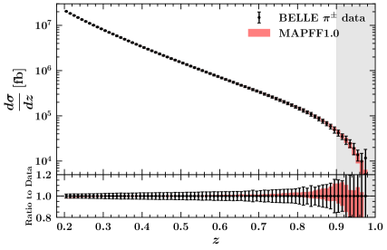
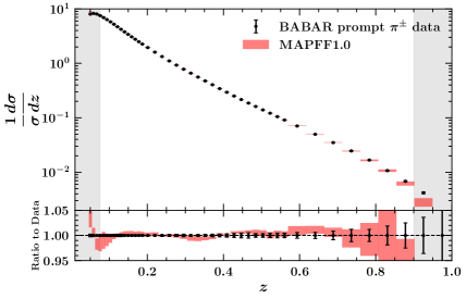
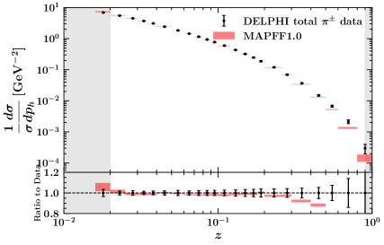
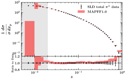
Figure 2: Top row: data-theory comparison for the $B$-factory experiments BELLE (left) and BABAR (right) at $\sqrt{s}\simeq 10.5$ GeV. Bottom row: representative data-theory comparison for SIA data sets at $\sqrt{s}=M_{Z}$ from DELPHI (left) and SLD (right). The shaded regions are excluded from the fit.

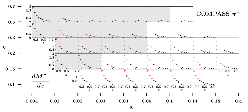
Figure 3: Data-theory comparison for the $\pi^{-}$ multiplicities from COMPASS. The shaded bins are excluded from the fit due to the cut in $Q$.

Fig. 3 shows the data-theory comparison for the COMPASS $\pi^{-}$ multiplicities. Each panel displays a distribution in $z$ corresponding to a bin in $x$ and $y$. As above, theoretical predictions have been shifted to ease the visual comparison. The grey-shaded panels are not fitted because they do not fulfil the cut in $Q$ discussed in Sect. 2. Once again, the goodness of the $\chi^{2}$ values in Tab. 2 is reflected in a general very good description of the data. The analogous plot for $\pi^{+}$ multiplicities looks qualitatively similar to Fig. 3, therefore it is not shown.

5.2 Fragmentation Functions

We now present our FFs. We first compare them with other FF sets, then we study the impact of some relevant theoretical choices.

5.2.1 Comparison with other FF sets

In Fig. 4 we compare the $\pi^{+}$ FFs obtained from our baseline fit, MAPFF1.0, to those from JAM20 [6] and DEHSS14 [2]. All three sets include a similar SIA and SIDIS data set. However, the JAM20 set also includes inclusive deep-inelastic scattering and fixed-target Drell-Yan measurements that are used to simultaneously determine PDFs, while the DEHSS14 set also includes pion production measurements in proton-proton collisions.

In the case of $D_{u}^{\pi^{+}}$ and $D_{\bar{d}}^{\pi^{+}}$, as is clear from the upper row of Fig. 4, JAM20 assumes SU(2) isospin symmetry which results in $D_{u}^{\pi^{+}}=D_{\bar{d}}^{\pi^{+}}$. DEHSS14 instead assumes $D_{u}^{\pi^{+}}+D_{\bar{u}}^{\pi^{+}}\propto D_{{d}}^{\pi^{+}}+D_{\bar{d}}^{\pi^{+}}$ where the proportionality factor is a $z$-independent constant that parameterises any possible isospin symmetry violation. As explained in Sect. 4, in MAPFF1.0 we parametrise $D_{u}^{\pi^{+}}$ and $D_{\bar{d}}^{\pi^{+}}$ independently, thus allowing for a $z$-dependent isospin symmetry violation which however turned out not to be significant. For $z\lesssim 0.1$, where experimental data is sparse (see Fig. 1), the relative uncertainty on the $D_{u}^{\pi^{+}}$ and $D_{\bar{d}}^{\pi^{+}}$ distributions from MAPFF1.0 is larger than that of the corresponding distributions from DEHSS14 and JAM20. At large $z$, we observe a suppression of the MAPFF1.0 FFs w.r.t. DEHSS14 and JAM20 for both $D_{u}^{\pi^{+}}$ and $D_{\bar{d}}^{\pi^{+}}$. This suppression is compensated by an enhancement of the sea quarks as we will further discuss below.

Figure 4: Comparison of the MAPFF1.0, DEHSS14 [2], and JAM20 [6] FFs. We display the $D_{u}^{\pi^{+}}$, $D_{\bar{d}}^{\pi^{+}}$, $D_{\bar{u}}^{\pi^{+}}$, $D_{s^{+}}^{\pi^{+}}$, $D_{c^{+}}^{\pi^{+}}$, $D_{b^{+}}^{\pi^{+}}$, $D_{u^{+}+d^{+}+s^{+}}^{\pi^{+}}$ and $D_{g}^{\pi^{+}}$ FFs at $\mu=5$ GeV. For each FF we plot the absolute distributions in the upper panel and their ratio to the central value of the MAPFF1.0 set in the lower one.

In the case of the sea FFs, we find a good agreement at very large $z$ with both DEHSS14 and JAM20 for $D_{s^{+}}^{\pi^{+}}$ and $D_{b^{+}}^{\pi^{+}}$. At low $z$, on the one hand, we observe that the sea FFs from DEHSS14, except $D_{\bar{u}}^{\pi^{+}}$, and the $D_{s^{+}}^{\pi^{+}}$ FF from JAM20 are within the MAPFF1.0 uncertainties. On the other hand, JAM20 and DEHSS14 show an enhancement for the rest of the FFs w.r.t. MAPFF1.0.

We note that a very good agreement at intermediate $z$ is found for the light singlet $D_{u^{+}}^{\pi^{+}}+D_{d^{+}}^{\pi^{+}}+D_{s^{+}}^{\pi^{+}}$ combination. This particular combination is most sensitive to inclusive SIA data and the agreement reflects the fact that all three collaborations are able to describe this data comparably well. The gluon FF of MAPFF1.0 is affected by large uncertainties. This is a consequence of using observables that are not directly sensitive to this distribution. The MAPFF1.0, JAM20, and DEHSS14 gluon FFs remain fairly compatible within uncertainties.

Finally, we observe that most of the distributions of the MAPFF1.0 set present a turn-over in the region $0.1\lesssim z\lesssim 0.2$ that is absent in the other two sets. This feature can be ascribed to the fact that MAPFF1.0 implements cuts on the minimum value of $z$ that are generally lower than those used by the other two collaborations (see Ref. [4] for a detailed study).

5.2.2 Impact of theoretical choices

We have studied the stability of our FFs upon the input PDF set used to compute SIDIS multiplicities. In order to assess the impact of the PDF uncertainty, we performed an additional fit using the central PDF member of the NNPDF31_nlo_pch_as_0118 set for all Monte Carlo replicas. We found that neglecting the PDF uncertainty has a very small impact on the FFs. In addition, we studied the dependence of the FFs on the specific PDF set by performing two additional fits using the central member of the CT18NLO [56] and MSHT20nlo_as118 [57] sets. Also in this case, we found that the difference at the level of FFs was very mild. In fact, a reduced sensitivity to the treatment of PDFs was to be expected because our FFs depend on them only through the SIDIS measurements that are delivered as multiplicities for both by COMPASS and HERMES. For this particular observable, see Eq. (9), PDFs enter both the numerator and the denominator, hence the sensitivity of the observable to the PDFs largely cancels out.

We have also studied the stability of our FFs upon the choice of the parametrisation scale $\mu_{0}$. To this purpose, we have repeated our baseline fit by lowering the value of $\mu_{0}$ from 5 GeV to 1 GeV. This led to almost identical FFs. We stress that the possibility to freely choose the parameterisation scale, no matter whether above or below the heavy quark thresholds, is due to the fact that we do not set inactive-flavour FFs to zero below their respective threshold (see Sect. 3).

5.3 Impact of the data

We now justify our exclusion of the SIA charm-tagged data from the fit as well as our choice of the cut on the virtuality $Q^{2}$ for the SIDIS data. We also discuss the separate impact of COMPASS and HERMES on the FFs.

5.3.1 Data compatibility

As mentioned in Sect. 2, we did not include the SLD charm-tagged measurements because we have not been able to achieve an acceptable description for this particular data set. Specifically, we found that its inclusion causes a general deterioration of the fit quality with a $\chi^{2}$ per data point of SLD-charm itself exceeding 6. We have identified the origin of this behaviour in an apparent tension between the SLD charm-tagged and the COMPASS measurements. As a matter of fact, if the COMPASS data is excluded from the fit, the SLD charm-tagged data can be satisfactorily fitted. More precisely we observe that the inclusion of COMPASS on top of SIA data leads to a suppression of the $D_{u^{+}}^{\pi^{+}+\pi^{-}}=D_{u}^{\pi^{+}}+D_{\bar{u}}^{\pi^{+}}+D_{u}^{\pi^{-}}+D_{\bar{u}}^{\pi^{-}}$ distribution for $z\gtrsim 0.1$ as compared to a fit to SIA data only. This behaviour is visible in the left panel of Fig. 5 where the $D_{u^{+}}^{\pi^{+}+\pi^{-}}$ distribution for the sum of positively and negatively charged pions is displayed at $\mu=5$ GeV for the following FF sets: the baseline MAPFF1.0 fit (which includes SIA and SIDIS data), a MAPFF1.0-like fit to SIA data only, and the NNFF1.0 fit [4] (which includes SIA data only). We see that at intermediate values of $z$ the SIA-only MAPFF1.0 fit and NNFF1.0 fit are in good agreement, while the baseline MAPFF1.0 fit is suppressed. As a consequence of this suppression, the $D_{c^{+}}^{\pi^{+}+\pi^{-}}=D_{c}^{\pi^{+}}+D_{\bar{c}}^{\pi^{+}}+D_{c}^{\pi^{-}}+D_{\bar{c}}^{\pi^{-}}$ distribution of the global MAPFF1.0 fit gets enhanced to accommodate the inclusive SIA data. This effect is visible in the right panel of Fig. 5 that shows for the $D_{c^{+}}^{\pi^{+}+\pi^{-}}$ distribution a good agreement between the SIA-only fit and NNFF1.0 with the global MAPFF1.0 fit being generally harder for $z\gtrsim 0.1$. This enhancement of the $D_{c^{+}}^{\pi^{+}+\pi^{-}}$ distribution deteriorates the description of the SLD charm-tagged data. This is not surprising in that charm-tagged observables are naturally sensitive to the charm FFs. We interpret the suppression of $D_{u^{+}}^{\pi^{+}+\pi^{-}}$ and the consequent enhancement of $D_{c^{+}}^{\pi^{+}+\pi^{-}}$ as an effect of the COMPASS data. We conclude that the COMPASS and SLD charm-tagged data are in tension and we decided to keep the former and drop the latter from our global fit.

We finally note that the suppression of the $D_{u^{+}}^{\pi^{+}+\pi^{-}}$ distribution also leads to a deterioration of the description of the $uds$-tagged measurements from both DELPHI and SLD that feature a $\chi^{2}$ per data point of respectively 2.84 and 2.05 (see Tab. 2). However, this deterioration is milder than that of the SLD charm-tagged data, thus we opted for keeping the $uds$-tagged measurements in the fit.

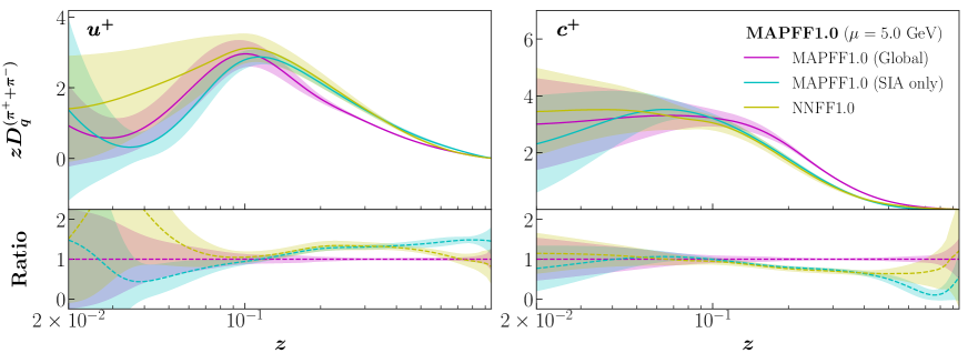
Figure 5: Comparison between the baseline MAPFF1.0 fit (which includes SIA and SIDIS data), a variant of the MAPFF1.0 fit to SIA data only, and NNFF1.0 [4] (which includes only SIA data). The left (right) plot shows the $D_{u^{+}}^{\pi^{+}+\pi^{-}}$ ($D_{c^{+}}^{\pi^{+}+\pi^{-}}$) distribution at $\mu=5$ GeV. The upper panels display the absolute distributions while the lower ones their ratio to the central value of the baseline MAPFF1.0 fit.

5.3.2 Impact of SIDIS data

In this section, we study the impact of the individual SIDIS data sets included in our analysis. To this purpose we have repeated our baseline fit by removing either the COMPASS or the HERMES measurements. The three fits are compared in Fig. 6.

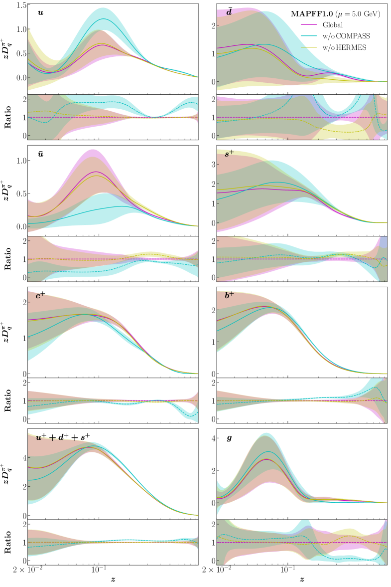
Figure 6: Comparison between three variant of the MAPFF1.0 fit: a fit to the global data set, a fit without the COMPASS data, and a fit without the HERMES data. The format of the plot is as in Fig. 4.

We note that the number of data points that survive the kinematic cuts defined in Sect. 2 is 8 for HERMES and 314 for COMPASS. Despite the limited amount of data points, HERMES still provides a sizeable constraint in the region of its coverage. As shown in Fig. 6 the impact of the HERMES data in the region $0.2\lesssim z\lesssim 0.6$ can be summarised as follows:

• Overruling the COMPASS data for $D_{\bar{d}}^{\pi^{+}}$ and partly for $D_{\bar{u}}^{\pi^{+}}$. When excluding HERMES, these FFs are respectively suppressed by approximately 2-$\sigma$ and enhanced by 1-$\sigma$.

• Competing with the COMPASS data for $D_{s^{+}}^{\pi^{+}}$ because both datasets have a comparable impact on this FF combination.

• Overruled by the COMPASS data for the remaining FFs, namely $D_{u}^{\pi^{+}}$, $D_{c^{+}}^{\pi^{+}}$, $D_{b^{+}}^{\pi^{+}}$, $D_{g}^{\pi^{+}}$ and for the combination $D_{u^{+}+d^{+}+s^{+}}^{\pi^{+}}$, as their trend in the global fit follows that of the fit without HERMES.

We finally note that, as expected, the three fits display a similar behaviour in the extrapolation regions for both the central value and the uncertainty.

5.3.3 Impact of SIDIS energy scale kinematic cut

As discussed in Sect. 2, we included in our fit only SIDIS data whose value of $Q$ is larger than $Q_{\rm cut}=2$ GeV. The reason for excluding low-energy data stems from the fact that, as $Q$ decreases, higher-order perturbative corrections become increasingly sizeable until eventually predictions based on NLO calculations become unreliable. Therefore, $Q_{\rm cut}$ has to be such that NLO accuracy provides an acceptable description of the data included in the fit.

Our particular choice is informed by studying the dependence of the fit quality on the value of $Q_{\rm cut}$. To this purpose, we have repeated our baseline analysis by varying the value of $Q_{\rm cut}$ in the range $[1.00,2.50]$ GeV. Fig. 7 shows the behaviour of the $\chi^{2}$ per data point for HERMES, COMPASS, and for the total data set as functions of $Q_{\rm cut}$. For each point in $Q_{\rm cut}$ the number of data points surviving the cut is also displayed. As expected, the $\chi^{2}$ is a decreasing function of $Q_{\rm cut}$ confirming the fact that perturbation theory works better for larger values of the hard scale $Q$. However, while HERMES can be satisfactorily described down to $Q_{\rm cut}=1$ GeV with a $\chi^{2}$ that never exceeds one, the COMPASS $\chi^{2}$ quickly deteriorates reaching a value as large as 3.5 at $Q_{\rm cut}=1$ GeV. Given the large size of the COMPASS data set, this deterioration drives the total $\chi^{2}$ that also becomes significantly worse as $Q_{\rm cut}$ decreases. Based on Fig. 7, we have chosen $Q_{\rm cut}=2$ GeV for our baseline fit because it guarantees an appropriate description not only of the COMPASS data, but also of the entire data set.

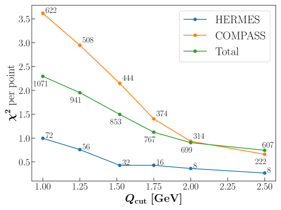
Figure 7: Behaviour of the $\chi^{2}$ per data point as a function of the cut on $Q$, $Q_{\rm cut}$, applied to the SIDIS data. The $\chi^{2}$ is computed for the total MAPFF1.0 data set (green curve), for the COMPASS data set (orange curve), and for the HERMES data set (blue curve). For each value of $Q_{\rm cut}$ considered, the plot also displays the number of data points $N_{\rm dat}$ that pass the cut.

6 Summary and outlook

In this paper we have presented a determination of the collinear FFs of charged pions, dubbed MAPFF1.0, based on a broad data set that includes SIA and SIDIS data. Experimental uncertainties are consistently treated by taking into proper account correlations whenever available and propagated into the fitted FFs using the Monte Carlo sampling method. Theoretical predictions are computed to NLO accuracy in perturbative QCD and duly integrated over the relevant final phase space when required in order to closely match the experimental data. Appropriate kinematic cuts aimed at ensuring the validity of the theoretical predictions for the fitted data have also been enforced. Seven independent combinations of FFs are parametrised in terms of a single neural network and fitted to data by means of a trust-region algorithm making use of the knowledge of the analytic derivatives of the neural network itself. The global $\chi^{2}$ as well as the $\chi^{2}$ of all the single data sets included in the fits are fully satisfactory. This is naturally reflected in a very good match between experimental data included in the fit and the corresponding theoretical predictions. We have compared the resulting MAPFF1.0 FF set to two other recent determinations, DEHSS14 and JAM20, finding some noticeable difference especially at the level of the uncertainties.

In order to assess the stability and robustness of our results, we have performed a number of variations w.r.t. the baseline settings.

As discussed in Sect. 4, we have explored different numbers of independent FF combinations and selected the one that implies a minimal set of restrictions in order to avoid any bias deriving from too restrictive flavour assumptions. This resulted in a set of 7 positive-definite independent combinations fitted to data.

Given the dependence of the SIDIS predictions on PDFs, in Sect. 5.2.2 we have discussed the effect on FFs of including the PDF uncertainty as well as that of using different PDF sets. As expected on the basis of the particular structure of the SIDIS observable being fitted (multiplicities), we found that the resulting FFs are almost insensitive to the treatment of PDFs both in terms of uncertainties and central values.

In Sect. 5.3.1 we showed that the inclusion of SIDIS data on top of the SIA data sets has the effect of “rebalancing” the total up and total charm FFs with the consequence of substantially worsening the description of SLD charm-tagged data. As a consequence, the SLD charm-tagged data set has been excluded from the analysis.

In Sect. 5.3.2 we have studied the interplay between SIA and SIDIS data and observed that the latter, mostly represented by COMPASS, plays a vital role in constraining and separating FFs flavours. However, we also noticed that HERMES, despite the limited number of points, has a noticeable impact on FFs.

Finally, in Sect. 5.3.3 we have justified our particular choice for the cut on the minimum value of $Q$, $Q_{\rm cut}=2$ GeV, for the SIDIS data included in the fit. We argued that this particular value guarantees a reliable applicability of NLO accurate predictions to the SIDIS data set. As a matter of fact, $Q_{\rm cut}=2$ GeV allows us to obtain a global $\chi^{2}$ as well as the $\chi^{2}$ of the COMPASS data set that are close to unity.

A possible natural continuation to this work is a determination of the charged kaon, proton/antiproton and charged unidentified hadron FFs. In all these cases, SIA and SIDIS data is available that would allow for an extraction of these sets of distributions in a very similar manner as done here for pions. In this respect, particularly interesting is the measurement of the $K^{-}/K^{+}$ and $p/\overline{p}$ ratios recently presented by COMPASS [58, 59]. These observables are affected by very small systematic uncertainties and are thus promising to constrain kaon and proton FFs.

In this work we have exploited the complementarity of SIA and SIDIS observables to obtain and accurate determination and separation of the quark FFs of the pion. However, both SIA and SIDIS are poorly sensitive to the gluon FF because in both cases gluon-initiated channels are only present starting from NLO. This is reflected in a relatively large uncertainty of this distribution (see for example Fig. 4). In order to constrain the gluon FF, we plan to use data for single-pion production in proton-proton collisions. As proven in Ref. [19], this process is directly sensitive to the gluon FF already at LO thus providing an effective handle on this distribution.

Finally, we point out that an accurate determination of the collinear FFs of the pions (as well as that of other light hadrons such as the kaons and the protons) is instrumental to a reliable determination of transverse-momentum-dependent (TMD) distributions. Specifically, the description of $p_{\rm T}$-dependent SIDIS multiplicities at low values of $p_{\rm T}$, where $p_{\rm T}$ is the transverse momentum of the outgoing hadron, can be expressed in terms of TMD PDFs and TMD FFs that in turn depend on their collinear counterpart. The HERMES [33] and COMPASS [60] experiments have measured this observable. This data can then be used to extract TMD distributions extending, for example, the analysis of TMD PDFs carried out in Ref. [61] to the TMD FFs relying on the collinear FFs determined in this work. This goal will be pursued by the MAP Collaboration in the future.

The entirety of the results presented in this paper have been obtained using the public code available from:

https://github.com/MapCollaboration/MontBlanc.

On this website it is possible to find some documentation concerning the code usage as well as the FF sets in the LHAPDF format. We provide three sets of FFs with $N_{\rm rep}=200$ replicas each and of their average for the positively and negatively charged pions and for their sum. These are correspondingly called MAPFF10NLOPIp, MAPFF10NLOPIm, and MAPFF10NLOPIsum and are made available via the LHAPDF interface [62] at:

https://lhapdf.hepforge.org/.

References

- [1] A. Metz and A. Vossen, Parton Fragmentation Functions, Prog. Part. Nucl. Phys. 91 (2016) 136–202, [arXiv:1607.02521].
- [2] D. de Florian, R. Sassot, M. Epele, R. J. Hernández-Pinto, and M. Stratmann, Parton-to-Pion Fragmentation Reloaded, Phys. Rev. D 91 (2015), no. 1 014035, [arXiv:1410.6027].
- [3] D. P. Anderle, F. Ringer, and M. Stratmann, Fragmentation Functions at Next-to-Next-to-Leading Order Accuracy, Phys. Rev. D 92 (2015), no. 11 114017, [arXiv:1510.05845].
- [4] NNPDF Collaboration, V. Bertone, S. Carrazza, N. P. Hartland, E. R. Nocera, and J. Rojo, A determination of the fragmentation functions of pions, kaons, and protons with faithful uncertainties, Eur. Phys. J. C 77 (2017), no. 8 516, [arXiv:1706.07049].
- [5] D. P. Anderle, T. Kaufmann, M. Stratmann, and F. Ringer, Fragmentation Functions Beyond Fixed Order Accuracy, Phys. Rev. D 95 (2017), no. 5 054003, [arXiv:1611.03371].
- [6] E. Moffat, W. Melnitchouk, T. Rogers, and N. Sato, Simultaneous Monte Carlo analysis of parton densities and fragmentation functions, arXiv:2101.04664.
- [7] N. Sato, J. J. Ethier, W. Melnitchouk, M. Hirai, S. Kumano, and A. Accardi, First Monte Carlo analysis of fragmentation functions from single-inclusive annihilation, Phys. Rev. D 94 (2016), no. 11 114004, [arXiv:1609.00899].
- [8] D. de Florian, M. Epele, R. J. Hernandez-Pinto, R. Sassot, and M. Stratmann, Parton-to-Kaon Fragmentation Revisited, Phys. Rev. D 95 (2017), no. 9 094019, [arXiv:1702.06353].
- [9] J. J. Ethier, N. Sato, and W. Melnitchouk, First simultaneous extraction of spin-dependent parton distributions and fragmentation functions from a global QCD analysis, Phys. Rev. Lett. 119 (2017), no. 13 132001, [arXiv:1705.05889].
- [10] JAM Collaboration, N. Sato, C. Andres, J. J. Ethier, and W. Melnitchouk, Strange quark suppression from a simultaneous Monte Carlo analysis of parton distributions and fragmentation functions, Phys. Rev. D 101 (2020), no. 7 074020, [arXiv:1905.03788].
- [11] NNPDF Collaboration, R. D. Ball, L. Del Debbio, S. Forte, A. Guffanti, J. I. Latorre, A. Piccione, J. Rojo, and M. Ubiali, A Determination of parton distributions with faithful uncertainty estimation, Nucl. Phys. B 809 (2009) 1–63, [arXiv:0808.1231]. [Erratum: Nucl.Phys.B 816, 293 (2009)].
- [12] R. D. Ball et al., Parton distributions with LHC data, Nucl. Phys. B 867 (2013) 244–289, [arXiv:1207.1303].
- [13] NNPDF Collaboration, R. D. Ball et al., Parton distributions for the LHC Run II, JHEP 04 (2015) 040, [arXiv:1410.8849].
- [14] NNPDF Collaboration, R. D. Ball et al., Parton distributions from high-precision collider data, Eur. Phys. J. C 77 (2017), no. 10 663, [arXiv:1706.00428].
- [15] NNPDF Collaboration, E. R. Nocera, R. D. Ball, S. Forte, G. Ridolfi, and J. Rojo, A first unbiased global determination of polarized PDFs and their uncertainties, Nucl. Phys. B 887 (2014) 276–308, [arXiv:1406.5539].
- [16] NNPDF Collaboration, R. D. Ball, S. Forte, A. Guffanti, E. R. Nocera, G. Ridolfi, and J. Rojo, Unbiased determination of polarized parton distributions and their uncertainties, Nucl. Phys. B 874 (2013) 36–84, [arXiv:1303.7236].
- [17] NNPDF Collaboration, R. Abdul Khalek, J. J. Ethier, and J. Rojo, Nuclear parton distributions from lepton-nucleus scattering and the impact of an electron-ion collider, Eur. Phys. J. C 79 (2019), no. 6 471, [arXiv:1904.00018].
- [18] R. Abdul Khalek, J. J. Ethier, J. Rojo, and G. van Weelden, nNNPDF2.0: quark flavor separation in nuclei from LHC data, JHEP 09 (2020) 183, [arXiv:2006.14629].
- [19] NNPDF Collaboration, V. Bertone, N. P. Hartland, E. R. Nocera, J. Rojo, and L. Rottoli, Charged hadron fragmentation functions from collider data, Eur. Phys. J. C 78 (2018), no. 8 651, [arXiv:1807.03310].
- [20] R. Abdul Khalek and V. Bertone, On the derivatives of feed-forward neural networks, arXiv:2005.07039.
- [21] ALEPH Collaboration, D. Buskulic et al., Inclusive pi+-, K+- and (p, anti-p) differential cross-sections at the Z resonance, Z. Phys. C 66 (1995) 355–366.
- [22] DELPHI Collaboration, P. Abreu et al., pi+-, K+-, p and anti-p production in Z0 — q anti-q, Z0 — b anti-b, Z0 — u anti-u, d anti-d, s anti-s, Eur. Phys. J. C 5 (1998) 585–620.
- [23] OPAL Collaboration, R. Akers et al., Measurement of the production rates of charged hadrons in e+ e- annihilation at the Z0, Z. Phys. C 63 (1994) 181–196.
- [24] TASSO Collaboration, R. Brandelik et al., Charged Pion, Kaon, Proton and anti-Proton Production in High-Energy e+ e- Annihilation, Phys. Lett. B 94 (1980) 444–449.
- [25] TASSO Collaboration, M. Althoff et al., Charged Hadron Composition of the Final State in e+ e- Annihilation at High-Energies, Z. Phys. C 17 (1983) 5–15.
- [26] TASSO Collaboration, W. Braunschweig et al., Pion, Kaon and Proton Cross-sections in Annihilation at 34-GeV and 44-GeV Center-of-mass Energy, Z. Phys. C 42 (1989) 189.
- [27] Belle Collaboration, M. Leitgab et al., Precision Measurement of Charged Pion and Kaon Differential Cross Sections in e+e- Annihilation at s=10.52 GeV, Phys. Rev. Lett. 111 (2013) 062002, [arXiv:1301.6183].
- [28] TOPAZ Collaboration, R. Itoh et al., Measurement of inclusive particle spectra and test of MLLA prediction in e+ e- annihilation at s**(1/2) = 58-GeV, Phys. Lett. B 345 (1995) 335–342, [hep-ex/9412015].
- [29] BaBar Collaboration, J. P. Lees et al., Production of charged pions, kaons, and protons in annihilations into hadrons at =10.54 GeV, Phys. Rev. D 88 (2013) 032011, [arXiv:1306.2895].
- [30] TPC/Two Gamma Collaboration, H. Aihara et al., Charged hadron inclusive cross-sections and fractions in annihiliation GeV, Phys. Rev. Lett. 61 (1988) 1263.
- [31] SLD Collaboration, K. Abe et al., Production of , , , , p and in Light (), and Jets from Decays, Phys. Rev. D 69 (2004) 072003, [hep-ex/0310017].
- [32] COMPASS Collaboration, C. Adolph et al., Multiplicities of charged pions and charged hadrons from deep-inelastic scattering of muons off an isoscalar target, Phys. Lett. B 764 (2017) 1–10, [arXiv:1604.02695].
- [33] HERMES Collaboration, A. Airapetian et al., Multiplicities of charged pions and kaons from semi-inclusive deep-inelastic scattering by the proton and the deuteron, Phys. Rev. D 87 (2013) 074029, [arXiv:1212.5407].
- [34] Belle Collaboration, R. Seidl et al., Update of inclusive cross sections of single and pairs of identified light charged hadrons, Phys. Rev. D 101 (2020), no. 9 092004, [arXiv:2001.10194].
- [35] OPAL Collaboration, G. Abbiendi et al., Leading particle production in light flavor jets, Eur. Phys. J. C 16 (2000) 407–421, [hep-ex/0001054].
- [36] G. D’Agostini, Asymmetric uncertainties: Sources, treatment and potential dangers, physics/0403086.
- [37] V. Bertone, S. Carrazza, and E. R. Nocera, Reference results for time-like evolution up to , JHEP 03 (2015) 046, [arXiv:1501.00494].
- [38] G. Altarelli, R. K. Ellis, G. Martinelli, and S.-Y. Pi, Processes Involving Fragmentation Functions Beyond the Leading Order in QCD, Nucl. Phys. B 160 (1979) 301–329.
- [39] D. Graudenz, One particle inclusive processes in deeply inelastic lepton - nucleon scattering, Nucl. Phys. B 432 (1994) 351–376, [hep-ph/9406274].
- [40] D. de Florian, M. Stratmann, and W. Vogelsang, QCD analysis of unpolarized and polarized Lambda baryon production in leading and next-to-leading order, Phys. Rev. D 57 (1998) 5811–5824, [hep-ph/9711387].
- [41] V. Bertone, S. Carrazza, and J. Rojo, APFEL: A PDF Evolution Library with QED corrections, Comput. Phys. Commun. 185 (2014) 1647–1668, [arXiv:1310.1394].
- [42] V. Bertone, APFEL++: A new PDF evolution library in C++, PoS DIS2017 (2018) 201, [arXiv:1708.00911].
- [43] D. Anderle, D. de Florian, and Y. Rotstein Habarnau, Towards semi-inclusive deep inelastic scattering at next-to-next-to-leading order, Phys. Rev. D 95 (2017), no. 3 034027, [arXiv:1612.01293].
- [44] D. P. Anderle, Higher order corrections to Semi-Inclusive Hadron Production Processes. PhD thesis, U. Tubingen, 2018.
- [45] M. Stratmann and W. Vogelsang, Towards a global analysis of polarized parton distributions, Phys. Rev. D 64 (2001) 114007, [hep-ph/0107064].
- [46] D. P. Anderle, F. Ringer, and W. Vogelsang, QCD resummation for semi-inclusive hadron production processes, Phys. Rev. D 87 (2013), no. 3 034014, [arXiv:1212.2099].
- [47] J. V. Guerrero, J. J. Ethier, A. Accardi, S. W. Casper, and W. Melnitchouk, Hadron mass corrections in semi-inclusive deep-inelastic scattering, JHEP 09 (2015) 169, [arXiv:1505.02739].
- [48] Jefferson Lab Angular Momentum Collaboration, N. Sato, W. Melnitchouk, S. E. Kuhn, J. J. Ethier, and A. Accardi, Iterative Monte Carlo analysis of spin-dependent parton distributions, Phys. Rev. D 93 (2016), no. 7 074005, [arXiv:1601.07782].
- [49] P. C. Barry, N. Sato, W. Melnitchouk, and C.-R. Ji, First Monte Carlo Global QCD Analysis of Pion Parton Distributions, Phys. Rev. Lett. 121 (2018), no. 15 152001, [arXiv:1804.01965].
- [50] H. Moutarde, P. Sznajder, and J. Wagner, Unbiased determination of DVCS Compton Form Factors, Eur. Phys. J. C 79 (2019), no. 7 614, [arXiv:1905.02089].
- [51] M. Čuić, K. Kumerički, and A. Schäfer, Separation of Quark Flavors Using Deeply Virtual Compton Scattering Data, Phys. Rev. Lett. 125 (2020), no. 23 232005, [arXiv:2007.00029].
- [52] S. Agarwal, K. Mierle, and Others, “Ceres solver.” http://ceres-solver.org.
- [53] M. Hirai, H. Kawamura, S. Kumano, and K. Saito, Impacts of B-factory measurements on determination of fragmentation functions from electron-positron annihilation data, PTEP 2016 (2016), no. 11 113B04, [arXiv:1608.04067].
- [54] L. Gamberg, Z.-B. Kang, D. Pitonyak, A. Prokudin, N. Sato, and R. Seidl, Electron-Ion Collider impact study on the tensor charge of the nucleon, arXiv:2101.06200.
- [55] J. Pumplin, D. R. Stump, J. Huston, H. L. Lai, P. M. Nadolsky, and W. K. Tung, New generation of parton distributions with uncertainties from global QCD analysis, JHEP 07 (2002) 012, [hep-ph/0201195].
- [56] T.-J. Hou et al., New CTEQ global analysis of quantum chromodynamics with high-precision data from the LHC, Phys. Rev. D 103 (2021), no. 1 014013, [arXiv:1912.10053].
- [57] S. Bailey, T. Cridge, L. A. Harland-Lang, A. D. Martin, and R. S. Thorne, Parton distributions from LHC, HERA, Tevatron and fixed target data: MSHT20 PDFs, arXiv:2012.04684.
- [58] COMPASS Collaboration, R. Akhunzyanov et al., K- over K+ multiplicity ratio for kaons produced in DIS with a large fraction of the virtual-photon energy, Phys. Lett. B 786 (2018) 390–398, [arXiv:1802.00584].
- [59] COMPASS Collaboration, G. D. Alexeev et al., Antiproton over proton and K- over K+ multiplicity ratios at high in DIS, Phys. Lett. B 807 (2020) 135600, [arXiv:2003.11791].
- [60] COMPASS Collaboration, C. Adolph et al., Hadron Transverse Momentum Distributions in Muon Deep Inelastic Scattering at 160 GeV/, Eur. Phys. J. C 73 (2013), no. 8 2531, [arXiv:1305.7317]. [Erratum: Eur.Phys.J.C 75, 94 (2015)].
- [61] A. Bacchetta, V. Bertone, C. Bissolotti, G. Bozzi, F. Delcarro, F. Piacenza, and M. Radici, Transverse-momentum-dependent parton distributions up to N3LL from Drell-Yan data, JHEP 07 (2020) 117, [arXiv:1912.07550].
- [62] A. Buckley, J. Ferrando, S. Lloyd, K. Nordström, B. Page, M. Rüfenacht, M. Schönherr, and G. Watt, LHAPDF6: parton density access in the LHC precision era, Eur. Phys. J. C 75 (2015) 132, [arXiv:1412.7420].