BIBTeXing in MPLA BIBStyle

Axion Quark Nuggets. Dark Matter and Matter-Antimatter asymmetry: theory, observations and future experiments

Abstract

We review a testable, the axion quark nugget (AQN) model outside of the standard WIMP paradigm. The model was originally invented to explain the observed similarity between the dark and the visible components, $\Omega_{\rm DM}\approx\Omega_{\rm visible}$ in a natural way as both types of matter are formed during the same QCD transition and proportional to the same dimensional fundamental parameter of the system, $\Lambda_{\rm QCD}$. In this framework the baryogenesis is actually a charge segregation (rather than charge generation) process which is operational due to the $\cal{CP}$-odd axion field, while the global baryon number of the Universe remains zero. The nuggets and anti-nuggets are strongly interacting but macroscopically large objects with approximately nuclear density. We overview several specific recent applications of this framework. First, we discuss the “solar corona mystery” when the so-called nanoflares are identified with the AQN annihilation events in corona. Secondly, we review a proposal that the recently observed by the Telescope Array puzzling events is a result of the annihilation events of the AQNs under thunderstorm. Finally, we overview a broadband strategy which could lead to the discovery the AQN-induced axions representing the heart of the construction.

Received (Day Month Year)Revised (Day Month Year)

PACS Nos.: include PACS Nos.

1 Introduction: Motivation

Two elements from the title of this review, the matter-antimatter asymmetry and Dark Matter (DM) are known to be the two most challenging problems of the modern cosmology. Indeed, we know about their existence with great confidence for many years. However, we still do not know the microscopical nature of the DM, nor we know why we observe the baryons and not anti-baryons in the Universe.

It is commonly assumed that there are two separate stories here. The first story which is called the baryogenesis explains the matter-antimatter asymmetry in the Universe as follows. It is believed that the Universe began in a symmetric state with zero global baryonic charge and later (through some baryon number violating process, non- equilibrium dynamics, and $\cal{CP}$ violation effects, realizing three famous Sakharov’s criteria [1]) evolved into a state with a net positive baryon number. The second and independent story explains the nature of the DM in terms of a new fundamental field which weakly couples to the standard model (SM) particles. For example, it could be realized in form of the Weakly Interacting Massive Particles (WIMP)s.

As an alternative to these two separate stories we advocate a framework in which baryogenesis is actually a charge segregation (rather than charge generation) process when the global baryon number of the universe remains zero at all times. In this model the unobserved antibaryons come to comprise the dark matter in the form of dense nuggets of quarks or antiquarks in a novel QCD phase, which is an important part of the SM physics.

The idea that the dark matter may take the form of composite objects of standard model quarks in a novel phase goes back to quark nuggets [2], strangelets [3], nuclearities [4]. In the models [2, 3, 4] the presence of strange quark stabilizes the quark matter at sufficiently high densities allowing strangelets being formed in the early universe to remain stable over cosmological timescales.

The axion quark nuggets (AQN) model, which is the third element from the title of this review, was advocated in [5] is conceptually similar, with the nuggets being composed of a high density colour superconducting (CS) phase. As with other high mass dark matter candidates [2, 3, 4] these objects are “cosmologically dark” not through the weakness of their interactions but due to their small cross-section to mass ratio. As a result, the corresponding constraints on this type of dark matter place a lower bound on their mass, rather than coupling constant.

There are several additional elements in AQN model in comparison with the older [2, 3, 4] well-known and well-studied constructions:

• First, there is an additional stabilization factor provided by the axion domain walls (with a QCD substructure) which are copiously produced during the QCD transition and which help to alleviate a number of the problems inherent in the older versions of the models.

• Another crucial additional element of the AQN proposal is that the nuggets could be made of matter as well as antimatter during the QCD epoch.

The direct consequence of the last feature is that the dark matter density $\Omega_{\rm DM}$ and the baryonic matter density $\Omega_{\rm visible}$ will automatically assume the same order of magnitude $\Omega_{\rm DM}\sim\Omega_{\rm visible}$ without any fine tunings, and irrespectively to any specific details of the model, such as the axion mass $m_{a}$ as they are both proportional to the same fundamental $\Lambda_{\rm QCD}$ scale, and they both are originated at the same QCD transition. If these processes are not fundamentally related the two components $\Omega_{\rm DM}$ and $\Omega_{\rm visible}$ could easily exist at vastly different scales. Precisely this fundamental consequence of the model was the main motivation for its original construction. The main characteristic of a nugget is its baryon charge $B\sim R^{3}$ or what is the same, its mass $M\sim B$ as both parameters are expressed in terms of the nugget’s size $R$. All observables will be formulated in terms of the AQN’s baryon charge $B$.

Unlike conventional dark matter candidates, such as WIMPs the AQNs are strongly interacting and macroscopically large. However, they do not contradict any of the many known observational constraints on dark matter or antimatter due to the following main reasons [6]:

• They are absolutely stable configurations on cosmological scale as the pressure due to the axion domain wall (with the QCD substructure) is equilibrated by the Fermi pressure. Furthermore, it has been shown that the AQNs survive an unfriendly environment of early Universe, before and after BBN epoch. The majority of the AQNs also survive such violent events as the galaxy formation and star formation [7];

• The nuggets in CS phase have approximately the nuclear density. Furthermore, their effective cross section $\sigma\sim R^{2}\sim B^{2/3}$ determines the key ratio $\sigma/M\sim B^{-1/3}\ll 1$ entering all the observables. This ratio in the AQN model is well below the typical astrophysical and cosmological limits which are on the order of $\sigma/M\lesssim 1$ cm²/g. This is precisely the reason why the strongly interacting AQNs are qualified candidates to serve as the DM particles;

• They have a large binding energy with a typical for CS phases gap $\Delta\gtrsim 40$ MeV, such that the baryon charge locked in the nuggets is not available to participate in big bang nucleosynthesis (BBN) at $T\sim 0.1$ MeV, and the basic BBN picture holds, with possible small deviations of order $\sim 10^{-10}$ which may in fact resolve the primordial lithium puzzle [8];

• The nuggets completely decouple from photons as a result of small $\sigma/M\sim B^{-1/3}\sim 10^{-10}~{}\rm cm^{2}/g$ ratio, such that conventional picture for structure formation holds. Due to the same reasons, the nuggets do not modify conventional CMB analysis.

To reiterate: the weakness of the visible-dark matter interaction is achieved in this model due to the small geometrical factor ${\sigma}/{M}\sim B^{-1/3}$ rather than due to a weak coupling of a new fundamental field to standard model particles. In other words, this small effective interaction $\sim\sigma/M\sim B^{-1/3}$ replaces a conventional requirement $\sigma/M\ll 1$ cm²/g of sufficiently weak interactions of the visible matter with WIMPs.

The review is organized as follows. In Section 2 we highlight the AQN formation mechanism during the QCD epoch. We also make few comments on the size distribution and corresponding observational constraints. Three next sections which follow are devoted to the applications of the AQN framework to the observations, predictions, and possible future experiments. To be more specific, the section 3 is devoted to the so-called “solar corona mystery” and how it could be naturally resolved within the AQN framework. The section 4 is devoted to explanation of the recently observed by the Telescope Array (TA) puzzling events, the so-called bursts. These events are very unusual and drastically different from conventional cosmic ray (CR) air showers. We explain how these puzzling features could be naturally explained within the AQN framework. Finally, section 5 highlights the basic ideas on possible broadband strategy to search for the AQN-induced axions.

2 Formation mechanism

This section represents a short overview of the AQN formation mechanism. We refer to the original papers  [9, 10, 11] for the technical details by highlighting the basic conceptual ideas below. As we mentioned in Introduction the baryogenesis is replaced by “charge segregation” mechanism in this framework. The result of this process is two populations of AQN carrying positive and negative baryon charges. In other words, the AQN may be formed of either matter or antimatter. However, due to the global $\cal CP$ violating processes associated with initial misalignment angle $\theta_{0}\neq 0$ during the early formation stage, a typical baryon charge hidden in nuggets $B_{\rm N}$ and antinuggets $B_{\rm\bar{N}}$ will be different. This difference is always an order of one effect as expressed by parameter $c\sim 1$ in (1) below. This effect occurs irrespectively to the parameters of the theory, the axion mass $m_{a}$ or the initial misalignment angle $\theta_{0}$. The resulting disparity between nuggets $\Omega_{N}$ and antinuggets $\Omega_{\bar{N}}$ generated by the $\cal CP$ violation unambiguously implies that the baryon contribution $\Omega_{B}$ must be the same order of magnitude as $\Omega_{\bar{N}}$ and $\Omega_{N}$ because all these components are proportional to one and the same fundamental dimensional parameter $\Lambda_{\rm QCD}$ as all dimensional parameters in QCD such as the CS gap $\Delta$, critical temperature $T_{c}$, chemical potential $\mu$ always assume the same order of magnitude as $\Lambda_{\rm QCD}$, see [9] with the details. The remaining antibaryons in the early universe plasma then annihilate away leaving only the baryons whose antimatter counterparts are bound in the excess of antiquark nuggets and are thus unavailable for fast annihilation. As all asymmetry effects are order of one it eventually results in similarities for all components, visible and dark, i.e.

$$\Omega_{\rm DM}\approx(\Omega_{\rm N}+\Omega_{\rm\bar{N}}),~{}~{}\Omega_{\rm DM}\approx\left(\frac{1+c}{1-c}\right)\Omega_{\rm B},~{}~{}(B_{\rm N}+B_{\rm\bar{N}}+B_{B})=0,~{}~{}c\equiv\frac{|B_{\rm\bar{N}}|}{|B_{\rm N}|},~{}~{}$$ (1)

as they are both proportional to the same fundamental $\Lambda_{\rm QCD}$ scale, and they both are originated at the same QCD epoch. This represents a precise mechanism of how the “charge segregation” processes in the AQN framework replaces the baryogenesis in conventional paradigm. In particular, the observed matter to dark matter ratio $\Omega_{\rm DM}\approx 5\cdot\Omega_{\rm B}$ corresponds to a scenario in which the baryon charge hidden in antinuggets is larger than the baryon charge hidden in nuggets by a factor of $c\approx(\Omega_{\bar{N}}/\Omega_{N})\approx$ 3/2 at the end of nugget formation.

It is important to emphasize that the AQN mechanism is not sensitive to the axion mass $m_{a}$ and it is capable to saturate observable ratio $\Omega_{\rm DM}\approx 5\cdot\Omega_{\rm B}$ itself without any other additional contributors. It should be contrasted with conventional axion production mechanisms when the corresponding contribution scales as $\Omega_{\rm axion}\sim m_{a}^{-7/6}$. This scaling unambiguously implies that the axion mass must be fine-tuned $m_{a}\lesssim 10^{-5}{\rm eV}$ to saturate the DM density today while larger axion mass will contribute very little to $\Omega_{\rm DM}$. The relative role between the direct axion contribution $\Omega_{\rm axion}$ and the AQN contribution to $\Omega_{\rm DM}$ as a function of mass $m_{a}$ has been studied in [11], see Fig. 5 in that paper.

Another fundamental ratio (along with $\Omega_{\rm DM}\sim\Omega_{\rm B}$ discussed above) is the baryon to entropy ratio at present time

$$\eta\equiv\frac{n_{B}-n_{\bar{B}}}{n_{\gamma}}\simeq\frac{n_{B}}{n_{\gamma}}\sim 10^{-10}.$$ (2)

If the nuggets were not present after the QCD transition the conventional baryons and anti-baryons would continue to annihilate each other until the temperature reaches $T\simeq 22$ MeV when density would be 9 orders of magnitude smaller than observed (2). This annihilation catastrophe, normally thought to be resolved as a result of baryogenesis as formulated by Sakharov [1]. In contrast, in the AQN framework this ratio is determined by the formation temperature $T_{\rm form}\simeq 41$ MeV at which the nuggets and antinuggets complete their formation, when all visible anti-baryons get annihilated and only the visible baryons remain in the system. The $T_{\rm form}$ is very hard to compute theoretically as even the phase diagram for CS phase is not well known. This temperature of cosmic plasma is known with high precision from the observed ratio (2). However, we note that $T_{\rm form}\approx\Lambda_{\rm QCD}$ assumes a typical QCD value, as it should as there are no any small parameters in QCD.

The next conceptual question we want to mention here is related to the axion domain wall (DW) formation during the QCD transition, which represents a key element of the construction. There is a subtle point here which can be explained as follows. It is normally assumed that the topological defects cannot be formed if there is a unique vacuum state. At the same time it is assumed that the Peccei-Quinn (PQ) phase transition in the AQN framework occurs before the inflation. Normally, in this case no topological defects can be formed as there is a single physical vacuum state which occupies entire observable Universe. However, the so-called $N_{\rm DW}=1$ domain wall solution still exists when the system is characterized by unique vacuum state. The subtle point here is that the non-trivial solution interpolates between one and the same physical but topologically distinct vacuum states, i.e. $\theta\rightarrow\theta+2\pi k$, similar to well known solitons in the sine-Gordon model. These different topological sectors being classified by integer parameter $k$ must be present in the system in every point of space-time, and inflation cannot separate different topological sectors as a result of expansion. Therefore $N_{\rm DW}=1$ can be formed even if the PQ phase transition happened before inflation, see [9] with the technical details.

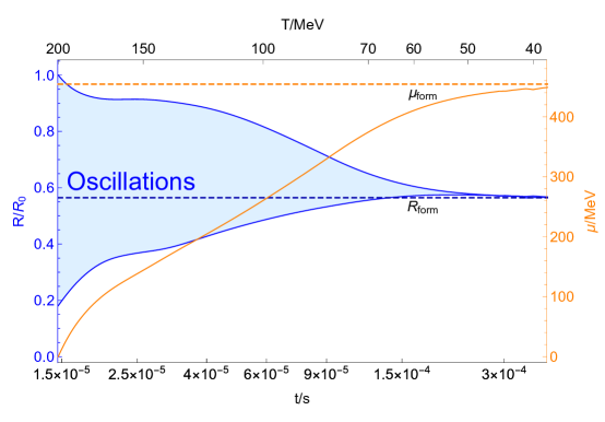
Figure 1: Numerical result of the nugget evolution, adopted from [7], see items 1-3 in the text with explanations of the notations.

The numerical simulations suggest [23] that approximately $87\%$ of the total wall area belong to the percolated large cluster, while the rest $13\%$ is represented by relatively small closed bubbles of different topology. This implies that a finite portion of order $0.1$ of the $N_{\rm DW}=1$ walls are formed as closed surfaces. The collapse of the closed $N_{\rm DW}=1$ bubbles will be halted due to the Fermi pressure acted by the accumulated fermions. As a result, the closed $N_{\rm DW}=1$ bubbles will eventually become the stable AQNs and serve as the dark matter candidates. The corresponding evolution is rather complex as it includes three drastically different scales: the $\Lambda_{\rm QCD}$, the axion mass scale $m_{a}$, and finally the cosmological time evolution scale $t\sim 10^{-4}$ s when the AQN formation occurs. The key elements of this complicated evolution can be summarized as follows:

1. the nugget oscillates numerous number of times with frequency $\omega\sim R^{-1}$ by slowly approaching its final size $R_{\rm form}$, see shaded blue region on Fig. 1;

2. the nugget assumes its final configuration with size $R_{\rm form}$ at $T_{\rm form}\approx 40~{}{\rm MeV}$, see dashed blue line on Fig. 1. This magnitude for $T_{\rm form}$ is consistent with observed value for $\eta$ defined by (2);

3. the chemical potential inside the nugget assumes a sufficiently large value $\mu_{\rm form}\gtrsim 450$ MeV during this long evolution, see orange line on Fig. 1. This magnitude is consistent with formation of a CS phase. Therefore, the original assumption on CS phase which was used in construction of the nugget is justified a posteriori.

We conclude this section with the following comments regarding the formation and survival pattern of the AQNs. First of all, a complete formation of the nugget occurs on a time scale $10^{-4}{\rm s}$ which is precisely the cosmological scale when the temperature drops to $40~{}{\rm MeV}$, see Fig. 1. This scale is known from completely different arguments [24] related to the estimate of the baryon to photon ratio (2). It is a highly nontrivial observation that all these drastically different scales as mentioned above, nevertheless lead to a consistent picture. Secondly, the newly formed nuggets survive an unfriendly environment of a very hot and dense cosmic plasma before and after BBN epoch at $T\sim 0.1\rm~{}MeV$. Furthermore, a long-standing primordial lithium puzzle may find its resolution within the AQN framework as argued in [8]. Third, the dominant portion of the nuggets survive the dramatic events (such as galaxy and star formation) during the long post-recombination evolution of the Universe as argued in [7].

The space limitation here does not allow to cover all these interesting topics in the present review. Instead, we quote the known observational constraints on such kind of objects. Any direct or indirect detection experiments is sensitive to the average value $\langle B\rangle$ for the distribution of the AQNs as any observable consequences will be scaled by the matter-AQN interaction rate along a given line of sight,

$$R^{2}\int d\Omega dl[n_{\rm visible}(l)\cdot n_{\rm DM}(l)]\sim\frac{1}{\langle B\rangle^{1/3}},$$ (3)

where $R\sim B^{1/3}$ and $n_{DM}\sim B^{-1}$ such that effective interaction is suppressed as $B^{-1/3}$ for large nuggets, which represents very generic feature of the model as discussed at the very end of Section 1. Thus, any astrophysical constraints impose a lower bound on the value of $\langle B\rangle$. The relevant constraints come from a variety of both direct detection and astrophysical observations.

The strongest direct detection limit is set by the IceCube Observatory’s non-detection of a nugget flux which can be expressed as

$$\langle B\rangle>3\cdot 10^{24}~{}~{}~{}~{}~{}({\rm direct~{}detection~{}constraint)},$$ (4)

see Appendix A in [25]. Similar limits are also derivable from the Antarctic Impulsive Transient Antenna (ANITA) [26] though this result depends on the details of radio band emissivity of the AQN. There is also a limit [26] from potential contribution to earth’s energy budget which require $|B|>2.6\times 10^{24}$, which is consistent with (4).

3 The AQN model: application to the “solar corona mystery”

In this section we review several recent papers [28, 29, 30, 31] devoted to a possible resolution of the long standing problem, the so-called “solar corona mystery”. We start in subsection 3.1 by reviewing the puzzling observations from corona, while in subsection 3.2 we explain how these mysterious features could be naturally explained within the AQN framework. Finally, in subsection 3.3 we interpret the recently observed radio impulsive events in quiet solar corona as inevitable consequence of the AQN annihilation events.

3.1 The nanoflares: the observations and modelling

We start by explaining the puzzling features of the solar corona which is a very peculiar environment. Indeed, at an altitude of 2000 km above of the photosphere, the plasma temperature exceeds a few $10^{6}$ K. The total energy radiated away by the corona is of the order of $L_{\rm corona}\sim 10^{27}{\rm erg~{}s^{-1}}$, which is about $(10^{-6}-10^{-7})$ of the total energy radiated by the Sun. Most of this energy is radiated at the extreme ultraviolet (EUV) and soft X-ray wavelengths. There is a very sharp (relatively thin, 200 km at most) transition region (TR) where the temperature suddenly jumps from $6\cdot 10^{3}$ K to $10^{6}$ K. This jumps is very uniform and occurs everywhere even in the quiet Sun, where the magnetic field is small, ($\sim 1~{}{\rm G}$), away from active spots and coronal holes. It is very hard to imagine how the temperature increases by factor $10^{2}$ or so over entire surface when the density decreases. These dramatic changes occur on a relatively short length scale $\sim 10^{2}$ km, while a typical scale in the Sun of order $\sim 10^{5}$ km.

A possible solution to the heating problem in the quiet Sun corona was proposed in 1983 by Parker [32], who postulated that a continuous and uniform sequence of miniature flares, which he called “nanoflares”, could happen in the corona. The term “nanoflare” has been used in a series of papers by Benz and coauthors [33, 34, 35, 36], and many others[37, 38, 39, 40] to advocate the idea that these small “nano-events” might be responsible for the heating of the quiet solar corona. Originally, the nanoflares thought to be a “nano”- version of large solar flares when the energy is assumed to be generated by the magnetic field reconnection. However, it is very hard to imagine how the magnetic reconnection could occur in the quiet Sun, where the magnetic field pressure $\sim{\cal{B}}^{2}$ is four orders of magnitude smaller than conventional kinetic pressure $p$. Therefore, more recently, the nanoflares are modelled as invisible (below the instrumental threshold) generic events, producing an impulsive energy release at a small scale without specifying their cause and their nature, see reviews [39, 40]. The list of puzzling features includes:

1. The EUV emission is highly isotropic [35, 36], in huge contrast with flares which are much more energetic and occur exclusively in active areas. Therefore the nanoflares have to be distributed very uniformly everywhere, including large areas of quiet regions;

2. According to [34], in order to reproduce the measured EUV excess, the observed range of nanoflares needs to be extrapolated from the observed events interpolating between $(3.1\cdot 10^{24}-1.3\cdot 10^{26})~{}{\rm erg}$ to unresolved events with energies $10^{22}$ erg and even lower;

3. Time measurements of many nanoflares demonstrate the Doppler shift with a typical velocities (250-310) km/s, far exceeds the thermal ion velocity which is around 11 km/s [33];

4. The EUV emission from the corona shows a modest variation during the solar cycles, not exceeding factor (3-4). It should be contrasted with enormous fluctuations $\sim 10^{2}$ of the large flare’s frequency of appearance during the same cycles, see Fig. 1 from[41].

If the magnetic reconnection were fully responsible for both the large flares and nanoflares, then the variation during the solar cycles should be similar for these two phenomena. It is not what is observed: the variation of the EUV during the solar cycles is relatively modest and does not normally exceed factor of 3 or so, while the variation of the flare’s activity during the same solar cycles very often exceeds factor $10^{2}$. Therefore, the source of the uniform and persistent EUV radiation must be very different from the magnetic field activity responsible for the large flares. In particular, the EUV emission from corona never stops even when the large flare activity is not observed for months. The source of this persistent EUV radiation still remains a big mystery.

3.2 The nanoflares as the AQN annihilation events

In this subsection we explain how these observed puzzling features listed above are naturally occur in the AQN framework. It has been conjectured in [28] that the nanoflares can be identified with the AQN annihilation events when the nuggets hit the sun and release their entire energy to corona. From this identification it follows that the total AQN’s annihilating charge should equal to the energy of a nanoflare. Furthermore, the baryon charge distribution within AQN framework and the nanoflare energy distribution must be one and the same function [28], i.e.

$$dN\propto B^{-\alpha}dB\propto W^{-\alpha}dW\iff[\rm nanoflares\equiv AQN~{}annihilation~{}events],$$ (5)

where $dN$ is the number of nanoflare events with energy between $W$ and $W+dW$, which occur as a result of complete annihilation of the antimatter AQN carrying the baryon charges between $B$ and $B+dB$.

An immediate self-consistency check of this conjecture is the observation that the allowed constraint (4) for the AQNs baryonic charge $B$ is consistent with the nanoflare energy $W$ as these two values become connected as $W\approx 2~{}{\rm GeV}\cdot B$. In particular, the minimal baryon charge $B_{\rm min}\simeq 3\cdot 10^{24}$ from (4) corresponds to the released energy by a nanoflare $W_{\rm min}\simeq(2~{}{\rm GeV})B_{\rm min}\simeq 10^{22}$ erg, which is a proper scale for the extrapolation to the unresolved events as mentioned in item 2 from previous subsection 3.1. One should emphasize that this is a highly nontrivial self-consistency check of the proposal [28] as the acceptable range for the AQNs and nanoflares have been constrained from drastically different physical systems.

We are now in position to present several additional arguments to support this proposal: item 1 from previous subsection 3.1 is also naturally explained in the AQN framework as the DM is expected to be distributed very uniformly over the Sun making no distinction between quiet and active regions, in contrast with large flares. A similar argument applies to item 4 as the strength of the magnetic field and its localization is absolutely irrelevant for the nanoflare events in form of the AQNs, in contrast with conventional paradigm when the nanoflares are thought to be simply scaled down configurations of their larger cousin which are much more energetic and occur exclusively in active areas and cannot be uniformly distributed. It is also consistent with observation that the temporal modulation of the EUV irradiance over a solar cycle is very small and does not exceed a factor $\sim 3$, as opposed to the much dramatic changes in Solar activity with modulations on the level of $10^{2}$ over the same time scale. This suggests that the energy injection from the nanoflares is weakly related to the Solar activity.

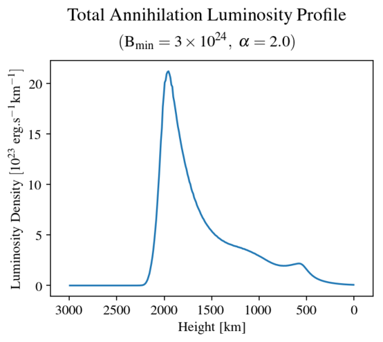
Figure 2: Total EUV luminosity as a function of height, adopted from [30]. It is a highly nontrivial consequence of the conjecture (5) that the most of the energy is released in the narrow TR around 2000 km, where it is known that the most of the drastic changes occur.

The presence of the large Doppler shift with a typical velocities (250-310) km/s, mentioned in item 3, can be understood within the AQN framework as follows: the typical velocities of the nuggets entering the solar corona is very high, around 700 km/s. The Mach number $M=v_{\rm AQN}/c_{s}$ is also very large. A shock wave will be inevitably formed and will push the surrounding material to the velocities which are much higher than would normally present in the thermal equilibrium with its velocity on the level $11\rm km/s$.

Encouraged by these self-consistency checks the authors of [30] literally used the distribution function $f(W)$ which was previously used in [37, 38] to fit the solar data. This step represents a precise realization of the identification (5) with power-law index $\alpha$ which normally lies in the window $\alpha\in(2-2.5)$ to fit the corona observations. This identification allows to describe the AQN’s baryon number distribution $dN/dB$. It can be used for the solar corona as well as for any other applications.

$$\frac{dN}{dB}\propto f(B)\propto B^{-\alpha},~{}~{}~{}~{}\langle B\rangle=\int_{B_{\rm min}}^{B_{\rm max}}dB~{}[B~{}f(B)],~{}~{}~{}\int_{B_{\rm min}}^{B_{\rm max}}dB~{}f(B)=1,$$ (6)

where $B_{\rm min}$ and $B_{\rm max}$ were also fixed using the identification (5).

With explicit models for the distribution function $f(W)$ and with absolute normalization for the AQN’s flux determined by the DM density $\rho_{\rm DM}\approx 0.3~{}\rm GeV/cm^{3}$ one can proceed with Monte Carlo (MC) simulations to study a number of interesting questions related to the dynamics of the AQNs when they propagate in solar atmosphere. The results of the corresponding studies performed in [30] were remarkable: the total energy rate injection into the solar corona as a result of the AQN annihilation processes is very close to the observed value $L_{\rm corona}\sim 10^{27}{\rm erg~{}s^{-1}}$. Furthermore, this energy is mostly deposited in the TR around 2000 km as mentioned in Section 3.1, see Fig.2. It could explain the nature of this region when very sharp changes in temperature occur on a very small scale as a result of the AQN annihilation processes in this transition region.

3.3 Impulsive radio events in quiet solar corona

As discussed in the previous subsections the individual short energy bursts associated with these nanoflares are below detection limits and have not yet been directly observed in the EUV or X-ray regimes. In fact, all coronal heating models advocated so far, including [37, 38] require the existence of an unobserved (i.e. unresolved with current instrumentation) source of energy distributed over the entire Sun. However, it has been recently claimed in [42] that radio observations can potentially “see” individual nanoflares and their “internal structures”, where more energetic EUV and X-rays instruments cannot, while the intensity at the radio frequencies is many orders of magnitude smaller than more energetic EUV and X-rays radiation.

In our recent paper [31] it has been argued that the radio emission fits in the AQN annihilation events. It has been also argued that the impulsive radio events in the quiet solar corona as recorded by the Murchison Widefield Array (MWA) [42] match well the computations based on the AQN framework. This claim has been supported by demonstrating that the generic features of the observations in the radio frequency bands such as the rate of appearance, the temporal and spatial distributions and their energetics represent the natural consequences of the AQN annihilation events in the quiet corona.

The basic idea of the radio emission due to the AQN annihilation events can be briefly explained as follows. It is generally accepted that the radio emission from the corona results from the interaction of plasma oscillations (also known as Langmuir waves) with non-thermal electrons which must be injected into the plasma by some non-thermal mechanism[43]. The plasma instability develops when the injected electrons have a non-thermal high energy component at which point the radio waves can be emitted. The frequency of emission $\nu$ is mostly determined by the plasma frequency $\omega_{p}$ in a given environment, i.e.

$$\omega^{2}=\omega_{p}^{2}+k^{2}\frac{3T}{m_{e}},~{}~{}~{}\omega_{p}^{2}=\frac{4\pi\alpha n_{e}}{m_{e}},~{}~{}~{}\nu=\frac{\omega}{2\pi},$$ (7)

where $n_{e}$ is the electron number density in the corona at altitude $h$, while $T$ is the temperature at the same altitude and $k$ is the wavenumber. The emission of radio waves generically occurs at high altitudes $h\sim 10^{4}$ km where the energy is injected into the plasma. The non-thermal electrons received their kinetic energy at much lower altitude $h\simeq 2000$ km where the AQNs release their annihilation energy as discussed in previous subsection, see Fig.2. After that they can propagate upward for very long distance determined by the mean free path $\lambda\sim 10^{4}$ km before they transfer their energy to the radio waves. It is known that the number density of the non-thermal (supra-thermal in terminology [43]) electrons $n_{s}$ must be sufficiently large $n_{s}/n_{e}\gtrsim 10^{-7}$ for the plasma instability to develop, in which case the radio waves will be generated [43]. As the density $n_{s}/n_{e}$ approaches the threshold values at some specific frequencies, the intensity increases sharply, which we identify with the observed impulsive radio events. These threshold conditions may be satisfied randomly in space and time, depending on properties of the injected electrons and properties of the surrounding plasma[43].

It has been demonstrated in [31] that the number density of the non-thermal electrons $n_{s}$ generated by the AQNs can easily assume a proper range $n_{s}/n_{e}\gtrsim 10^{-7}$ for the plasma instability to develop when these non-thermal electrons reach the altitudes $h\sim 10^{4}$ km where the radio emission occurs as the plasma frequency $\omega_{p}(h)$ assumes a proper value (7). It has been also shown that the frequency of the impulsive events, their temporal and spatial distributions are consistent with results recorded by the MWA [42]. Furthermore, it has been also shown that the non- Poissonian feature as shown on Fig 7 of [42] is also naturally explained in the AQN framework. Indeed, the AQN annihilation events always will be accompanied by the clustering of radio events as the non-thermal electrons from one and the same AQN may release their energy at different altitudes and different instants which lead to the clustering events as observed.

We conclude this section with the following comments. A close similarity between the observed value for the EUV luminosity $\sim 10^{27}{\rm erg~{}s^{-1}}$ and computed value within the AQN framework is a highly nontrivial consequence of the proposal [28] as the general normalization in the AQN based computation is determined by the DM density $\rho_{\rm DM}\approx 0.3~{}\rm GeV/cm^{3}$ rather than by internal physics of the Sun. The emergence of a small scale $\sim 200$ km which determines the TR is also entirely determined by the internal structure of the nuggets, their internal temperature and ionization properties. Precisely these features determine very fast increase of the annihilation rate at the altitude around 2000 km as shown on Fig.2. Both these consequences of the AQN proposal can be considered as “miracle coincidences” as there are no any free parameters in the corresponding estimates, see also footnote 7 with a relevant comment.

One may wonder if the AQNs play any role in dynamics of the large solar flares which are characterized by dramatically different energy scales (in comparison with nanoflares) with $W\simeq(10^{26}-10^{32})~{}\rm erg$. It has been proposed in [29] that the AQNs hitting the active regions with large magnetic field may play the role of the triggers which could ignite and initiate the magnetic reconnections leading to large solar flares. There is no room to elaborate on this interesting relation, and we refer to the original paper [29] for the details.

The direct observation of the individual nanoflares which represent the AQN annihilation events according to the conjecture (5) is hard to test directly in the EUV or X-ray regimes as the current instruments do not have sufficient resolution.

At present time we think the most promising tests of this proposal can be achieved in the radio frequency bands. In particular, there must be spatial and temporal correlations between radio events in a given local region, in the different frequency bands, with time delays measured in seconds. Similar clustering events in the same frequency band have been observed by MWA [42]. We advocate the idea that similar spatial and temporal correlations must also exist in different frequency bands. This prediction can be directly tested and analyzed by MWA since, according to [42], the data in the 179, 196, 217 and 240 MHz bands have been recorded, but not published yet.

Another generic consequence of this framework is that the lower frequencies waves being emitted from higher altitudes must be suppressed while the intensity of the higher frequency bands must be enhanced. This is because the upward moving non-thermal electrons are much more numerous at lower altitude (corresponding to higher $\nu$) in comparison to higher altitudes (corresponding to lower $\nu$). This prediction can be also directly tested in future studies. Finally, the Solar Orbiter recently observed so-called “campfires” in the extreme UV frequency bands. It is tempting to identify such events with the annihilation of large sized AQN (which are rare events), as they are capable of generating radio signals sufficiently strong to be resolved. We therefore suggest to search for a cross correlation between MWA radio signals and recordings of the extreme UV photons by Solar Orbiter.

4 The AQN model: application to observed “Mysterious Bursts”

In this section we review two recent papers [44, 45] devoted to explanation of the observed by the Telescope Array (TA) puzzling events, the so-called bursts[46, 47]. These events are very unusual and cannot be interpreted in terms of conventional single showers as reviewed below. These events have been coined in [44] as the “Mysterious Bursts”.

We start in subsection 4.1 by reviewing the unusual and very distinct features of the TA-bursts [46, 47], while in subsections 4.2 and 4.3 we explain how these puzzling features could be accommodated within the AQN framework[44]. Finally, in subsection 4.4 we argue that TA bursts will be inevitably accompanied by the radio signals in frequency band $\nu\in(0.5-200)$ MHz. These radio signals must be synchronized with the TA bursts. The observation of such unique synchronization can unambiguously support, substantiate or refute this proposal.

4.1 The TA-bursts: observations

The unusual features of the bursts recorded by [46, 47] can be briefly formulated as follows:

1. “curvature puzzle”. All reconstructed air shower fronts for the burst events are much more curved than usual cosmic ray (CR) air showers. This feature is expressed in terms of the time- spreading versus spatial-spreading of the particles in the bursts. The corresponding “curvature” is much more pronounced for the bursts in comparison with conventional CR air showers, see see Fig. 3 and Fig. 4 in [46]. Furthermore, the bursts events do not have sharp edges in waveforms in comparison with conventional CR events;

2. “clustering puzzle”. The events are temporally clustered within 1 ms, which would be a highly unlikely occurrence for three consecutive conventional high energy CR hits in the same area within a radius of approximately 1 km. The total 10 burst events have been observed during 5 years of observations. The estimated energy from individual events within the bursts is five to six orders of magnitude higher than the energy estimated by event rate.

3. “synchronization puzzle”. Most of the observed bursts are “synchronized” (time delay between burst and lightning is less than 1 ms) or “related” (time delay between burst and lightning is less than 200 ms) with the lightning events. Some of the bursts are not related to any lightnings. However, all 10 recorded bursts occur under thunderstorms.

It is very hard to understand all these features in terms of conventional CR physics as the bursts cannot be reconciled with conventional CR physics. At the same time all unusual features (including the energetics, the flux estimates, the time and spatial spreading of each event within the bursts) can be naturally explained within the AQN framework. Before we proceed with corresponding explanation we have to briefly overview the basic features of the AQNs propagating under thunderclouds to explain the nature and the source of the TA bursts.

4.2 The AQNs under the thunderclouds

The AQNs made of antimatter are capable to release a significant amount of energy when they enter the Earth’s atmosphere and annihilation processes start to occur between antimatter hidden in form of the AQNs and the atmospheric material. The emission of positrons from the nuggets made of antimatter during the thunderstorms plays the crucial role in the proposal [44]. The liberation of the positrons from the AQNs occurs because the thunderclouds are characterized by large preexisting electric field $\cal{E}$. This field liberates and accelerates the positrons which are normally bound to the AQNs with a typical average binding energy of order $\rm keV$.

The presence of the electric field $\cal{E}$ under thunderclouds is well established phenomenon. It is characterized by the following parameters [48, 49]:

$${\cal{E}}\simeq{\rm\frac{kV}{cm}},~{}~{}~{}~{}l_{a}\simeq 100~{}{\rm m},~{}~{}~{}~{}\tau_{\cal{E}}\simeq\frac{l_{a}}{c}\simeq 0.3{\rm\,\mu s},$$ (8)

where $l_{a}$ is the so-called avalanche length. If the AQN enters the electric field (8) along its path it may liberate the positrons from the AQN’s electrosphere as the additional energy $\Delta E$ assumes the same order of magnitude as the binding energy $E_{\rm bound}\sim\rm keV$ of the positrons, i.e.

$$\Delta E\simeq[e{\cal{E}}\cdot R_{\rm cap}]\sim 2\rm~{}keV\gtrsim E_{\rm bound},$$ (9)

where parameter $R_{\rm cap}$ is a typical distance where positrons reside, and can be estimated in terms of the ionization charge $Q$ and internal temperature of the nuggets $T\simeq 10\rm~{}keV$ as follows:

$$R_{\rm cap}\simeq\frac{\alpha Q}{T}\sim 2~{}{\rm cm},$$ (10)

see [44] with proper estimates. This additional energy (9) of order of several keV could liberate the positrons from the nuggets, which consequently will be accelerated to MeV energies on $l_{a}$ length scale. Indeed,

$$E_{\rm exit}\simeq[e{\cal{E}}\cdot l_{a}]\sim 10\rm~{}MeV.$$ (11)

This estimate suggests that the positrons assume $10\rm~{}MeV$ energy after they exit the region of strong electric field which is known to exist under thunderclouds. It is very important to emphasize that these estimates hold because the initial energy of the positrons is relatively high, in keV scale according to (9) such that they do not immediately annihilate, which would be the case for the positrons with eV energies. Due to the same reasons the positrons do not experience strong elastic scattering and remain in the electric field background (8) during entire period of acceleration which lasts about $0.3{\rm\,\mu s}$, see also a footnote 8 with related comment.

4.3 “Mysterious bursts” as the AQN annihilation events

The goal of this subsection is to explain how the unusual features listed in subsection 4.1 can be naturally understood within the AQN framework.

4.3.1 “curvature puzzle”

In the AQN proposal[44] the “curved” feature can be easily understood by noticing that essential parameter in this proposal is the initial spread of the particles determined by angle $\Delta\alpha\simeq\left({v_{\perp}}/{c}\right)\in(0-0.1)$. This spread in $\Delta\alpha$ is determined by the velocity distribution perpendicular to electric field at the exit point. The corresponding distribution can be expressed in terms of the initial energy (9) as follows $v_{\perp}\simeq\sqrt{2\Delta E/m}\lesssim 0.1c$. Therefore, after travelling the distance $r$ the spatially spread range $\Delta s$ is estimated as

$$\Delta s\simeq r\left(\frac{\Delta\alpha}{\cos\alpha}\right)\simeq\frac{1~{}{\rm km}}{\cos\alpha}\left(\frac{r}{10\rm~{}km}\right)\left(\frac{\Delta\alpha}{0.1}\right),$$ (12)

see Fig. 3 for precise definitions of the parameters. At the same time, the temporal spread $\Delta t$ can be estimated as follows:

$$\Delta t\simeq\frac{\Delta r}{c}\simeq 3{\rm\,\mu s}\cdot(\tan\alpha)\cdot\left(\frac{r}{10\rm~{}km}\right)\left(\frac{\Delta\alpha}{0.1}\right)$$ (13)

where $\Delta r\simeq r\tan\alpha\Delta\alpha$, see Fig. 3. These parameters are linearly proportional to each other and assume proper values consistent with observations. Indeed,

$$c\Delta t\simeq\Delta s\sin\alpha,~{}~{}~{}\Delta\alpha\simeq\left(\frac{v_{\perp}}{c}\right)\in(0-0.1)$$ (14)

such that $2\Delta t$ may vary between $(0.5-8){\rm\,\mu s}$ when $2\Delta s$ changes between $(0.5-2)$ km with approximately linear slope determined by electric field direction $\sin\alpha$ which is consistent with observed events presented on Fig. 3 and Fig. 4 in [46]. We use $(2\Delta t)$ and $2\Delta s$ in our estimates with extra factor 2 as the angle $\Delta\alpha=(v_{\perp}/c)$ could assume the positive or negative value, depending on sign of $v_{\perp}$ with respect to instant direction of the electric field $\mathbf{{\cal{E}}}$ as shown on Fig. 3.

This behaviour in terms of the temporal and spatial spreads for the bursts should be contrasted with conventional CR distribution when the timing spread is much shorter and always below $2{\rm\,\mu s}$ while the spatial spread is much longer, up to 3.5 km, see Fig. 5 in [46]. This difference between the distributions in bursts and conventional CR air showers was coined as the “curvature” puzzle, which is naturally resolved within the AQN framework as argued above.

Similar arguments also explain why the observed events do not demonstrate any sharp edges in waveforms (see Fig. 6 in [46]). This is because the conventional CR air showers typically have a single ultra-relativistic particle generating a very sharp edge in waveforms. It should be contrasted with large number of positrons which produce the non-sharp edges in waveforms in the AQN-based proposal.

Figure 3: The geometry of the TA bursts, adopted from [44]. The angular spread of the propagating positrons is determined by $\Delta\alpha\ll\alpha$. The spatial spread on the surface is determined by $\Delta s$, while the temporal spread is determined by $\Delta r/c$. The altitude is assumed to be within conventional range $h\simeq(4-12)$ km. Instant direction of the electric field $\mathbf{\cal{E}}$ at the moment of exit of the positrons is also shown.

4.3.2 “clustering puzzle”

The “clustering puzzle” represents a dramatic inconsistency for the burst events if one assumes the randomness of the events described by conventional Poissonian distribution. The event rate suggests that the energy should be in $10^{13}$ eV range, while the intensity of the events suggests $(10^{18}-10^{19})$ eV range, if one interpret the events as conventional CR air showers. It should be contrasted with the AQN framework when the bursts represent the cluster of events (not a collection of independent random events). The conventional Poissonian distribution does not apply here. The presence of several events within the same burst is a natural consequence of the AQN’s slow velocity when it merely propagates $\sim 0.25$ km during 1 ms and it always remains in the same thunderstorm system characterized by the fluctuating electric field $\cal{E}$. The spatial spread for each individual event within the same cluster also lies within the range (12), being consistent with observations.

4.3.3 “synchronization puzzle”

Most of the observed bursts are “synchronized” or “related” to the lightning events. Few events are not related to the lightnings, but all 10 recorded bursts occurred under thunderstorms. This is very puzzling property of the bursts if interpreted in terms of the conventional CR air showers because it is very hard to understand how the thunderstorms may dramatically modify CR features as discussed above.

At the same time the “synchronization” puzzle is perfectly consistent with AQN based proposal [44] because the thunderstorm with its pre-existing electric field (8) plays a crucial role in the mechanism as the electric field is always present under the thunderclouds irrespectively to the lightning flashes. This strong electric field instantaneously liberates the positrons and also accelerates them up to 10 MeV energies. These positrons can easily reach the TA surface detectors, and can produce the signals consistent with the bursts.

4.4 Radio signal from “Mysterious bursts”

In this subsection we highlight the basic ideas of the recent studies [45] devoted to analysis of the radio signals which always accompany TA bursts when interpreted in terms of the AQN annihilation events under the thunderstorm as presented in previous section 4.3. We shall argue below that the radio emission is inevitable consequence of the proposed explanation of the TA bursts when the positrons are accelerating in external electric field $\cal{E}$ under thunderclouds with typical duration $\tau_{\cal{E}}\simeq 0.3{\rm\,\mu s}$ as reviewed in subsection 4.2.

The starting point for these studies is spectral property of the electric field $\mathbf{E}_{\omega}$ at distance $R$, which is generated by accelerating positrons:

$$\mathbf{E}_{\omega}=\int_{-\infty}^{+\infty}\mathbf{E}e^{i\omega t}dt=\frac{e^{ikR}}{R}\left(\frac{Ne}{c^{2}}\right)\left(\frac{\omega}{\omega^{\prime}}\right)^{2}\left[\mathbf{n}\times\left((\mathbf{n}-\frac{\mathbf{v}}{c})\times\mathbf{a}_{\omega^{\prime}}\right)\right],~{}~{}~{}$$ (15)

where all quantities at the right hand side of (15) must be computed at the retarded times $t^{\prime}\approx t-\frac{R}{c}+\frac{\mathbf{n}\cdot\mathbf{v}t^{\prime}}{c}$. The coefficient $N$ in formula (15) is the number of the coherent positrons participating in the emission, while parameters $\omega^{\prime}$ and $\mathbf{a}_{\omega^{\prime}}$ entering (15) are defined as follows:

$$\omega^{\prime}\equiv\omega\left(1-\frac{\mathbf{n}\cdot\mathbf{v}}{c}\right)\approx\frac{\omega}{2}\left[\frac{1}{\gamma^{2}}+{\theta^{2}}\right],~{}~{}\mathbf{a}_{\omega^{\prime}}=\int_{-\infty}^{+\infty}\mathbf{a(t^{\prime})}e^{i\omega^{\prime}t^{\prime}}dt^{\prime},~{}~{}\mathbf{a}(t)\approx\frac{e{{\cal{E}}(t)}}{\gamma^{3}m}.~{}~{}~{}$$ (16)

The spectral density of the emission $dE_{\omega}/d\omega$ can be computed in terms of these variables as follows:

$$\frac{dE_{\omega}}{d\omega} = \left(\frac{N^{2}e^{2}\gamma^{6}}{2\pi c^{3}}\right)\frac{16|\mathbf{a}_{\omega^{\prime}}|^{2}}{(1+\gamma^{2}\theta^{2})^{3}}\left[\frac{\gamma^{2}\theta^{2}}{1+\gamma^{2}\theta^{2}}\right]\frac{d\Omega}{2\pi},~{}~{}~{}~{}\gamma\equiv\frac{1}{\sqrt{(1-\frac{v^{2}}{c^{2}})}},$$ (17)

where $|\mathbf{a}_{\omega^{\prime}}|$ should be expressed in terms of $\theta$ according to (16). Significance of this formula is that it explicitly shows that the emission mostly occurs along the small angles $\theta\simeq\gamma^{-1}$, as expected. Another important feature of the spectral density $dE_{\omega}/d\omega$ is that the radio pulse occurs in bandwidth $\nu\in(0.5-200)\rm~{}MHz$ and lasts for about $\tau_{\cal{E}}\simeq 0.3{\rm\,\mu s}$, see [45] for the details.

The next task is to estimate the intensity of the electric field (15) at very large distances $R$ where it can be potentially detected. The orientation of $\mathbf{E}$ field is determined by cross product (15) where one can assume (for the simplicity of the numerical estimates) that $\mathbf{v}\parallel\mathbf{a}$. The absolute value for $|\mathbf{E}|$ at large distances can be estimated as follows

$$|\mathbf{E}|\approx\frac{Ne|\mathbf{a}|\theta}{c^{2}R}\left(\frac{2\gamma^{2}}{1+\gamma^{2}\theta^{2}}\right)^{3}\approx 90{\rm\frac{mV}{m}}\left[\frac{(\gamma\theta)}{(1+\gamma^{2}\theta^{2})^{3}}\right]\left(\frac{\gamma}{20}\right)^{2}\left(\frac{N}{10^{9}}\right)\left(\frac{\rm 10~{}km}{R}\right).~{}~{}$$ (18)

The distance $R$ in this equation should not be confused with parameter $r$ which enters all formulae from previous subsection 4.3, including Fig. 3.

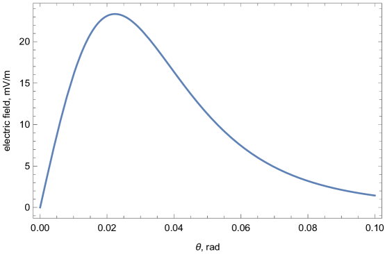
Figure 4: Strength of the AQN-induced electric field (18) versus observation angle $\theta$, adopted from [45]. The parameters are chosen to be $N=10^{9}$, $\gamma=20$. The electric field under thunderclouds is chosen to be ${\cal E}=1{\rm\,kV/cm}$ consistent with (8).

The expression (18) has been derived under assumption that the acceleration $|\mathbf{a}|$ is a constant during time $t\in(0,\tau_{{\cal{E}}})$. The dependence of $|\mathbf{E}(\theta,t)|$ as a function of the $\theta$ is shown on Fig. 4 for typical parameters of the system. The key unknown parameter $N$ which enters (18) and which essentially determines the absolute value of the $|\mathbf{E}(\theta,t)|$ field was estimated from the assumption that the AQN induced positrons are responsible for puzzling TA burst events with number of particles as recorded by [46]. Therefore, the estimate (18) is self-consistent with our treatment of the TA bursts as the AQN annihilation events under the thunderstorm, as reviewed in subsection 4.3.

One should emphasize that the correlation between lightning and radio emission during thunderstorms is well known and well documented generic feature of the lightning discharges. However, the AQN-induced radio pulses are qualitatively distinct from conventional lightning-induced radio signals. In particular, the lightning-induced radio emission is strongly peaked in few MHz bands, while AQN-induced radio pulse is characterized by the flat spectrum with $\nu\lesssim 200\rm~{}MHz$ according to [45]. Furthermore, the AQN-induced radio pulses must occur before the lightning flash or at the very initial moment of the lightning flashes as the observed bursts demonstrate this feature [46]. It should be contrasted with the lightning-induced radio signals which occur during the late stages of the lightning discharges. Based on these dramatic differences in frequencies and timings of the radio emissions one safely concludes that the signals due to the thunderstorm lightning events can be easily discriminated from the AQN-induced radio pulses.

To summarize this section: the mysterious bursts (with highly unusual features as reviewed in sections 4.1) are naturally interpreted as the cluster events generated by the AQN annihilation events under thunderstorm as reviewed in 4.3. Some features of the system such as given by (12), (13), (14) are not sensitive to many uncertainties related to complex dynamics of the AQN propagating under the thunderclouds. These features represent almost model-independent consequences of the proposal [44] because they are based exclusively on geometrical and kinematical features of the system. Furthermore, the radio pulse (18) which is inevitable consequence of the proposal must be synchronized within $10{\rm\,\mu s}$ with TA burst irrespectively whether the bursts are related or unrelated to the lightning events because the positrons and radio waves emitted from the same location at the same instant and both propagate with the speed of light. Therefore, observing (not observing) such synchronized signals can confirm, substantiate or refute this proposal.

5 The axions from AQNs: broadband axion searches

As we explained in sections 1 and 2 the axion field is at heart of the AQN construction as it plays a dual role: it makes the nuggets absolutely stable configurations as a result of extra pressure due to the axion domain walls surrounding the quark matter. The same $\cal{CP}$ odd axion field plays a vital role for baryon charge segregation, replacing the conventional baryogenesis. However, the corresponding axion energy (hidden in the form of the axion domain wall) is not available unless the AQN’s baryon charges from the nugget’s core start annihilating processes with surrounding material. This axion domain wall field which (in empty space) equilibrates the Fermi pressure of the quark matter will start to adjust to these changes, and the axion energy will be released into the space in the form of the free propagating axions which can be observed by the axion detectors. The goal of the present section is to highlight the basic ideas developed in [50, 51, 52, 53, 54] on possible strategy to search for such AQN-induced axions.

In next subsection 5.1 we explain the dramatic difference between the galactic axions and the axions which are produced as a result of the annihilating processes when the AQN enters the atmosphere and crosses the Earth. The resulting spectrum of the axions will be drastically different from conventional galactic non-relativistic axions with $v_{\rm axion}\sim 10^{-3}c$. This difference in spectrum dictates a new broadband strategy to search the AQN-induced axions which is the topic of the subsection 5.2

5.1 Spectral features of the AQN-induced axions

For the purposes of the present work it is sufficient to mention that the conventional dark matter galactic axions are produced due to the misalignment mechanism when the cosmological field $\theta(t)$ oscillates and emits cold axions before it settles down at its final destination $\theta_{\rm final}=0$, see recent reviews [19, 21, 22]. Another mechanism is due to the decay of the topological objects. It is important that in both cases the produced axions are non-relativistic particles with typical $v_{\rm axion}/c\sim 10^{-3}$, and their contribution to the dark matter density scales as $\Omega_{\rm axion}\sim m_{a}^{-7/6}$. This scaling unambiguously implies that the axion mass must be fine-tuned $m_{a}\lesssim 10^{-5}$ eV to saturate the DM density today, while larger axion mass will contribute very little to $\Omega_{\rm DM}$. The cavity type experiments have a potential to discover these non-relativistic axions. Axions can be also produced as a result of the Primakoff effect in a stellar plasma at high temperature see recent reviews [19, 20, 21, 22]. These axions are ultra-relativistic as the typical average energy of the axions emitted by the Sun is $\langle E\rangle=4.2$ keV.

There is a fundamentally novel mechanism of the axion production when the AQNs enter stars or planets[50]. This mechanism is rooted to the AQN dark matter model. The most important feature of the emitted axions is that these emitted axions will be released with relativistic (but not ultra-relativistic) velocities with typical values $v_{\rm axion}^{\rm AQN}\simeq 0.6c$. These features should be contrasted with conventional galactic non-relativistic axions $v_{\rm axion}\sim 10^{-3}c$ and solar ultra-relativistic axions with typical energies $\langle E\rangle=4.2$ keV.

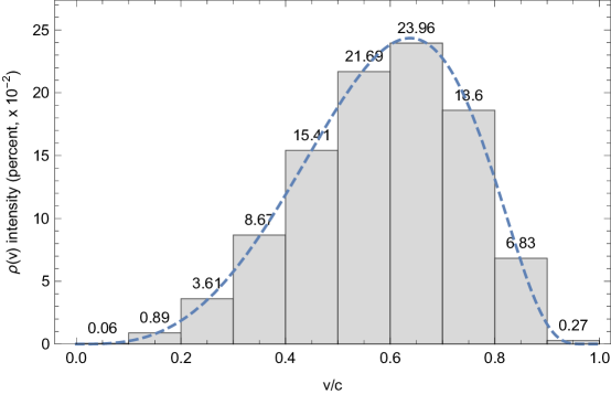
Figure 5: Normalized spectrum $\rho(v)$ of the AQN-induced axions, adopted from [51].

The new mechanism of production of these axions can be explained as follows. The total energy of an AQN finds its equilibrium minimum when the axion domain wall contributes about 1/3 of its total mass [11]. This configuration in the equilibrium does not emit any axions as a result of pure kinematical constraint: the static domain wall axions are off-shell non-propagating axions. However, this static picture drastically changes when some baryon charge from the AQN get annihilated as a result of interaction with environment when the time dependent perturbations obviously change this equilibrium configuration. In other words, the configuration becomes unstable with respect to emission of the axions because the AQN is no longer at its minimum energy configuration with fewer baryon charge in the quark nugget core. As a result of these annihilation processes, the AQN starts to loose its mass, and consequentially its size starts to shrink. To reiterate: the annihilation of antinuggets when an AQN hits the stars or planets forces the surrounding domain wall to oscillate. These oscillations of domain wall generate excitation modes and ultimately lead to radiation of the propagating axions. The spectrum of the corresponding AQN-induced axions has been computed in [51], and we present the corresponding results in Fig. 5.

There are several important features of this spectrum which are deserved to be mentioned here. First of all, typical value $v_{\rm axion}^{\rm AQN}\simeq 0.6c$ is very large in comparison with velocities of conventional galactic non-relativistic axions $v_{\rm axion}\sim 10^{-3}c$. When the AQN hits the Earth and the annihilation processes start the axions will be also emitted as explained above. The corresponding axion density on the Earth’s surface has been computed using full scale Monte Carlo simulations [52]. The results of these computations can be expressed as follows:

$$\langle\rho_{\mathrm{a}}^{\rm AQN}(R_{\oplus})\rangle\sim 5\cdot 10^{-6}{\rm\frac{GeV}{cm^{3}}},~{}~{}~{}\langle v_{\mathrm{a}}^{\rm AQN}(R_{\oplus})\rangle\simeq 0.6c.$$ (19)

These axions are mostly produced in deep Earth’s underground where the density of surrounding material is the highest. One should also note that on average a typical nugget looses approximately $30\%$ of its baryon charge when crosses the Earth. Axion domain wall shrinks correspondingly, which eventually generates the axion density (19). The resulting number density $n_{a}^{\rm AQN}\simeq\rho_{\mathrm{a}}^{\rm AQN}/m_{a}$ is approximately 5 orders of magnitude smaller than conventional galactic axion number density assuming that the galactic non-relativistic axions saturate the DM density observed today. However, the flux $(v_{\mathrm{a}}^{\rm AQN}n_{a}^{\rm AQN})$ related to relativistic axions (19) is only 2 orders of magnitude smaller than conventional flux of non-relativistic axion. Furthermore, due to the greater velocities $v_{\mathrm{a}}^{\rm AQN}$ these axions interact with material in dramatically different way, which could strongly enhance the likelihood of their detection.

One should also mention that these axions can be treated as a classical field because the number of the AQN-induced axions (19) accommodated by a single de-Broglie volume is very large in spite of the fact that the de-Broglie wavelength $\lambda$ for relativistic AQN-induced axions is much shorter than for galactic axions,

$$n_{a}^{\rm AQN}\lambda^{3}\sim\frac{\langle\rho_{\mathrm{a}}^{\rm AQN}(R_{\oplus})\rangle}{m_{a}}\cdot\left(\frac{\hbar}{m_{a}v_{a}}\right)^{3}\sim 10^{6}\left(\frac{10^{-4}{\rm eV}}{m_{a}}\right)^{4}\gg 1.$$

Another comment we would like to make is as follows. The production of the low energy axions with $v_{a}\ll c$ is strongly suppressed as one can see from Fig. 5. However, the axions which are produced with extremely low velocities $v_{a}\lesssim 11\rm~{}{km}/{s}$ will be trapped by the Earth’s gravitational field. These axions will be orbiting the Earth indefinitely, and therefore they will be accumulated around the Earth during entire life time which is 4.5 billion years.

The corresponding Monte Carlo simulations have been performed in [51] with the following estimate:

$$\rho_{\mathrm{a}}(R_{\oplus})\sim 10^{-4}{\rm\frac{GeV}{cm^{3}}},~{}~{}~{}\langle v_{\mathrm{a}}(R_{\oplus})\rangle\simeq 8\rm\frac{km}{s}~{}~{}~{}[\rm gravitationally~{}bound~{}axions].$$ (20)

The number density of the bound axions is at least 2 orders of magnitude smaller than conventional axion number density assuming that the galactic non-relativistic axions saturate the DM density. However, the corresponding wavelength $\lambda_{\mathrm{a}}\sim{\hbar}/({m_{\mathrm{a}}v_{\mathrm{a}}})$ of the gravitationally bound axions is approximately $30$ times greater than for galactic axions, which have a typical velocity of about $\sim 250$ km/s. Therefore, coherent effects can be maintained for a longer period of time in comparison with the case of conventional galactic axion searches. One may hope that this feature of having a large coherence length, $\lambda_{\mathrm{a}}\sim v_{\mathrm{a}}^{-1}$, could play a key role in design of specific instruments, capable of discovering such gravitationally trapped axions.

5.2 Broadband search strategy for the AQN-induced axions

The large average velocities $\langle v_{a}\rangle\simeq 0.6c$ of the emitted axions by AQNs dramatically changes entire strategy of axion searches. This is because the axions are characterized by broad distribution with $m_{a}\lesssim\omega_{a}\lesssim 1.8~{}m_{a}$ as discussed in previous subsection. Therefore, the corresponding axion detectors must be some kind of broadband instruments. For example, if $m_{a}\approx 1$GHz, the detectors must be sensitive at least to the window $(1-2)$ GHz. The cavity type experiments such as ADMX are to date the only ones to probe the parameter space of the conventional QCD axions with $\langle v_{a}\rangle\sim 10^{-3}c$, while we are interested in detection of the relativistic axions with $\langle v_{a}\rangle\sim 0.6c$. This requires a different type of instruments and drastically different search strategies. We assume that some kind of broadband instruments can be designed and built, see reviews [19, 20, 21, 22] with description of possible detectors.

With this assumption in mind, a strategy to probe the QCD axion can be formulated as follows[53]. It has been known since [55] that the DM flux shows annual modulation due to the differences in relative orientations of the DM wind and the direction of the Earth motion around the Sun, which generates the flux difference. The corresponding effect for AQN induced axions was computed in [52]. The daily modulations have been largely ignored in the past because they are numerically very small for WIMP like models. Indeed, the velocity difference due to the Earth’s rotation about its axis is only $\sim$ 0.5 km/s, to be compared with galactic wind $\sim 250$ km/s. The daily modulation in the AQN model is a very specific feature of the AQN model. Full scale Monte Carlo simulations carried out in [52] have shown that the daily modulation could be very large.

The broadband strategy is to separate a large frequency band into a number of smaller frequency bins with the width $\Delta\nu\sim\nu$ according to the axion dispersion relation as discussed above. The time dependent signal in each frequency bin $\Delta\nu_{i}$ has to be fitted according to the expected modulation pattern, daily, or annual. For example, the annual modulation should be fitted according to the following formula

$$A_{\rm(a)}(t)\equiv[1+\kappa_{\rm(a)}\cos\Omega_{a}(t-t_{0})],~{}~{}~{}~{}\rho_{\mathrm{a}}^{\rm AQN}(t)\equiv A_{\rm(a)}(t)\langle\rho_{\mathrm{a}}^{\rm AQN}(R_{\oplus})\rangle$$ (21)

where $\Omega_{a}=2\pi\,\rm yr^{-1}$ is the angular frequency of the annual modulation and label $``a"$ in $\Omega_{a}$ stands for annual. The $\Omega_{a}t_{0}$ is the phase shift corresponding to the maximum on June 1 and minimum on December 1 for the standard galactic DM distribution, see [55, 56].

The same procedure should be repeated for all frequency bins “$i$”. Let us assume that the modulation has been recorded in a specific bin $\bar{i}$. The modulation coefficient $\kappa^{\bar{i}}_{\rm(a)}$ for a specific $\bar{i}$ could be as large as $10\%$. The parameters $\Omega_{a}$, $\kappa^{\bar{i}}_{\rm(a)}$ and $t_{0}$ are to be extracted from the fitting analysis and compared with theoretical predictions.

A test that it is not a spurious signal is a relatively simple procedure: one should check that no modulations appear in all other bins (except to possible neighbours to $\bar{i}$ bin). Furthermore, one should also check that no modulation occurs for zero magnetic field when the axion -photon conversion cannot arise.

A similar procedure can be applied for the daily modulations and can be expressed as follows:

$$A_{\rm(d)}(t)\equiv[1+\kappa_{\rm(d)}\cos(\Omega_{d}t-\phi_{0})],~{}~{}~{}~{}\rho_{\mathrm{a}}^{\rm AQN}(t)\equiv A_{\rm(d)}(t)\langle\rho_{\mathrm{a}}^{\rm AQN}(R_{\oplus})\rangle$$ (22)

where $\Omega_{d}=2\pi\,\rm day^{-1}$ is the angular frequency of the daily modulation, while $\phi_{0}$ is the phase shift similar to $\Omega_{a}t_{0}$ in (21). It can be assumed to be constant on the scale of days. However, it actually slowly changes during the annual seasons due to the variation of the direction of DM wind with respect to the Earth, see footnote 10 on the nature of the daily modulations. This feature can be used as a test to remove the noise as the phase $\phi_{0}$ should change by $\pi$ in 1/2 year such that the daily modulations flip the sign in 1/2 year.

The daily modulations are much easier to analyze than annual modulations because it obviously requires less time to collect sufficient statistics. Furthermore, the daily modulation is very specific feature of the AQN framework which is not shared by conventional WIMP-like DM candidates, see footnote 10 with a comment. Therefore, the recording of the daily modulations leading to non-vanishing $\kappa_{\rm(d)}$ on the $10\%$ level would be a very strong support for the AQN model. One should also add that any axion search instruments presently operating can, in principle, analyze the daily modulations along the lines described above. This obviously may include all previous data sets. Such studies can be carried out by any haloscope irrespectively to the conventional searches based on resonance scanning as the basic idea is to combine entire data set (let us say collected during a specific month when phase $\phi_{0}$ from (22) can be assumed to be constant) for each given hour to see if the data show any daily modulation for a specific frequency band of the haloscope.

In summary, the AQN-induced axions characterized by broad distribution with $m_{a}\lesssim\omega_{a}\lesssim 1.8~{}m_{a}$ as discussed above will produce nonzero modulation coefficients $\kappa_{\rm(a)}$ and $\kappa_{\rm(d)}$ in one frequency bin $\bar{i}$ (or perhaps two neighbouring bins). It is a nontrivial consistency test that the modulation occurs in one and the same frequency bin $\bar{i}$ for two drastically different analyses: the fittings for (21) and (22), correspondingly. A further consistency check is see whether the modulation is observed in other frequency bins. Another consistency check is the zero field test, as we already mentioned. One more consistency check is the study of the phase $\phi_{0}$ which must demonstrate the drift with a season. This is also important test to remove the spurious signals, even when the axion detectors are not designed for the broadband searches. Finally, a more powerful test to exclude a spurious signal is based on idea to use some kind of network of synchronized instruments to study correlated signals. It should be considered as a unique tool which discriminates the true signal contributing to (21) and (22) from a spurious noise background. This topic will not be covered by this review, and we refer to the original papers [53, 54] for the details.

6 Conclusion

We conclude this short review with the following comments. The AQN framework was initially invented to explain in a very natural way the observed similarity between visible and dark components of the Universe: $\Omega_{\rm DM}\approx\Omega_{\rm B}$. This generic relation is a direct consequence of the construction and does not depend on any specific parameters of the model as both components are proportional to the same fundamental $\Lambda_{\rm QCD}$ scale, and both components are originated at the same QCD epoch as reviewed in sections 1 and 2.

The construction inevitably includes the antimatter in CS phase as a part of the dark component. The anti-quarks are not easily available for annihilation unless the AQNs hit the stars and planets, though some rare events of annihilations at the galactic center (where both components, the visible and dark, are sufficiently high) can also occur. We reviewed three specific recent applications of this framework: in Section 3 we overviewed a possible resolution of the “solar corona mystery” while in Section 4 we highlighted a possible resolution of the “mysterious TA bursts”. We also reviewed in Section 5 a new broadband strategy to discover the AQN-induced axions which are at the heart of the construction. Each section devoted to a specific application concluded with a short summary where a number of independent experiments, tests or observations is suggested to confirm, substantiate or refute this proposal. There is no need to repeat these summaries again in Conclusion.

Instead, I would like to mention several other directions for future studies which had not been covered by this review due to the size limitation. In particular, the AQN model may explain some observed excesses of diffuse emission from the galactic center the origin of which remains to be debated, see the original works [57, 58, 59, 60, 61, 62] with explicit computations of the galactic radiation excesses for varies frequencies, including excesses of the diffuse X- and $\gamma$- rays. In all these cases photon emission is originated from the electrosphere, and all intensities in different frequency bands are expressed in terms of a single parameter $\langle B\rangle$ entering formula (3). Future observations, including the studies of the intensity and morphology of the well known 511 keV line may finally shed some light on the source of the excess of radiation, which is still under active debates.

The AQNs may also offer a resolution of the “Primordial Lithium Puzzle” as suggested in [8]. The AQNs may also resolve the observed (by XMM-Newton at $11\sigma$ confidence level [63]) puzzling seasonal variation of the X-ray background in the near-Earth environment in the 2-6 keV energy range as suggested in [64]. The AQN annihilation events in the Earth’s atmosphere could produce infrasound and seismic acoustic waves and one can study these effects using the Distributed Acoustic Sensors or modern seismometers as suggested in [65, 66]. In fact, it has been further speculated in [65] that a mysterious explosion which occurred on July 31st 2008 and which was properly recorded by the dedicated Elginfield Infrasound Array might be a good candidate for an AQN-annihilation event with very large $B\simeq 10^{27}$ as the basic estimates for the overpressure $\delta p\approx 0.3$ Pa and the infrasound frequency $\nu\sim 5$ Hz are amazingly close to the recorded signal. It has been also argued that two anomalous events with noninverted polarity as observed by Antarctic Impulse Transient Antenna (ANITA) collaboration [67, 68] could be explained within the same AQN framework with the same fundamental parameters [69]. These events are proven to be hard to explain in terms of conventional cosmic rays, while the AQN framework offers a natural explanation without introducing any additional parameters. This list is already very long, but obviously far from being complete. We conclude on this optimistic note.

References

- [1] A. Sakharov, JETP Lett. 5, 24 (1967).
- [2] E. Witten, Phys. Rev. D 30, 272 (July 1984).
- [3] E. Farhi and R. L. Jaffe, Phys. Rev. D 30, 2379 (December 1984).
- [4] A. De Rujula and S. L. Glashow, Nature 312, 734 (December 1984).
- [5] A. R. Zhitnitsky, J. Cosmology Astropart. Phys 10, 010 (October 2003), hep-ph/0202161.
- [6] A. Zhitnitsky, Phys. Rev. D 74, 043515 (August 2006), astro-ph/0603064.
- [7] S. Ge, K. Lawson and A. Zhitnitsky, Phys. Rev. D 99, 116017 (2019), arXiv:1903.05090 [hep-ph].
- [8] V. V. Flambaum and A. R. Zhitnitsky, Phys. Rev. D 99, 023517 (2019), arXiv:1811.01965 [hep-ph].
- [9] X. Liang and A. Zhitnitsky, Phys. Rev. D 94, 083502 (October 2016), arXiv:1606.00435 [hep-ph].
- [10] S. Ge, X. Liang and A. Zhitnitsky, Phys. Rev. D 96, 063514 (September 2017), arXiv:1702.04354 [hep-ph].
- [11] S. Ge, X. Liang and A. Zhitnitsky, Phys. Rev. D 97, 043008 (February 2018), arXiv:1711.06271 [hep-ph].
- [12] R. D. Peccei and H. R. Quinn, Phys. Rev. D 16, 1791 (September 1977).
- [13] S. Weinberg, Phys. Rev. Lett. 40, 223 (January 1978).
- [14] F. Wilczek, Phys. Rev. Lett. 40, 279 (January 1978).
- [15] J. E. Kim, Phys. Rev. Lett. 43, 103 (July 1979).
- [16] M. A. Shifman, A. I. Vainshtein and V. I. Zakharov, Nucl. Phys. B 166, 493 (April 1980).
- [17] M. Dine, W. Fischler and M. Srednicki, Phys. Lett. B 104, 199 (August 1981).
- [18] A. R. Zhitnitsky, Sov. J. Nucl. Phys. 31, 260 (1980), [Yad. Fiz.31,497(1980)].
- [19] D. J. E. Marsh, Phys. Rep. 643, 1 (July 2016), arXiv:1510.07633.
- [20] P. W. Graham, I. G. Irastorza, S. K. Lamoreaux, A. Lindner and K. A. van Bibber, Ann. Rev. of Nucl. and Part. Sc. 65, 485 (October 2015), arXiv:1602.00039 [hep-ex].
- [21] I. G. Irastorza and J. Redondo, Prog. Part. Nucl. Phys. 102, 89 (2018), arXiv:1801.08127 [hep-ph].
- [22] P. Sikivie, Rev. Mod. Phys. 93, 015004 (2021), arXiv:2003.02206 [hep-ph].
- [23] A. Vilenkin and E. Shellard, Cosmic strings and other topological defects (Cambridge University Press, 1994).
- [24] E. W. Kolb and M. S. Turner, The Early Universe 1990.
- [25] K. Lawson, X. Liang, A. Mead, M. S. R. Siddiqui, L. Van Waerbeke and A. Zhitnitsky, Phys. Rev. D 100, 043531 (2019), arXiv:1905.00022 [astro-ph.CO].
- [26] P. Gorham, Phys. Rev. D86, 123005 (2012), arXiv:1208.3697 [astro-ph.CO].
- [27] D. M. Jacobs, G. D. Starkman and B. W. Lynn, MNRAS 450, 3418 (July 2015), arXiv:1410.2236.
- [28] A. Zhitnitsky, J. Cosmology Astropart. Phys 10, 050 (October 2017), arXiv:1707.03400 [astro-ph.SR].
- [29] A. Zhitnitsky, Phys. Dark Univ. 22, 1 (2018), arXiv:1801.01509 [astro-ph.SR].
- [30] N. Raza, L. van Waerbeke and A. Zhitnitsky, Phys. Rev. D 98, 103527 (2018), arXiv:1805.01897 [astro-ph.SR].
- [31] S. Ge, M. S. R. Siddiqui, L. Van Waerbeke and A. Zhitnitsky, Phys. Rev. D102, 123021 (2020), arXiv:2009.00004 [astro-ph.HE].
- [32] E. N. Parker, ApJ 330, 474 (July 1988).
- [33] S. Krucker and A. O. Benz, Sol. Phys. 191, 341 (February 2000), astro-ph/9912501.
- [34] U. Mitra-Kraev and A. O. Benz, A&A 373, 318 (July 2001), astro-ph/0104218.
- [35] A. O. Benz and S. Krucker, ApJ 568, 413 (March 2002), astro-ph/0109027.
- [36] A. O. Benz and P. C. Grigis, Advances in Space Research 32, 1035 (September 2003), astro-ph/0308323.
- [37] A. Pauluhn and S. K. Solanki, A&A 462, 311 (January 2007), astro-ph/0612585.
- [38] Bingert, S. and Peter, H., A&A 550, A30 (2013).
- [39] J. A. Klimchuk, Sol. Phys. 234, 41 (March 2006), astro-ph/0511841.
- [40] J. A. Klimchuk, ArXiv e-prints (September 2017), arXiv:1709.07320 [astro-ph.SR].
- [41] S. Bertolucci, K. Zioutas, S. Hofmann and M. Maroudas, Physics of the Dark Universe 17, 13 (September 2017), arXiv:1602.03666 [astro-ph.SR].
- [42] S. Mondal, D. Oberoi and A. Mohan, ApJ 895, L39 (Jun 2020).
- [43] G. Thejappa, Solar Physics 132, 173 (1991).
- [44] A. Zhitnitsky, J. Phys. G 48, 065201 (2021), arXiv:2008.04325 [hep-ph].
- [45] X. Liang and A. Zhitnitsky (1 2021), arXiv:2101.01722 [hep-ph].
- [46] Telescope Array Project Collaboration, R. Abbasi et al., Phys. Lett. A 381, 2565 (2017).
- [47] T. Okuda, Journal of Physics: Conference Series 1181, 012067 (feb 2019).
- [48] A. V. Gurevich and K. P. Zybin, Physics-Uspekhi 44, 1119 (nov 2001).
- [49] J. R. Dwyer and M. A. Uman, Phys. Rep. 534, 147 (2014), The Physics of Lightning.
- [50] H. Fischer, X. Liang, Y. Semertzidis, A. Zhitnitsky and K. Zioutas, Phys. Rev. D 98, 043013 (2018), arXiv:1805.05184 [hep-ph].
- [51] X. Liang and A. Zhitnitsky, Phys. Rev. D 99, 023015 (2019), arXiv:1810.00673 [hep-ph].
- [52] X. Liang, A. Mead, M. S. R. Siddiqui, L. Van Waerbeke and A. Zhitnitsky, Phys. Rev. D 101, 043512 (2020), arXiv:1908.04675 [astro-ph.CO].
- [53] D. Budker, V. V. Flambaum, X. Liang and A. Zhitnitsky, Phys. Rev. D 101, 043012 (2020), arXiv:1909.09475 [hep-ph].
- [54] X. Liang, E. Peshkov, L. Van Waerbeke and A. Zhitnitsky, Phys. Rev. D 103, 096001 (2021), arXiv:2012.00765 [hep-ph].
- [55] K. Freese, J. A. Frieman and A. Gould, Phys. Rev. D37, 3388 (1988).
- [56] K. Freese, M. Lisanti and C. Savage, Rev. Mod. Phys. 85, 1561 (2013), arXiv:1209.3339 [astro-ph.CO].
- [57] D. H. Oaknin and A. R. Zhitnitsky, Phys. Rev. Lett. 94, 101301 (March 2005), hep-ph/0406146.
- [58] A. Zhitnitsky, Phys. Rev. D 76, 103518 (November 2007), astro-ph/0607361.
- [59] M. McNeil Forbes and A. R. Zhitnitsky, J. Cosmology Astropart. Phys 1, 023 (January 2008), astro-ph/0611506.
- [60] K. Lawson and A. R. Zhitnitsky, J. Cosmology Astropart. Phys 1, 022 (January 2008), arXiv:0704.3064.
- [61] M. M. Forbes and A. R. Zhitnitsky, Phys. Rev. D 78, 083505 (October 2008), arXiv:0802.3830.
- [62] M. M. Forbes, K. Lawson and A. R. Zhitnitsky, Phys. Rev. D 82, 083510 (October 2010), arXiv:0910.4541.
- [63] G. W. Fraser, A. M. Read, S. Sembay, J. A. Carter and E. Schyns, Mon. Not. Roy. Astron. Soc. 445, 2146 (2014), arXiv:1403.2436 [astro-ph.HE].
- [64] S. Ge, H. Rachmat, M. S. R. Siddiqui, L. Van Waerbeke and A. Zhitnitsky (4 2020), arXiv:2004.00632 [astro-ph.HE].
- [65] D. Budker, V. V. Flambaum and A. Zhitnitsky (3 2020), arXiv:2003.07363 [hep-ph].
- [66] N. L. Figueroa, D. Budker and E. M. Rasel, Quantum Sci. Technol. 6, 034004 (2021), arXiv:2103.08715 [astro-ph.CO].
- [67] ANITA Collaboration, P. W. Gorham et al., Phys. Rev. Lett. 117, 071101 (2016), arXiv:1603.05218 [astro-ph.HE].
- [68] ANITA Collaboration, P. W. Gorham et al., Phys. Rev. Lett. 121, 161102 (2018), arXiv:1803.05088 [astro-ph.HE].
- [69] X. Liang and A. Zhitnitsky (5 2021), arXiv:2105.01668 [hep-ph].