SAIL-VOS 3D: A Synthetic Dataset and Baselines for Object Detection and 3D Mesh Reconstruction from Video Data

Abstract

Extracting detailed 3D information of objects from video data is an important goal for holistic scene understanding. While recent methods have shown impressive results when reconstructing meshes of objects from a single image, results often remain ambiguous as part of the object is unobserved. Moreover, existing image-based datasets for mesh reconstruction don’t permit to study models which integrate temporal information. To alleviate both concerns we present SAIL-VOS 3D: a synthetic video dataset with frame-by-frame mesh annotations which extends SAIL-VOS. We also develop first baselines for reconstruction of 3D meshes from video data via temporal models. We demonstrate efficacy of the proposed baseline on SAIL-VOS 3D and Pix3D, showing that temporal information improves reconstruction quality. Resources and additional information are available at http://sailvos.web.illinois.edu.

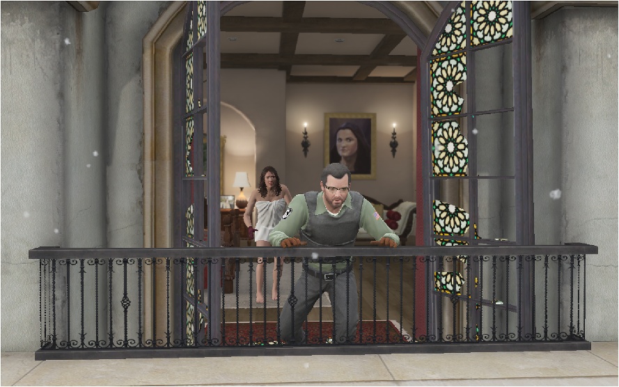
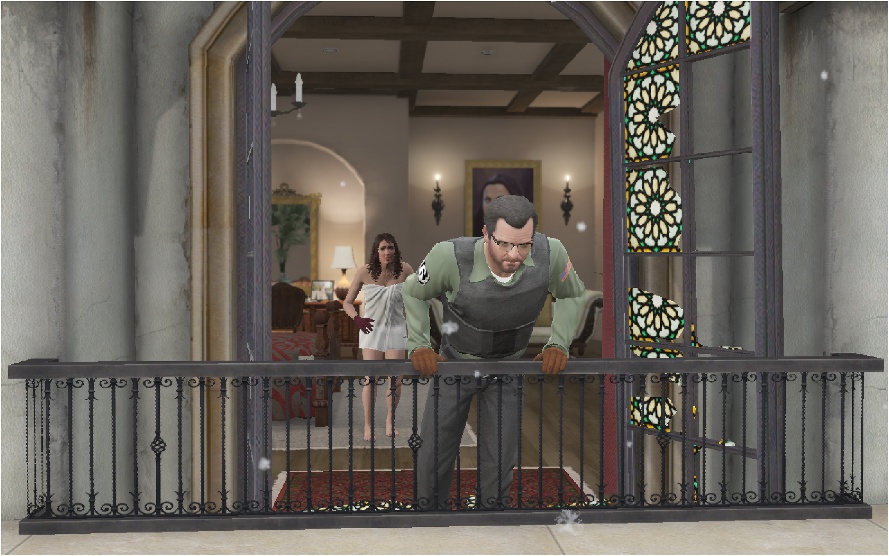
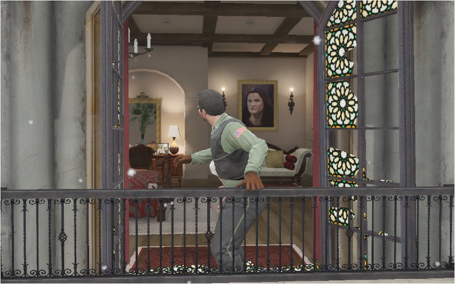
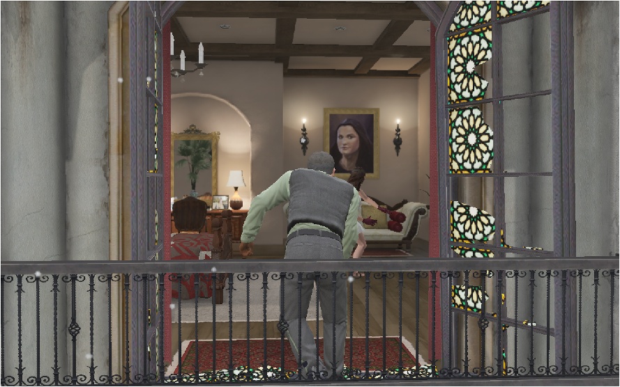
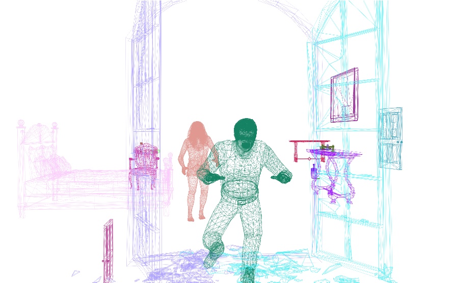
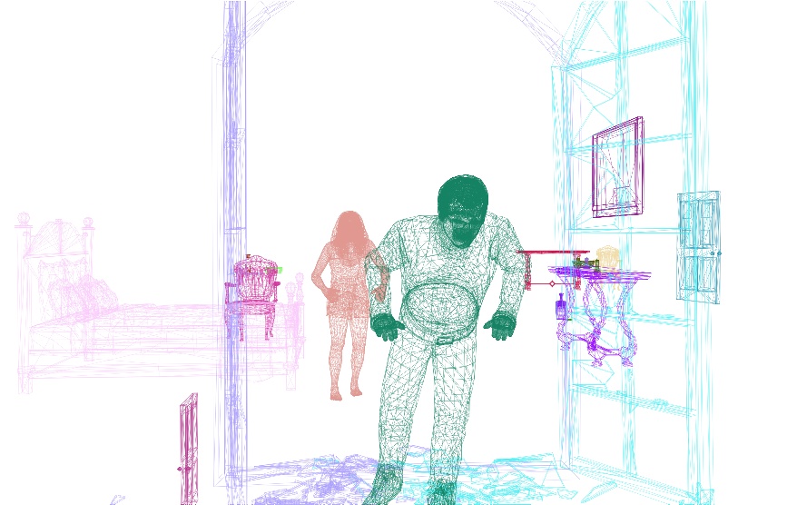
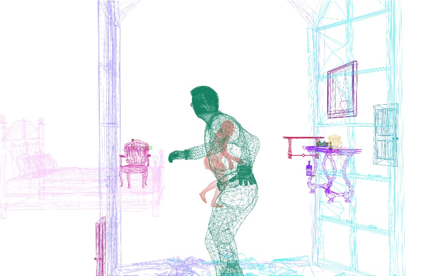
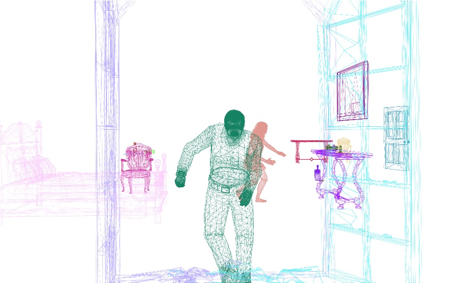
Figure 1: Temporal information in videos provides a lot of cues for 3D mesh reconstruction. For instance, as the main character in this scene turns we can accurately reconstruct both the front and back. Unfortunately, existing image-based datasets don’t permit to develop such methods. To alleviate this we introduce the synthetic SAIL-VOS 3D dataset and develop first baselines for this task.

1 Introduction

Understanding the 3D shape of an observed object over time is an important goal in computer vision. Very early work towards this goal [44, 43, 42] focused on recovering lines and primitives like triangles, squares and circles in images. Due to many seminal contributions, the field has significantly advanced since those early days. Given a single image, exciting recent work [31, 76, 37, 21] detects objects and infers their detailed 3D shape. Notably, the shapes are significantly more complex than the early primitives.

To uncover the 3D shape, recently, single view 3D shape reconstruction [77, 41, 55, 81, 48, 16, 10, 56] has garnered much attention. The developed data-driven and learning-based approaches achieve realistic reconstructions by inferring the 3D geometry and structure of objects. All those methods have in common the use of a single input image. However, moving objects and temporal information are not considered. Intuitively, as illustrated in fig:teaser, we expect temporal information to aid 3D shape reconstruction. How can methods benefit from complementary information available in multiple views?

Table 1: Comparisons of SAIL-VOS 3D and other 3D datasets.

	ShapeNet [7]	ModelNet [82]	PartNet [48]	SUNCG [69]	IKEA [39]	Pix3D [71]	ScanNet [14]	PASCAL3D+ [84]	ObjectNet3D [83]	KITTI [20]	OASIS [8]	SAIL-VOS 3D
Type	Synthetic	Synthetic	Synthetic	Synthetic	Real	Real	Real	Real	Real	Real	Real	Synthetic
Image/Video	-	-	-	Image	Image	Image	Video	Image	Image	Video	Image	Video
Indoor/Outdoor	-	-	-	Indoor	Indoor	Indoor	Indoor	Both	Both	Outdoor	Both	Both
Dynamics	Static	Static	Static	Static	Static	Static	Static	Static	Static	Dynamic	Static	Dynamic
Background	Uniform	Uniform	Uniform	Cluttered	Cluttered	Cluttered	Cluttered	Cluttered	Cluttered	Cluttered	Cluttered	Cluttered
# of Images	-	-	-	130,269	759	10,069	2,492,518	30,362	90,127	41,778	140,000	237,611
Objects per Images	Single	Single	Single	Multiple	Single	Single	Multiple	Multiple	Multiple	Multiple	Multiple	Multiple
# of Categories	55	662	24	84	7	9	296	12	100	3	-	178
3D Annotation Type	3D model	3D model	3D model	Voxel, depth	3D model	3D model	Depth, 3D model	3D model	3D model	Point cloud	Normals, depth	3D model, depth
Amodal/Modal GT	Amodal	Amodal	Amodal	Amodal	Amodal	Amodal	Modal	Amodal	Amodal	Modal	Modal	Amodal
# of 3D Annotations	51,300	127,915	26,671	5,697,217	759	10,069	101,854	55,867	201,888	40,000	140,000	3,460,213

Classical multi-view 3D reconstruction [65, 18, 6] exploits the geometric properties exposed in multiple views. For instance, structure from motion algorithms, e.g., [65], infer the 3D shape using multi-view geometry [24]. However note that the assumption of a static scene in these classical methods is often violated in practice. Moreover, classical 3D reconstruction focuses on finding the 3D shape of observed object parts. Nonetheless it is important for methods to predict occluded parts of objects or to infer object extent beyond the observed view [53].

To achieve a more realistic and more detailed reconstruction we aim to leverage temporal information. For this we think ground-truth 3D mesh annotations for video-data are particularly helpful. Unfortunately, this form of annotated data is not available in existing datasets. This is not surprising as acquiring this form of data is very time-consuming and hence expensive. In addition, annotations of this form are often ambiguous due to occlusions. However, following recent work on amodal segmentation [27], we think photo-realistic renderings of assets in computer games could come to the rescue. To study this solution, in this paper, we collect SAIL-VOS 3D, a synthetic video dataset with frame-by-frame 3D mesh annotations for objects, ground-truth depth for scenes and 2D annotations in the form of bounding boxes, instance-level semantic segmentation and amodal segmentation. We think this data serves as a good test bed for 3D perception algorithms.

In order to deal with dynamics of 3D shapes, we propose to take the temporal information into account by developing a baseline model. Specifically, instead of refining a spherical shape we introduce a reference mesh which carries information from earlier frames.

Based on the collected SAIL-VOS 3D dataset and existing image datasets like Pix3D [71], we study the proposed method as well as recent techniques for 3D reconstruction of meshes from images. We illustrate the efficacy of the developed model and the use of temporal information on the collected SAIL-VOS 3D dataset. Using Pix3D [71] we demonstrate generality.

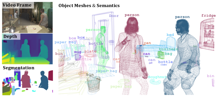
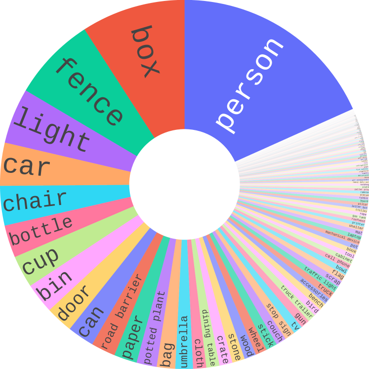
Categories

Occlusion Rate

Figure 2: The annotations of SAIL-VOS 3D include depth, instance-level modal and amodal segmentation, semantic labels and 3D meshes. On the right we show the statistics of the dataset in terms of numbers of objects in different categories and with different occlusion rate.

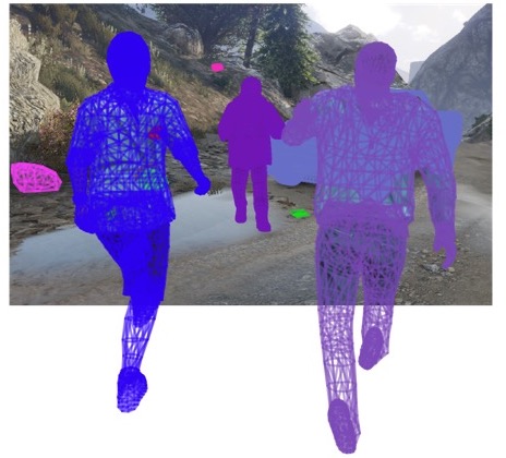
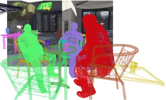
Figure 3: We overlay the RGB frame with the 3D mesh annotations. Note, the dataset contains annotations for partially observed objects including occluded and out-of-view objects. It is also a good benchmark for 2D/3D amodal perception.

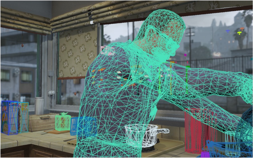
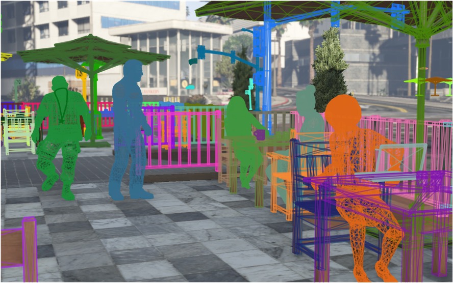
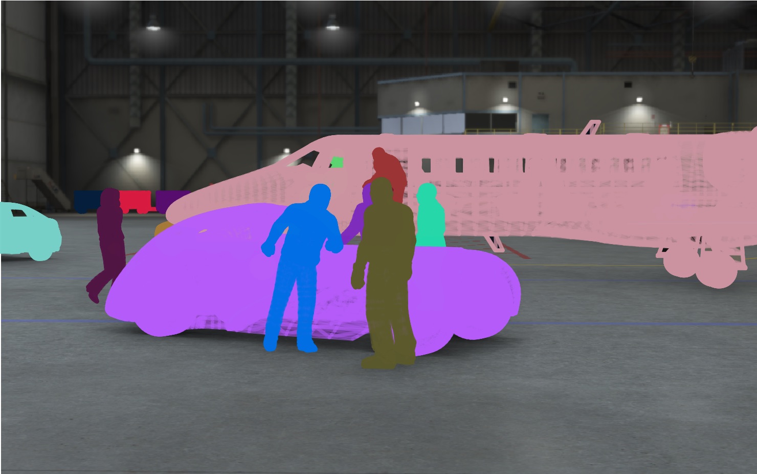
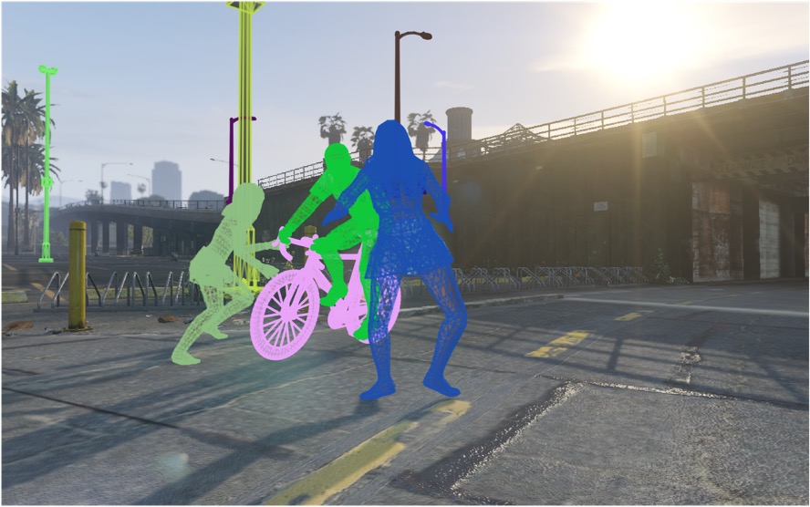
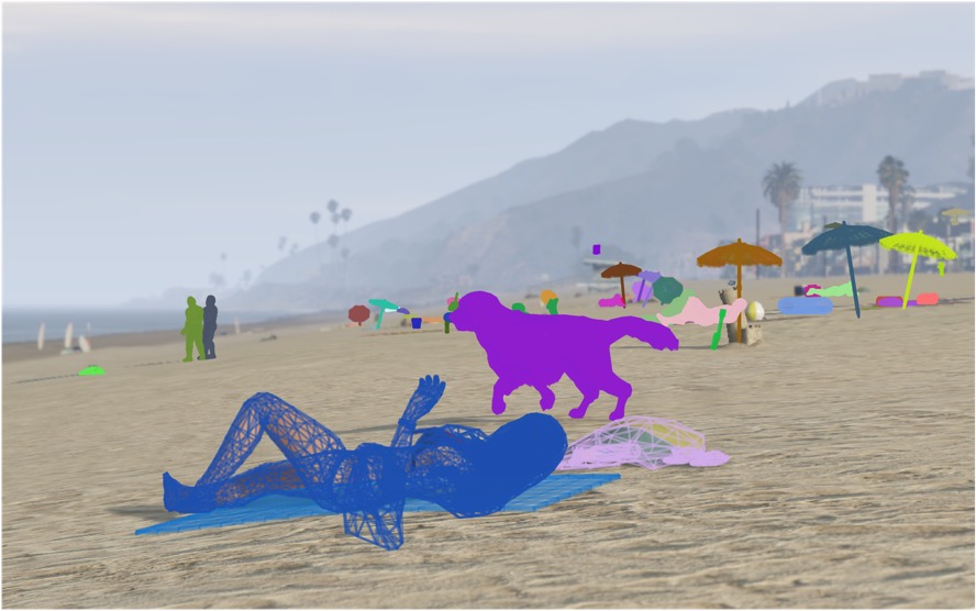
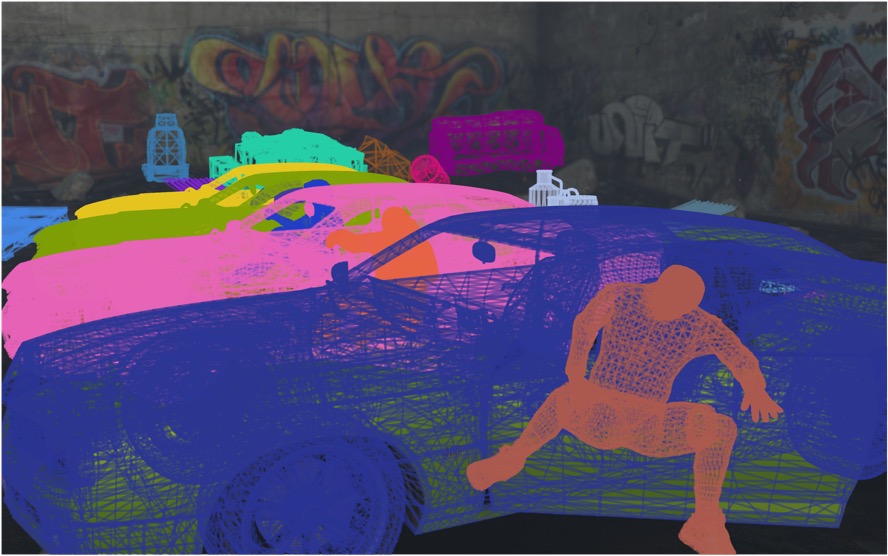
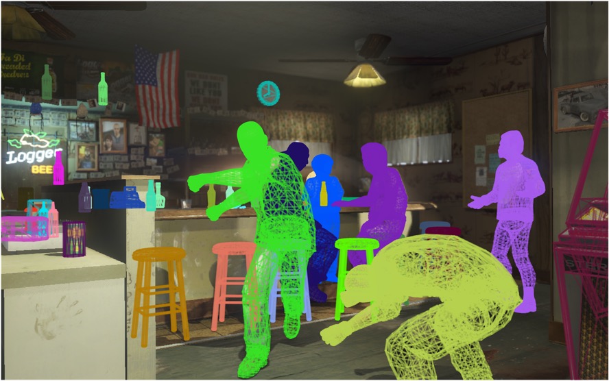
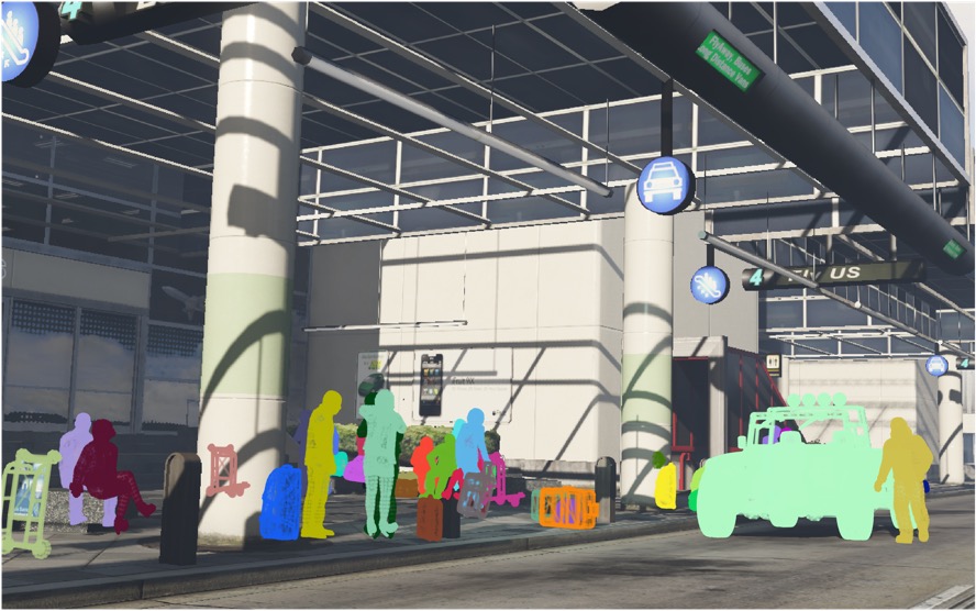
Figure 4: Example frames overlayed with 3D mesh annotations from SAIL-VOS 3D. We use different colors for different instances.

2 Related Work

Single-View Object Shape Reconstruction: Recently, a number of methods [77, 41, 47, 55, 81, 48, 15, 16, 10, 56, 31, 87, 76, 22, 37, 15, 80, 49, 47, 54] have been proposed for shape reconstruction from a single image. These approaches vary by their shape representation, e.g., meshes [77], occupancy grids [82], octrees [73], implicit fields [11, 47, 54] and point clouds [22]. Many of these methods assume that there is only a single shape to be reconstructed. Consequently, these methods usually use a curated datasets like ShapeNet [7], which contains only a single object at a time.

3D shape reconstruction methods that deal with multiple objects [31, 76, 37, 21] usually either involve a detection network [31, 37, 21] like Faster-RCNN [59], which has been very successful on 2D instance-level multi-object detection, or assume instance-level bounding boxes are given [76]. After obtaining the bounding boxes, the 3D shape of each instance is inferred within each bounding box. To generally deal with multiple objects, we also combine detection with shape reconstruction. However, instead of employing a single image, the proposed approach differs in our use of video data for reconstruction.

Multiple-View Object Shape Reconstruction: 3D understanding using multiple images has been studied and used for depth estimation [34, 74], scene reconstruction [51], semantic segmentation for 3D scenes [38], 3D object detection [68, 9, 50], and 3D object reconstruction [12, 85]. We focus on 3D object shape reconstruction literature here as it aligns with our goal. Traditional multi-view shape reconstruction approaches including structure from motion (SfM) [65] and simultaneous localization and mapping (SLAM) [18, 6] estimate 3D shapes from multiple 2D images using multi-view geometry [24]. However, these classical algorithms have well known constraints and are challenged by textureless objects as well as moving entities. Also, classical multi-view geometry does not infer the shape of unseen parts of an object.

Due to the success of deep learning, learning-based approaches to multi-view object 3D reconstruction [12, 85, 79, 75, 72, 5, 17, 33, 30, 26, 52] have received a lot of attention lately. Again, the majority of the aforementioned methods deal with only a single object. Dealing with instance-level multi-view reconstruction remains challenging as it requires not only object detection, but also object tracking as well as 3D shape estimation. Closer to the goal of our approach, SLAM-based methods have been proposed for object-level multi-view reconstruction [13, 64, 26, 70]. However, these methods are challenged by inaccurate estimation of camera poses and moving objects. In contrast, our approach aims at 3D understanding for dynamic objects.

3D Datasets: A number of 3D datasets have been introduced in recent years [66, 20, 36, 39, 84, 62, 7, 82, 83, 4, 28, 3, 69, 14, 46, 2, 71, 48, 8], all of which are commonly used for training, testing and evaluating 3D reconstruction algorithms. We summarize the properties of several common 3D datasets in tab:dataset. Datasets annotated on real world images [39, 71, 8, 84, 83] or videos [14, 20] are often small compared to synthetic datasets such as SUNCG [69]. Moreover, KITTI [20] and OASIS [8] contain only modal annotations, i.e., only visible regions are annotated. In order to create large scale datasets without labor-intensive annotation processes, synthetic 3D datasets [7, 69, 82] are useful.

Among those, ShapeNet [7] is one of the commonly used synthetic benchmarks for 3D reconstruction. However, the rendered images usually contain uniform backgrounds, making the distribution of rendered images very different from real world images. SUNCG [69] is one of the largest among the synthetic 3D datasets. However, the dataset contains static indoor scenes only, and doesn’t cover outdoor scenarios or dynamic scenes. In fact, except for KITTI [20], which contains dynamic scenes, i.e., moving objects with complex motion, to the best of our knowledge, there is no large scale 3D video dataset with instance-level 3D annotation that captures dynamic scenes with diverse scenarios.

Synthetic Datasets: Simulated worlds have been used for computer vision tasks such as optical flow [45], visual odometry [23, 60] and semantic segmentation [63] and human shape modeling [58, 86]. The game engine GTA-V has been used to collect large-scale data, e.g., for semantic segmentation [61, 60, 35], object detection [32], amodal segmentation [27], optical flow [60, 35] and human pose estimation [19].

3 SAIL-VOS 3D Dataset

For more accurate 3D video object shape prediction, we propose the SAIL-VOS 3D dataset: We collect an object-centric 3D video dataset from the photorealistic game engine GTA-V. The game engine simulates a three-dimensional world by modeling a real-life city. The resulting diverse object categories and the obtainable 3D structures make the game engine a suitable choice for collecting a large-scale 3D perception dataset.

As shown in fig:stats we collect the following data: video frames, camera matrices, depth data, instance level segmentation, instance level amodal segmentation and the corresponding 3D object shapes. Each instance is assigned a consistent id across frames.

3.1 Dataset Statistics

The presented SAIL-VOS 3D dataset contains 484 videos with a total of 237,611 frames at a resolution of 1280$\times$800. Note that each video may contain shot transitions. There are a total of 6,807 clips in the dataset and on average 34.6 frames per clip. The dataset is annotated with 3,460,213 object instances coming from 3,576 models, which we assign to 178 categories. To assign the categories, we use the SAIL-VOS labels [27]. There are 48 classes that overlap with the categories in the MSCOCO dataset [40]. fig:stats (right) shows the distribution of instances among the categories and their respective occlusion rate. Detailed statistics for clip length can be found in the Appendix.

We compare the proposed SAIL-VOS 3D dataset with other 3D datasets in tab:dataset. SUNCG [69], ScanNet [14], OASIS [8] and SAIL-VOS 3D are large scale datasets containing more than 100K images. In OASIS only visible parts of objects are annotated. In SUNCG and ScanNet static indoor scenes are used for collecting the datasets. In contrast, SAIL-VOS 3D contains moving objects, different scenarios (both indoor and outdoor with different lighting conditions and weather), and amodal 3D annotations. Compared to the commonly used ShapeNet [7], SAIL-VOS 3D contains images rendered with cluttered backgrounds and more object categories (178 vs. 55).

We show several annotated frames sampled from SAIL-VOS 3D in fig:outofview and fig:sailvos. Note, the dataset contains meshes despite occlusions, i.e., the entire shape is annotated even if part of it is out-of-view as shown in fig:outofview.

3.2 Dataset Collection Methodology

We collect the cutscenes in GTA-V following the work of Hu et al. [27]. Similarly, we alter the weather condition, the time of day and clothing of the characters to increase the diversity of the synthetic environment. However, different from their method, we are interested in capturing 3D information in the form of meshes, camera data, etc. This requires to extend the approach by Hu et al. [27], and we describe the details for obtaining the data in the following.

Meshes: The shapes of objects in GTA-V are all represented as meshes. In order to retrieve the meshes, we use GameHook [35] to hook into the Direct3D 11 graphics pipeline [1] which GTA-V employs. We first briefly highlight the key components of the Direct3D 11 graphics pipeline before we delve into details.

The Direct3D 11 graphics pipeline [1] consists of several stages which are traversed when rendering an image, e.g., the vertex shader stage, where vertices are processed by applying per-vertex operations such as coordinate transformations, the stream-output stage, where vertex data can be streamed to memory buffers, the rasterizer stage, where shapes or primitives are converted into a raster image (pixels), and the pixel shader stage, where shading techniques are applied to compute the color. The intermediate output of stages before the stream-output stage, e.g., the vertex shader stage, can not be directly copied to staging resources, i.e., resources which can be used to transfer data from GPU to CPU. This makes access to vertex data, and hence our approach, more complicated than earlier work: design of the graphics pipeline only permits access to vertex data via the stream-output stage.

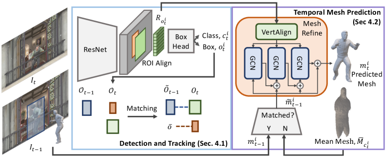
Figure 5: Video2Mesh: Mesh generation for the foreground person in frame $I_{t}$ using the boxed person in $I_{t-1}$ as a reference.

In GTA-V, the vertex shader stage processes object vertices by applying the camera matrices as well as the transformation matrices to animate articulated models. Our goal is to retrieve the output of the vertex shader stage which contains the meshes. Since the output of the vertex shader is not directly accessible, we need to retrieve it via the stream-output stage. For this we enable the stream-output stage by using a hook to alter the behavior of the Direct3D function CreateVertexShader. We ask it to not only create a vertex shader (it’s original behavior) but to additionally execute CreateGeometryShaderWithStreamOutput. This permits to append our own geometry shader whenever the vertex shader is created. Our geometry shader takes as input the output of the vertex shader. It doesn’t change the vertex data and directly writes the vertex data via the stream-output stage to a stream-output buffer. As this buffer is not CPU accessible, we subsequently copy the data to a staging resource so that it can be read by the CPU. We then store the vertex data, i.e., the meshes, using the OBJ file format.

Camera & Viewport: To obtain camera matrices we collect camera data from the constant buffers in the rendering pipeline. In each draw call, we store the world matrix, which transforms model coordinates to world coordinates, the view matrix, which transforms the world coordinates to camera coordinates, the projection matrix, which transforms the camera coordinates into image coordinates, as well as the viewport, which defines the viewing region in the rendering-device-specific coordinate.

Depth & Others: Along with the 3D shapes and camera matrices, we collect depth by copying the depth buffer from the rendering pipeline. We label shot transitions for each video. For each object in the dataset, we also collect additional information like the 2D segmentation, 2D amodal segmentation and 2D/3D human poses following Hu et al. [27].

4 Video2Mesh for 3D reconstruction

Given a video sequence $(I_{1},\ldots,I_{T})$ of $T$ frames, we are interested in inferring the set of meshes ${\cal M}_{t}$ for the existing objects in each frame $I_{t}$. A pictorial overview of our approach, Video2Mesh, is shown in fig:overview.

To infer the meshes, we first detect objects in each frame $I_{t}$. We let the unordered set ${\cal O}_{t}=\{o_{t}^{i}\}$ refer to the detected objects, i.e., $o_{t}^{i}$ is the $i^{\text{th}}$ detected object. Note that the set is unordered, i.e., $o_{t}^{i}$ and $o_{t-1}^{i}$ may not refer to the same object in frames $I_{t}$ and $I_{t-1}$. To establish object correspondence across time, we solve an assignment problem. This permits to use temporal information during shape prediction. Formally, for every frame $I_{t}$ we rearrange the objects ${\cal O}_{t-1}$ from the previous frame into the ordered tuple $\tilde{{\cal O}}_{t-1}^{t}=(\tilde{o}_{t-1}^{1},\ldots,\tilde{o}_{t-1}^{n_{t}})$, where $n_{t}=|{\cal O}_{t}|$. Specifically, for object $o_{t}^{i}$ from frame $I_{t}$ we let $\tilde{o}_{t-1}^{i}$ denote the corresponding object from frame $I_{t-1}$. If we cannot find a match in the previous frame, a special token is assigned to $\tilde{o}_{t-1}^{i}$.

With the objects tracked, we can use the prediction from the previous frame as a reference to predict meshes in the current frame. We detail detection and tracking in sec:detrack and explain the temporal mesh prediction in sec:cond.

4.1 Detection and Tracking

To obtain the set of objects ${\cal O}_{t}$ for frame $I_{t}$, we first use Faster-RCNN [59] to detect object bounding boxes and their class. Hence, each object $o_{t}^{i}=(b_{t}^{i},c_{t}^{i})$ consists of a bounding box and class estimate, i.e., $b_{t}^{i}$ and $c_{t}^{i}$. As previously mentioned, there are no correspondences for the detected objects between frames. To obtain those we solve an assignment problem.

Formally, given the detected objects from two consecutive frames, the assignment problem is formulated as follows:

$$\max_{{\bf A}_{t}} \sum_{i,j}{\bf A}_{t,ij}\left(\text{IoU}(b_{t}^{i},b_{t-1}^{j})-L(c_{t}^{i},c_{t-1}^{j})\right)$$

s.t. $${\bf A}_{t,ij}\in\{0,1\},\sum_{i}{\bf A}_{t,ij}\leq 1,\sum_{j}{\bf A}_{t,ij}=1.$$ (1)

Here, ${\bf A}_{t}\in\{0,1\}^{n_{t}\times n_{t-1}}$ is an assignment matrix, IoU is the intersection over-union distance between two bounding boxes and $L$ is the zero-one loss between two class labels. Intuitively, detected objects from two different frames will be matched if their bounding boxes are spatially close and their class labels are the same.

Given the assignment matrix ${\bf A}_{t}$, we align the objects of two frames as follows:

$$\begin{array}[]{ll}\tilde{o}_{t-1}^{i}\leftarrow o_{t-1}^{j},&\text{if}\;\;{\bf A}_{t,ij}=1\;\land\;\text{IoU}(b_{t}^{i},b_{t-1}^{j})>0.5,\\ \tilde{o}_{t-1}^{i}\leftarrow\bar{o},&\text{otherwise}.\end{array}$$ (4)

Here, $\bar{o}$ denotes a special token indicating that there were no matches. We don’t match objects if their IoU is too low.

4.2 Temporal Mesh Prediction

Our goal is to predict the set of meshes ${\cal M}=\{m_{t}^{i}\}$ for all objects $o_{t}^{i}\in{\cal O}_{t}$. In our case, each mesh $m_{t}^{i}$ is a triangular mesh, i.e., $m_{t}^{i}=(V_{t}^{i},F_{t}^{i})$ is characterized by a set of $K$ vertices $V_{t}^{i}\in\mathbb{R}^{K\times 3}$ and a set of triangle-faces $F_{t}^{i}\subseteq[1,\dots,K]^{3}$.

To predict a mesh $m_{t}^{i}$, we deform the vertices of a reference mesh $\tilde{m}_{t-1}^{i}$ based on the detected object’s ROI feature $R_{o_{t}^{i}}$ extracted from the image frame. The reference mesh $\tilde{m}_{t-1}^{i}$ is a class-specific mean mesh $\bar{M}_{c_{t}^{i}}$ if object $o_{t}$ is not tracked, and it is the predicted mesh $m_{t-1}^{i}$ from the previous frame if object $o_{t}$ is tracked. Formally,

$$\tilde{m}_{t-1}^{i}=\begin{cases}{\bf T}_{o_{t}^{i}}(\bar{M}_{c_{t}^{i}})&\text{if }\tilde{o}_{t-1}^{i}=\bar{o},\\ m_{t-1}^{i}&\text{otherwise}.\end{cases}$$ (5)

Recall, $\bar{o}$ is a special token indicating that there are no matches from the previous frame (see eq:trackassign). We use the transformation matrix ${\bf T}_{o_{t}^{i}}$ to align the mean mesh $\bar{M}_{c_{t}^{i}}$ with the reference frame of $o_{t}^{i}$. We parameterize ${\bf T}_{o_{t}^{i}}$ using a deep-net, which regresses the transformation matrix from the ROI features of $o_{t}^{i}$. Specifically, a mapping from $R_{o_{t}^{i}}$ to a rotation matrix with three degrees of freedom (the three Euler angles) is inferred. We do not consider translation here, as the mesh is centered in a bounding box.

Next, following prior work [77, 21] we refine the vertices of the reference mesh $\tilde{m}_{t-1}^{i}$ by performing $L$ stages of refinement using the MeshRefine procedure summarized in Module 1. Different from prior work, our reference mesh is propagated from the previous frames, i.e.,

$$\tilde{V}_{t}^{(l+1),i}={\tt MeshRefine}^{(l)}(R_{o_{t}^{i}},\tilde{V}_{t}^{(l),i}),$$ (6)

where $\tilde{V}_{t}^{(0),i}$ are the vertices of the reference mesh $\tilde{m}_{t-1}^{i}$. Finally, we use the original reference’s faces $\tilde{F}_{t-1}^{i}$ for the final mesh output, i.e.,

$$m_{t}^{i}=(V_{t}^{(L),i},\tilde{F}_{t-1}^{i}).$$ (7)

In greater detail, the MeshRefine procedure in Module 1 extracts image-aligned feature vectors for each vertex from an object’s ROI feature $R_{o_{t}^{i}}$ using the VertAlign operation [77, 21], where $E^{(l)}$ denotes the number of feature dimensions. Subsequently, a Graph Convolution Network (GCN) is used to learn a refinement offset $\Delta_{V}$ to update the reference vertices $\tilde{V}$. Finally, the module returns the updated mesh vertices to be processed in the next stage. In our case, we use $L=3$ and each $\text{GCN}^{(l)}$ consists of three GraphConv layers with ReLU non-linearity.

Input: ROI Feature $R$ and reference vertices $\tilde{V}$

$\phi_{V}={\tt VertAlign}({\tt Conv1x1}^{(l)}(R))\in\mathbb{R}^{K\times E^{(l)}}$

$\Delta_{V}={\tt GCN}^{(l)}(\text{Concat}(\phi_{V},\tilde{V}))\in\mathbb{R}^{K\times 3}$

Return: $\tilde{V}+\Delta_{V}$

Module 1 $\tt{MeshRefine}^{(l)}(R,\tilde{V})$

Table 2: Performance on SAIL-VOS 3D. Following MeshR-CNN [21] we report box AP, mask AP, and mesh AP.

%	All			Small Objects			Medium Objects			Large Objects
	$\text{AP}^{\text{box}}$	$\text{AP}^{\text{mask}}$	$\text{AP}^{\text{mesh}}$	$\text{AP}^{\text{box}}$	$\text{AP}^{\text{mask}}$	$\text{AP}^{\text{mesh}}$	$\text{AP}^{\text{box}}$	$\text{AP}^{\text{mask}}$	$\text{AP}^{\text{mesh}}$	$\text{AP}^{\text{box}}$	$\text{AP}^{\text{mask}}$	$\text{AP}^{\text{mesh}}$
Pixel2Mesh$\dagger$	25.29	23.08	8.96	6.47	3.81	2.30	21.72	19.64	10.73	44.35	43.78	19.09
Pix2Vox$\dagger$			6.62			2.81			7.51			16.56
MeshR-CNN [21]			9.68			2.53			10.35			20.80
Video2Mesh (Ours)			10.21			2.93			9.78			22.56

%	Slightly Occluded			Heavily Occluded			Short Clips			Long Clips
	$\text{AP}^{\text{box}}$	$\text{AP}^{\text{mask}}$	$\text{AP}^{\text{mesh}}$	$\text{AP}^{\text{box}}$	$\text{AP}^{\text{mask}}$	$\text{AP}^{\text{mesh}}$	$\text{AP}^{\text{box}}$	$\text{AP}^{\text{mask}}$	$\text{AP}^{\text{mesh}}$	$\text{AP}^{\text{box}}$	$\text{AP}^{\text{mask}}$	$\text{AP}^{\text{mesh}}$
Pixel2Mesh$\dagger$	30.10	29.90	12.44	16.27	13.04	2.21	29.38	26.85	12.92	23.33	22.74	8.43
Pix2Vox$\dagger$			9.31			2.80			9.05			6.80
MeshR-CNN [21]			12.66			3.34			13.39			9.03
Video2Mesh (Ours)			13.58			3.62			12.85			9.26

Table 3: Ablation study of our method. “MS”: mean shape. “T”: estimate ${\bf T}$ (sec:cond). “Temp.”: temporal prediction (sec:cond).

	MS	T	Temp.	$\text{AP}^{\text{box}}$	$\text{AP}^{\text{mask}}$	$\text{AP}^{\text{mesh}}$
1)	-	-	-	25.29	23.08	8.96
2)	✓	-	-	25.29	23.08	9.23
3)	✓	✓	-	25.29	23.08	9.66
4)	✓	✓	✓	25.29	23.08	10.21

[21]
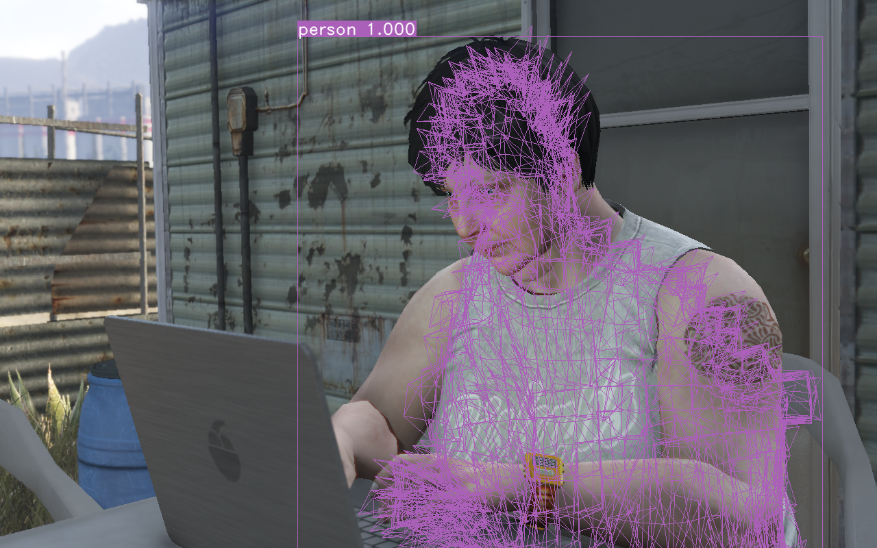
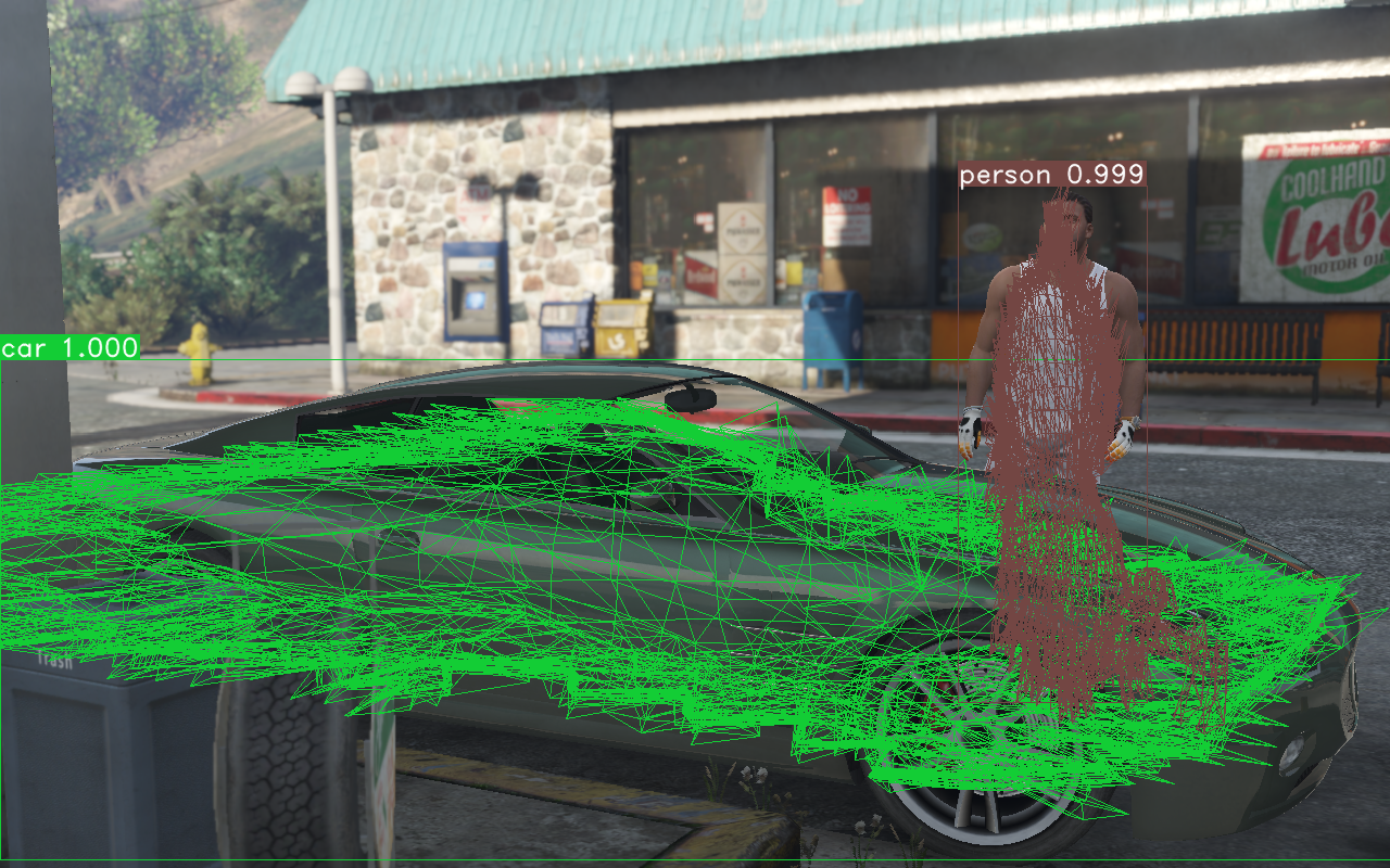
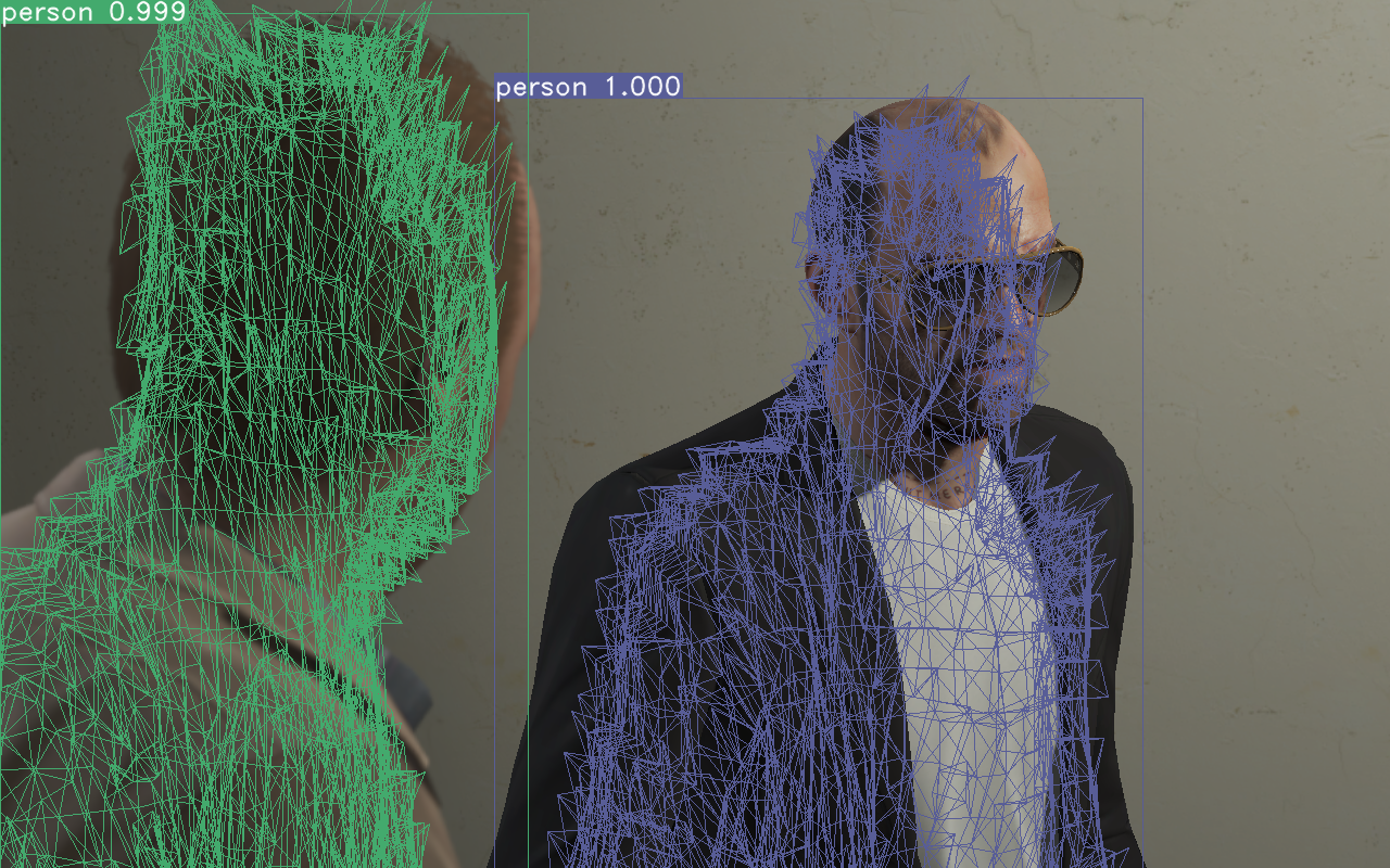
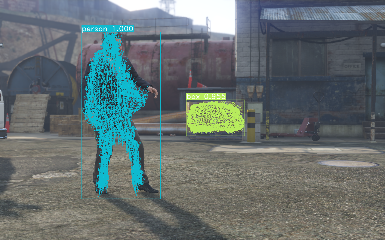
Ours

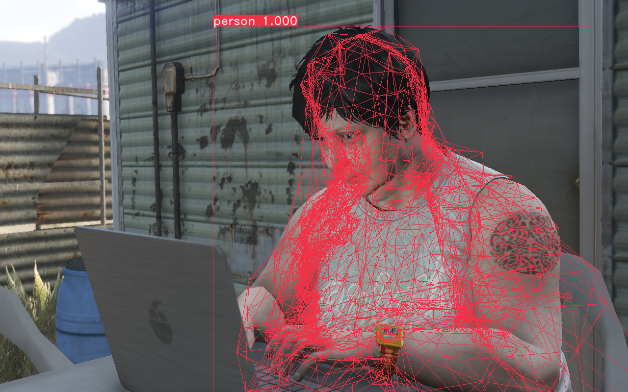
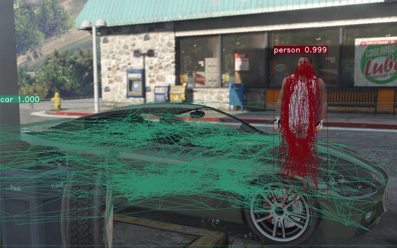
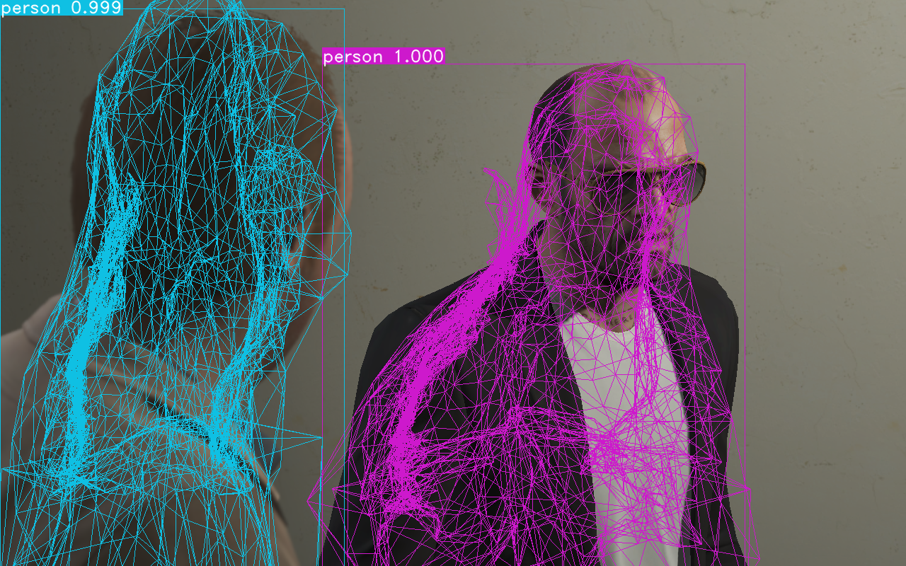
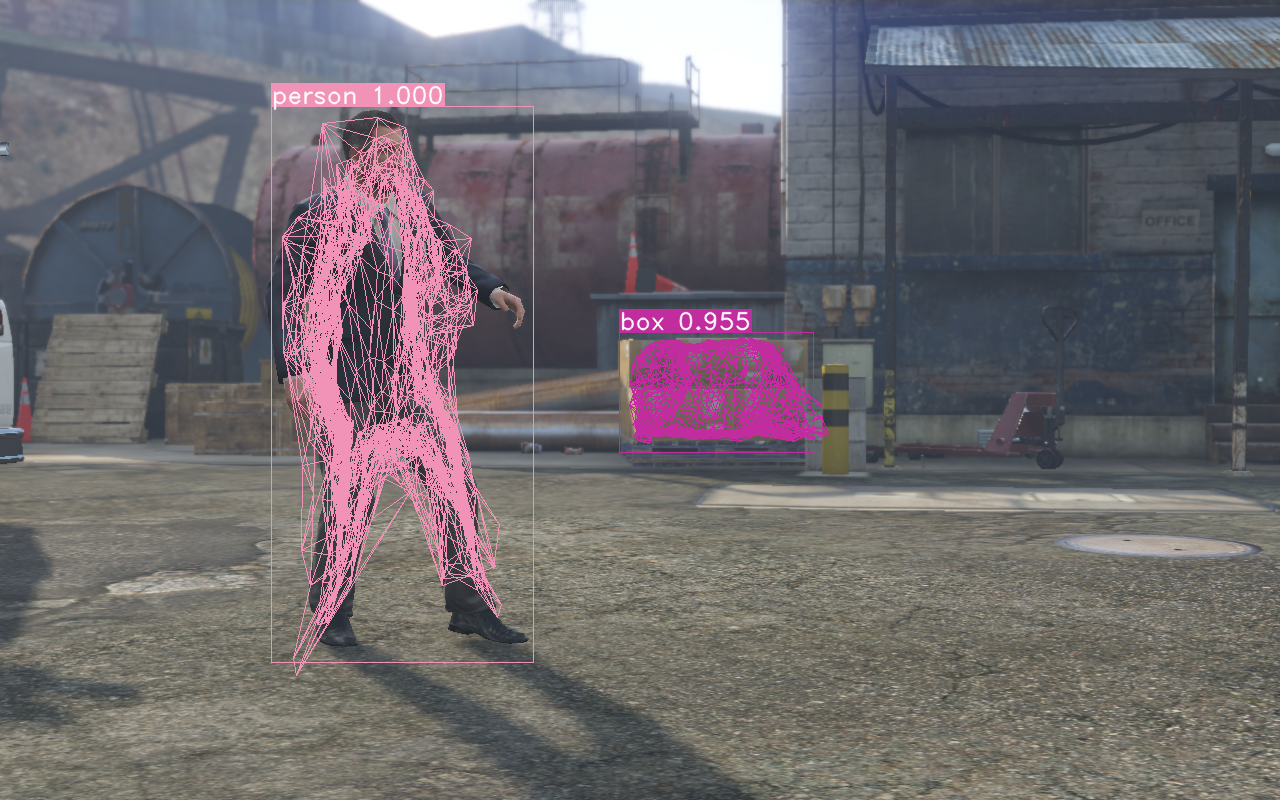
Figure 6: Visualization of 3D reconstructions on SAIL-VOS 3D.

Importantly, and different from prior work, instead of predicting meshes from a sphere [77], our approach depends on an additional time dependent reference mesh $\tilde{m}_{t-1}^{i}$. This reference $\tilde{m}_{t-1}^{i}$ summarizes information about an object $o_{t}^{i}$ obtained from the previous frame $I_{t-1}$. This enables a recurrent formulation suitable for mesh generation from videos by incorporating temporal information.

4.3 Training

We train our model using the dataset discussed in sec:data which consists of sequences of image frames, object bounding box annotations, class labels, and corresponding meshes. In the following, we discuss the training details abstractly and leave specifics to Appendix sec:supp_details.

To train the model parameters for mesh prediction, we use a gradient-based method to minimize the mesh loss based on differentiable mesh sampling [67]. The loss includes the Chamfer and normal distance between two sets of sampled points each from the prediction and ground-truth mesh. Minimizing the mesh loss encourages the predicted meshes to be similar to the ground-truth mesh. The training of bounding-boxes follows the standard Mask-RCNN procedure [25].

Different from standard end-to-end training, our training procedure consist of two stages:
Stage 1: We first pre-train the mesh refinement without taking temporal information into account. This is done by setting the reference mesh $\tilde{m}_{t-1}^{i}={\bf T}_{o_{t}^{i}}(\bar{M}_{c_{t}^{i}})$ $\forall\tilde{o}_{t-1}^{i}$.

Stage 2: We fine-tune our model to incorporate the temporal information of the reference mesh following eq:reference. Note that at training time, we do not unroll the recursion which would be computationally expensive. Instead, we use an augmented ground-truth mesh of $o_{t}^{i}$ as an approximation. This is done by randomly rotating the mesh and adding Gaussian noise to the vertices. Without the augmentation, the ground-truth mesh will not resemble $\tilde{m}_{t-1}^{i}$ which leads to a mismatch at test time.

5 Experimental Results

In the following we first discuss the experimental setup, i.e., datasets, metrics and baselines. Afterwards we show quantitative and qualitative results on the proposed SAIL-VOS 3D dataset and the commonly used Pix3D dataset.

5.1 Experimental Setup

We use the proposed SAIL-VOS 3D dataset to study instance-level video object reconstruction. Please see sec:datastat for statistics of this data. We also evaluate on Pix3D [71] to assess the proposed method on real images.

Evaluation metrics: For evaluation we use metrics commonly employed for object detection. Specifically, we report the average precision for bounding box detection, i.e., $\text{AP}^{\text{box}}$, using an intersection over union (IoU) threshold of 0.5. We also provide the average precision for mask prediction, i.e., $\text{AP}^{\text{mask}}$, using an IoU threshold of 0.5.

Additionally, to evaluate 3D shape prediction we follow Gkioxari et al. [21] and compute the average area under the per-category precision-recall curve using F1@0.3 with a threshold of 0.5, which we refer to via $\text{AP}^{\text{mesh}}$. Note, we consider a predicted mesh a true-positive if its predicted label is correct, not a duplicate detection, and its F1@0.3 $\geq 0.5$. Here, F1@0.3 is the F-score computed using precision and recall. For this, precision is the percentage of points sampled from the predicted mesh that lie within a distance of 0.3 to the ground-truth mesh. Conversely, recall is the percentage of points sampled from the ground-truth mesh that lie within a distance of 0.3 to the prediction. For SAIL-VOS 3D, we rescale the meshes such that the longest edge of the ground-truth mesh is 5. For Pix3D, following [21], we rescale the meshes such that the longest edge of the ground-truth mesh is 10.

For more insights, we further evaluate the aforementioned metrics on subsets of the object instances. This includes a split based on objects’ sizes (small – area less than $32^{2}$, medium, and large – area greater than $96^{2}$). We also split the objects based on occlusion rate, i.e., an object is heavily occluded if its occlusion rate is greater than $25\%$, otherwise it’s slightly occluded. Finally, we split based on the length of the video clip, i.e., a clip is classified as long if the number of frames is more than 30, otherwise short.

Baselines: In addition to the developed method we study three baselines on the proposed SAIL-VOS 3D data:

MeshR-CNN [21] – a single-view multi-object baseline. Its output representation is a mesh but the intermediate result is a voxel representation.

Pixel2Mesh$\dagger$ – The original Pixel2Mesh [77] is a single-view single-object baseline. To deal with multiple objects we use Mask-RCNN and attach Pixel2Mesh as an ROI head. We refer to this adjustment via Pixel2Mesh$\dagger$. We use the implementation by Gkioxari et al. [21] for this extension. We also considered as a baseline Pixel2Mesh++ [78], a multi-view single-object method. The fact that it is a single-object method makes a simple extension challenging as we would need to incorporate a tracking procedure. Moreover, Pixel2Mesh++ assumes camera matrices to be known which is not always feasible.

Pix2Vox$\dagger$ – The original Pix2Vox [85] is a multi-view single-object baseline which uses a voxel representation. Similar to Pixel2Mesh$\dagger$, to enable multiple object reconstruction, we extend the original Pix2Vox by attaching it to a Mask-RCNN. Similar to Pixel2Mesh++ it is non-trivial to extend Pix2Vox to the multi-object setting. It would require to include object tracking.

Input

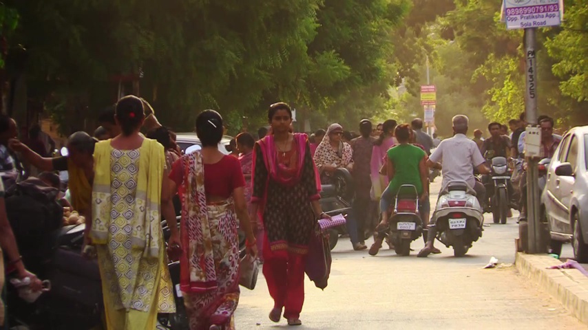
Predicted Shape

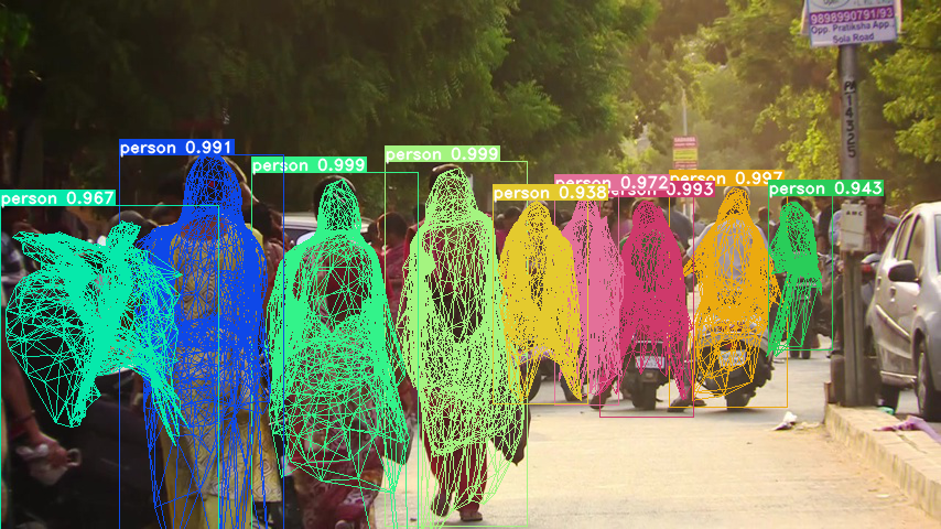
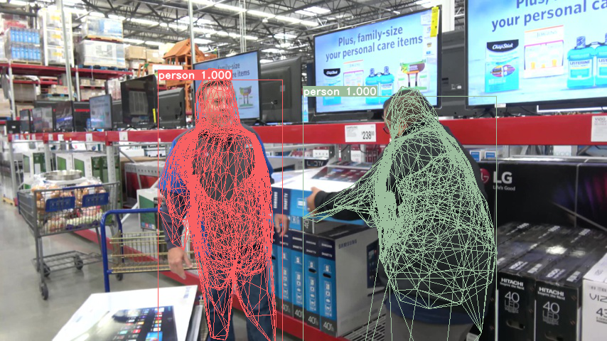
Figure 7: Predicted shapes of the SAIL-VOS 3D trained Video2Mesh model tested on DAVIS.

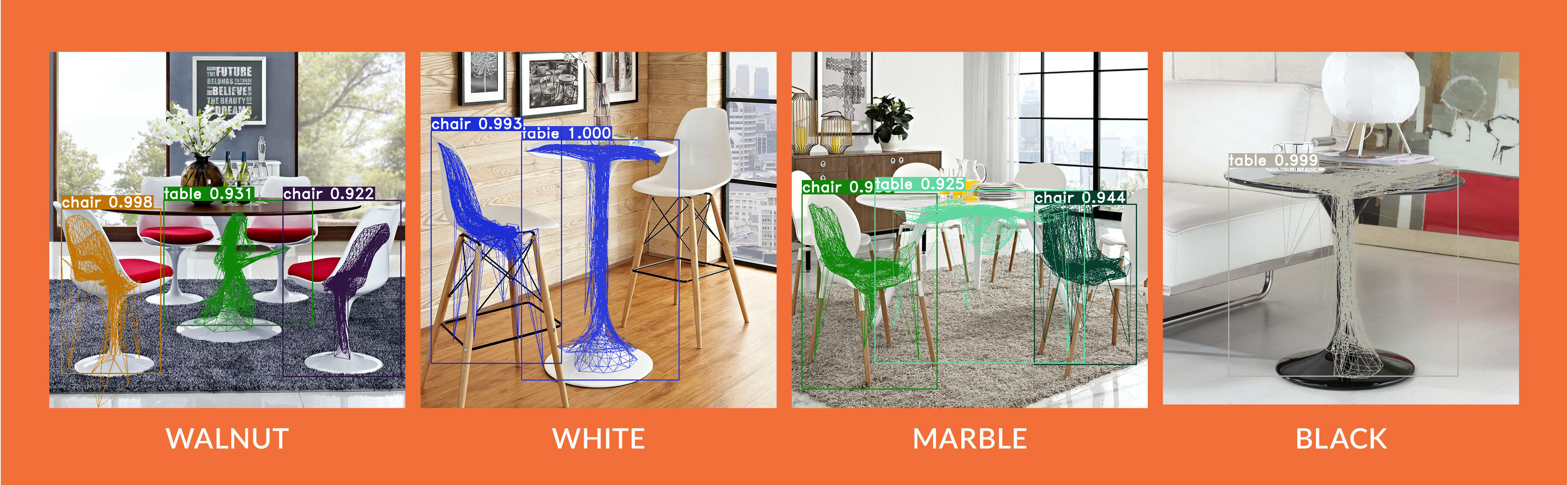
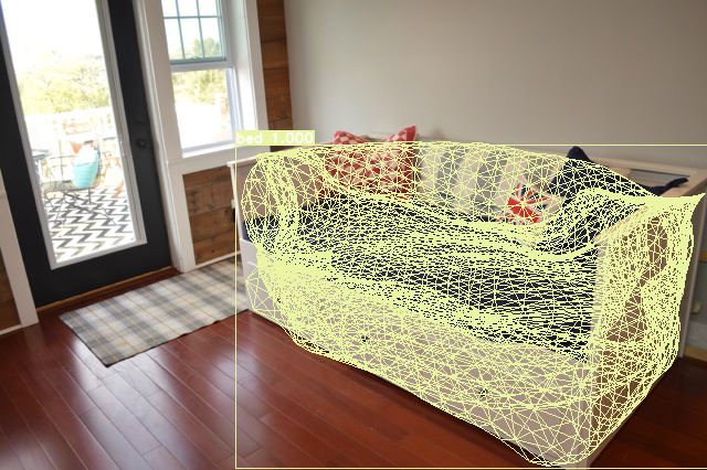
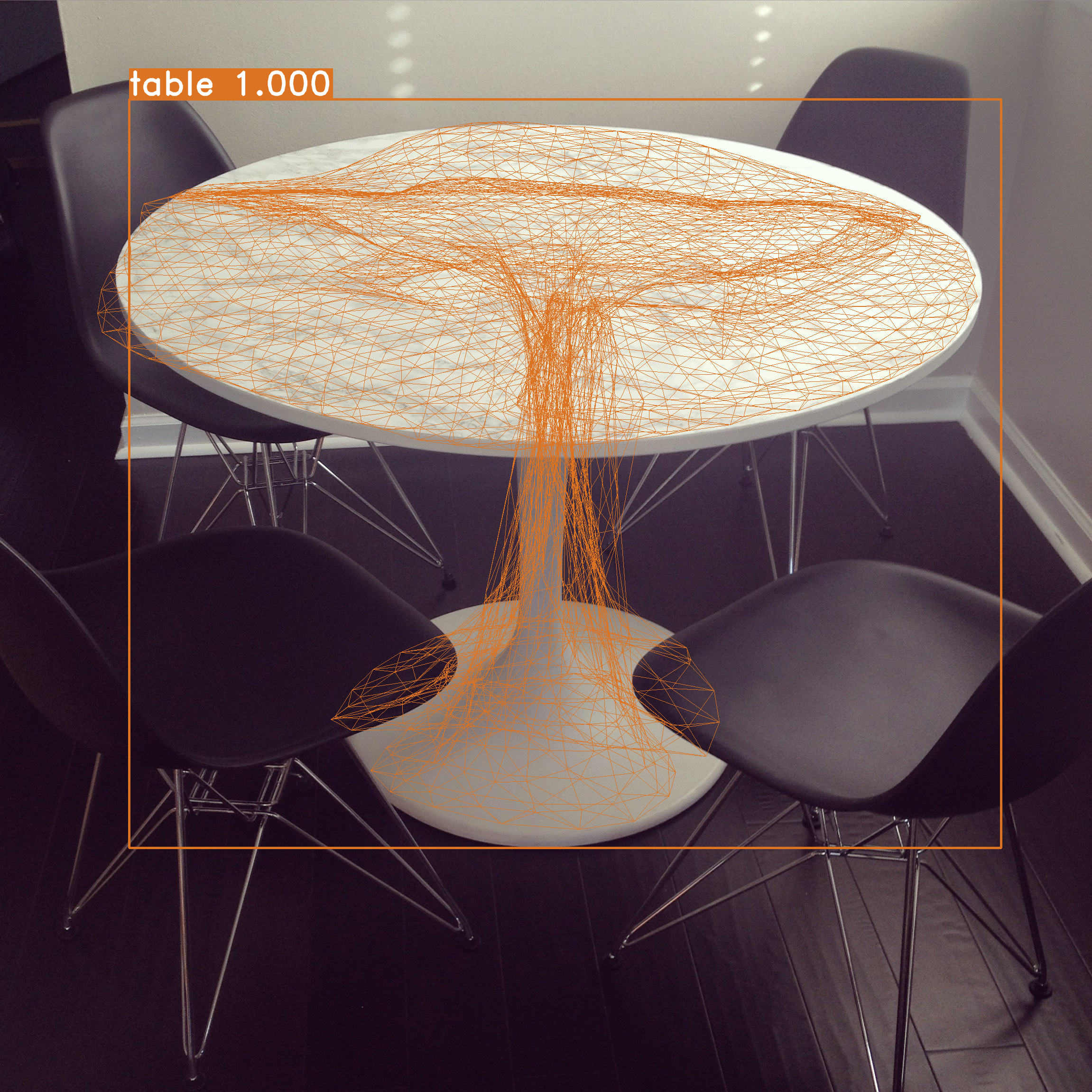
Figure 8: Visualization of 3D reconstructions from our Video2Mesh method on Pix3D.

5.2 SAIL-VOS 3D Dataset

SAIL-VOS 3D consists of 484 videos made up of 215,703 image frames. The data is split into 162 training videos (72,567 images, 754,895 instances) and 41 clips for validation (1,305 images, 12,199 instances). We leave the rest in test-dev/test-challenge sets for future use. Following Hu et al. [27] we use the 24 classes with an occlusion rate less than 0.75 for experimentation. To compute the mean shape, we average the occupancy grids in the object coordinate system over all the instances of a class using the training set. We binarize the averaged occupancy values, find the largest connected component, perform marching cubes to get the mesh, and simplify the mesh such that it contains about 4000 faces using [29].

Quantitative results: Quantitative results for the SAIL-VOS 3D dataset are provided in tab:exp. Note that we first train and fix the box and mask heads and then train different baselines for predicting meshes. On SAIL-VOS 3D we find that methods which predict shape via a mesh representation (Pixel2Mesh$\dagger$, MeshR-CNN, and our Video2Mesh) perform better than methods which predict using a voxel representation (Pix2Vox$\dagger$). We observe that our method outperforms the best baseline MeshR-CNN [21] in terms of $\text{AP}^{\text{mesh}}$. More notably, our method also outperforms baselines in slightly and heavily occluded subsets as well as long clips. This is to be expected, as our approach utilizes temporal information which helps to reason about occluded regions. To confirm this, we conduct an ablation study.

Ablation study: We study the importance of the mean shape (abbreviated via ‘MS’), whether to estimate transformation between mean shape and current frame (abbreviated via ‘T’) and the temporal prediction (abbreviated via ‘Temp.’). The results are summarized in tab:ablation. Note that we fix the box and mask head for this ablation study, which ensures a proper evaluation of our mesh head modifications. We observe use of the mean shape to lead to slight improvements (Row 2 vs. Row 1). Having transformation enabled improves results more significantly (Row 3 vs. Row 2), while the temporal prediction leads to further increase in performance (Row 4 vs. Row 3).

Qualitative results on SAIL-VOS 3D: Qualitative results are shown in fig:exp. We compare to the runner-up approach MeshR-CNN. Due to the use of a mean shape, we observe the 3D reconstructions of our method to be smoother.

Qualitative results on Real Data: We tested a SAIL-VOS 3D trained model (trained on person only) on a real video from the DAVIS dataset [57] and show a qualitative example in fig:davis. We find that predicted shapes are reasonable even though the model is trained on synthetic data.

6 Transferring to Pix3D

To assess the use of synthetic data we study transferability. Specifically, we use the SAIL-VOS 3D pretrained model and finetune on Pix3D [71] using different amounts of Pix3D training data. Pix3D [71] is an image dataset. Consequently, we cannot study temporal aspects of our model. We use as conditional input the mean shape rather than the prediction from the previous frame. For evaluation we follow Gkioxari et al. [21] and report the AP metrics in tab:transferring. More details regarding experimental setup and implementation are given in Appendix A. Qualitative results of our Video2Mesh method trained on all Pix3D data are provided in fig:shapenet.

In the low-data regime where only 10%, 20%, and 50% real mesh data (Pix3D) are available, pretraining on synthetic data is beneficial: the model pretrained on SAIL-VOS 3D outperfoms the model without pretraining. Note that depth data may also be a useful cue to facilitate transferability which we didn’t study yet.

Table 4: Results of transferring SAIL-VOS 3D to Pix3D ($\text{AP}^{\text{mesh}}$).

% of Pix3D data	10%	20%	50%	100%
Ours	9.0	16.8	36.6	43.7
Ours pretrained w/ SAIL-VOS 3D	16.4	22.5	38.0	42.8

7 Conclusion

We introduce SAIL-VOS 3D and develop a baseline for 3D mesh reconstruction from video data. In a first study we observe temporal data to aid reconstruction. We hope SAIL-VOS 3D facilitates further research in this direction.

Acknowledgements: This work is supported in part by NSF under Grant #1718221, 2008387, 2045586, MRI #1725729, and NIFA award 2020-67021-32799, UIUC, Samsung, Amazon, 3M, and Cisco Systems Inc. (Gift Award CG 1377144 - thanks for access to Arcetri).

Appendix: SAIL-VOS 3D: A Synthetic Dataset and Baselines for Object Detection and 3DMesh Reconstruction from Video Data

Appendix A Additional Details

Mesh loss: Recall, in sec:training we optimize the model parameters to minimize a mesh loss which encourages the predicted meshes to be similar to the ground-truth. In this section, we describe the details on how to compute this loss. Following Mesh R-CNN [21], the mesh loss is the sum of three distances, the Chamfer distance, the normal distance, and an edge regularizer, each of which we discuss in the following.

Given a predicted mesh $m_{t}^{i}$ and its corresponding ground-truth mesh $m_{t}^{i,*}$, differentiable sampling [67] is used to extract point clouds with normal vectors, $P$ and $P^{*}$, from each of the meshes. We sample 5,000 3D points from the meshes to compute the distances, i.e., $|P|=|P^{*}|=5000$ and for each point $p\in P$, $p^{\ast}\in P^{\ast}$ we have $p\in\mathbb{R}^{3}$ and $p^{\ast}\in\mathbb{R}^{3}$. We use those sets to compute the three losses as follows.

Chamfer distance:

$$L_{\text{cham}}(P,P^{*})=\frac{1}{|P|}\sum_{p\in P}\min_{p^{*}\in P^{*}}\left\lVert p-p^{*}\right\rVert^{2}+\frac{1}{|P^{*}|}\sum_{p^{*}\in P^{*}}\min_{p\in P}\left\lVert p^{*}-p\right\rVert^{2}.$$ (A8)

Normal distance:

$$L_{\text{norm}}(P,P^{*})=\frac{1}{|P|}\sum_{p\in P}\min_{p^{*}\in P^{*}}|\mathbf{u}_{p}^{\intercal}\mathbf{u}_{p^{*}}|+\frac{1}{|P^{*}|}\sum_{p^{*}\in P^{*}}\min_{p\in P}|\mathbf{u}_{p^{*}}^{\intercal}\mathbf{u}_{p}|,$$ (A9)

where $\mathbf{u}_{p}$ corresponds to the unit normal vector of a point $p\in P$ on a mesh surface.

Edge regularizer:

$$L_{\text{edge}}(V,E)=\frac{1}{|E|}\sum_{(v,v^{\prime})\in E}\left\lVert v-v^{\prime}\right\rVert^{2},$$ (A10)

where $V$ and $E\subseteq V\times V$ denote the set of vertices and edges of the predicted mesh. Here, $v\in V$ is a 3D vertex of the mesh.

The overall mesh loss for our model is a weighted sum of the Chamfer distance, normal distance, and edge regularizer on the predicted mesh at each stage of the mesh-refinement.

Mean mesh alignment: Recall, in eq:reference we introduce a transformation matrix $T_{o_{t}^{i}}$ to align the class-specific mean-mesh to the current object. More formally, we parameterize $T_{o_{t}^{i}}$ using a deep-net, which uses as input the ROI features $R_{o_{t}^{i}}$ and regresses to a rotation matrix with three degrees of freedom. We do not consider translation here, as the mesh is centered in a bounding box. To learn this transformation matrix, we train the parameters of $T_{o_{t}^{i}}$ to minimize the Chamfer distance and the normal distance between the mean-mesh and the ground-truth mesh. Note that we exclude the edge regularizer as a rotation maintains the edges’ length.

Bounding box depth extent prediction: We denote the depth extent via $dz$ and refer to the depth via $z_{c}$. We obtain both from the ground-truth mesh via

$$dz=z_{\text{far}}-z_{\text{near}},\quad z_{c}=\frac{(z_{\text{far}}+z_{\text{near}})}{2},$$ (A11)

where $z_{\text{far}}=\max_{v\in V}v_{z}$ and $z_{\text{near}}=\min_{v\in V}v_{z}$. Here, $v_{z}$ is the z-coordinate of vertex $v\in V$. Instead of predicting $dz$, following MeshR-CNN [21] we predict the scale normalized depth extent

$$\bar{dz}=\frac{dz}{z_{c}}\frac{f}{h},$$ (A12)

where $f$ is the focal length and $h$ is the height of the bounding box. Following Mesh R-CNN [21], we assume $z_{c}$ to be given during inference.

Implementation details: The model is optimized using SGD with a learning rate of 0.02 and momentum of 0.9. For SAIL-VOS 3D, we train each stage using 10,000 iterations . We use a batch size of 32 on 8 Tesla V100 GPUs. We use a ResNet-50 model pretrained on COCO for initialization of the backbone, RPN, the bounding box head and the mask head. For all the experiments on Pix3D, we use the COCO pretrained model as the initialization of the parameters in the backbone, RPN, the box head and the mask head except for the class-specific top layers. The parameters of the class-specific top layers are randomly initialized. For the experiments in  sec:transffering where we use the SAIL-VOS 3D pretrained model, we initialize the parameters in the mesh head from the SAIL-VOS 3D pretrained model.

Appendix B Statistics of Clip Length on SAIL-VOS 3D

In fig:clip, we plot the distribution of clip length of the SAIL-VOS 3D datasets. There are 6807 clips in total. There are around 14 clips per video. The average clip length is 34.6. Maximum clip length is 876 and minimum length is 1.

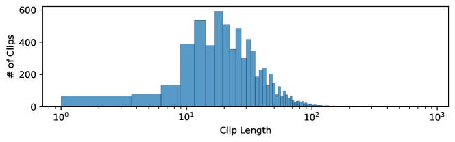
Figure A1: Clip length distribution of SAIL-VOS 3D dataset.

Appendix C More Qualitative Results

We present more qualitative results of the proposed Video2Mesh method on SAIL-VOS 3D in fig:supp_qual1. The video results are visualized in fig:supp_video. We use the same colors to highlight the tracked objects across frames. Our method can detect and track multiple instances in a video sequence as shown in fig:supp_video and reconstruct the 3D shapes as shown in fig:supp_qual1 and A3.

Input
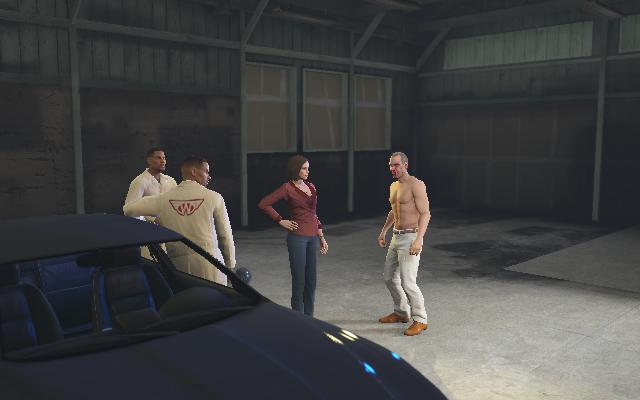
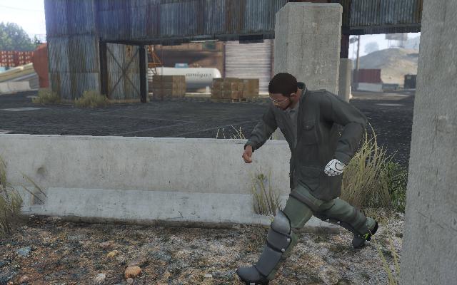
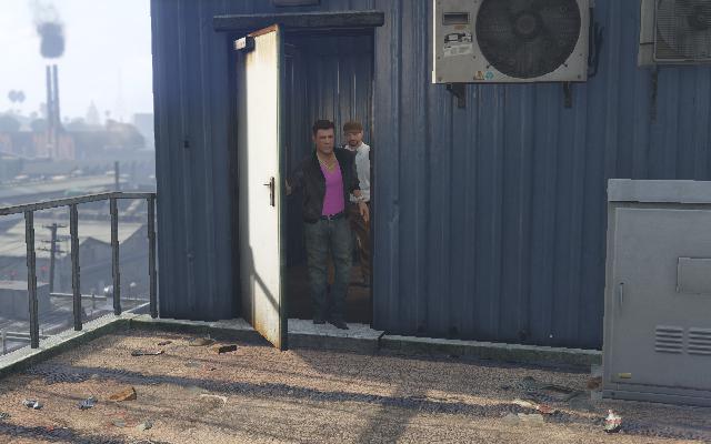
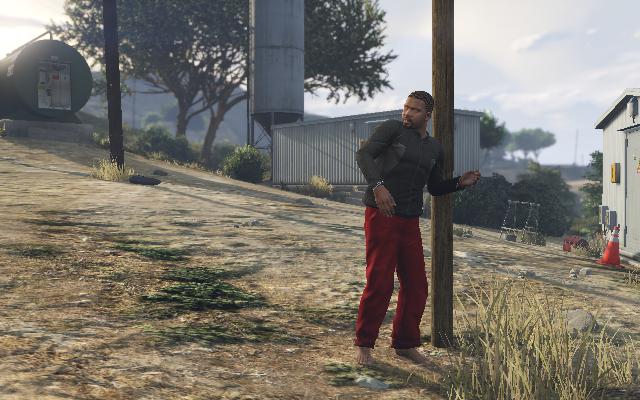
Results

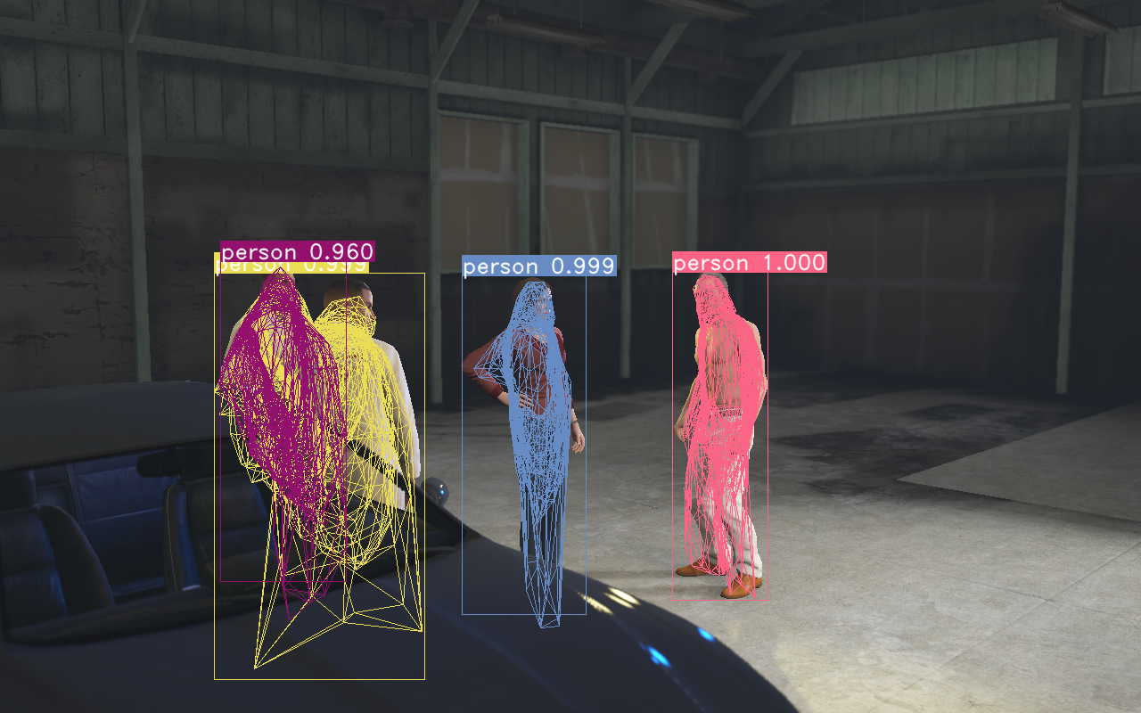
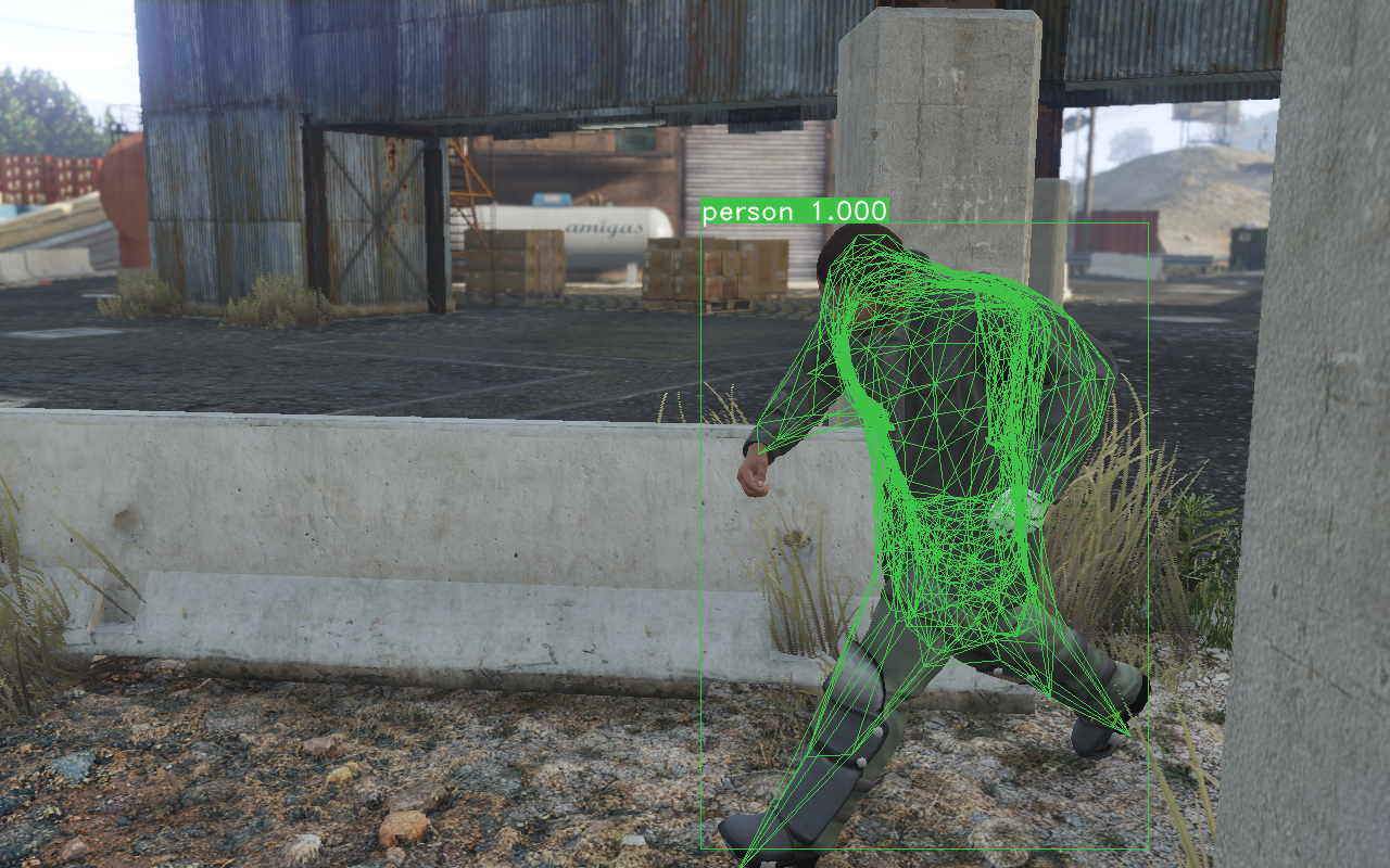
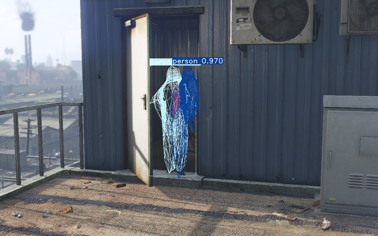
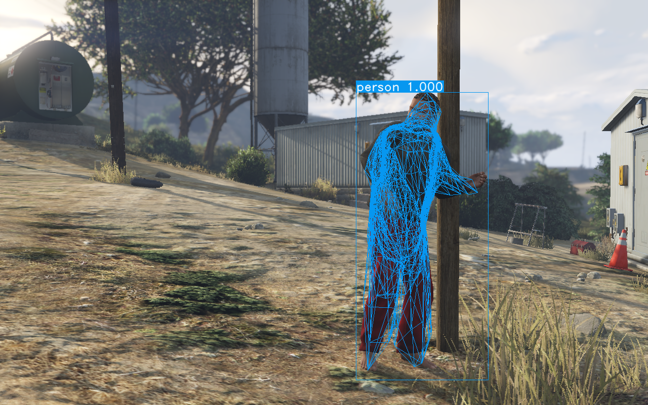
Figure A2: More qualitative results from Video2Mesh on SAIL-VOS 3D.

Input
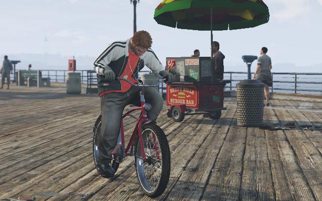
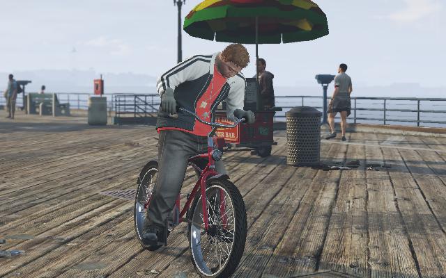
Results

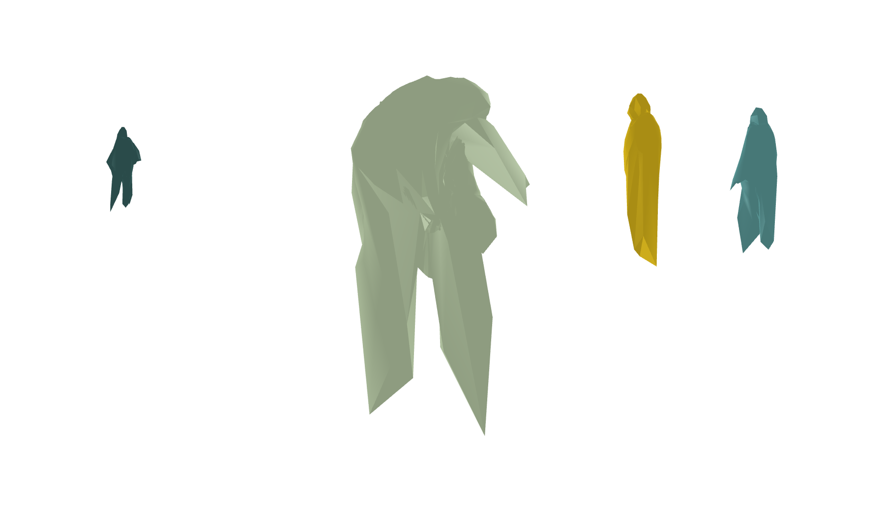
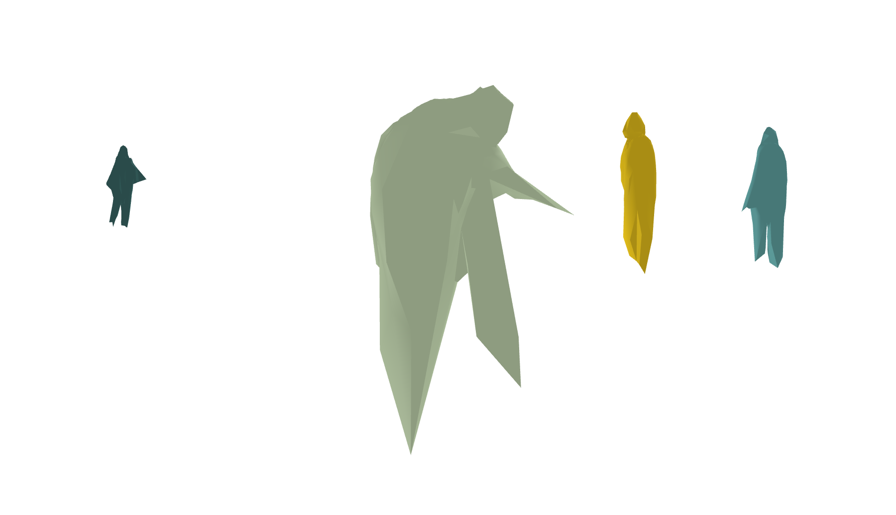
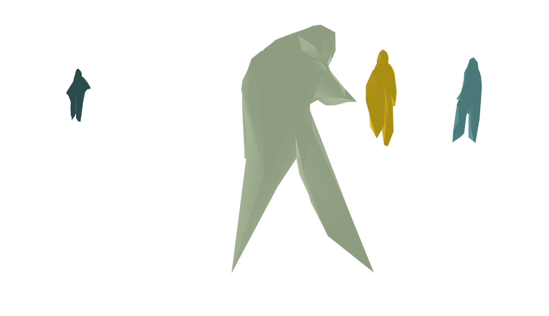
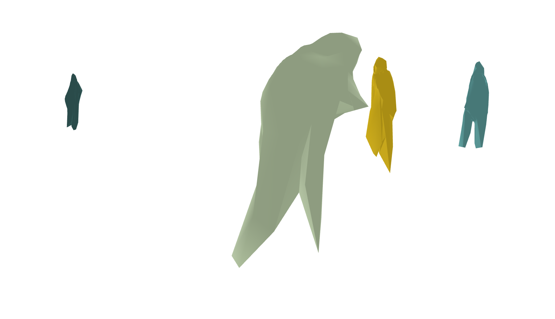
Figure A3: More qualitative results from Video2Mesh on SAIL-VOS 3D. We show a video sequence here.

References

- [1] Direct3d graphics pipeline. https://docs.microsoft.com/en-us/windows/win32/direct3d11/overviews-direct3d-11-graphics-pipeline.
- [2] Phil Ammirato, Patrick Poirson, Eunbyung Park, Jana Košecká, and Alexander C Berg. A dataset for developing and benchmarking active vision. In Proc. ICRA, 2017.
- [3] Iro Armeni, Sasha Sax, Amir R Zamir, and Silvio Savarese. Joint 2d-3d-semantic data for indoor scene understanding. arXiv preprint arXiv:1702.01105, 2017.
- [4] Iro Armeni, Ozan Sener, Amir R. Zamir, Helen Jiang, Ioannis Brilakis, Martin Fischer, and Silvio Savarese. 3d semantic parsing of large-scale indoor spaces. In Proc. CVPR, 2016.
- [5] Amir Arsalan Soltani, Haibin Huang, Jiajun Wu, Tejas D Kulkarni, and Joshua B Tenenbaum. Synthesizing 3d shapes via modeling multi-view depth maps and silhouettes with deep generative networks. In Proc. CVPR, 2017.
- [6] Tim Bailey and Hugh Durrant-Whyte. Simultaneous Localization and Mapping (SLAM): Part II. IEEE robotics & automation magazine, 2006.
- [7] Angel X Chang, Thomas Funkhouser, Leonidas Guibas, Pat Hanrahan, Qixing Huang, Zimo Li, Silvio Savarese, Manolis Savva, Shuran Song, Hao Su, et al. Shapenet: An information-rich 3d model repository. arXiv preprint arXiv:1512.03012, 2015.
- [8] Weifeng Chen, Shengyi Qian, David Fan, Noriyuki Kojima, Max Hamilton, and Jia Deng. OASIS: A Large-Scale Dataset for Single Image 3D in the Wild. In Proc. CVPR, 2020.
- [9] Xiaozhi Chen, Huimin Ma, Ji Wan, Bo Li, and Tian Xia. Multi-view 3d object detection network for autonomous driving. In Proc. CVPR, 2017.
- [10] Zhiqin Chen, Andrea Tagliasacchi, and Hao Zhang. Bsp-net: Generating compact meshes via binary space partitioning. In Proc. CVPR, 2020.
- [11] Zhiqin Chen and Hao Zhang. Learning implicit fields for generative shape modeling. In Proc. CVPR, 2019.
- [12] Christopher B Choy, Danfei Xu, JunYoung Gwak, Kevin Chen, and Silvio Savarese. 3D-R2N2: A unified approach for single and multi-view 3d object reconstruction. In Proc. ECCV, 2016.
- [13] Javier Civera, Dorian Gálvez-López, Luis Riazuelo, Juan D Tardós, and Jose Maria Martinez Montiel. Towards semantic slam using a monocular camera. In Proc. International Conference on Intelligent Robots and Systems, 2011.
- [14] Angela Dai, Angel X Chang, Manolis Savva, Maciej Halber, Thomas Funkhouser, and Matthias Nießner. Scannet: Richly-annotated 3d reconstructions of indoor scenes. In Proc. CVPR, 2017.
- [15] Angela Dai, Charles Ruizhongtai Qi, and Matthias Nießner. Shape completion using 3d-encoder-predictor cnns and shape synthesis. In Proc. CVPR, 2017.
- [16] Boyang Deng, Kyle Genova, Soroosh Yazdani, Sofien Bouaziz, Geoffrey Hinton, and Andrea Tagliasacchi. Cvxnet: Learnable convex decomposition. In Proc. CVPR, 2020.
- [17] Endri Dibra, Himanshu Jain, Cengiz Öztireli, Remo Ziegler, and Markus Gross. HS-Nets: Estimating human body shape from silhouettes with convolutional neural networks. In Proc. 3DV, 2016.
- [18] Hugh Durrant-Whyte and Bailey T. Simultaneous Localization and Mapping (SLAM): Part I. IEEE robotics & automation magazine, 2006.
- [19] Matteo Fabbri, Fabio Lanzi, Simone Calderara, Andrea Palazzi, Roberto Vezzani, and Rita Cucchiara. Learning to detect and track visible and occluded body joints in a virtual world. In Proc. ECCV, 2018.
- [20] Andreas Geiger, Philip Lenz, and Raquel Urtasun. Are we ready for autonomous driving? the kitti vision benchmark suite. In Proc. CVPR, 2012.
- [21] Georgia Gkioxari, Jitendra Malik, and Justin Johnson. Mesh R-CNN. In Proc. CVPR, 2019.
- [22] Thibault Groueix, Matthew Fisher, Vladimir G Kim, Bryan C Russell, and Mathieu Aubry. A papier-mâché approach to learning 3d surface generation. In Proc. CVPR, 2018.
- [23] Ankur Handa, Thomas Whelan, John McDonald, and Andrew J Davison. A benchmark for rgb-d visual odometry, 3d reconstruction and slam. In Proc. ICRA, 2014.
- [24] R. I. Hartley and A. Zisserman. Multiple View Geometry in Computer Vision. Cambridge University Press, 2004.
- [25] Kaiming He, Georgia Gkioxari, Piotr Dollár, and Ross Girshick. Mask R-CNN. In Proc. ICCV, 2017.
- [26] Lan Hu, Wanting Xu, Kun Huang, and Laurent Kneip. Deep-slam++: Object-level rgbd slam based on class-specific deep shape priors. arXiv preprint arXiv:1907.09691, 2019.
- [27] Y.-T. Hu, H.-S. Chen, K. Hui, J.-B. Huang, and A. G. Schwing. SAIL-VOS: Semantic Amodal Instance Level Video Object Segmentation – A Synthetic Dataset and Baselines. In Proc. CVPR, 2019.
- [28] Binh-Son Hua, Quang-Hieu Pham, Duc Thanh Nguyen, Minh-Khoi Tran, Lap-Fai Yu, and Sai-Kit Yeung. Scenenn: A scene meshes dataset with annotations. In Proc. 3DV, 2016.
- [29] Jingwei Huang, Hao Su, and Leonidas Guibas. Robust watertight manifold surface generation method for shapenet models. arXiv preprint arXiv:1802.01698, 2018.
- [30] Zeng Huang, Tianye Li, Weikai Chen, Yajie Zhao, Jun Xing, Chloe LeGendre, Linjie Luo, Chongyang Ma, and Hao Li. Deep volumetric video from very sparse multi-view performance capture. In Proc. ECCV, 2018.
- [31] Hamid Izadinia, Qi Shan, and Steven M Seitz. IM2CAD. In Proc. CVPR, 2017.
- [32] Matthew Johnson-Roberson, Charles Barto, Rounak Mehta, Sharath Nittur Sridhar, Karl Rosaen, and Ram Vasudevan. Driving in the matrix: Can virtual worlds replace human-generated annotations for real world tasks? In Proc. ICRA, 2017.
- [33] Abhishek Kar, Christian Häne, and Jitendra Malik. Learning a multi-view stereo machine. In Proc. NIPS, 2017.
- [34] Maria Klodt and Andrea Vedaldi. Supervising the new with the old: learning sfm from sfm. In Proc. ECCV, 2018.
- [35] Philipp Krähenbühl. Free supervision from video games. In Proc. CVPR, 2018.
- [36] Jonathan Krause, Michael Stark, Jia Deng, and Li Fei-Fei. 3D object representations for fine-grained categorization. In Proc. CVPR Workshops, 2013.
- [37] Abhijit Kundu, Yin Li, and James M Rehg. 3d-rcnn: Instance-level 3d object reconstruction via render-and-compare. In Proc. CVPR, 2018.
- [38] Abhijit Kundu, Xiaoqi Yin, Alireza Fathi, David Ross, Brian Brewington, Thomas Funkhouser, and Caroline Pantofaru. Virtual multi-view fusion for 3d semantic segmentation. In Proc. ECCV, 2020.
- [39] Joseph J Lim, Hamed Pirsiavash, and Antonio Torralba. Parsing ikea objects: Fine pose estimation. In Proc. ICCV, 2013.
- [40] Tsung-Yi Lin, Michael Maire, Serge Belongie, James Hays, Pietro Perona, Deva Ramanan, Piotr Dollár, and C Lawrence Zitnick. Microsoft coco: Common objects in context. In Proc. ECCV, 2014.
- [41] Jisan Mahmud, True Price, Akash Bapat, and Jan-Michael Frahm. Boundary-aware 3d building reconstruction from a single overhead image. In Proc. CVPR, 2020.
- [42] David Marr. Vision: A Computational Investigation into the Human Representation and Processing of Visual Information. MIT Press, 1982.
- [43] David Marr and Ellen C Hildreth. Theory of edge detection. In Proc. Royal Society of London, 1980.
- [44] David Marr and H. Keith Nishihara. Representation and recognition of the spatial organization of three-dimensional shapes. In Proc. Royal Society of London, 1978.
- [45] Nikolaus Mayer, Eddy Ilg, Philip Hausser, Philipp Fischer, Daniel Cremers, Alexey Dosovitskiy, and Thomas Brox. A large dataset to train convolutional networks for disparity, optical flow, and scene flow estimation. In Proc. CVPR, 2016.
- [46] John McCormac, Ankur Handa, Stefan Leutenegger, and Andrew J Davison. Scenenet rgb-d: Can 5m synthetic images beat generic imagenet pre-training on indoor segmentation? In Proc. ICCV, 2017.
- [47] Lars Mescheder, Michael Oechsle, Michael Niemeyer, Sebastian Nowozin, and Andreas Geiger. Occupancy networks: Learning 3d reconstruction in function space. In Proc. CVPR, 2019.
- [48] Kaichun Mo, Shilin Zhu, Angel X Chang, Li Yi, Subarna Tripathi, Leonidas J Guibas, and Hao Su. Partnet: A large-scale benchmark for fine-grained and hierarchical part-level 3d object understanding. In Proc. CVPR, 2019.
- [49] Charlie Nash, Yaroslav Ganin, SM Eslami, and Peter W Battaglia. PolyGen: An autoregressive generative model of 3d meshes. arXiv preprint arXiv:2002.10880, 2020.
- [50] Ahmed Samy Nassar, Sébastien Lefèvre, and Jan Dirk Wegner. Simultaneous multi-view instance detection with learned geometric soft-constraints. In Proc. ICCV, 2019.
- [51] Richard A Newcombe, Shahram Izadi, Otmar Hilliges, David Molyneaux, David Kim, Andrew J Davison, Pushmeet Kohi, Jamie Shotton, Steve Hodges, and Andrew Fitzgibbon. Kinectfusion: Real-time dense surface mapping and tracking. In IEEE International Symposium on Mixed and Augmented Reality, 2011.
- [52] Michael Niemeyer, Lars Mescheder, Michael Oechsle, and Andreas Geiger. Occupancy flow: 4d reconstruction by learning particle dynamics. In Proc. ICCV, 2019.
- [53] Stephen E Palmer. Vision science: Photons to phenomenology. MIT press, 1999.
- [54] Jeong Joon Park, Peter Florence, Julian Straub, Richard Newcombe, and Steven Lovegrove. Deepsdf: Learning continuous signed distance functions for shape representation. In Proc. CVPR, 2019.
- [55] Despoina Paschalidou, Luc Van Gool, and Andreas Geiger. Learning unsupervised hierarchical part decomposition of 3d objects from a single rgb image. In Proc. CVPR, 2020.
- [56] Songyou Peng, Michael Niemeyer, Lars Mescheder, Marc Pollefeys, and Andreas Geiger. Convolutional occupancy networks. In Proc. ECCV, 2020.
- [57] Jordi Pont-Tuset, Federico Perazzi, Sergi Caelles, Pablo Arbeláez, Alexander Sorkine-Hornung, and Luc Van Gool. The 2017 davis challenge on video object segmentation. arXiv:1704.00675, 2017.
- [58] Konstantinos Rematas, Ira Kemelmacher-Shlizerman, Brian Curless, and Steve Seitz. Soccer on your tabletop. In Proc. CVPR, 2018.
- [59] Shaoqing Ren, Kaiming He, Ross Girshick, and Jian Sun. Faster r-cnn: Towards real-time object detection with region proposal networks. In Proc. NIPS, 2015.
- [60] Stephan R Richter, Zeeshan Hayder, and Vladlen Koltun. Playing for benchmarks. In Proc. ICCV, 2017.
- [61] Stephan R Richter, Vibhav Vineet, Stefan Roth, and Vladlen Koltun. Playing for data: Ground truth from computer games. In Proc. ECCV, 2016.
- [62] Hayko Riemenschneider, András Bódis-Szomorú, Julien Weissenberg, and Luc Van Gool. Learning where to classify in multi-view semantic segmentation. In Proc. ECCV, 2014.
- [63] German Ros, Laura Sellart, Joanna Materzynska, David Vazquez, and Antonio M Lopez. The synthia dataset: A large collection of synthetic images for semantic segmentation of urban scenes. In Proc. CVPR, 2016.
- [64] Renato F Salas-Moreno, Richard A Newcombe, Hauke Strasdat, Paul HJ Kelly, and Andrew J Davison. Slam++: Simultaneous localisation and mapping at the level of objects. In Proc. CVPR, 2013.
- [65] Johannes L. Schönberger and Jan-Michael Frahm. Structure-from-motion revisited. In Proc. CVPR, 2016.
- [66] Nathan Silberman, Derek Hoiem, Pushmeet Kohli, and Rob Fergus. Indoor segmentation and support inference from rgbd images. In Proc. ECCV, 2012.
- [67] Edward Smith, Scott Fujimoto, Adriana Romero, and David Meger. Geometrics: Exploiting geometric structure for graph-encoded objects. In Proc. ICML, 2019.
- [68] Shiyu Song and Manmohan Chandraker. Joint sfm and detection cues for monocular 3d localization in road scenes. In Proc. CVPR, 2015.
- [69] Shuran Song, Fisher Yu, Andy Zeng, Angel X Chang, Manolis Savva, and Thomas Funkhouser. Semantic scene completion from a single depth image. In Proc. CVPR, 2017.
- [70] Edgar Sucar, Kentaro Wada, and Andrew Davison. Neural object descriptors for multi-view shape reconstruction. arXiv preprint arXiv:2004.04485, 2020.
- [71] Xingyuan Sun, Jiajun Wu, Xiuming Zhang, Zhoutong Zhang, Chengkai Zhang, Tianfan Xue, Joshua B Tenenbaum, and William T Freeman. Pix3d: Dataset and methods for single-image 3d shape modeling. In Proc. CVPR, 2018.
- [72] Maxim Tatarchenko, Alexey Dosovitskiy, and Thomas Brox. Multi-view 3d models from single images with a convolutional network. In Proc. ECCV, 2016.
- [73] Maxim Tatarchenko, Alexey Dosovitskiy, and Thomas Brox. Octree generating networks: Efficient convolutional architectures for high-resolution 3d outputs. In Proc. ICCV, 2017.
- [74] Zachary Teed and Jia Deng. DeepV2D: Video to depth with differentiable structure from motion. In Proc. ICLR, 2020.
- [75] Shubham Tulsiani, Alexei A Efros, and Jitendra Malik. Multi-view consistency as supervisory signal for learning shape and pose prediction. In Proc. CVPR, 2018.
- [76] Shubham Tulsiani, Saurabh Gupta, David F Fouhey, Alexei A Efros, and Jitendra Malik. Factoring shape, pose, and layout from the 2d image of a 3d scene. In Proc. CVPR, 2018.
- [77] Nanyang Wang, Yinda Zhang, Zhuwen Li, Yanwei Fu, Wei Liu, and Yu-Gang Jiang. Pixel2Mesh: Generating 3d mesh models from single rgb images. In Proc. ECCV, 2018.
- [78] Chao Wen, Yinda Zhang, Zhuwen Li, and Yanwei Fu. Pixel2mesh++: Multi-view 3d mesh generation via deformation. In Proc. ICCV, 2019.
- [79] Olivia Wiles and Andrew Zisserman. SilNet: Single-and multi-view reconstruction by learning from silhouettes. arXiv preprint arXiv:1711.07888, 2017.
- [80] Jiajun Wu, Yifan Wang, Tianfan Xue, Xingyuan Sun, Bill Freeman, and Josh Tenenbaum. Marrnet: 3d shape reconstruction via 2.5 d sketches. In Proc. NIPS, 2017.
- [81] Rundi Wu, Yixin Zhuang, Kai Xu, Hao Zhang, and Baoquan Chen. Pq-net: A generative part seq2seq network for 3d shapes. In Proc. CVPR, 2020.
- [82] Zhirong Wu, Shuran Song, Aditya Khosla, Fisher Yu, Linguang Zhang, Xiaoou Tang, and Jianxiong Xiao. 3d shapenets: A deep representation for volumetric shapes. In Proc. CVPR, 2015.
- [83] Yu Xiang, Wonhui Kim, Wei Chen, Jingwei Ji, Christopher Choy, Hao Su, Roozbeh Mottaghi, Leonidas Guibas, and Silvio Savarese. Objectnet3d: A large scale database for 3d object recognition. In Proc. ECCV, 2016.
- [84] Yu Xiang, Roozbeh Mottaghi, and Silvio Savarese. Beyond pascal: A benchmark for 3d object detection in the wild. In Proc. WACV, 2014.
- [85] Haozhe Xie, Hongxun Yao, Xiaoshuai Sun, Shangchen Zhou, and Shengping Zhang. Pix2Vox: Context-aware 3d reconstruction from single and multi-view images. In Proc. ICCV, 2019.
- [86] Luyang Zhu, Konstantinos Rematas, Brian Curless, Steven M Seitz, and Ira Kemelmacher-Shlizerman. Reconstructing nba players. In Proc. ECCV, 2020.
- [87] Chuhang Zou, Ersin Yumer, Jimei Yang, Duygu Ceylan, and Derek Hoiem. 3d-prnn: Generating shape primitives with recurrent neural networks. In Proc. ICCV, 2017.