eBASCS: Disentangling Overlapping Astronomical Sources II, using Spatial, Spectral, and Temporal Information

Abstract

The analysis of individual X-ray sources that appear in a crowded field can easily be compromised by the misallocation of recorded events to their originating sources. Even with a small number of sources, that nonetheless have overlapping point spread functions, the allocation of events to sources is a complex task that is subject to uncertainty. We develop a Bayesian method designed to sift high-energy photon events from multiple sources with overlapping point spread functions, leveraging the differences in their spatial, spectral, and temporal signatures. The method probabilistically assigns each event to a given source. Such a disentanglement allows more detailed spectral or temporal analysis to focus on the individual component in isolation, free of contamination from other sources or the background. We are also able to compute source parameters of interest like their locations, relative brightness, and background contamination, while accounting for the uncertainty in event assignments. Simulation studies that include event arrival time information demonstrate that the temporal component improves event disambiguation beyond using only spatial and spectral information. The proposed methods correctly allocate up to 65$\%$ more events than the corresponding algorithms that ignore event arrival time information. We apply our methods to two stellar X-ray binaries, UV Cet and HBC 515 A, observed with Chandra. We demonstrate that our methods are capable of removing the contamination due to a strong flare on UV Cet B in its companion $\approx$40$\times$ weaker during that event, and that evidence for spectral variability at timescales of a few ks can be determined in HBC 515 Aa and HBC 515 Ab.

1 Introduction

Analysis of X-ray data relies on the identification of the emitting sources and the allocation of the recorded events to the separated sources. When observing clusters of multiple contiguous sources, the presumable overlap of the sources’ point-spread functions (PSFs) casts uncertainty on the true origin of each of the recorded events, as well as on the physical and spectral properties of components in the observed system. These uncertainties are often amplified by issues such as low-count data and background contamination. One possible solution for analysis involves fitting multiple PSF components to binned images (Primini & Kashyap, 2014). However, X-ray data are originally acquired as event lists that allow high spatial resolution, and also contain energy and arrival time information that is lost when binned into a 2D image. The purpose of the separated extraction regions is to allow further processing and individual analysis of the separated sources. This is sub-optimal in the event of substantial overlap in the sources’ PSF, since events from each source are highly likely to contaminate the core of the other sources, which is expected to result in misclassification. For a given PSF size, this misclassification rate increases with both the size of the extraction region and the proximity of the sources. Moreover, events outside of the extraction regions are discarded from the analysis, which further inflates the uncertainties in parameter estimation due to the misclassification.

The problem with identification of sources in close pairs or in crowded fields is often encountered when running standard detection algorithms (e.g., wavdetect, Freeman et al., 2002) leading to source confusion and misclassification of extended sources. Source catalogs often flag problematic sources, use optical catalogs as a reference, or modify source and background extraction regions to exclude the overlapping part (Watson et al., 2009; Evans et al., 2010; Principe et al., 2017).

The limitations of the manual extraction approach have motivated the development of alternative algorithmic methodologies to tackle the problem of overlapping point sources in high-energy photon image analysis. Jones et al. (2015) developed a statistical approach to probabilistically allocate events to sources using spatial and spectral information. This method is known as Bayesian Separation of Close Sources (BASCS). BASCS models the spatial distribution using a known PSF and leverages the differences in the energy spectra of the components to estimate the locations of the point sources and their relative intensities. BASCS simultaneously provides the posterior distribution of the number of sources, which is particularly useful for detecting sources. This final feature of BASCS has added to the effort of probabilistic cataloging in dense fields that has been pursued by others (such as Portillo et al. (2017), whose method applies to multi-band optical data), but is not the focus of this article. More recently, Sottosanti et al. (2017) used a Bayesian mixture model to disentangle sources using spatial information, with the added feature of allowing for a diffuse non-isotropic background which is more suitable for $\gamma$-ray data. Picquenot et al. (2019) developed a method to separate extended sources from the background by using spectral information (unlike BASCS, this method uses binned images and assumes that the source components all have similar spectra). Foord et al. (2019) developed BayMAX, a statistical tool that uses spatial and spectral information to distinguish between single and dual active galactic nuclei (AGNs) via a Bayes Factor evaluation.

Here, we tackle the separate problem of time-variable sources. In many cases, temporal information carries significant discriminatory power, since astronomical objects display brightness and spectral variability. Their spectral energy distributions are also expected to change with source intensity. Therefore, we expect a method that leverages the temporal signatures of the observed sources to outperform existing algorithms in the task of allocating recorded events to temporally variable sources. The principles behind the methodology developed here follow those of Jones et al. (2015), but the variability of source intensity across time is incorporated into the model to aid in the task of source separation.

The paper is organized as follows. Section 2 provides an overview of the existing methodology and introduces the proposed methods. Section 3 presents the statistical analysis framework and computational procedures. Simulation studies are carried out in Section 4 to evaluate the performance of the methods. In Sections 5 and 6 two datasets from observations of the UV Cet and HBC 515 A systems (respectively) are analyzed. Finally, potential extensions and limitations are discussed in Section 7 and detailed results from our numerical studies appear in a number of appendices.

Symbol	Definition
$(x_{i},y_{i})$	Location of event $i$ on detector
$E_{i}$	Energy of event $i$
$t_{i}$	Event time of event $i$
$l_{i}$	Estimated wavelength of event $i$
$u_{j}=\{u_{j0},...,u_{jK}\}$	A collection of pre-selected $K+1$ breakpoints defining time bins for source $j$
$b_{ij}$	An indicator of time bin for event $i$ and source $j$,
	$b_{ij}=k$ if $t_{i}\in(u_{j,k-1},u_{jk}]$
$\mu_{j}$	True unknown location of source $j$ (2-D coordinates)
$f_{\mu_{j}}$	point spread function centered at $\mu_{j}$
$\theta_{jk}$	Spectral parameters for source $j$ and time bin $k$
$\theta_{j}$	Spectral parameters for source $j$ in BASCS algorithm
$E_{min},E_{max}$	Minimum and Maximum detected energy
$\pi_{j}$	Relative intensity of source $j$ ($j=0$ for background)
$S$	Number of Sources assumed
$s_{i}$	The true source of event $i$
$\lambda_{jk}$	Relative source intensity for source $j$ and time bin $k$
$n_{jk}$	True number of events detected for source $j$ and time bin $k$
$n_{j\cdot}$	True number of events detected for source $j$, i.e., $n_{j\cdot}=\sum_{k=1}^{K}n_{jk}$
$n_{\cdot k}$	Number of events detected for time bin $k$, i.e., $n_{\cdot k}=\sum_{j=1}^{S}n_{jk}$. These are
$n$	Total number of events detected, i.e., $n_{\cdot k}=\sum_{j,k}n_{jk}$
$(x,y,E,t,b)$	Vectors of the corresponding event specific variables

Table 1: Symbols used in this work.

2 Data and Statistical Models

2.1 Structure of the Data

High-energy detectors, such as Charged Coupled Device (CCD) imaging spectrometers, record detector spatial coordinates, $(x_{i},y_{i})$, arrival time, $t_{i}$, and energy, $E_{i}$. The full event list for $n$ recorded events is denoted as $\mathbf{x}=\{\mathbf{x}_{i}\}_{i=1}^{n}=\{(x_{i},y_{i},t_{i},E_{i})\}_{i=1}^{n}$. The observed spatial and spectral data is subject to the effect of the Point Spread Function (PSF) and the Redistribution Matrix Function (RMF). While the spatial dispersion of events by the PSF is explicitly accounted for in the model, for this study the RMF-induced energy dispersion is ignored and the observed spectra is modelled, rather than the source spectra.

Each recorded event is assumed to originate either from one of the sources located in the field of view, or from the background. In this article, only point sources are considered. Our proposed methods, unlike BASCS (Jones et al., 2015), assume that the number of observed sources on the image is known. The location, intensities, spectral distributions, and light curves are unknown. Background events are assumed to be uniformly distributed spatially under the source. Their spectrum is assumed to be known up to a normalization factor, and can be either uniform, or one of the models described in Section 2.4. We expect the modeling to be robust to mild deviations from the assumption of spatial uniformity of the background, as photons that are spatially distant from the sources are highly likely to be attributed to the background, irrespective of the background model.

2.2 Finite Mixture Model

A natural way to describe data assumed to originate from a collection of sub-populations (in this case, the sources and background) is with the class of statistical models known as finite mixture distributions. In such models, each event $\mathbf{x}_{i}$, $i=1,\dots,n$ is assumed to arise from one of $S+1$ ($S$ sources and the background) component distributions $\{h_{j}(\mathbf{x}_{i}|\Theta_{k})\}_{j=0}^{S}$, each parametrized by a parameter vector $\Theta_{k}$. It is further assumed that it is not known which mixture component generated each observation. The background contamination is defined as corresponding to component $j=0$ of the finite mixture. Further denote by $w_{j}$ the proportion of the population originated from mixture component $j$, so that $\sum_{j=0}^{S}w_{j}=1$. The likelihood of data $\mathbf{x}$ is thus:

$$p(\mathbf{x}_{i}|\Theta,\mathbf{w})=\sum_{j=0}^{S}w_{j}h_{j}(\mathbf{x}_{i}|\Theta_{j}).$$ (1)

With the aim of learning which mixture component underlies each observed event, we introduce the latent indicator variables, $s_{i}$, into the model: $s_{i}=j$ if $\mathbf{x}_{i}$ is drawn from mixture distribution $h_{j}$ i.e., if event $i$ originated from source $j$. Since $\mathbf{w}=(w_{0},\dots,w_{S})$ gives the proportion of the population of events belonging to each mixture, and $\mathbf{s}=(s_{1},\dots,s_{n})$ gives the mixture assignment of event $\mathbf{x}_{i}$, it is sensible to model $\mathbf{s}$ with a Multinomial distribution:

$$(s_{1},\dots,s_{n})\mid\mathbf{w}\sim\text{Multinomial}(n;(w_{0},\dots,w_{S})).$$ (2)

The joint distribution of the data, $\mathbf{x},$ and latent variable, $\mathbf{s}$, is then given by:

$$p(\mathbf{x},s|\Theta,\mathbf{w}) =p(\mathbf{s}|\mathbf{w})p(\mathbf{x}|\mathbf{s},\Theta)=\prod_{i=1}^{n}p(s_{i}|\mathbf{w})p(\mathbf{x}|s_{i},\Theta)$$

$$=\prod_{i=1}^{n}\prod_{j=0}^{S}p(s_{i}=j|w_{j})p(\mathbf{x}_{i}|s_{i}=j,\Theta_{j})$$

$$=\prod_{i=1}^{n}\prod_{j=0}^{S}w_{j}h_{j}(\mathbf{x}_{i}|\Theta_{j}).$$ (3)

For the rest of this article, we refer to the mixture weights, $\mathbf{w}$, as the relative intensities of the sources. Now that the general framework for statistical modelling of overlapping sources is established, models for the individual mixture distributions $\{h_{j}(\mathbf{x}_{i}|\Theta_{j})\}_{j=0}^{S}$ can be constructed. In particular, each component is a combination of sub-models for the spatial, spectral and temporal data. BASCS (Jones et al., 2015) only included $\{(x_{i},y_{i},E_{i})\}_{i=1}^{n}$, i.e., only the spatial and spectral information. The contribution to the existing framework is the formulation of a model for the temporal data $\{t_{i}\}_{i=1}^{n}$ and its integration into the current methodology.

2.3 Spatial Model

The detector spatial coordinates of an event $(x_{i},y_{i})$ are a deviation from the actual (unknown) position of the event’s originating source (say $j$), $\mu_{j}=(\mu_{xj},\mu_{yj})$. This deviation is due to the PSF, the response of the imaging system to the incident events that redistributes them on the surface of the detector according to a telescope and detector specific distribution centered at $\mu_{j}$. In our numerical studies, we assume that the PSF is well approximated by a King profile (see Appendix A and Jones et al., 2015). The observed event locations from source $j$ are, therefore, distributed according to the PSF centered at the unknown source location $\mu_{j}$, i.e.,

$$(x_{i},y_{i})\mid(s_{i}=j,\mu_{j})\sim f_{\mu_{j}}(x_{i},y_{i})$$ (4)

for $j=1,\dots,S$, where $f_{\mu_{j}}(x_{i},y_{i})$ denotes the PSF centered at $\mu_{j}$ evaluated at $(x_{i},y_{i})$.

As for the background, the assumption of spatial uniformity across the image means:

$$(x_{i},y_{i})\mid(s_{i}=0)\sim\text{Uniform.}$$ (5)

2.4 Spectral Model

In addition to spatial information, Jones et al. (2015) discuss the benefits of including spectral information when allocating events to sources. Generally, approximating the observed spectral energy distribution with a rough shape is a simple way to exploit spectral differences among sources, with relatively little additional computation. A simple sensible photon energy model is a Gamma distribution, because it only allows positive energy values and its mode is around the mid-to-low energy region. This yields:

$$E_{i}\mid(s_{i}=j,\alpha,\gamma)\sim\text{Gamma}(\alpha_{j},\alpha_{j}/\gamma_{j})$$ (6)

for $j=1,\dots,S$, where $\alpha_{j}$ and $\gamma_{j}$ are respectively the unknown shape and mean parameters of the Gamma distribution. This modeling strategy makes no attempt at describing the energy distributions in a detailed science-based manner, since for instance emission lines are ignored. Nevertheless, Jones et al. (2015) showed that when sources are relatively close spatially, modelling their rough spectral shapes improves source detection and separation and increases the precision of source parameter estimates.

In practice, however, a single Gamma distribution may not capture the shape of the spectra sufficiently well, and the miss-specification of the spectral model can bias the parameter estimates. Jones et al. (2015) discuss a more general spectral model, defined by a mixture of two Gamma distributions, that allows for a more flexible approximation of the observed energy distribution. This energy model can be written as:

$$E_{i} \mid(s_{i}=j,\alpha_{1},\alpha_{2},\gamma_{1},\gamma_{2},\pi)$$

$$\sim\pi_{j}\text{Gamma}(\alpha_{j1},\alpha_{j1}/\gamma_{j1})+(1-\pi_{j})\text{Gamma}(\alpha_{j2},\alpha_{j2}/\gamma_{j2})$$ (7)

for $j=1,\dots,S$, where $\pi_{j}$ is the mixture weight. We denote the modelled spectral distribution by $g_{\theta}$, with $\theta$ representing its parameters. The observed spectral energy for source $j$ is therefore distributed as $g_{\theta_{j}}$ with unknown parameter $\theta_{j}$, i.e,

$$E_{i}\mid(s_{i}=j,\theta)\sim g_{\theta_{j}}(E_{i}).$$ (8)

The reader is referred to Jones et al. (2015) for further discussion on the specification of the spectral model and the costs and benefits of more complex spectral energy distributions.

The background contamination is again assumed to have a uniform spectral distribution:

$$E_{i}\mid s_{i}=0\sim\text{Uniform}(E_{min},E_{max})$$ (9)

where $E_{min}$ and $E_{max}$ are the detector-specific minimum and maximum observable photon energies.

2.5 Temporal Model and Time-varying Energy Distributions

Our proposed extension of BASCS (Jones et al., 2015) incorporates event arrival times into the model. The assumption of BASCS that both the relative brightness of the sources and their spectral energy distributions remain invariant during the observation period is thus relaxed. In general, astronomical objects display brightness and spectral variability. Furthermore, spectral energy distributions are also expected to change with source intensity. In many cases temporal information therefore carries significant discriminative power and including it will outperform BASCS in the allocation of recorded events to sources.

We model the light curve of each source as a piece-wise constant function defined on a pre-selected collection of $K$ time bins, the union of which equals the entire observation period. Assuming that the light curves are uniform over each of the $K$ time intervals yields a flexible temporal model, suitable to flexibly capture temporal variability.

We formulate the proposed extension as follows: for each source $j$, let $u=\{u_{k}\}_{k=0}^{K}$, with $0=u_{0}<u_{1}<...<u_{K}=T$, be a collection of breakpoints segmenting the full observation interval into $K$ bins. Let $b_{i}$ indicate the bin in which event $i$ is detected, i.e., $b_{i}=k$ if $t_{i}\in(u_{k-1},u_{k}]$. The labels $\{b_{i}\}$ are an observed, discretized version of the original time-arrival data. These play a role in measuring the time-varying intensity within each of the sources.

To measure the within-source time relative intensity, first let $n_{jk}$ represent the number of events from source $j$ that are observed in time bin $k$. For each source $j$, let $\lambda_{j}=(\lambda_{j1},\lambda_{j2},...,\lambda_{jK})$ be the relative intensities for source $j$ across the $K$ time bins, with $\sum_{k=1}^{K}\lambda_{jk}=1$. For source $j$, the number of events observed across the time bins are modeled as a Multinomial distribution,

$$(n_{j1},n_{j2},...,n_{jK})\mid\lambda_{j},n_{j},S\sim\text{Multinomial}(n_{j};\lambda_{j}).$$ (10)

where $\sum_{k=1}^{K}n_{jk}=n_{j}$. The collection of time intensities across the background and the $S$ sources is denoted $\lambda=(\lambda_{0},\lambda_{1},...,\lambda_{S})$.

The temporal model is not intended to capture nuanced variability in the observed light curves. Instead, in conjunction with coarse energy distributions, it captures general trends in time that may have discriminatory power.

The source-level energy distributions may also be time variable, i.e., they may change at each of the breakpoints $u$. The energy distribution for events arriving in time bin $k$ from source $j$ is modeled with a distribution $g$ and source-time specific parameters $\theta_{jk}$, i.e.,

$$E_{i}\mid(s_{i}=j,b_{ij}=k)\sim g_{\theta_{jk}}(E_{i}),$$ (11)

where $g_{\theta}$ denotes the mixture of two Gamma distributions defined in Section 2.4. In this case the models for the spectral energy distribution are independent for each source and within each time bin. Because the number of parameters in this energy model grows rapidly with the number of sources and the number of time bins, it is difficult to fit without a sufficient number of events. A more sophisticated model might have fewer time bins for dimmer sources. In our numerical studies and examples, we assume the source spectra are invariant over the whole observation period.

2.6 Selection of time bins

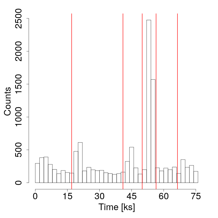
Figure 1: The light curve of the combined UV Cet system, with a time bin size of $\approx$ 1500 s. Our data-driven procedure is deployed to identify the five break points denoted by the red vertical bars.

In order to account for temporal changes, we split the data into possibly irregular bins that capture the variations in the observed light curve of the system. There is a trade-off here between the fineness with which one wants the variability to be modeled on the one hand, and the data size that allows useful uncertainty intervals on the fitted parameters, the total number of parameters, and the running time. The dimension of the parameter space scales linearly with the number of time segments; for the sake of parsimony as well as to avoid unnecessarily complex calculations, a small number of segments is preferred. The temporal segmentation model is not designed to capture subtle variations directly, but rather aims to improve disambiguation between overlapping photon events.

We thus allow the number of breakpoints to be set on a case by case basis, and choose as the breakpoints those times which show the largest changes in counts in adjacent bins. Given the user-specified number of breakpoints, we develop a simple data-driven procedure to identify the locations that best isolate transient variations and flares in the light curves. The procedure first divides the event-arrival times into a high-resolution histogram and then identifies the adjacent bins with the largest differences in intensity. The breakpoints are set to separate these bins; see Figure 1 for an illustration of this method in the case of the UV Cet light curve with the number of breakpoints preset to five. Finally, the algorithm merges all of the histogram bins between the selected breakpoints to obtain the target number of time intervals. Full details appear in the form of pseudo-code in Appendix B; computer code is included in the eBASCS software package available on the CHASC GitHub software library.

2.7 Statistical Models and Likelihoods

Here we combine the spatial, spectral, and temporal models into the overall models that we use and compare in this article. We refer to the model that only incorporates spatial data, $\{(x_{i},y_{i})\}_{i=1}^{n}$, as the baseline or spatial model. Its parameters are denoted by $\Theta=\{\mu_{j}\}_{j=1}^{S}$, and the corresponding likelihood is:

$$L^{{\tt spatial}{}}(\Theta,s)\propto\prod_{i=1}^{n}\prod_{j=1}^{S}w_{j}f_{\mu_{j}}(x_{i},y_{i}).$$ (12)

BASCS (Jones et al., 2015) models observed event spatial and energy data: $\{(x_{i},y_{i},E_{i})\}_{i=1}^{n}$. The parameters for this model are denoted $\Theta=\{\mu_{j},\theta_{j}\}_{j=1}^{S}$, and the corresponding likelihood is:

$$L^{{\tt BASCS}{}}(\Theta,s)\propto\prod_{i=1}^{n}\prod_{j=1}^{S}w_{j}f_{\mu_{j}}(x_{i},y_{i})g_{\theta_{j}}(E_{i}).$$ (13)

The proposed method, eBASCS, models observed event spatial, spectral and temporal data: $\mathbf{x}=\{(x_{i},y_{i},t_{i},E_{i})\}_{i=1}^{n}$. The parameters for this model are denoted $\Theta=\{\mu_{j},\theta_{j},\lambda_{j}\}_{j=1}^{S}$, and the corresponding likelihood is:

$$L^{{\tt eBASCS}{}}(\Theta,s)\propto\prod_{i=1}^{n}\prod_{j=1}^{S}\prod_{k=1}^{K}w_{j}\lambda_{jk}f_{\mu_{j}}(x_{i},y_{i})g_{\theta_{j}}(E_{i}).$$ (14)

Some X-ray detectors do not record the energy of the observed events with useful accuracy , e.g., the Chandra/HRC-S detector used to record the UV Cet observation analysed in Section 5. In such cases, it is useful to consider a spatio-temporal model that only includes the spatial and temporal components. We refer to this model as the space+time model. The parameter for this model is $\Theta=\{\mu_{j},\lambda_{j}\}_{j=1}^{S}$, which yields the likelihood:

$$L^{{\tt space+time}{}}(\Theta,s)\propto\prod_{i=1}^{n}\prod_{j=1}^{S}\prod_{k=1}^{K}w_{j}\lambda_{jk}f_{\mu_{j}}(x_{i},y_{i}).$$ (15)

3 Bayesian Inference and Statistical Computation

3.1 Inferential approach

We adopt a Bayesian statistical approach. This allows us to quantify uncertainty in the model parameters via their joint (posterior) distribution given the observed data. From this we can compute point estimates and error bars, if required. The Bayesian paradigm also allows us to incorporate existing scientific knowledge about the likely values of the parameters into the model via their prior distributions. Once the prior distributions are specified and the data is observed (and integrated into the model via the likelihood), Bayes’ Theorem gives the expression for the posterior distribution of the parameters, i.e., the updated beliefs about the model parameters after observing the data:

$$p(\Theta,s|\mathbf{x})=\frac{p(\mathbf{x}|\Theta,s)p(\Theta,s)}{p(\mathbf{x})},$$ (16)

where $p(\mathbf{x}|\Theta,s)\equiv L(\Theta,s)$ is the likelihood of the data under the chosen model, $p(\Theta,s)$ is the prior distribution of the parameters, and $p(\mathbf{x})$ is the marginal distribution of the data. While $p(\mathbf{x})$ is sometimes used for model selection, for the purposes of Equation 16, it can be viewed as a normalizing constant and need not be computed. Our choices of prior distributions are discussed in Section 3.2.

3.2 Specifying prior distributions

Our general approach is to specify uninformative and computationally practical prior distributions. In our applications, we usually observe a large enough data set to mitigate the effect of the prior distributions on posterior inference. However, any information about likely parameter values can and should be encoded into the prior distributions.

Following Jones et al. (2015), we specify uniform (across the image) priors on the source locations:

$$\mu_{j}\sim\text{Uniform}$$ (17)

for $j=1,\dots,S$ , but one could also specify a distribution centered at a likely value $\mu_{j0}$ for $\mu_{j}$. The prior distributions for the other parameters are those given in Jones et al. (2015). The parameters that are probability vectors, $\mathbf{w}$ and $\lambda$, and govern the Multinomial splitting of events among sources and time bins, respectively, are given Dirichlet prior distributions. Picking conjugate prior distributions (like Dirichlet priors for Multinomial likelihoods) is computationally convenient, and allows for more transparent interpretations of posterior inferences (Gelman et al., 2013). Hence:

$$\mathbf{w}\sim\text{Dirichlet}(\eta,\dots,\eta),$$

$$\lambda\sim\text{Dirichlet}(\zeta,\dots,\zeta).$$ (18)

Following Jones et al. (2015), the above hyperparameters are set at $\eta=\zeta=1$, so that the prior distributions correspond to as much information as a single event added to each source (or each time bin for $\lambda$).

For a spectral model defined as a single Gamma distribution, we use the prior distributions, $\alpha_{j}\sim\text{Gamma}(2,0.5)$ and $\gamma_{j}\sim\text{Uniform}(E_{min},E_{max})$. If a mixture of two Gamma distributions is used for the spectral model, a reasonable choice for the mixture weight parameter is a Beta(2,2) distribution (assuming a 2-components mixture), again following Jones et al. (2015).

3.3 Statistical Computation

In order to derive useful summaries of the posterior distribution of the model parameters, we generate a Monte Carlo sample of parameter values from the posterior. Indeed, for an unknown model parameter $\mu$ with marginal posterior distribution $p(\mu|\mathbf{x})$, a sample $\{\mu^{(1)},\dots,\mu^{(N)}\}$ of $N$ draws from the posterior allows us to compute point estimates and error bars for $\mu$, e.g., via the mean and standard deviation of the sample if the posterior is roughly Gaussian (e.g., Stenning & van Dyk, 2021), or more generally via quantiles of the sample.

We use Markov Chain Monte Carlo (MCMC) to obtain a sample of $(\Theta,s)$ from its joint posterior distribution, $p(\Theta,s|\mathbf{x})$. A Markov chain is a set of sequentially sampled random variables, $(\Theta,s)^{(t)}$, for $t=1,2,\ldots$, such that each $(\Theta,s)^{(t)}$, depends on the history of the chain only through the most recent iterate, $(\Theta,s)^{(t-1)}$. MCMC methods are a class of iterative algorithms that produce a Markov chain with stationary distribution equal to the target Bayesian posterior distribution. If run for a sufficient number of iterations, the marginal distribution of each of the (correlated) iterates of the chain approaches the target posterior distribution. Thus, if the sample that is comprised of the MCMC iterations before the chain reaches approximate convergence (i.e., the burn-in iterations) is discarded, the remaining sample (i.e., the main run) can be treated as a correlated sample from the target posterior distribution. In our simulations, we typically discard the first half of the chain as burn-in.

Positively correlated samples carry less information than independent samples of the same size, and thus yield estimates of posterior quantities with higher Monte Carlo error. The Effective Sample Size (ESS) approximates how large of an independent sample would contain the same level of information as our correlated MCMC sample (e.g., Stenning & van Dyk, 2021). In our numerical studies and examples, we choose the number of main-run iteration to obtain an ESS between 1000 and 2000. Generally, this requires a total run of about 40,000 iterations. (We discard the first half of each chain as burn-in and thin the remainder, saving only every tenth iterate, to reduce memory requirements.) We also monitor convergence of the chains through visual diagnostics such as trace plots and auto-correlation plots. For a more detailed discussion of practical considerations involved with MCMC, the reader is referred to Gelman et al. (2013) or, for a more astronomy-oriented account, to Stenning & van Dyk (2021). We develop both R code for MCMC methods based on the Metropolis algorithm (Metropolis et al., 1953) and STAN code which implements Hamiltonian Monte Carlo (Duane et al. (1987), Neal (2011)).

Naturally, our methodology has certain limitations. Here we detail two and propose solutions. Finite mixture models, such as the one we use with eBASCS, produce multi-modal posterior distributions, which are notoriously difficult to explore via MCMC and thus require special care. The most obvious and important issue is the possibility that the algorithm becomes "stuck" in one mode, and thus fails to explore the full posterior distribution. To give a more detailed example, consider a binary star system, with unknown location parameters $\mu_{1}$ and $\mu_{2}$. If the sources are well separated, it might happen that the MCMC samples of both $\mu_{1}$ and $\mu_{2}$ converge to the location of source 1, see Figure 2. This worry can be addressed by choosing starting values for $\mu_{1}$ and $\mu_{2}$ at random locations along the edges of the image close to the respective sources. Another option, that we recommend, is to initialize the location parameter values at the approximate location of the modes of the spatial image of observed event locations, e.g., found by applying Kernel Density Estimation (KDE) to the raw images. We have not found it necessary to implement sophisticated multi-modal sampling techniques (e.g., parallel tempering (Geyer, 1991) or evolutionary Monte Carlo (Liang & Wong, 2000)) since the failure mode has been obvious and the remedies easily implemented.

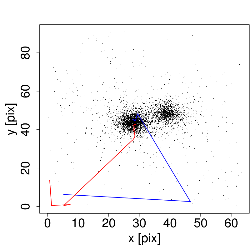
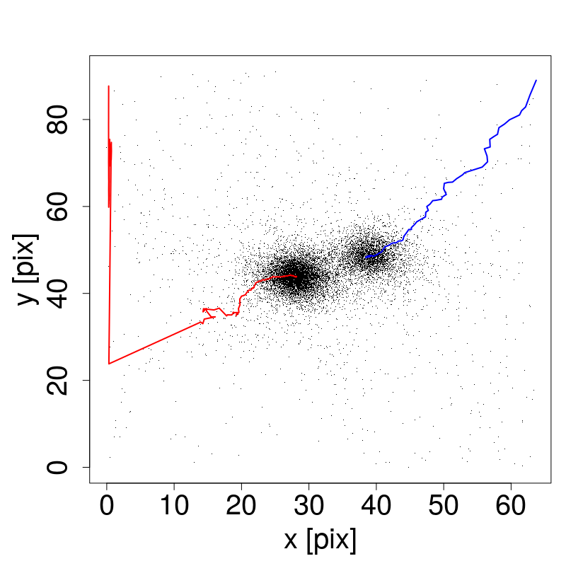
Figure 2: Examples of the convergence the location parameters’ MCMC iterates. Both panels show the recorded spatial coordinates of the UV Ceti (Gliese 65) binary system, analyzed in Section 5. Left Panel: With poor choice of initialization, both fitted location parameters, $\mu_{1}$ (red) and $\mu_{2}$ (blue), converge to the location of source to the left of the image. Right Panel: When better initialized, they converge to their respective true locations.

Another possible concern is thatresult in computational inefficiency. For instance, the source locations $\mu_{1}$ and $\mu_{2}$ can only take values within the boundaries of the image, and the spectral parameters must be positive. Using a standard Metropolis proposal distribution for these parameters, such as a normal distribution centered on the current value, leads to severe inefficiency in the algorithm since proposed values outside of the parameter’s support must be rejected, which induces sub-optimality in the Metropolis acceptance rate. To remedy this, we log-transform the parameters to eliminate the constraints on their support. This allows us to efficiently implement a normal proposal distribution (on the logarithmic scale).

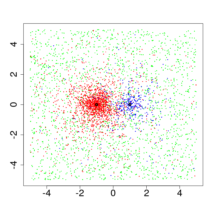
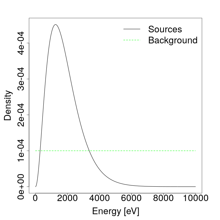
Figure 3: Illustrative simulation design, with parameters $r=5$, $d=2$, $b=1$. Left Panel: Scatter plot of simulated event locations for the bright source (red), the dim source (blue) and the background (green). True source locations are marked by the black circles. Middle Panel: Spectra used to simulate the source and background event energies. Right Panel: Observed light curves for the sources and background.

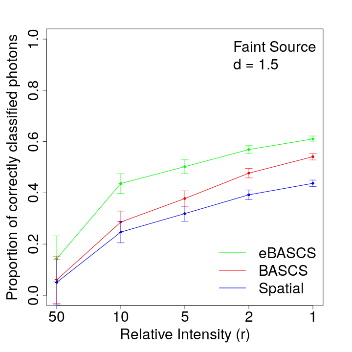
Figure 4: Average proportion of events originating from the faint source that were correctly classified by the eBASCS (green), BASCS (red) and spatial (blue) algorithms, for simulation settings $(d=1.5,r\in\{1,2,5,10,50\})$, averaged over the replicate data sets. This plot is replicated for the other simulation studies in Appendix C.

4 Simulation Studies

In this section, we evaluate the benefit of incorporating temporal data, by comparing the performance of eBASCS with the BASCS and spatial algorithms on simulated data sets. Our simulations are parametrized in terms of a range of background intensities, spatial source separations, and relative source intensities. They are organized into two simulation studies that differ in terms of the strength of the background. Simulation I, described in Section 4.2, constructs a challenging scenario where one source is weak compared to the background contamination. Simulation II, described in Section 4.3, considers a more realistic situation where the background is weaker than the sources, in order to mimic the level of background encountered with modern high-resolution X-ray telescopes like Chandra. Section 4.1 sets up the general simulation design, which applies to both Simulations I and II.

4.1 Simulation Design

Our simulation design involves two astronomical objects, one brighter than the other, emitting photons in an image of 10 by 10 spatial units. The first simulation setting is the distance between the two sources, denoted as $d$, and we consider the set of values $d\in\{0.5,1,1.5,2\}$. In each simulation, the number of events originating from the background and sources are drawn from Poisson distributions with respective means $m_{0}$, $m_{1}$ and $m_{2}$. The brighter source has $m_{1}=2000$, while the fainter source’s intensity is defined as $m_{2}=m_{1}/r$, where $r$ denotes the relative intensity of the two sources and is the second simulation setting. We consider the set of values $r\in\{1,2,5,10,50\}$. The strength of the simulated background $m_{0}$ differs between Simulation I and II, see Sections 4.2 and 4.3 for details.

We also generate spectral data for the source and background events. Since the focus of Simulations I and II is to investigate how much we can improve the fitted parameters and event allocations by incorporating temporal data, we use a common spectra for both sources (rather than different spectra between the sources or between the time bins). Specifically, the two sources have a common spectra generated from a Gamma distribution with shape parameter $\alpha=3.18$ and mean $\gamma=1832$; these particular parameter values follow Jones et al. (2015). The background spectra is generated from a Uniform distribution.

To simulate the temporal data (in the form of arrival times for the events), a 60ks observation period is defined and split into four equally sized time bins. Events are allocated to each time bin according to a Multinomial distribution with parameters $(\lambda_{1},\lambda_{2},\lambda_{3},\lambda_{4})=(0.05,0.15,0.3,0.5)$ for the bright source, and $(\lambda_{1},\lambda_{2},\lambda_{3},\lambda_{4})=(0.5,0.3,0.15,0.05)$ for the faint source. This means that the bright source gets brighter over time, and that the faint source dims over the observation period (see right panel of Figure 3). Background events are spread uniformly among the time bins. The number of parameters to be fitted for eBASCS grows linearly with the number of time bins. Simulating data and fitting the model with four time bins is a reasonable option to both generate enough discriminatory temporal information and moderate the required computational complexity.

In Simulation I, replicate data sets were generated under 20 different settings, crossing $r\in\{1,2,5,10,50\}$ and $d\in\{0.5,1,1.5,2\}$. In Simulation II, 5 different settings were considered, crossing $r\in\{1,2,5,10,50\}$ and $d=1$. Evaluating the performance of eBASCS in this way ensures its consistency with the expected behaviour of a disentangling model in the physical environments represented by the datasets. In particular, the two sources are expected to be increasingly distinguishable as their spatial separation, $d$, grows. Similarly, as $r$ gets large the model is expected to easily detect the brighter source but detection of the dimmer source may remain difficult. Fifty replicate data sets were generated for each of the 20 settings in Simulation I, and each of eBASCS, BASCS and spatial were run on each replicate. For Simulation II, fifty replicate data sets were generated for each of the 5 settings, and each of eBASCS, space+time, BASCS and spatial were run on each replicate.

4.2 Simulation I: High Background

In Simulation I, the strength of the simulated background $m_{0}$ is defined as a function of the faint source region and intensity. Specifically, we set $m_{0}$ so that the expected number of background and faint source counts is equal in the faint source region (defined as the area where the PSF is greater than 3$\%$ of its maximum). Mathematically, we let $q$ be the probability that a event from the faint source falls within this source region and set $m_{0}=qm_{2}$. This results in very intense background that strongly overwhelms the fainter source, allowing us to investigate to what extent eBASCS outperforms BASCS and spatial in an extremely noisy environment.

At each MCMC iteration, updated allocations of the events to sources or background are drawn from a Multinomial distribution with probabilities given by the posterior distribution for the variable $s$, computed with the latest sampled parameter values. From these allocations, two metrics are computed to measure the classification performance of eBASCS. Specifically, we report

Allocation Recovery:

The proportion of events originating from a source that were indeed allocated to that source.

Allocation Accuracy:

The proportion of events allocated to a source that actually originate from this source.

All proportions are averaged over both MCMC iterations and replicate data sets. Averaging over the replicate data sets reduces sampling variability, which can be substantial in low-count simulation settings (between 2000 and 4000 counts with $r\in\{50,10,5\}$). Relying on a single replicate data set might not accurately reflect the relative performance of the methods. Tables 2 and 3 report the two metrics, respectively, averaging over the 20 simulation settings. Appendices D.1 and D.2 report complete results for each simulation setting separately.

As expected, on average eBASCS performs substantially better at disentangling overlapping sources than either BASCS or spatial. This provides strong evidence of the ability of the proposed method to leverage the temporal information to extract discriminatory features. Tables 2 and 3 show that all models are less able to properly allocating events to the faint source than to the bright source. This is a direct consequence of the simulation design. Under the simulation settings where $r$ is large ($r\geq 5$), the faint source is completely overwhelmed by the strong background. For example, with a relative intensity of $r=5$, the expected number of faint source and background events are $m_{2}=400$ and $m_{0}\approx 1920$, respectively, while the expected number of bright source events is $m_{1}=2000$.

True Source	eBASCS	BASCS	spatial
Bright Source	0.771	0.723	0.651
Faint Source	0.420	0.307	0.252
Background	0.831	0.822	0.722

Table 2: Allocation recovery for each source by eBASCS, BASCS, and spatial. The proportions are averaged over MCMC iterates, replicate data sets and simulation settings. A breakdown according to simulation settings appears in Appendix D.1.

Allocated Source	eBASCS	BASCS	spatial
Bright Source	0.798	0.744	0.686
Faint Source	0.424	0.310	0.264
Background	0.803	0.794	0.671

Table 3: As in Table 2, for allocation accuracy. A breakdown according to simulation settings appears in Appendix D.2

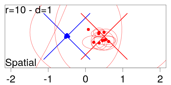
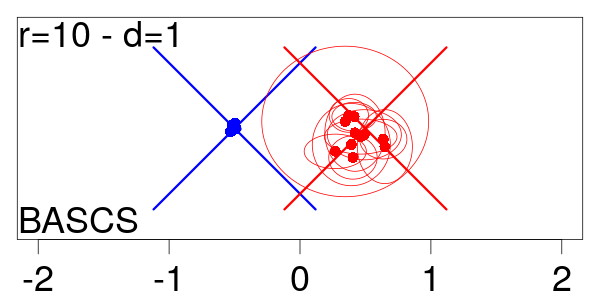
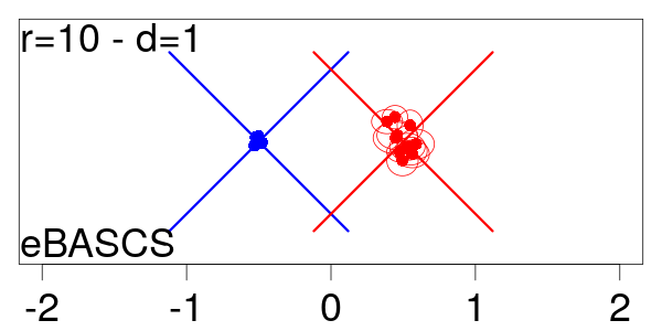
Figure 5: Posterior means and standard deviations of the source locations for 10 replicate data sets generated under the simulation setting with $r=10$ and $d=1$ and fit with the spatial (Left Panel), BASCS (Middle Panel) and eBASCS (Right Panel) algorithms. The points and ellipses represent the posterior means and standard deviations for each of the ten replicates; those for the bright source are plotted in blue and those for the faint source in red. Crosses indicate the true location of the sources. eBASCS is able to locate the faint source much more consistently (the posterior means of the location are closer to the true value) and confidently (the posterior standard deviations are much smaller) than the other methods.

Figure 4 shows that classification performance for the faint source improves as its relative intensity grows (i.e., as $r$ decreases). In the simulation setting with $r=1$ and $d=0.5$, eBASCS had an allocation recovery of $57.1\%$ of the bright source events and $56.4\%$ of faint source events (see Table 9 in Appendix D.1). That is, in a setting where the sources are extremely close, have the same spectra and relative intensity, and are immersed in an exceedingly strong background, eBASCS still correctly classifies more than half of events from the sources. This is a substantial improvement over BASCS, which had an allocation recovery of only $42.8\%$ of bright source events and $42.2\%$ of faint source events in the same simulation setting (see Tables 9 and 15 in Appendix D.1).

The biggest improvement of eBASCS over the other algorithms is its ability to distinguish faint sources from background, particularly when the relative intensities of the bright and faint sources are extreme. In such a case, BASCS and spatial sometimes mistake the faint source for a random cluster of events from either the brighter source or the background. In the middle panel of Figure 11 in Appendix C, for the simulation setting $r=10$ the allocation recovery of faint source events by BASCS and spatial is close to 0, which indicates that these algorithms cannot separate the faint source from the bright source or the background. eBASCS, however, is able to better distinguish the faint source and has an allocation recovery of around 20$\%$. Incorporating the temporal data allows eBASCS to partially solve this problem, and to provide more precise and confident event allocations.

In addition to probabilistically attributing events to sources, eBASCS provides estimates and error bars for the model parameters. Figures 16 and 16 (in Appendix E) illustrate the statistical properties of the estimates by plotting the posterior means of the two source locations for all 50 replicate data sets under each of the 20 simulation setting. Crosses indicate the true source locations. The variance among replicate data sets of the posterior mean of the bright source’s location increases as $r$ decreases, i.e., as the faint source becomes relatively brighter and the background intensifies compared to both sources. (Recall that the background intensity is tied to the faint source intensity.) The location of the faint source, however, is estimated more accurately as it grows brighter (i.e., as $r$ decreases). Particularly, when it is bright enough for the algorithms to detect an energy signature that is distinguishable from the background spectrum.

The eBASCS algorithm yields fits that are at least as accurate as BASCS. Even when the sources are closely located (i.e., $d=0.5$), the eBASCS-fitted posterior means of the source locations concentrate more closely around the true locations than those provided by BASCS. With $d=0.5$, the separation between sources and background relies heavily on the energy model and the spatial algorithm does not perform as well as either BASCS or eBASCS.

The specific simulation setting with $r=10$ and $d=1$ is illustrated in Figure 5 and shows that eBASCS is not only able to locate the sources more accurately, as its posterior means cluster more closer to the true location, but also more confidently, since the eBASCS standard deviations (circling the posterior means in Figure 5) are much smaller than those of BASCS and spatial. This also holds for the other model parameters, see Appendix F for a full comparison of the parameter estimates.

To investigate the number of counts eBASCS requires to produce meaningful results, we repeated the simulation setting illustrated in Figure 5 ($r=10$, $d=1$) but with $m_{1}=\{800,600,400\}$; recall that $m_{1}$ is the expected count for the brighter source and was originally set to $m_{1}=2000$ in Simulation I. Even with $m_{1}=400$, corresponding to about 100 counts per time bin, the posterior means of the source locations cluster closely around their true values.

4.3 Simulation II: Low Background

The background intensities in Simulation I are by design the same as the intensity of the faint source. The background in modern high-resolution X-ray telescopes similar to Chandra, however, is typically weaker than this. Simulation II assesses how eBASCS performs in a more realistic and plausible noise environment. It considers scenarios where the total background count is drawn from a Poisson distribution with mean $m_{0}=100$.

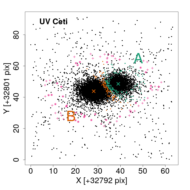
Figure 6: Sky pixel locations of photon events disputed by the spatial and space+time algorithms for UV Cet. Events coloured in black were allocated to the same source by both algorithms. Events coloured in orange were allocated to UV Cet B by the spatial algorithm and UV Cet A by the space+time algorithm. Events coloured in green are the opposite, i.e., allocated to UV Cet A by spatial but to UV Cet B by space+time. Disputed background events are marked as magenta symbols (“+” denoting those reallocated to a source, and “*” are those reallocated to the background by space+time).

The allocation recovery and allocation accuracy for each algorithm and setting in Simulation II are reported in Appendix G. Tables 4 and 5 average these metrics across relative source intensities, $r$, to summarize the overall performance of the algorithms in Simulation II. The fact that the space+time algorithm outperforms BASCS for both sources is not unexpected. Because both sources are simulated with the same spectrum, the spectral data do not help distinguish between the two sources (but do help to separate out background events). Temporal data, however, do help to distinguish the two sources. Since background counts are low in Simulation II, the added benefit of spectral data is small compared to that of temporal data, as illustrated by the almost imperceptible improvement of BASCS over the spatial algorithm.

True Source	eBASCS	BASCS	space+time	spatial
Bright Source	0.869	0.804	0.841	0.810
Faint Source	0.495	0.346	0.499	0.334
Background	0.580	0.570	0.315	0.200

Table 4: Allocation recovery. As in Table 2, for Simulation II by eBASCS, BASCS, space+time and spatial. A breakdown according to simulation settings appears in Appendix G.1.

Allocated Source	eBASCS	BASCS	space+time	spatial
Bright Source	0.878	0.820	0.870	0.780
Faint Source	0.484	0.334	0.338	0.482
Background	0.523	0.515	0.305	0.221

Table 5: Allocation accuracy. As in Table 4, for allocation accuracy. A breakdown according to simulation settings appears in Appendix G.2.

5 Application I: UV Ceti

5.1 Data and Models

UV Ceti (Gliese 65) is an M dwarf hierarchical binary system. Both the main components of the binary, UV Cet A and UV Cet B are flare stars that undergo unpredictable and dramatic changes in their brightness over short timescales. The UV Cet system was observed with Chandra on 2001 Nov 26 (ObsID 1880) with the LETGS+HRC-S configuration. The spatial resolution of Chandra is sufficient to visually distinguish the two components, which are separated by a distance of 1.4 arcsec (UV Cet B is itself a binary (Benz et al., 1998), but with a separation of $\sim$1 mas, it is not resolvable by Chandra). These data have been previously analyzed to separate the two components (see Audard et al., 2003) using small extraction radii to limit contamination of one source due to the other. However, UV Cet B undergoes a large flare during the observation, and its effect is also visible in the light curve of UV Cet A (Audard et al., 2003, see Fig. 2). This source is thus a natural test case for the application of the eBASCS algorithm. Since the HRC-S has no spectral discrimination, applying BASCS to the $0^{\rm th}$-order data to separate the events from the two sources will not yield any improvements over the spatial algorithm. We demonstrate below that the space+time algorithm does lead to a significantly better allocation of events.

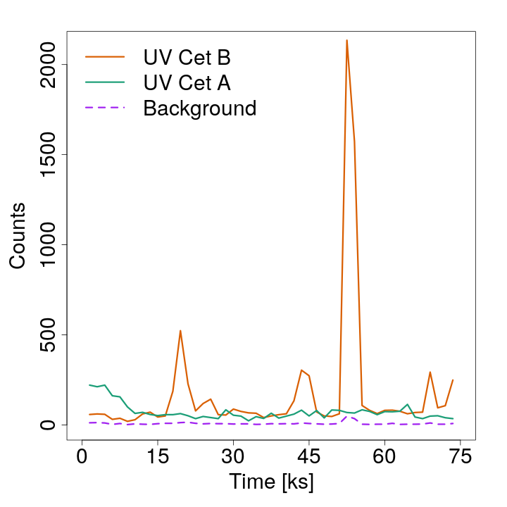
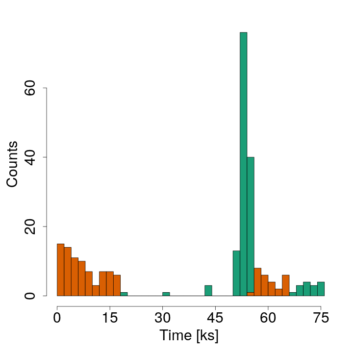
Figure 7: Left Panel: Light curves for UV Cet A, UV Cet B and the background obtained from an single Monte Carlo iteration of the space+time algorithm. There is moderate contamination from the UV Cet B’s flare (at around 53ks) on the background. This contamination is less severe than with the spatial  algorithm; space+time allocated 84 events to the background at the time of the UV Cet B flare, while spatial allocated 106 events to the background. (Such contamination is also a consequence of the approximate nature of our PSF model.) Right Panel: Arrival times of events disputed by the spatial and space+time algorithms. The orange bars indicate events that are moved from UV Cet B to UV Cet A, and green bars indicate events that are moved from UV Cet A to UV Cet B by the space+time model. Events allocated to the same source by both algorithms are not included in the plot. Notice that space+time is successful in identifying the contamination in UV Cet A due to the large flare of UV Cet B and allocating those events to UV Cet B.

We selected the time bins for UV Cet using the procedure detailed in Section 2.6. We chose 6 time bins which renders a temporal model that is flexible enough to capture the source flare at $\approx$54 ks after the start of observation (see Figure 1) while maintaining a reasonable number of model parameters to be fit with the space+time algorithm (25 parameters i.e., 4 location, 3 relative intensity and 18 time intensity parameters).

5.2 Results

To measure the difference of the space+time model over the spatial model, we carry out a disputed event analysis. This consists of comparing the allocations of the events in the two algorithms and studying the characteristics of disputed events to highlight the benefits of incorporating temporal information. For each event $i$, the disentangling models output the posterior distribution of $s_{i}$, the latent variable that encodes its origin. For each model, we set the allocation of event $i$ to the source it has the highest probability of originating from, i.e., event $i$ is allocated to the bright source if $p(s_{i}=\text{bright})=\max\{p(s_{i}=\text{bright}),p(s_{i}=\text{faint}),p(s_{i}=\text{background})\}$.

Figure 6 shows that, as expected, most disputed events are located in the zone where the source wings overlap, or in other words where events are roughly equidistant from both cores. In this case, the space+time algorithm performs a more careful analysis of events in the overlap between the sources, i.e., in locations where it is most difficult to separate the sources based on spatial data alone.

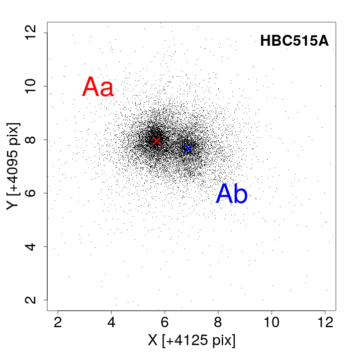
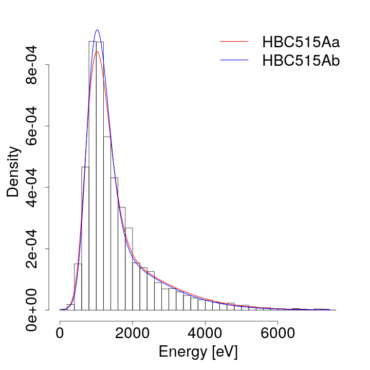
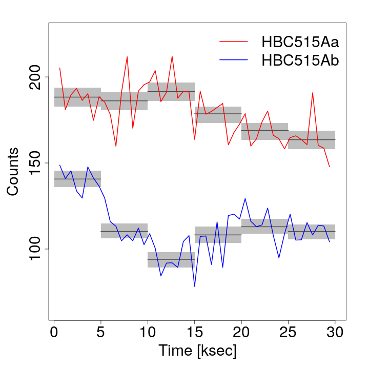
Figure 8: ${\it Chandra}$ ACIS-S observation of the binary system HBC 515 A. Left Panel: Scatter plot of recorded event locations with the posterior means of the locations of HBC 515 Aa and HBC 515 Ab computed with BASCS plotted as red and blue crosses, respectively. Middle Panel: Histogram of spectral data with source spectra superimposed (using the posterior mean of the spectral parameters fitted with BASCS) . Right Panel: Light curves for the two separated components of HBC 515 A obtained by allocations made by eBASCS, superimposed with the eBASCS-fitted light curves (grey). The red and blue curves denote the average of the allocated light curves over 500 iterations of eBASCS, the dark gray horizontal lines denote the posterior mean of the temporal parameters fitted by eBASCS, and the light grey regions denote the intervals between the 16$\%$ and 84$\%$ posterior quantiles (see Table 7).

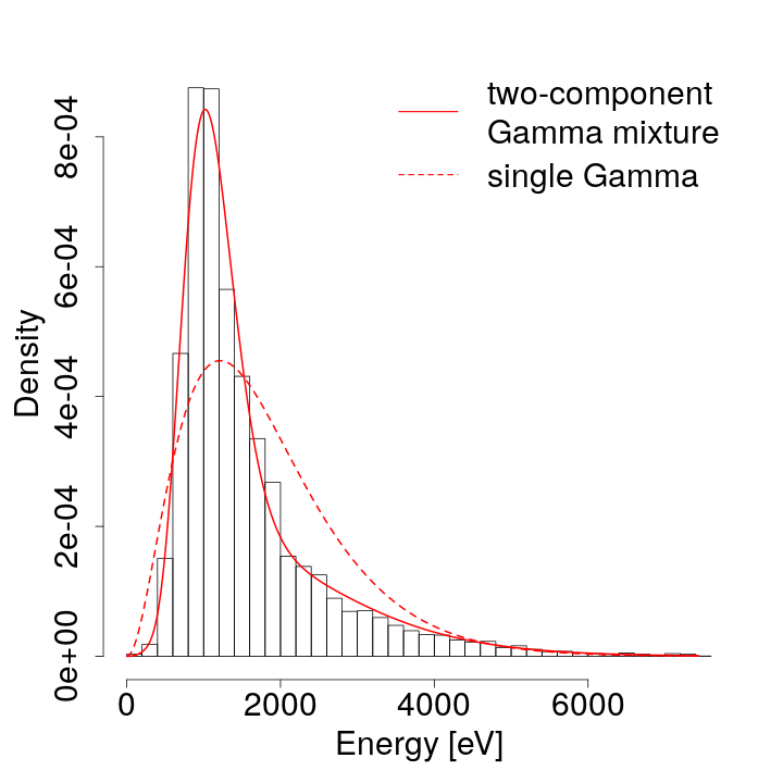
Figure 9: Fitting a single-Gamma distribution and a two-component mixture of Gammas distributions to the spectral data for HBC 515 Aa. The histogram shows the observed spectrum of the HBC 515 A system (i.e, all sources combined). Note that the middle panel of Figure 8 indicates that HBC 515 Aa and HBC 515 Ab have very similar spectra. The solid line is the fitted two-component mixture of Gammas and the dashed line is fitted the single Gamma model.

The recorded locations of the disputed events allocated to UV Cet A by spatial, circling around the source’s core, indicate that these events were assigned to UV Cet B by space+time on the basis on temporal information. Indeed, as illustrated in the right panel Figure 7, these events were all detected at the time coincident with an observed flare attributed to UV Cet B. The right panel shows that this contamination of the flare of UV Cet B on UV Cet A is completely removed by eBASCS, as the lightcurve of UV Cet A (as allocated by eBASCS) does not exhibit a spike in its intensity at the time of the flare. Figure 7 also shows that the contamination of UV Cet A on UV Cet B at early times (between 0ks and approximately 15ks), i.e., when UV Cet A has higher intensity, is removed by eBASCS.

	UV Cet B	UV Cet A	Background
UV Cet B	8388	149	28
UV Cet A	107	3560	19
Background	23	5	381

Table 6: Disagreement matrix between the allocations made by the space+time and spatial algorithms. Columns correspond to the allocations made by spatial and rows correspond to allocations made by space+time. For example, 149 events that were attributed to UV Cet A by spatial were instead allocated to UV Cet B by space+time.

Table 6 reports the disagreement matrix (i.e., the number of events allocated to each source by both algorithms). Adding temporal data changed the allocation of 331 (out of 12,660) events, 149 of which correspond to the contamination of UV Cet B’s flare on UV Cet A, and 107 of which correspond to the contamination of UV Cet A on UV Cet B in the early stages of the observation period. Removing these contaminations would not have been possible without modelling the temporal information, and clearly shows the improvement of space+time over the spatial algorithm.

6 Application II: HBC 515 A

6.1 Data and Models

HBC 515 A is a component of the well-separated weak-lined T Tauri multi-component system HBC 515 (Reipurth et al., 2010). HBC 515 A is a binary, composed of two variable stars, HBC 515 Aa and HBC 515 Ab, separated by a distance of approximately 0.5 arcsec. The system was observed with Chandra/ACIS-S on 2011 January 8 (ObsID 12383). The overlap of the PSFs of the two components is significantly larger than UV Cet, and separating them through non-overlapping extraction regions would lead to a significant loss in the number of counts available for follow-up analyses. Such an analysis was performed by Principe et al. (2017), who used a complex set of regions covering the cores and the diametrically-opposed crescent-shaped wings to extract the events and conduct spectral and temporal analyses. They found that the spectra accumulated over the duration of the observation were similar, and that there was no evidence for temporal variability. In the following, we demonstrate that even in this challenging dataset, eBASCS is able to recover small temporal changes to both the intensities and spectra of the two components. Not only do the data show that the spectra of both stars vary stochastically over timescales of a few ks, but that at different times different components are observed to be spectrally harder.

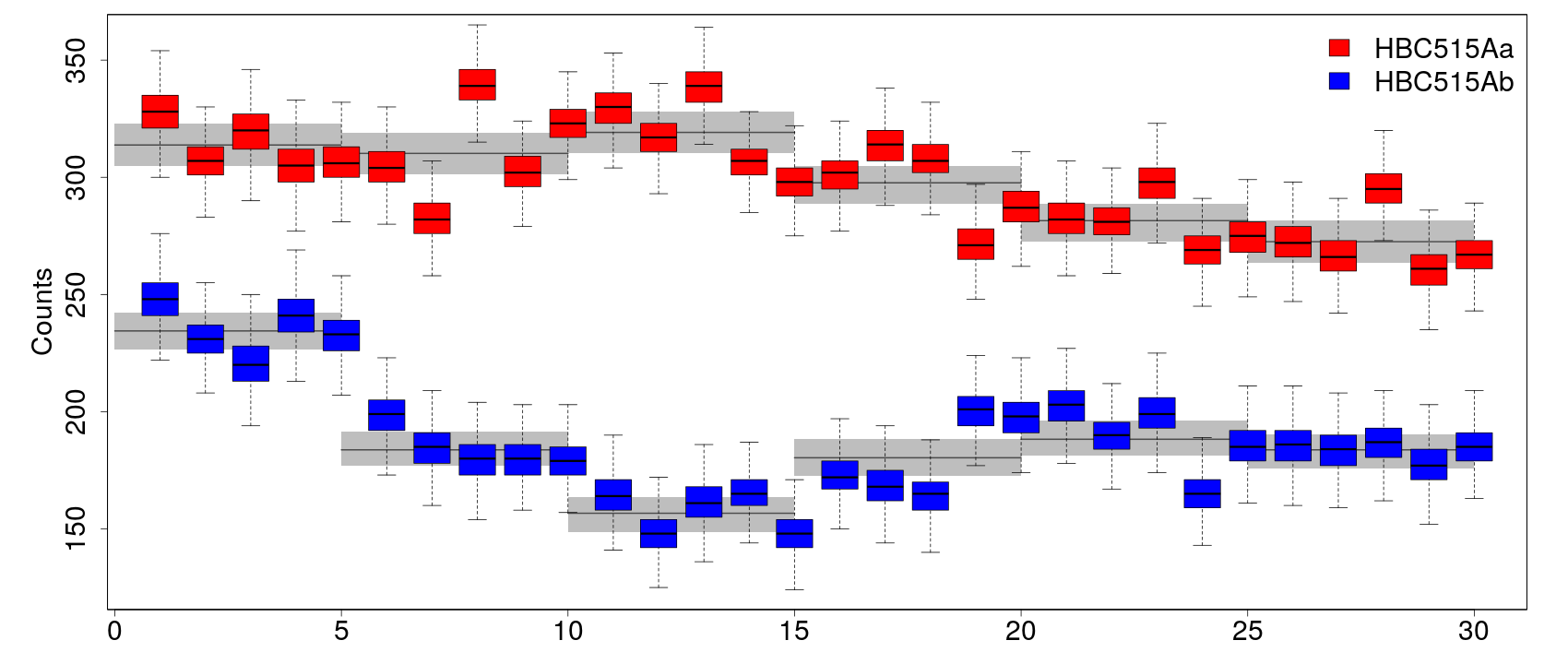
Figure 10: Spectral and intensity variability in the components of HBC 515 A, constructed using event allocations from 500 iterations of eBASCS. Top and Bottom Panels: Spectral hardness in the Soft ($S$:0.3-0.9 keV), Medium ($M$:0.9-2 keV), and Hard ($H$:2-8 keV) bands (Top: C${}_{SM}=\log\frac{S}{M}$; Bottom: C${}_{MH}=\log\frac{M}{H}$) are shown for events grouped into 1 ks bins for both the HBC 515 Aa (red) and HBC 515 Bb (blue) components. The posterior distributions of spectral color are shown oriented vertically for each time bin. These so-called violin plots are normalized so that the modes have the same horizontal displacements; thicker part of each color segment denote a higher posterior probability of the ordinate in a given time bin. In both panels, the left halves of the shapes represent HBC 515 Aa, and the right halves represent HBC 515 Ab in order to facilitate comparisons. Counts for the individual violin plots for HBC 515Aa vary from 49-76 (Soft), 146-196 (Medium), and 43-85 (Hard); counts for HBC 515Ab vary from 28-50 (Soft), 84-150 (Medium), and 22-55 (Hard). Middle Panel: Intensity variations in the combined broad ($B=S+M+H$:0.3-8 keV) passband are shown for the same time binning and demonstrate the evolution of the brightness of each component. The fitted intensities $\lambda_{i,j}$ in each time segment (see Table 37) are shown as grey bands. Overall the panels illustrate several instances of spectral changes, e.g., HBC 515 Aa is spectrally harder at the beginning of the observation (see C_MH), and is spectrally softer near the 25 ks mark (see C_SM); HBC 515 Ab shows increasing spectral hardening as it recovers from its minimum brightness.

The HBC 515 A dataset is comprised of 14601 events recorded over 28.76 ks. We first extract the events over a range of sky pixels large enough to include both components of the binary, but exclude other components of the system (see Figure 8).

Since the ACIS detectors do allow for event energy discrimination, we apply the eBASCS algorithm to the HBC 515 A data, allowing us to characterize the time variability of both HBC 515 Aa and HBC 515 Ab. We use eBASCS with the number of sources fixed at $S=2$, and for simplicity adopt the King profile density (Appendix A) as the PSF model. We use six equally-spaced time bins to model temporal variations, as this choice presents a practical trade off between preserving the flexibility in modeling while limiting the size of the parameter space. We model the counts spectra in three different ways: first, using the single-Gamma distribution (Equation 6) for each source ; second, using the two-component mixture of Gamma distributions (Equation 2.4) for each source; and third, using a two component mixture at each time bin for each source (Equation 11). As discussed by Jones et al. (2015), a crude spectral model that roughly tracks the shape of the astrophysical model spectrum weighted by the effective area has sufficient power to distinguish spectral variations between the sources. We use a uniform spectral model for the background.

6.2 Results

The two-component mixture of Gamma distributions (Equation 2.4) fits the observed counts spectra better than the single-Gamma distribution (see Figure 9). Unfortunately, the very few counts in each time bin per source leads to large uncertainties in the parameter estimates under the spectral model that incorporates a two component mixture at each time bin. Moreover, the spectra of the sources do not appear to be variable enough to justify the complexity of estimating different spectral parameters for each source at each time bin. Thus, we adopt the two-component mixtures for each source, but do not allow them to vary between time bins.

Table 35 in Appendix H shows that parameter values fitted by BASCS are recovered by eBASCS with similar precision. This demonstrates the consistency and well-definedness of eBASCS. Both models return a posterior mean of the relative intensity of the background of $\approx$0; this is a consequence of the cropping of the image described in Section  6.1.

Our estimates of the two-component Gamma mixture model parameters indicate that HBC 515 Aa and HBC 515 Ab have very similar spectra (see middle panel of Figure 8), as Principe et al. (2017) suggested.

	mean	q16	q84
HBC 515 Aa
$\lambda_{1,1}$	0.175	0.170	0.180
$\lambda_{1,2}$	0.173	0.168	0.178
$\lambda_{1,3}$	0.178	0.173	0.183
$\lambda_{1,4}$	0.166	0.161	0.170
$\lambda_{1,5}$	0.157	0.152	0.161
$\lambda_{1,6}$	0.152	0.147	0.157
HBC 515 Ab
$\lambda_{2,1}$	0.208	0.201	0.215
$\lambda_{2,2}$	0.163	0.157	0.170
$\lambda_{2,3}$	0.139	0.132	0.145
$\lambda_{2,4}$	0.160	0.153	0.167
$\lambda_{2,5}$	0.167	0.161	0.174
$\lambda_{2,6}$	0.163	0.156	0.169
Background
$\lambda_{3,1}$	0.170	0.036	0.313
$\lambda_{3,2}$	0.168	0.034	0.310
$\lambda_{3,3}$	0.164	0.034	0.300
$\lambda_{3,4}$	0.168	0.034	0.310
$\lambda_{3,5}$	0.167	0.035	0.306
$\lambda_{3,6}$	0.164	0.034	0.302

Table 7: Temporal parameters of HBC 515 A fitted with eBASCS. $\lambda_{j,k}$ denotes the relative intensity of source $j$ in time bin $k$. Here $j=1$ corresponds to HBC 515 Aa, $j=2$ to HBC 515 Ab and $j=3$ to the background. The first column gives the posterior mean of the corresponding parameters, and columns "q16" and "q84" respectively denote their 16$\%$ and 84 $\%$ posterior quantiles.

eBASCS is able to recover temporal changes in the intensities of the two components (see Table 7 and right panel of Figure 8). The estimated temporal parameters shown in Table 7 reveal statistical evidence for a difference in the light curves of HBC 515 Aa and HBC 515 Ab. Indeed, the error bars (computed using 16$\%$ and 84$\%$ posterior quantiles) of the eBASCS-fitted temporal parameters $\lambda_{1,k}$ and $\lambda_{2,k}$ do not significantly overlap in five of the six time bins. (Only error bars for $\lambda_{1,4}$ and $\lambda_{2,4}$ show a substantial overlap.) The right panel of Figure 8 illustrates the difference in the separated lightcurves; HBC 515 Aa is stable for the first 15ks and then starts dimming, whereas HBC 515 Ab has a u-shaped light curve.

To further investigate spectral differences between the sources, we analyse variations in their hardness ratios, shown in Figure 10. First, we sampled 500 allocations of the recorded events to HBC 515 Aa and HBC 515 Ab from the posterior distribution of $s$ (i.e., the latent variable encoding the origin of the observed events, see Section 2.2) under eBASCS. Then, for each allocation, we computed the spectral hardness of the separated sources in the Soft ($S$:0.3-0.9 keV), Medium ($M$:0.9-2 keV), and Hard ($H$:2-8 keV) bands, in each of 30 time intervals of length 1ks. This yields, for each separated source at each time interval, the posterior distribution of spectral hardness in the top ($\log\frac{S}{M}$) and bottom ($\log\frac{M}{H}$) panels of Figure 10. Figure 10 shows that both sources exhibit variations in their spectra over the observation period. eBASCS is able to identify time scales over which HBC 515 Aa and HBC 515 Ab exhibit differences in their hardness ratios, see caption of Figure 10 for details.

7 Summary

We have presented eBASCS, an extension to the BASCS method developed by Jones et al. (2015) to leverage temporal variability signatures in high-energy astronomical sources with overlapping point spread functions to perform a better separation of the photon events. The method integrates the temporal information into the disentangling algorithm via a flexible model which allows us to extract discriminatory features from the observed data. The assumption of independence of the brightness across time bins allows the model to flexibly capture temporal variability.

Several enhancements to eBASCS are in progress. We plan to enhance the scalability of the method, while maintaining its current flexibility, by modelling the temporal information with simple continuous-time processes; incorporate instrument sensitivity and model the spectra using physically meaningful models for the source spectra; explore extensions of our spectral modelling to grating data (e.g., to separate photons in overlapping lines in the Chandra LETGS+HRC-S UV Cet observation); apply our methodology to astronomical systems that exhibit higher contrast in the relative intensities of their components (e.g., weak jets of X-ray bright quasars); explore observations from instruments with lower spatial resolution (such as NuSTAR) to investigate whether eBASCS is able to separate spatially unresolved sources on the basis of their spectral and temporal variations; and finally, extend the method to allow the number of sources in the model to be estimated by carrying out both model comparisons for different assumed numbers of sources (e.g., using AIC (Akaike, 1974) or BIC (Schwarz, 1978)) as well as using a more sophisticated Reversible Jump MCMC method (Green, 1995; Jones et al., 2015).

Simulation studies show that eBASCS achieves more accurate separation of photons from overlapping sources than either BASCS or the baseline spatial method. In particular, the proposed method further removes the contamination at the sources’ cores and produces a better disambiguation of the event allocation. eBASCS retains the advantages of performing inference under the Bayesian paradigm (i.e., uncertainty quantification, joint parameter inference, and probabilistic assignment of events) from its predecessor.

The probabilistic allocation of events to sources can be incorporated in detailed follow-up spectral and temporal analyses. In particular, this uncertainty can be accounted for by repeatedly sampling event allocations from the posterior distribution of $s$, conducting the follow-up analysis according to the sampled allocations, and finally combining the results from each individual analysis.

Our application of eBASCS to the datasets UV Cet and HBC 515 A shows that our proposed model performs a more careful separation of the observed sources than other methods. The space+time model almost eliminates the contamination of the flare of UV Cet B on UV Cet A. Applying eBASCS to the HBC 515 A data allows us to recover temporal changes in the intensities of HBC 515 Aa and HBC 515 Ab and to identify time intervals where the hardness ratios of the two components appear to differ.

Based on the Simulation results reported in Section 4 and the general statistical principle that including more data/information in a model yields more reliable estimates, we expect the overall performance of eBASCS to exceed that of the competing algorithms. Improvement is expected to be even more significant on systems with more substantial spatial overlap and distinct light curves among the sources.

Data Availability

The data used in this article are publicly available at the Chandra Data Archive (CDA) . The BASCS software is available on the CHASC GitHub software library, and eBASCS will also be made available at the same location.

Appendix A King Profile Density

The Point Spread Function used to generate the data in the simulation studies and fit the models (both in the simulations and dataset applications) is the 2D King profile, as in Jones et al. (2015), whose functional form is given by:

$$f(d)=\frac{C}{(1+(d/d_{0})^{2})^{\eta}}$$ (19)

where

$$d(x,y,w)=\sqrt{(x\cos w+y\sin w)^{2}+(y\cos w-x\sin w)^{2}/(1-\epsilon)^{2}}$$ (20)

The constant $C$ is determined numerically. The parameters are chosen to be: off-axis angle $\theta=0$ arcmin, core radius $d_{0}=0.6$ arcsec, power-law slope $\eta=1.5$, and ellipticity $\epsilon=0.00574$.

Appendix B Time-Bin selection algorithm

The following time bin selection algorithms isolates transient variations and flares in the observed system light curve. The algorithm initially evenly bins the temporal data, into $\approx$50 bins, then selects breakpoints in between which the largest variation in brightness occur, and finally applies a small deviation to the final breakpoints to avoid splitting the data too close the flares, for instance. The parameters (to be chosen by the user) for this algorithm are:

• the number of thin bins $k$ in the initial binning of the temporal data,

• the number of breakpoints $N$ to select,

• the deviation $d$ applied to the selected breakpoints.

The algorithm is designed as follows:

• Thinly bin the observation period $[0,T]$ into $k$ bins.

• Count the number of observations $X_{i}$ in each time bin, and denote by $X=(X_{1},X_{2},\dots,X_{k})$ the vector containing the counts in each bin.

• Compute the vector of first-order differences $\Delta X=(X_{2}-X_{1},\dots,X_{k}-X_{k-1})$.

• Identify the $N$ maximum values of $\Delta X$ and set them as breakpoints.

• If two breakpoints occur at consecutive bins, only keep one corresponding the higher value of $\Delta X$. If three breakpoints occur at consecutive bins, delete the middle one. This might cause the final number of breakpoints to be less than $N$, hence running the algorithm with different values of $N$ is recommended to produce a satisfactory selection.

• Denote by $\{b_{1},\dots,b_{N}\}$ the selected breakpoints. Note that $\{b_{1},\dots,b_{N}\}$ is a subset of $\Delta X$. For each $b_{i}$:

  • If $b_{i}$ = $\Delta X_{j}$ for some $j$ such that $\Delta X_{j}\geq 0$, then set $b^{*}_{i}=b_{i}-d$.

  • If $b_{i}$ = $\Delta X_{j}$ for some $j$ such that $\Delta X_{j}\leq 0$, then set $b^{*}_{i}=b_{i}+d$.

• The algorithm returns $\{b^{*}_{1},\dots,b^{*}_{N}\}$, the final breakpoints.

Appendix C Simulation I: Graphical comparison of proportion of correctly allocated events according to simulation settings.

Figures 11, 12, 13 and 14 present a graphical summary of the results given in Sections D.1 and D.2.

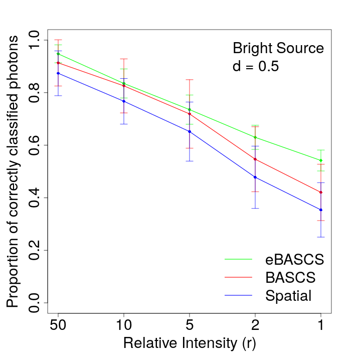
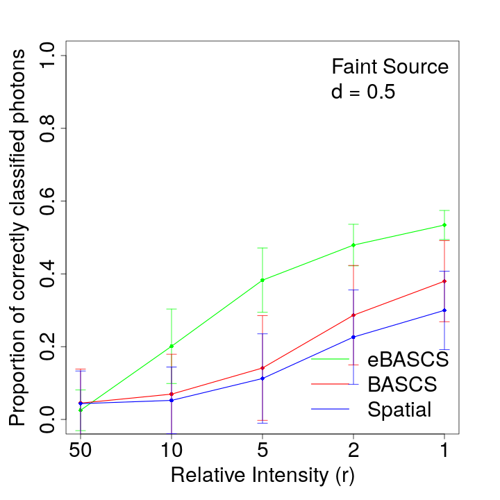
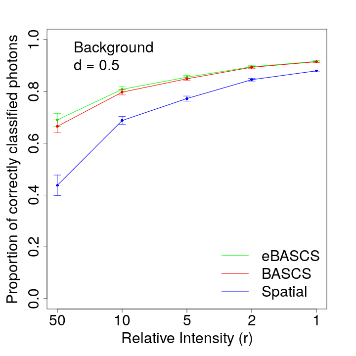
Figure 11: Allocation recovery for the bright source (left), faint source (middle) and background (right) by eBASCS (green), BASCS (red) and spatial (blue), for simulation settings $(d=0.5,r\in\{1,2,5,10,50\})$, averaged over the replicate data sets.

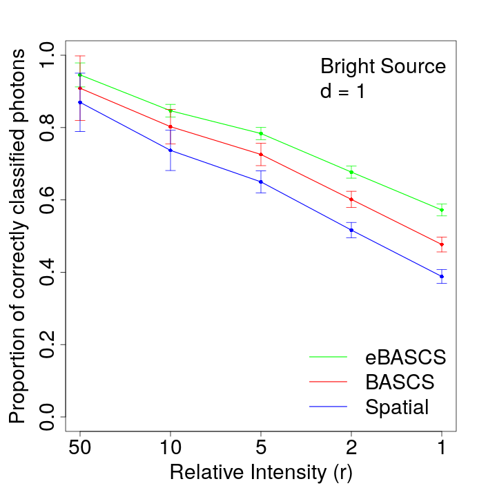
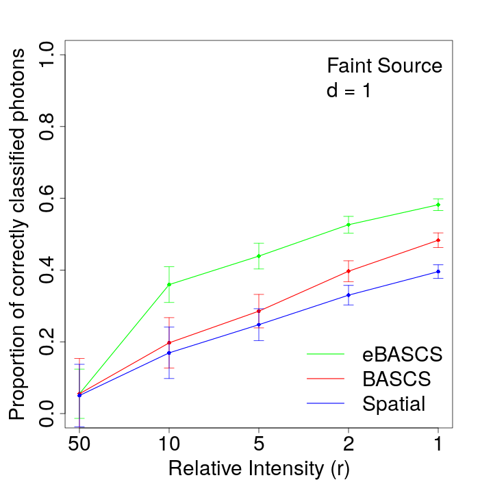
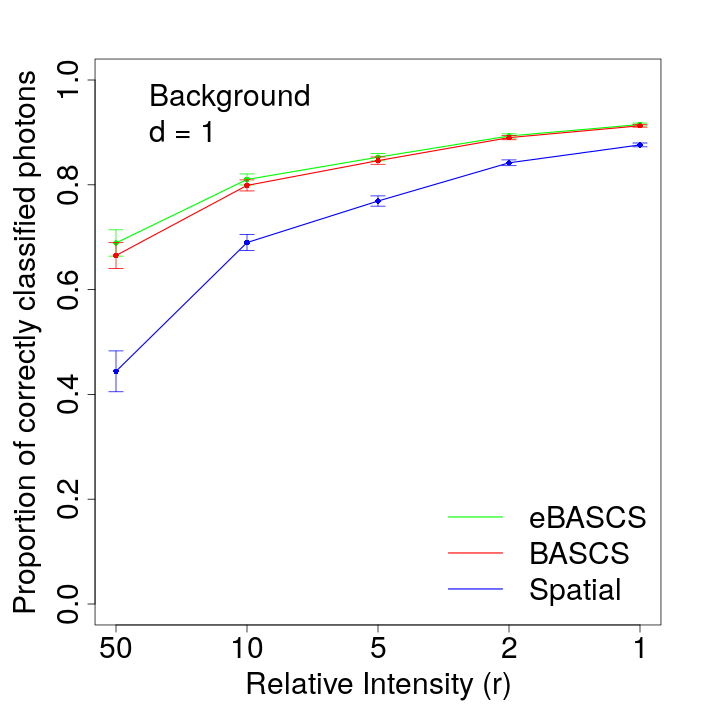
Figure 12: As in Figure 11, for $d=1$.

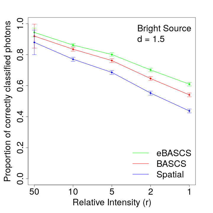
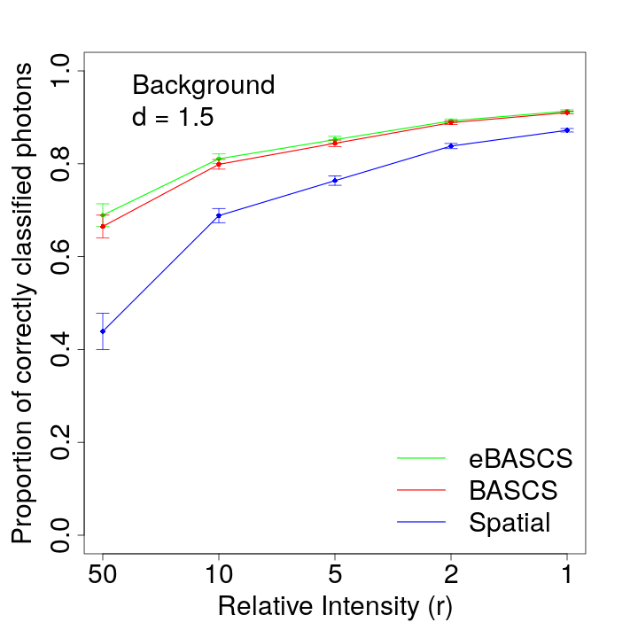
Figure 13: As in Figure 11, for $d=1.5$.

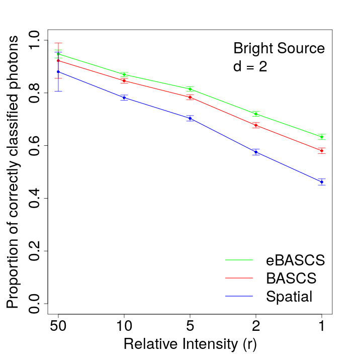
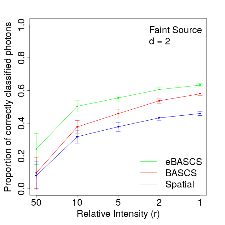
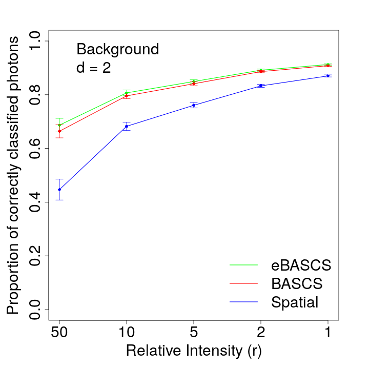
Figure 14: As in Figure 11, for $d=2$.

Appendix D Simulation I Results

D.1 Simulation I Allocation Recovery (fraction of events from a component that are correctly allocated to the same component)

Tables 9, 11, 13 give the allocation recovery of eBASCS for the bright source, faint source and background respectively. Tables 11, 11, 13 give the allocation recovery of BASCS for the bright source, faint source and background respectively. Tables 15, 15, 16 give the allocation recovery of spatial for the bright source, faint source and background respectively.

	$r$=50	$r$=10	$r$=5	$r$=2	$r$=1
$d$=0.5	0.948	0.835	0.735	0.630	0.542
$d$=1	0.946	0.846	0.784	0.677	0.572
$d$=1.5	0.943	0.862	0.801	0.701	0.610
$d$=2	0.947	0.870	0.816	0.720	0.633

Table 8: Allocation recovery for the bright source by eBASCS, averaged over MCMC iterates and replicate data sets.

	$r$=50	$r$=10	$r$=5	$r$=2	$r$=1
$d$=0.5	0.913	0.826	0.719	0.547	0.420
$d$=1	0.909	0.802	0.726	0.601	0.477
$d$=1.5	0.920	0.835	0.762	0.646	0.540
$d$=2	0.922	0.846	0.783	0.677	0.580

Table 9: As in Table 9, for BASCS.

	$r$=50	$r$=10	$r$=5	$r$=2	$r$=1
$d$=0.5	0.025	0.201	0.383	0.479	0.534
$d$=1	0.055	0.359	0.439	0.526	0.582
$d$=1.5	0.143	0.436	0.502	0.569	0.610
$d$=2	0.246	0.503	0.555	0.606	0.633

Table 10: As in Table 9, for the faint source.

	$r$=50	$r$=10	$r$=5	$r$=2	$r$=1
$d$=0.5	0.045	0.070	0.141	0.287	0.380
$d$=1	0.055	0.197	0.285	0.397	0.483
$d$=1.5	0.060	0.286	0.378	0.477	0.541
$d$=2	0.097	0.378	0.456	0.537	0.580

Table 11: As in Table 9, for the faint source by BASCS.

	$r$=50	$r$=10	$r$=5	$r$=2	$r$=1
$d$=0.5	0.690	0.808	0.855	0.895	0.916
$d$=1	0.689	0.810	0.853	0.893	0.915
$d$=1.5	0.689	0.811	0.852	0.892	0.913
$d$=2	0.686	0.807	0.849	0.891	0.913

Table 12: As in Table 9, for the background.

	$r$=50	$r$=10	$r$=5	$r$=2	$r$=1
$d$=0.5	0.665	0.797	0.849	0.893	0.914
$d$=1	0.665	0.799	0.846	0.890	0.913
$d$=1.5	0.665	0.799	0.844	0.888	0.910
$d$=2	0.664	0.796	0.841	0.886	0.908

Table 13: As in Table 9, for the background by BASCS.

	$r$=50	$r$=10	$r$=5	$r$=2	$r$=1
$d$=0.5	0.874	0.767	0.652	0.478	0.354
$d$=1	0.870	0.737	0.650	0.517	0.388
$d$=1.5	0.879	0.770	0.686	0.552	0.437
$d$=2	0.880	0.782	0.703	0.576	0.462

Table 14: As in Table 9, for spatial.

	$r$=50	$r$=10	$r$=5	$r$=2	$r$=1
$d$=0.5	0.044	0.052	0.113	0.226	0.300
$d$=1	0.050	0.170	0.248	0.330	0.396
$d$=1.5	0.050	0.247	0.319	0.392	0.437
$d$=2	0.080	0.318	0.378	0.433	0.459

Table 15: As in Table 9, for the faint source by spatial.

	$r$=50	$r$=10	$r$=5	$r$=2	$r$=1
$d$=0.5	0.437	0.688	0.772	0.845	0.879
$d$=1	0.444	0.690	0.769	0.842	0.876
$d$=1.5	0.439	0.688	0.764	0.838	0.872
$d$=2	0.447	0.682	0.761	0.833	0.870

Table 16: As in Table 9, for the background by spatial.

D.2 Simulation I Allocation Accuracy (fraction of events correctly allocated to the component)

Tables 18, 20, 22 give the allocation accuracy of eBASCS for the bright source, faint source and background respectively. Tables 18, 20, 22 give the allocation accuracy of BASCS for the bright source, faint source and background respectively. Tables 24, 24, 25 give the allocation accuracy of spatial for the bright source, faint source and background respectively.

	$r$=50	$r$=10	$r$=5	$r$=2	$r$=1
$d$=0.5	0.950	0.844	0.789	0.669	0.564
$d$=1	0.951	0.866	0.897	0.701	0.610
$d$=1.5	0.954	0.876	0.822	0.725	0.645
$d$=2	0.956	0.883	0.835	0.756	0.670

Table 17: Allocation accuracy for the bright source by eBASCS, averaged over MCMC iterates and replicate data sets.

	$r$=50	$r$=10	$r$=5	$r$=2	$r$=1
$d$=0.5	0.946	0.821	0.725	0.562	0.428
$d$=1	0.947	0.835	0.753	0.620	0.504
$d$=1.5	0.948	0.848	0.782	0.667	0.570
$d$=2	0.948	0.861	0.800	0.700	0.611

Table 18: As in Table 18, for BASCS.

	$r$=50	$r$=10	$r$=5	$r$=2	$r$=1
$d$=0.5	0.0009	0.168	0.338	0.487	0.571
$d$=1	0.016	0.363	0.456	0.550	0.608
$d$=1.5	0.078	0.459	0.535	0.603	0.641
$d$=2	0.186	0.527	0.579	0.647	0.672

Table 19: As in Table 18, for the faint source.

	$r$=50	$r$=10	$r$=5	$r$=2	$r$=1
$d$=0.5	0.010	0.031	0.109	0.301	0.422
$d$=1	0.011	0.176	0.278	0.420	0.505
$d$=1.5	0.026	0.311	0.403	0.510	0.566
$d$=2	0.063	0.394	0.479	0.565	0.614

Table 20: As in Table 18, for the faint source by BASCS.

	$r$=50	$r$=10	$r$=5	$r$=2	$r$=1
$d$=0.5	0.632	0.782	0.828	0.877	0.900
$d$=1	0.635	0.781	0.828	0.876	0.899
$d$=1.5	0.641	0.781	0.826	0.871	0.897
$d$=2	0.639	0.777	0.824	0.870	0.894

Table 21: As in Table 18, for the background.

	$r$=50	$r$=10	$r$=5	$r$=2	$r$=1
$d$=0.5	0.611	0.770	0.822	0.875	0.900
$d$=1	0.612	0.770	0.824	0.874	0.897
$d$=1.5	0.618	0.771	0.818	0.868	0.894
$d$=2	0.610	0.766	0.818	0.866	0.890

Table 22: As in Table 18, for the background by BASCS.

	$r$=50	$r$=10	$r$=5	$r$=2	$r$=1
$d$=0.5	0.922	0.770	0.665	0.492	0.358
$d$=1	0.923	0.783	0.693	0.549	0.430
$d$=1.5	0.923	0.797	0.719	0.594	0.489
$d$=2	0.927	0.811	0.739	0.618	0.515

Table 23: As in Table 18, by spatial.

	$r$=50	$r$=10	$r$=5	$r$=2	$r$=1
$d$=0.5	0.007	0.013	0.102	0.236	0.352
$d$=1	0.005	0.142	0.251	0.368	0.434
$d$=1.5	0.014	0.268	0.355	0.436	0.481
$d$=2	0.041	0.357	0.424	0.484	0.516

Table 24: As in Table 18, for the faint source by spatial.

	$r$=50	$r$=10	$r$=5	$r$=2	$r$=1
$d$=0.5	0.347	0.637	0.730	0.815	0.853
$d$=1	0.347	0.635	0.726	0.809	0.849
$d$=1.5	0.344	0.634	0.719	0.802	0.843
$d$=2	0.352	0.627	0.717	0.796	0.836

Table 25: As in Table 18, for the background by spatial.

Appendix E Simulation I: Sensitivity of posterior source location to parameter settings

Figures 16 and 16 show the true location of sources and their mean posterior locations under eBASCS (top part) and BASCS (bottom part) for all data set replicates under the simulation parameter setting indicated in the top left corner of the plot (for Simulation I). Each dot represents the mean posterior location of the source (blue for bright source, red for faint source) for one dataset replicate, and the large "X"’s of corresponding color indicate the true locations.

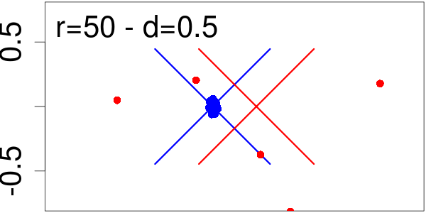
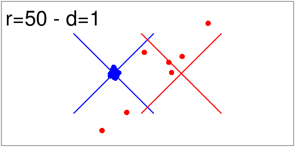
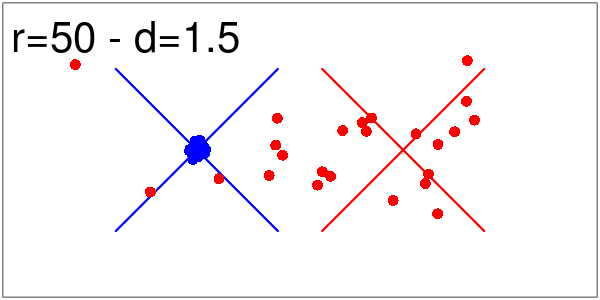
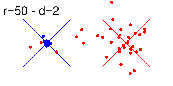
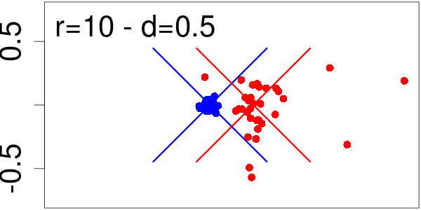
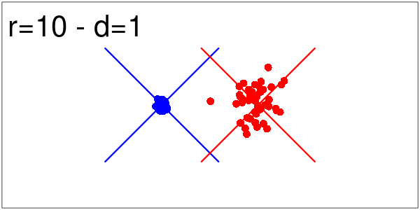
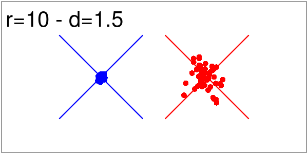
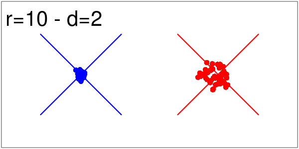
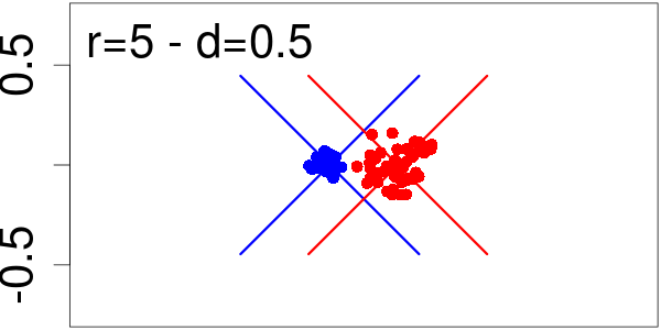
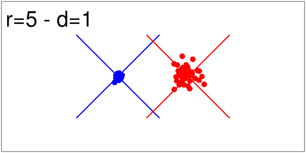
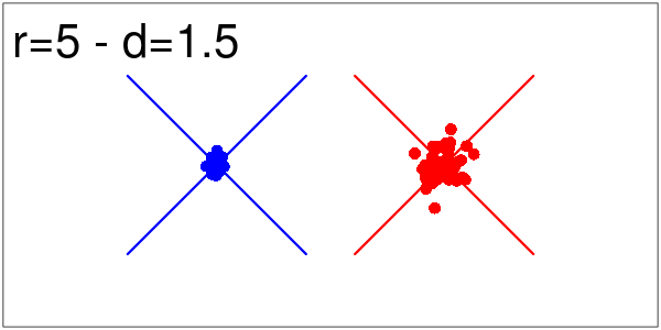
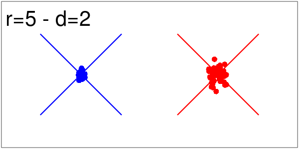
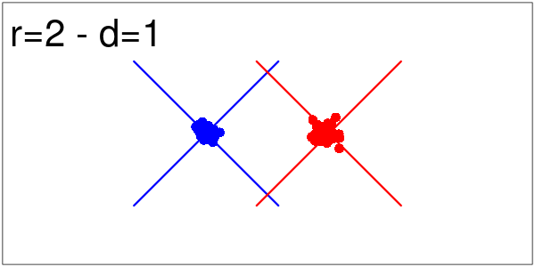
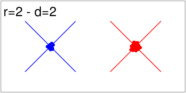
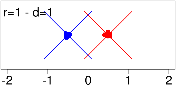
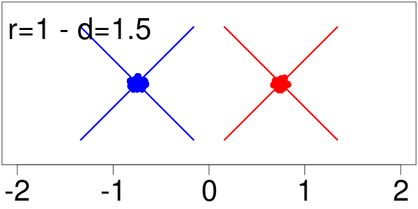
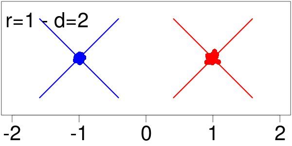
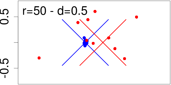
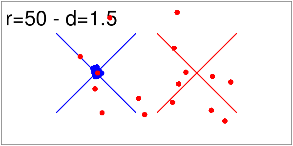
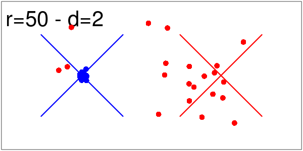
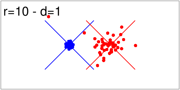
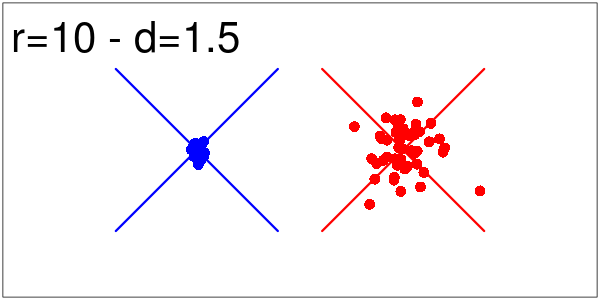
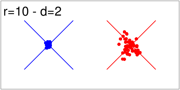
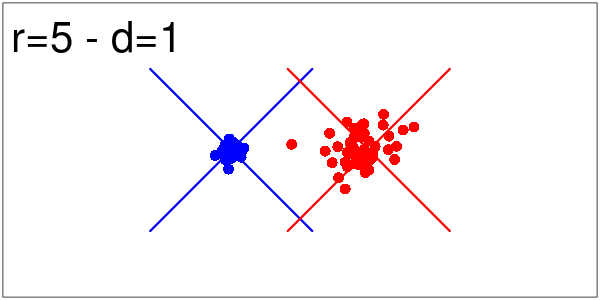
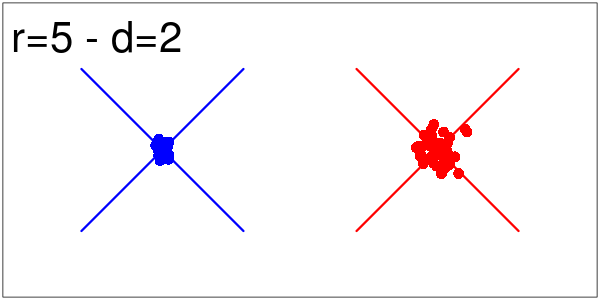
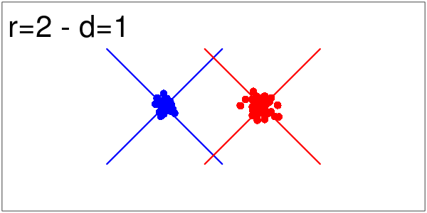
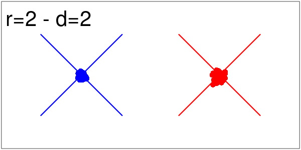
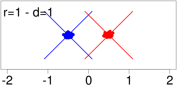
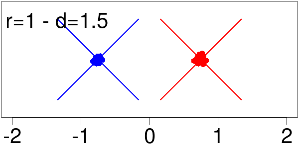
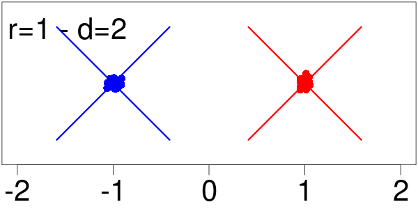
Figure 15: Sensitivity of location determination under eBASCS as a function of source separation ($d$) and relative strength ($r$). Red and blue dots give the mean posterior locations for each dataset replicate of the bright and faint sources, respectively, under the simulation setting indicated in the top-left corner of the box. The large “X”s of corresponding color indicate the true locations.

Figure 16: As in Figure 16, for BASCS.

Appendix F Simulation I: Parameter Estimates

Table 26 shows the true and estimated parameter values for a single dataset replicate under the simulation settings $d=0.5,r=1$, for the Simulation I. The posterior means of the fitted location and intensity parameters are closer to their respective true values when inferred by eBASCS compared to BASCS and spatial. The posterior quantile intervals are also narrower for eBASCS. This shows that eBASCS is able to estimate the model parameters shared with BASCS and spatial more accurately and more confidently.

		eBASCS		BASCS		spatial
	Truth	mean	(q16,q84)	mean	(q16,q84)	mean	(q16,q18)
$x_{1}$	-0.25	-0.257	(-0.30,-0.210)	-0.270	(-0.358, -0.189)	-0.279	(-0.365 , -0.192)
$y_{1}$	0	0.032	(0.006,0.058)	0.037	(-0.008,0.081)	0.046	(-0.005,0.097)
$x_{2}$	0.25	0.229	(0.198,0.258)	0.208	(0.152,0.271)	0.189	(0.134,0.245)
$y_{2}$	0	0.025	(0.002,0.047)	0.019	(-0.014,0.052)	0.022	(-0.010,0.054)
$w_{1}$	0.138	0.121	(0.105,0.136)	0.113	(0.079,0.146)	0.099	(0.068,0.130)
$w_{2}$	0.138	0.145	(0.130,0.161)	0.153	(0.120,0.187)	0.156	(0.126,0.187)
$w_{3}$	0.724	0.734	(0.729,0.739)	0.734	(0.729,0.739)	0.745	(0.739,0.750)
$\gamma_{1}$	1832	1778.132	(1732.254,1825.486)	1831.655	(1821.378,1841.74)	*	*
$\alpha_{1}$	3.18	3.212	(3.017,3.407)	3.313	(3.166,3.519)	*	*
$\gamma_{2}$	1832	1871.892	(1831.783,1911.981)	1831.113	(1817.616,1843.494)	*	*
$\alpha_{2}$	3.18	3.336	(3.158,3.512)	3.208	(3.121,3.323)	*	*
$\lambda_{1,1}$	0.05	0.039	(0.011,0.069)	*	*	*	*
$\lambda_{1,2}$	0.15	0.199	(0.170,0.227)	*	*	*	*
$\lambda_{1,3}$	0.3	0.291	(0.262,0.318)	*	*	*	*
$\lambda_{1,4}$	0.5	0.471	(0.433,0.508)	*	*	*	*
$\lambda_{2,1}$	0.5	0.511	(0.465,0.557)	*	*	*	*
$\lambda_{2,2}$	0.3	0.234	(0.210,0.258)	*	*	*	*
$\lambda_{2,3}$	0.15	0.160	(0.134,0.186)	*	*	*	*
$\lambda_{2,4}$	0.05	0.095	(0.060,0.130)	*	*	*	*
$\lambda_{3,1}$	0.25	0.245	(0.240,0.249)	*	*	*	*
$\lambda_{3,2}$	0.25	0.252	(0.247,0.256)	*	*	*	*
$\lambda_{3,3}$	0.25	0.257	(0.252,0.261)	*	*	*	*
$\lambda_{3,4}$	0.25	0.247	(0.242,0.252)	*	*	*	*

Table 26: eBASCS (left), BASCS (middle) and spatial (right) parameter estimates, resulting from an application of the models to a simulation dataset with settings $d=0.5,r=1$. Parameters $x_{j}$ and $y_{j}$ denote the spatial coordinates of the sources, $w_{j}$ their relative intensities ($j=1$ corresponds to the bright source, $j=2$ to the faint source and $j=3$ to the background). $\gamma_{j}$ and $\alpha_{j}$ respectively denote the mean and shape parameters of the gamma distributions. $\lambda_{j,k}$ denotes the relative time intensity of source $j$ in time bin $k$. The "truth" column gives the parameters values used to generate the data. The "mean" column gives the posterior mean of the corresponding parameters, and the "(q16,q84)" column reports the 16$\%$ and 84$\%$ posterior quantiles.

Appendix G Simulation II Results

G.1 Simulation II: Allocation Recovery

Tables 28, 28, 30 and 30 give the allocation recoveries of eBASCS, BASCS, spatial and space+time (respectively) in Simulation II.

	$r$=50	$r$=10	$r$=5	$r$=2	$r$=1
Bright Source	0.955	0.917	0.883	0.826	0.763
Faint Source	0.077	0.410	0.539	0.682	0.766
Background	0.616	0.609	0.588	0.560	0.525

Table 27: Allocation recovery by eBASCS, averaged over MCMC iterates and replicate data sets.

	$r$=50	$r$=10	$r$=5	$r$=2	$r$=1
Bright Source	0.926	0.889	0.837	0.738	0.631
Faint Source	0.057	0.197	0.331	0.509	0.638
Background	0.592	0.596	0.579	0.557	0.525

Table 28: As in Table 28, for BASCS.

	$r$=50	$r$=10	$r$=5	$r$=2	$r$=1
Bright Source	0.892	0.862	0.812	0.719	0.617
Faint Source	0.061	0.186	0.323	0.496	0.624
Background	0.335	0.337	0.313	0.289	0.251

Table 29: As in Table 28, for spatial.

	$r$=50	$r$=10	$r$=5	$r$=2	$r$=1
Bright Source	0.895	0.891	0.862	0.808	0.747
Faint Source	0.148	0.404	0.524	0.666	0.751
Background	0.374	0.354	0.323	0.283	0.239

Table 30: As in Table 28, for space+time.

G.2 Simulation II: Allocation Accuracy

Tables 32, 32, 34 and 34 give the allocation accuracies of eBASCS, BASCS, spatial and space+time (respectively) in Simulation II.

	$r$=50	$r$=10	$r$=5	$r$=2	$r$=1
Bright Source	0.962	0.927	0.896	0.837	0.769
Faint Source	0.037	0.413	0.519	0.678	0.771
Background	0.564	0.551	0.519	0.503	0.478

Table 31: Allocation accuracy of eBASCS, for $d=1$, averaged over MCMC iterates and replicate datasets.

	$r$=50	$r$=10	$r$=5	$r$=2	$r$=1
Bright Source	0.960	0.903	0.850	0.747	0.638
Faint Source	0.012	0.188	0.323	0.509	0.639
Background	0.549	0.526	0.527	0.499	0.474

Table 32: As in Table 32, for BASCS.

	$r$=50	$r$=10	$r$=5	$r$=2	$r$=1
Bright Source	0.946	0.890	0.840	0.741	0.635
Faint Source	0.016	0.183	0.326	0.510	0.636
Background	0.246	0.228	0.206	0.179	0.142

Table 33: As in Table 32, for spatial.

	$r$=50	$r$=10	$r$=5	$r$=2	$r$=1
Bright Source	0.950	0.917	0.890	0.830	0.765
Faint Source	0.050	0.410	0.513	0.673	0.764
Background	0.284	0.252	0.236	0.187	0.144

Table 34: As in Table 32, for space+time.

Appendix H HBC 515 A parameter estimates

Table 35 compares estimates for model parameters (fitted to the HBC 515 A data) shared by eBASCS and BASCS (i.e., spatial and spectral parameters).

	eBASCS		BASCS
	mean	(q16,q84)	mean	(q16,q84)
$x_{1}$	5.696	(5.688, 5.705)	5.697	(5.688, 5.704)
$y_{1}$	7.962	(7.955, 7.969)	7.961	(7.954, 7.969)
$x_{2}$	6.883	(6.871, 6.894)	6.881	(6.871, 6.895)
$y_{2}$	7.669	(7.658, 7.679)	7.670	(7.659, 7.680)
$w_{1}$	0.614	(0.607, 0.622)	0.615	(0.607, 0.622)
$w_{2}$	0.386	(0.378, 0.393)	0.385	(0.378, 0.393)
$w_{3}$	0.000	(0.000, 0.000)	0.000	(0.000, 0.000)
$\gamma_{1,1}$	1110.309	(1092.170, 1128.832)	1116.860	(1094.428, 1134.366)
$\gamma_{1,2}$	2278.711	(2207.070, 2351.687)	2328.049	(2223.891, 2379.936)
$\alpha_{1,1}$	10.440	(9.675, 11.197)	10.227	(9.482, 11.042)
$\alpha_{1,2}$	3.516	(3.376, 3.655)	3.631	(3.396, 3.691)
$\gamma_{2,1}$	1110.350	(1084.721, 1135.518)	1112.911	(1077.943, 1133.171)
$\gamma_{2,2}$	2244.203	(2132.280, 2353.022)	2236.035	(2106.015, 2334.583)
$\alpha_{2,1}$	11.643	(10.339, 12.949)	11.980	(10.468, 13.490)
$\alpha_{2,2}$	3.680	(3.459, 3.892)	3.673	(3.447, 3.867)
$\pi_{1}$	0.601	(0.572, 0.630)	0.612	(0.578, 0.641)
$\pi_{2}$	0.627	(0.583, 0.671)	0.619	(0.571, 0.665)

Table 35: HBC 515 A fitted spatial and spectral parameters under eBASCS (left) and BASCS (right). $x_{j}$ and $y_{j}$ denote the spatial coordinates of source $j$, $w_{j}$ denotes the relative intensity. $\gamma_{j,l}$ denotes the mean parameter of the $l^{th}$ gamma distribution component of source $j$’s spectral model (similarly with $\alpha_{j,l}$ for the shape parameter). $\pi_{j}$ denotes the mixture weight for source $j$’s mixture-of-gammas spectral model. $j=1$ corresponds to HBC 515 Aa, $j=2$ to HBC 515 Ab and $j=3$ to the background. The "mean" columns give the posterior means of the corresponding parameters, and columns "(q16,q84)" give the 16$\%$ and 84 $\%$ posterior quantiles.

Appendix I UV Ceti parameter estimates

Table 36 gives estimates for the spatial model parameters, when fitted to the UV Cet data.Table 37 gives estimates for the space+time model parameters.

	mean	q16	q84
$x_{1}$	28.074	28.052	28.096
$y_{1}$	43.503	43.481	43.525
$x_{2}$	39.008	38.975	39.042
$y_{2}$	48.199	48.164	48.235
$w_{1}$	0.659	0.654	0.664
$w_{2}$	0.286	0.282	0.291
$w_{3}$	0.055	0.052	0.058

Table 36: UV Cet fitted parameters under the spatial model. $x_{j}$ and $y_{j}$ denote the spatial coordinates of source $j$, $w_{j}$ denotes the relative intensity. $j=1$ corresponds to UV Cet B, $j=2$ corresponds to UV Cet A and $j=3$ corresponds to the background.The "mean" column gives the posterior means of the corresponding parameters, and the "(q16,q84)" column gives the 16$\%$ and 84 $\%$ posterior quantiles.

	mean	q16	q84
$x_{1}$	28.074	28.052	28.095
$y_{1}$	43.503	43.481	43.526
$x_{2}$	39.011	38.977	39.045
$y_{2}$	48.198	48.163	48.233
$w_{1}$	0.660	0.655	0.665
$w_{2}$	0.286	0.282	0.291
$w_{3}$	0.053	0.050	0.056
$\lambda_{1,1}$	0.064	0.061	0.067
$\lambda_{1,2}$	0.224	0.219	0.228
$\lambda_{1,3}$	0.102	0.099	0.105
$\lambda_{1,4}$	0.451	0.445	0.456
$\lambda_{1,5}$	0.060	0.058	0.063
$\lambda_{1,6}$	0.099	0.096	0.103
$\lambda_{2,1}$	0.395	0.386	0.404
$\lambda_{2,2}$	0.208	0.201	0.216
$\lambda_{2,3}$	0.103	0.098	0.109
$\lambda_{2,4}$	0.090	0.084	0.096
$\lambda_{2,5}$	0.139	0.133	0.145
$\lambda_{2,6}$	0.064	0.060	0.069
$\lambda_{3,1}$	0.198	0.177	0.219
$\lambda_{3,2}$	0.278	0.254	0.303
$\lambda_{3,3}$	0.115	0.098	0.133
$\lambda_{3,4}$	0.219	0.195	0.244
$\lambda_{3,5}$	0.090	0.074	0.106
$\lambda_{3,6}$	0.099	0.083	0.115

Table 37: UV Cet fitted parameters under the space+time model. $x_{j}$ and $y_{j}$ denote the spatial coordinates of source $j$, $w_{j}$ denotes the relative intensity. $\lambda_{j,k}$ denotes the relative intensity of source $j$ in time bin $k$. $j=1$ corresponds to UV Cet B, $j=2$ corresponds to UV Cet A and $j=3$ corresponds to the background.The "mean" column gives the posterior means of the corresponding parameters, and the "(q16,q84)" column gives the 16$\%$ and 84 $\%$ posterior quantiles.

References

- Akaike (1974) Akaike H., 1974, IEEE Transactions on Automatic Control, 19, 716
- Audard et al. (2003) Audard M., Güdel M., Skinner S. L., 2003, ApJ, 589, 983
- Benz et al. (1998) Benz A. O., Conway J., Gudel M., 1998, A&A, 331, 596
- Betancourt (2017) Betancourt M., 2017, arXiv e-prints, p. arXiv:1701.02434
- Carpenter et al. (2017) Carpenter B., et al., 2017, Journal of Statistical Software, Articles, 76, 1
- Davis et al. (2011) Davis R. A., Lii K.-S., Politis D. N., 2011, Remarks on Some Nonparametric Estimates of a Density Function. Springer New York, New York, NY, pp 95–100, doi:10.1007/978-1-4419-8339-8_13
- Duane et al. (1987) Duane S., Kennedy A., Pendleton B. J., Roweth D., 1987, Physics Letters B, 195, 216
- Evans et al. (2010) Evans I. N., et al., 2010, ApJS, 189, 37
- Foord et al. (2019) Foord A., et al., 2019, ApJ, 877, 17
- Freeman et al. (2002) Freeman P. E., Kashyap V., Rosner R., Lamb D. Q., 2002, ApJS, 138, 185
- Gelman et al. (2013) Gelman A., Carlin J. B., Stern H. S., Dunson D. B., Vehtari A., Rubin D. B., 2013, Bayesian Data Analysis. Chapman and Hall/CRC
- Geyer (1991) Geyer C. J., 1991, Computing Science and Statistics, Proceedings of the 23rd Symposium on the Interface, pp 156–163
- Green (1995) Green P. J., 1995, Biometrika, 82, 711
- Jones et al. (2015) Jones D. E., Kashyap V. L., van Dyk D. A., 2015, ApJ, 808, 137
- Liang & Wong (2000) Liang F., Wong W. H., 2000, Statistica Sinica, 10, 317
- Metropolis et al. (1953) Metropolis N., Rosenbluth A. W., Rosenbluth M. N., Teller A. H., Teller E., 1953, J. Chem. Phys., 21, 1087
- Neal (2011) Neal R. M., 2011, MCMC Using Hamiltonian Dynamics. CRC Press, doi:10.1201/b10905-7
- Picquenot et al. (2019) Picquenot A., Acero F., Bobin J., Maggi P., Ballet J., Pratt G. W., 2019, A&A, 627, A139
- Portillo et al. (2017) Portillo S. K. N., Lee B. C. G., Daylan T., Finkbeiner D. P., 2017, AJ, 154, 132
- Primini & Kashyap (2014) Primini F. A., Kashyap V. L., 2014, ApJ, 796, 24
- Principe et al. (2017) Principe D. A., Sacco G. G., Kastner J. H., Wilner D., Stelzer B., Micela G., 2017, A&A, 598, A8
- Reipurth et al. (2010) Reipurth B., Herbig G., Aspin C., 2010, AJ, 139, 1668
- Schwarz (1978) Schwarz G., 1978, The Annals of Statistics, 6, 461
- Sottosanti et al. (2017) Sottosanti A., Costantin D., Bastieri D., Brazzale A. R., 2017, in Convegno della Società Italiana di Statistica. pp 135–148, doi:10.1007/978-3-030-21158-5_11
- Speagle (2019) Speagle J. S., 2019, arXiv e-prints, p. arXiv:1909.12313
- Stenning & van Dyk (2021) Stenning D. C., van Dyk D. A., 2021, in , Statistics for Astrophysics. EDP Sciences, pp 29–58, doi:10.1051/978-2-7598-2275-1.c006
- Watson et al. (2009) Watson M. G., et al., 2009, A&A, 493, 339