ROmodel: Modeling robust optimization problems in Pyomo

Abstract

This paper introduces ROmodel, an open source Python package extending the modeling capabilities of the algebraic modeling language Pyomo to robust optimization problems. ROmodel helps practitioners transition from deterministic to robust optimization through modeling objects which allow formulating robust models in close analogy to their mathematical formulation. ROmodel contains a library of commonly used uncertainty sets which can be generated using their matrix representations, but it also allows users to define custom uncertainty sets using Pyomo constraints. ROmodel supports adjustable variables via linear decision rules. The resulting models can be solved using ROmodels solvers which implement both the robust reformulation and cutting plane approach. ROmodel is a platform to implement and compare custom uncertainty sets and reformulations. We demonstrate ROmodel’s capabilities by applying it to six case studies. We implement custom uncertainty sets based on (warped) Gaussian processes to show how ROmodel can integrate data-driven models with optimization.

1 Introduction

Robust optimization is a common way of managing optimization under uncertainty in process systems engineering: applications range from production scheduling to flexible chemical process design [16, 17, 29, 20, 21, 11]. New developments in robust optimization include distributionally and adjustable robust optimization to reduce solution conservatism [11], data-driven robust optimization to model uncertainty sets based on available data [4], and approximate robust optimization to make non-linear problems more tractable [14]. This large number of alternative approaches and the required domain knowledge can discourage practitioners from making the transition from deterministic optimization to optimization under uncertainty. Furthermore, the lack of a platform that allows the easy implementation and application of new algorithms means that it is difficult for researchers to compare different approaches [18].

This paper introduces ROmodel, a Python package extending the popular, Python-based algebraic modeling language Pyomo [13, 12] to facilitate modeling of robust optimization problems and implementation of robust optimization algorithms. ROmodel aims to (i) make robust optimization more accessible to practitioners and facilitate moving from deterministic to robust optimization, (ii) demonstrate how robust optimization problems can be modeled in close analogy to their mathematical formulation, and (iii) provide an open-source platform for researchers to implement and compare new robust reformulations and uncertainty sets. To this end, ROmodel introduces intuitive modeling which closely resembles the optimization problem’s underlying mathematical formulation and will feel familiar to Pyomo users. ROmodel uses the richness of Pyomo’s solver interfaces and methods for model transformations and Python’s data processing capabilities. It supports both automatic reformulation and cutting plane algorithms. Uncertainty sets can be chosen from a library of common geometries, or custom defined using Pyomo constraints. ROmodel also support adjustable robust optimization through linear decision rules. Because ROmodel and Pyomo are open-source, ROmodel can be extended to incorporate additional uncertainty set geometries and reformulations. As an example, we implemented uncertainty sets based on (warped) Gaussian processes for black-box constrained problems.

There are other software packages for solving robust optimization problems, e.g. ROME[9], RSOME[7], ROC++[23], and PyROS[15]. All four approaches are designed as robust optimization solvers and, except for PyROS which is based on Pyomo, do not rely on a general purpose algebraic modeling language. In contrast, ROmodel focuses on modeling robust optimization problems. By building on Pyomo, ROmodel simplifies the transition from deterministic to robust optimization, since both the deterministic and robust model can be implemented in the same environment. ROmodel also allows access to a much larger number of deterministic solvers than these other solvers. In contrast to AIMMS, which has some capabilities for modeling robust optimization problems [1], ROModel is open source and allows possibilities for extension. JumPeR [8], which extends Julia’s modeling language JumP to robust optimization problems, is the most similar to ROModel. In contrast to JumPeR, ROModel is more tightly tied to its respective algebraic modeling language, e.g. developing new convex uncertainty sets in ROmodel only requires adding Pyomo constraints while JumPeR would require adding Julia functionality. ROmodel also automatically recognizes uncertainy set geometries and applies the corresponding transformations without the user having to specify which geometry they are using.

A further advantage of ROmodel is that it is based on Python, which is popular in data analytics and machine learning. ROmodel therefore allows data-based techniques to be integrated seemlesly with robust optimization methods. As an example, we implement (warped) Gaussian process-based uncertainty sets in ROmodel[26]. These sets seemlesly integrate Gaussian processes trained in the Python library GPy [10] into robust optimization problems. ROmodel is open source and available on Github [28].

The rest of this paper is structured as follows. Section 2 introduces ROmodel’s new modeling objects and shows how they can be used to model robust optimization problems. Section 3 introduces ROmodel’s three solvers: a reformulation based solver, a cutting plane solver, and a nominal solver for obtaining nominal solutions of robust problems. Section 4 discusses how ROmodel can be extended and demonstrates our implementation of Gaussian process-based uncertainty sets for black-box constrained problems. Section 5 introduces six case studies and presents results.

2 Modeling

Consider the following generic deterministic optimization problem

$$\min\limits_{\boldsymbol{x}\in\mathcal{X},\boldsymbol{y}}\quad f(\boldsymbol{x},\boldsymbol{y},\bar{\boldsymbol{\xi}})$$ (1a)

s.t $$g(\boldsymbol{x},\boldsymbol{y},\bar{\boldsymbol{\xi}})\leq 0$$ (1b)

where $\boldsymbol{x}\in\mathbb{R}^{n}$ and $\boldsymbol{y}\in R^{m}$ are decision variables and $\bar{\boldsymbol{\xi}}\in\mathbb{R}^{k}$ is a vector of (nominal) parameters. If the parameter vector $\bar{\boldsymbol{\xi}}$ is not known exactly, we can construct the following robust version of Problem 1:

$$\min\limits_{\boldsymbol{x}\in\mathcal{X},\boldsymbol{y}(\boldsymbol{\xi})}\max\limits_{\boldsymbol{\xi}\in\mathcal{U}(\boldsymbol{x})}\quad f(\boldsymbol{x},\boldsymbol{y}(\boldsymbol{\xi}),\boldsymbol{\xi})$$ (2a)

s.t $$g(\boldsymbol{x},\boldsymbol{y}(\boldsymbol{\xi}),\boldsymbol{\xi})\leq 0 \forall\boldsymbol{\xi}\in\mathcal{U}(\boldsymbol{x})$$ (2b)

Here $\boldsymbol{x}\in\mathbb{R}^{n}$ are ”here and now” variables, determined before the uncertainty is revealed, while $\boldsymbol{y}(\boldsymbol{\xi})$ are adjustable variables, determined after the uncertainty is revealed. The uncertain parameter vector $\boldsymbol{\xi}$ is bounded by the uncertainty set $\mathcal{U}(\boldsymbol{x})$, which may depend on $\boldsymbol{x}$ and which contains the nominal values $\bar{\boldsymbol{\xi}}$ from Problem 1. Optimization Problem 2, a generic robust optimization problem with uncertainty in the objective and constraints, is the basis for ROmodel. Note that we are limiting ourselves here to one uncertain constraint for simplicity of notation only, ROmodel can handle multiple robust constraints. Also note that there can be an arbitrary number of deterministic constraints which define the set $\mathcal{X}$.

ROmodel introduces three new modeling objects to represent robust optimization problems like Problem 2 within Pyomo:

1. UncParam: A class similar to Pyomo’s Param and Var class used to model uncertain parameters $\boldsymbol{\xi}$. One can supply a nominal argument, which defines the vector of nominal values $\bar{\boldsymbol{\xi}}$ used to replace the uncertain parameters when solving the deterministic (nominal) problem (Eq. 1).

2. UncSet: Each UncParam object has an UncSet object associated with it. The UncSet class, based on Pyomo’s Block class, models the uncertainty sets $\mathcal{U}$. Uncertainty sets $\mathcal{U}$ can be defined by (i) constructing generic sets by adding Pyomo constraints to the UncSet object, or (ii) through a library of common uncertainty set geometries, using their matrix representation as an input.

3. AdjustableVar: A class similar to Pyomo’s Var class used to model adjustable variables which can be determined after some of the uncertainty has been resolved, i.e. $\boldsymbol{y}(\boldsymbol{\xi})$.

These three new modeling objects are sufficient for modeling quite generic robust optimization problems. They are set up to allow modeling problems in an intuitive way which is closely related to their mathematical formulation (Problem 2). We discuss each modeling object and how it is used to construct robust optimization problems in the subsequent sections.

2.1 Uncertain Parameters

Indexed uncertain parameters are constructed in analogy to Pyomo’s Var type for variables:

⬇

1 m.c = UncParam(range(3), nominal=[0.1, 0.2, 0.3], uncset=m.U)

The nominal argument specifies a list of nominal values $\bar{\boldsymbol{\xi}}$ for the uncertain paramters $\boldsymbol{\xi}$. The uncset argument specifies the uncertainty set to use for these parameters. The two approaches for constructing the uncertainty set m.U are dicussed in the next two chapters.

2.2 Generic uncertainty sets

Generic uncertainty sets are constructed with the UncSet class. This class inherits from Pyomo’s Block class. Users can construct generic uncertainty sets by adding Pyomo constraints to an UncSet object in the same way as they would add constraints to a Block object in Pyomo. The following example shows how a polyhedral set can be modeled using the UncSet class:

⬇

1 from romodel import UncSet, UncParam

2 # Define uncertainty set

3 m.U = UncSet()

4 # Define uncertain parameter

5 m.w = UncParam(range(2), uncset=m.U, nominal=[0.5, 0.5])

6 # Add constraints to uncertainty set

7 m.U.cons1 = Constraint(expr=m.w[0] + m.w[1] <= 1)

8 m.U.cons2 = Constraint(expr=m.w[0] - m.w[1] <= 1)

9 ...

The uncset and nominal arguments define the uncertainty set and a vector of nominal values for the uncertain parameter m.w. ROmodel’s strategy of modeling uncertainty sets using Pyomo’s Constraint modeling object is analogous to typical robust optimization formulations. ROmodel can therefore be used to define any uncertainty set which can be expressed in Pyomo. However, not every set that can be modeled with Pyomo constraints can necessarily also be solved. Section 3 discusses which types of uncertainty sets can be solved using which solver in. Users can also define multiple uncertainty sets and replace one by another:

⬇

1 # Define second uncertainty set

2 m.U2 = ro.UncSet()

3 # Swap uncertainty sets and solve

4 m.coef.uncset = m.U2

5 solver = pe.SolverFactory(’romodel.cuts’)

6 solver.solve(m)

2.3 Library uncertainty sets

For commonly used, standard uncertainty sets, the generic approach (Section 2.2) is unnecessarily complicated. Therefore, ROmodel implements custom classes which can define an uncertainty set using its matrix representation. ROmodel implements polyhedral and ellipsoidal sets. The user can define polyhedral sets of the form $\mathcal{U}=\left\{w\;|\;Pw\leq b\right\}$ by passing the matrix $P$ and the right hand side $b$ to the PolyhedralSet class:

⬇

1 from romodel.uncset import PolyhedralSet

2 # Define polyhedral set

3 m.U = PolyhedralSet(mat=[[ 1, 1],

4 [ 1, -1],

5 [-1, 1],

6 [-1, -1]],

7 rhs=[1, 1, 1, 1])

ROmodel creates ellipsoidal sets of the form $(w-\mu)\Sigma^{-1}(w-\mu)\leq 1$ using the EllipsoidalSet class, the covariance matrix $\Sigma$ and the mean vector $\mu$:

⬇

1 from romodel.uncset import EllipsoidalSet

2 # Define ellipsoidal set

3 m.U = EllipsoidalSet(cov=[[1, 0, 0],

4 [0, 1, 0],

5 [0, 0, 1]],

6 mean=[0.5, 0.3, 0.1])

In Section 4 we discuss how additional library sets can be added to ROmodel using data-driven uncertainty sets based on (warped) Gaussian processes as an example.

2.4 Constructing uncertain constraints

After defining uncertain parameters and an uncertainty set, the user can construct uncertain constraints implicitly by using the uncertain parameters in a Pyomo constraint. Consider the following deterministic Pyomo constraint:

⬇

1 # deterministic

2 m.x = Var(range(3))

3 c = [0.1, 0.2, 0.3]

4 m.cons = Constraint(expr=sum(c[i]*m.x[i] for i in m.x) <= 0)

If the coefficients $c$ are uncertain, we can model the robust constraint $c^{T}x\leq 0,\;\forall c\in\mathcal{U}$ as:

⬇

1 # robust

2 m.x = Var(range(3))

3 m.c = UncParam(range(3), nominal=[0.1, 0.2, 0.3], uncset=m.U)

4 m.cons = Constraint(expr=sum(m.c[i]*m.x[i] for i in m.x) <= 0)

The uncertain parameter m.c can be used in Pyomo constraints in the same way as Pyomo Var or Param objects. ROmodel’s solvers automatically recognize constraints and objectives containing containing uncertain parameters.

2.5 Adjustable variables

ROmodel also has capabilities for modeling adjustable variables. Adjustable variables $\boldsymbol{y}\left(\boldsymbol{\xi}\right)$ are variables which can be determined after some (or all) of the uncertainty has been revealed. Defining an adjustable variable is analogous to defining a regular variable in Pyomo, with an additional uncparam argument specifying a list of uncertain parameters which the adjustable variable depends on:

⬇

1 # Define uncertain parameters

2 m.w = UncParam(range(3), nominal=[1, 2, 3])

3 # Define adjustable variable which depends on uncertain parameter

4 m.y = AdjustableVar(range(3), uncparams=[m.w], bounds=(0, 1))

The uncertain parameters can also be set individually for each element of the adjustable variables index using the set_uncparams function:

⬇

1 # Set uncertain parameters for individual indicies

2 m.y[0].set_uncparams([m.w[0]])

3 m.y[1].set_uncparams([m.w[0], m.w[1]])

ROmodel only implements linear decision rules for solving adjustable robust optimization problems. If a model contains adjustable variables in a constraint or objective, ROmodel automatically replaces it by a linear decision rule based on the specified uncertain parameters.

3 Solvers

ROmodel has three solvers: A robust reformulation based solver, a cutting plane based solver, and a nominal solver.

3.1 Reformulation

The reformulation-based solver, illustrated in Fig. 1, implements standard duality based techniques for reformulating robust optimization problems into deterministic counterparts [5].

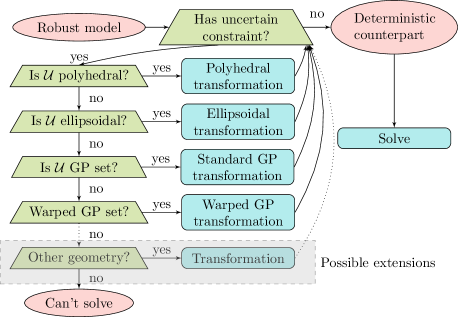
Figure 1: Schematic of reformulation solver. For each uncertain constraint, the reformulation solver goes through all known transformations and identifies the geometry of the constraint/uncertainty set. It then applies the corresponding model transformation. If all uncertain constraints can be reformulated, the resulting deterministic counterpart is solved using one of Pyomo’s solver interfaces. If one or more constraints cannot be reformulated, the problem cannot be solved.

First, it detects every constraint containing uncertain parameters. Second, it checks the structure of each uncertain constraint and the corresponding uncertainty set to determine if a known reformulation is applicable. Finally, it applies a model transformation, generating the deterministic counterpart of each robust constraint. The deterministic counterpart is then solved using an appropriate solver available in Pyomo. The structure of the optimization problem and the uncertainty set geometry determine which solvers are applicable. If no applicable transformation can be identified for one or more constraints, the problem cannot be solved and ROmodel will raise an error.

ROmodel implements standard reformulations for ellipsoidal and polyhedral uncertainty sets and linear uncertain constraints [3, 5]. It also implements reformulations for black-box constrained problems [26]. These are discussed in more detail in Section 4, which also dicussed how ROmodel can be extended to include further reformulations.

3.2 Cutting planes

The cutting plane solver, outlined in Fig. 2, implements an iterative strategy for solving robust optimization problems [19]. It replaces each uncertain constraint and objective by a CutGenerator object which initially just contains the nominal constraint. The solver then iteratively solves the master problem and generates cuts to cut off solutions which are not robustly feasible.

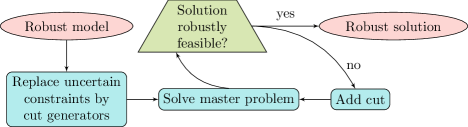
Figure 2: Schematic of cutting plane solver. The cutting plane solver iteratively solves the master problem and adds cutting planes until a robustly feasible solution is found.

A solution $x^{*}$ is considered to be robustly feasible when for each uncertain constraint $g(\boldsymbol{x}^{*},\boldsymbol{y}(\boldsymbol{\xi}),\boldsymbol{\xi})\leq 0$, the objective value of the separation problem is smaller than some tolerance $\epsilon$:

$$\max\limits_{\boldsymbol{\xi}\in\mathcal{U}}\; g(\boldsymbol{x}^{*},\boldsymbol{y}(\boldsymbol{\xi}),\boldsymbol{\xi})\leq\epsilon$$ (3)

ROmodel’s cutting plane solver can generally be applied to any convex uncertainty set. The Pyomo solvers for solving the master and separation problems can be set individually using:

⬇

1 solver = SolverFactory(’romodel.cuts’)

2 # Master solver

3 solver.options[’solver’] = ’gurobi’

4 # Sub solver

5 solver.options[’subsolver’] = ’ipopt’

The solvers need to be appropriate for the corresponding problem, i.e., the above choice would be sensible if the master problem is a mixed-integer linear problem and the uncertain constraints and uncertainty set are continuous and convex. If the solvers are not appropriate, Pyomo will raise an error.

3.3 Nominal

ROmodel also includes a nominal solver. This solver replaces all occurrences of the uncertain parameters by their nominal values and solves the resulting deterministic problem:

⬇

1 # Obtaining the nominal solution

2 solver = SolverFactory(’romodel.nominal’)

3 solver.solve(m)

The nominal solver allows users to combine their implementations of the nominal and robust problem. An implementation of the robust model can be used to obtain the solution of the nominal problem.

4 Extending ROmodel for black-box constrained problems

ROmodel can be extended to incorporate additional reformulations and uncertainty set geometries. This section outlines how ROmodel can be extended using (warped) Gaussian process-based uncertainty sets for black-box constrained problems as an example. This example showcases the ease with which ROmodel can integrate Python’s machine learning and data analytics capabilities with Pyomo’s mathematical optimization modeling.

Wiebe et al. [26] propose a robust optimization-based approximation of a class of chance-constraints containing uncertain black-box functions $g(\cdot)$:

$$P\left(\sum\limits_{i}g(\boldsymbol{y}_{i})x_{i}\leq b\right)\geq 1-\alpha$$ (4)

The approach models the black-box function and associated uncertainty using a (warped) Gaussian process as a stochastic model. The standard Gaussian process is well known and commonly used as a surrogate model [6]. Warped Gaussian processes are a more flexible variant of standard Gaussian process in which observations are mapped into a latent space using a non-linear, often neural net-style warping function [22]. If a standard Gaussian process models $g(\cdot)$, the chance constraint Eq. 4 can be reformulated exactly. For the warped Gaussian process, Wiebe et al. [26] propose an approximation based on Wolfe duality.

In order to make these approaches available in ROmodel, we need to (i) implement two library uncertainty sets, GPSet and WarpedGPSet, which collect the relevant data, and (ii) implement two corresponding model transformations which perform the reformulations for standard and warped Gaussian process-based sets. The implementation is based on the Python module ROGP [25], which is includes Gaussian process models trained in the Python library GPY [10] in Pyomo models.

4.1 Implementing new library sets

Implementing a new library set mainly requires a new Python class collecting the necessary data. For the standard and warped Gaussian process set, this data consist of three arguments:

⬇

1 from romodel.uncset import GPSet, WarpedGPSet

2 # Define variables

3 m.y = Var([0, 1])

4 # Define uncertainty set based on standard GP

5 m.uncset_standard = GPSet(gp_standard, m.z, 0.95)

6 # Define uncertainty set based on warped GP

7 m.uncset_warped = WarpedGPSet(gp_warped, m.z, 0.95)

The first argument gp_standard/warped is a (warped) Gaussian process object trained in GPy. The second is an indexed Pyomo variable on which the GP depends, i.e. $\boldsymbol{y}$ in Eq. 4. The third parameter specifies the confidence level $1-\alpha$ with which the true parameter is contained in the uncertainty set. I.e., in this case the confidence that the true parameter vector is an element of the uncertainty set is at least 95%.

The new sets can be used in the same way as other library sets, e.g.:

⬇

1 # Define variables

2 m.x = Var([0, 1])

3 # Define uncertain parameters

4 m.w = UncParam([0, 1], uncset=m.uncset_warped)

5 # Define constraint

6 m.cons = Constraint(expr=m.x[0]*m.w[0] + m.x[1]*m.w[1] <= 1)

Constraints which use this type of uncertainty set need to be linear in the uncertain parameter. Note that the indices of m.z and m.w need to be identical in the formulation above. If the black-box function depends on more than one variable, the Gaussian process-based sets can alternatively be specified using a dictionary:

⬇

1 # Define variables

2 m.y = Var([0, 1], [’a’, ’b’])

3 # Define uncertainty set

4 y_dict = {0: [m.y[0, ’a’], m.y[0, ’b’]],

5 1: [m.y[1, ’a’], m.y[1, ’b’]]},

6 m.uncset_warped = WarpedGPSet(gp, y_dict, 0.95}

The dictionary indicates that the uncertain parameter m.w[0] depends on the variables m.z[0, ’a’] and m.z[0, ’b’] through the black-box function $g(\cdot)$, modeled in GPy by the Gaussian process gp.

Note that ROmodel’s cutting plane solver is not applicable to the Gaussian process-based sets because the sets are decision dependent. Attempting to solve a problem with one of theses sets therefore results in an error. When implementing new library sets which can be solved using cutting planes, an additional Python function generate_cons_from_lib, which generates Pyomo constraints for the uncertainty set based on the data collected by the library set, is required. For an example, see romodel/uncset/ellipsoidal.py on the ROmodel Github [28].

4.2 Implementing new reformulations

For ROmodel to be able to solve models containing the two new Gaussian process-based sets, we need to implement the corresponding reformulations. Adding new reformulations to ROmodel generally requires two Python functions: (i) a function _check_applicability which detects whether a constraint and uncertainty set have the required structure, and (ii) a function _reformulate which generates the robust counterpart. The former function is only required if the reformulation is supposed to work with generically constructed uncertainty sets as described in Section 2.2. For library sets like the Gaussian process-based sets, only the latter function is required. This function takes data describing the constraints and uncertainty set as an input and returns a Pyomo block containing the deterministic counterpart. For a full example see the implemented reformulations in romodel/reformulate/ on the ROmodel Github [28].

5 Results

We use ROmodel to model and solve six case studies:

1. A portfolio optimization problem with uncertain returns [5],

2. A knapsack problem with uncertain item weights,

3. A pooling problem instance [2] with uncertain product demands,

4. A capacitated facility location problem as an example for adjustable robust optimization, where the decision which facilities to build has to be made under demand uncertainty, while the decision from which facility to supply individual customers can be made once the uncertainty is resolved,

5. A production planning in which the price at which products can be sold depends on the amount produced through an uncertain black-box function modelled by a (warped) Gaussian process [26],

6. And a drill scheduling problem in which the equipment used to drill a well degrades at a rate which depends other drill parameters through a black-box function [26].

All examples except for the drill scheduling example are included with ROmodel and can be used as follows:

⬇

1 import romodel.example as ex

2 portfolio = ex.Portfolio()

3 knapsack = ex.Knapsack()

4 pooling = ex.Pooling()

5 facility = ex.Facility()

6 planning = ex.ProductionPlanning(alpha=0.95, warped=True)

The implementation of the drill scheduling example is separately available on Github [24]. We solve the portfolio, knapsack, pooling, and facility location problems with both the reformulation and cutting plane solver for ellipsoidal and polyhedral uncertainty sets and using both the library approach to generating uncertainty sets as well as the generic, Pyomo constraint-based approach. We solve the production planning and drill scheduling problems using the reformulation solver with uncertainty sets based on both standard and warped Gaussian processes. We solve 30 instances with different uncertainty set sizes for each case study.

		Reformulation	Cuts	Overall
Knapsack	Polyhedral	60154	40272	75385
	Ellipsoidal	60150	40183	75391
Pooling	Polyhedral	60174	40329	75173
	Ellipsoidal	60638	40331	75349
Portfolio	Polyhedral	60150	40276	75126
	Ellipsoidal	60149	41659	75129
Facility	Polyhedral	60261	13353	75588
	Ellipsoidal	601–	31275	31275
Planning	Standard	62776	400NA	72776
	Warped	68536	400NA	78536
Drilling	Standard	13646	400NA	13646
	Warped	75325	400NA	75325
Overall		60174	40330	75271

Table 1: Median time in milliseconds taken to solve the six example problems with different uncertainty set geometries. Times are shown for the reformulation and cutting plane solvers and both combined (Overall). The cutting plane solver is not applicable (NA) for Gaussian process-based sets and the reformulation solver cannot solve the facility problem with ellipsoidal sets to optimality (–).

Table 1 shows the median time in milliseconds taken to solve each problem for a given uncertainty set geometry and solver. The reformulation solver generally outperforms the cutting plane solver with median times of 74ms and 330ms respectively. An exception is the the non-linear, non-convex pooling problem with an ellipsoidal set. For this instance, the cutting plane solver achieves significantly better results, which is in line with previous work on robust pooling problems [27]. Similarly, for the facility location problem with an ellipsoidal set, the reformulation approach does not solve the problem to optimality within a 10 minute time frame, while the cutting plane solver does. For the production planning and drills scheduling examples only the reformulation solver can be applied. The Wolfe duality-based reformulation for warped Gaussian processes generally takes longer to solve than the chance-constraint reformulation for standard Gaussian processes. Note that most of this time is the time taken by the subsolvers. The transformations which ROmodel performs are generally very quick: the median transformation time across all instances is $3.2$ milliseconds, while the maximum transformation time is $1.7$ seconds.

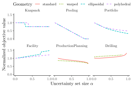
Figure 3: The figure shows the normalized objective value as a function of the uncertainty set size for knapsack, portfolio and pooling case studies and an ellipsoidal and polyhedral uncertainty set.

Fig. 3 shows the objective value (normalized with the objective of the nominal solver) as a function of uncertainty set size for each of the six examples. Note that the facility location and drill scheduling problems are minimization problems, while the rest are maximization problems. By construction, the ellipsoidal sets tested always fully contain the polyhedral sets for a given $\alpha$. Correspondingly, they are always more conservative, i.e., for a given $\alpha$ the objective value achieved using the ellipsoidal set is larger for minimization and smaller for maximization problems than the value achieved using the polyhedral set. For the Gaussian process-based sets, the standard approach is always less conservative than the warped approach. However, the limited ability of the standard Gaussian process to model non-Gaussian noise may mean that the actual probability of constraint violation is larger than the intended confidence would suggest. For a more detailed comparison of these two approaches see [26].

6 Conclusion

ROmodel formulates robust versions of common optimization problems. The modeling environment it provides makes (adjustable) robust optimization methods more readily available to practitioners and makes trying different solution approaches and uncertainty sets very easy. ROmodel is open source and available free of charge and could play a vital role as a platform for prototyping novel robust optimization algorithms and comparing them to existing approaches.

7 Acknowledgements

This work was funded by the Engineering & Physical Sciences Research Council (EPSRC) Center for Doctoral Training in High Performance Embedded and Distributed Systems (EP/L016796/1), an EPSRC/Schlumberger CASE studentship to J.W. (EP/R511961/1, voucher 17000145), and an EPSRC Research Fellowship to R.M. (EP/P016871/1).

References

- [1] AIMMS. http://aimms.com. Accessed: 2021-03-25
- [2] Adhya, N., Tawarmalani, M., Sahinidis, N.V.: A Lagrangian Approach to the Pooling Problem. Ind. Eng. Chem. Res. 38(5), 1956–1972 (1999)
- [3] Ben-Tal, A., Nemirovski, A.: Robust solutions of uncertain linear programs. Operations Research Letters 25(1), 1–13 (1999)
- [4] Bertsimas, D., Gupta, V., Kallus, N.: Data-driven robust optimization. Math. Program. 167, 235–292 (2018)
- [5] Bertsimas, D., Sim, M.: The price of robustness. Oper. Res. 52, 35–53 (2004)
- [6] Bhosekar, A., Ierapetritou, M.: Advances in surrogate based modeling, feasibility analysis, and optimization: A review. Comput. Chem. Eng. 108, 250–267 (2018)
- [7] Chen, Z., Sim, M., Xiong, P.: Robust stochastic optimization made easy with rsome. Management Science 66, 3329–3339 (2020)
- [8] Dunning, I.R.: Advances in robust and adaptive optimization: Algorithms, software, and insights. Ph.D. thesis, Sloan School of Management, MIT (2016)
- [9] Goh, J., Sim, M.: Robust optimization made easy with rome. Oper. Res. 59, 973–985 (2011)
- [10] GPy: GPy: A Gaussian process framework in python. http://github.com/SheffieldML/GPy (since 2012)
- [11] Grossmann, I.E., Apap, R.M., Calfa, B.A., García-Herreros, P., Zhang, Q.: Recent advances in mathematical programming techniques for the optimization of process systems under uncertainty. Comput. Chem. Eng. 91, 3–14 (2016)
- [12] Hart, W.E., Laird, C.D., Watson, J.P., Woodruff, D.L., Hackebeil, G.A., Nicholson, B.L., Siirola, J.D.: Pyomo — Optimization Modeling in Python, vol. 67. Springer International Publishing (2017)
- [13] Hart, W.E., Watson, J.P., Woodruff, D.L.: Pyomo: modeling and solving mathematical programs in python. Mathematical Programming Computation 3(3), 219–260 (2011)
- [14] Houska, B., Diehl, M.: Nonlinear robust optimization via sequential convex bilevel programming. Math. Program. 142, 539–577 (2013)
- [15] Isenberg, N.M., Siirola, J.D., Gounaris, C.E.: Pyros: A pyomo robust optimization solver for robust process design. In: 2020 Virtual AIChE Annual Meeting (2020)
- [16] Janak, S.L., Floudas, C.A.: Advances in robust optimization approaches for scheduling under uncertainty. Comput. Chem. Eng. 20(C), 1051–1056 (2005)
- [17] Li, Z., Ierapetritou, M.G.: Robust Optimization for Process Scheduling Under Uncertainty. Ind. Eng. Chem. Res. 47(12), 4148–4157 (2008)
- [18] Marc, A.G., Schöbel: Algorithm engineering in robust optimization. Algorithm Engineering: Selected Results and Surveys pp. 245–279 (2016)
- [19] Mutapcic, A., Boyd, S.: Cutting-set methods for robust convex optimization with pessimizing oracles. Optim. Method. Softw. 24, 381–406 (2009)
- [20] Ning, C., You, F.: A data-driven multistage adaptive robust optimization framework for planning and scheduling under uncertainty. AIChE Journal 63(10), 4343–4369 (2017)
- [21] Shang, C., You, F.: Distributionally robust optimization for planning and scheduling under uncertainty. Comput. Chem. Eng. 110, 53–68 (2018)
- [22] Snelson, E., Rasmussen, C.E., Ghahramani, Z.: Warped Gaussian processes. In: NIPS (2003)
- [23] Vayanos, P., Jin, Q., Elissaios, G.: Roc++: Robust optimization in c++. (2020)
- [24] Wiebe, J.: Drill scheduling. github.com/cog-imperial/drill-scheduling (2020)
- [25] Wiebe, J.: ROGP: Robust GPs in Pyomo. https://github.com/cog-imperial/rogp (2020)
- [26] Wiebe, J., Cecílio, I., Dunlop, J., Misener, R.: A robust approach to warped Gaussian process-constrained optimization (2020)
- [27] Wiebe, J., Cecílio, I., Misener, R.: Robust optimization for the pooling problem. Ind. Eng. Chem. Res. (2019)
- [28] Wiebe, J., Misener, R.: Romodel 0.1.0. github.com/cog-imperial/romodel (2020). DOI 10.5281/zenodo.4715841
- [29] Zhang, Q., Grossmann, I.E., Heuberger, C.F., Sundaramoorthy, A., Pinto, J.M.: Air separation with cryogenic energy storage: Optimal scheduling considering electric energy and reserve markets. AIChE Journal 61(5), 1547–1558 (2015)