Barrier and penalty methods for low-rank semidefinite programming with application to truss topology design

Abstract

The aim of this paper is to solve large-and-sparse linear Semidefinite Programs (SDPs) with low-rank solutions. We propose to use a preconditioned conjugate gradient method within second-order SDP algorithms and introduce a new efficient preconditioner fully utilizing the low-rank information. We demonstrate that the preconditioner is universal, in the sense that it can be efficiently used within a standard interior-point algorithm, as well as a newly developed primal-dual penalty method. The efficiency is demonstrated by numerical experiments using the truss topology optimization problems of growing dimension.

90C22, 90C51, 65F08, 74P05

1 Introduction

First efficient solvers for semidefinite optimization emerged more than twenty years ago. All of the general purpose solvers have been using second-order algorithms, predominantly the interior-point (IP) method. In every iteration of such an algorithm, one has to solve a system of linear equations

$$Hx=g$$

of size $n\times n$, where $n$ is the dimension of the unknown vector $x$ in the general semidefinite programming (SDP) problem

$$\min_{x\in\mathbb{R}^{n}}c^{\top}x\quad\mbox{subject to}\quad\sum_{i=1}^{{n}}x_{i}A_{i}^{(k)}-B^{(k)}\succeq 0\,,\quad k=1,\ldots,{p}$$

with $A_{i}^{(k)}\!,\;B^{(k)}\in\mathbb{R}^{{m}\times{m}}$. The assembly and solution of this linear system is a well-known bottleneck of these solvers. This is the case even for problems with sparse data and sparse linear systems, when the assembly of the system requires $\mathcal{O}\left(pnm^{3}\right)$ flops, and the solution by sparse Cholesky factorization $\mathcal{O}\left(n^{\alpha}\right)$ flops with some $\alpha\in[1,3]$.

On the other hand, many real-world applications lead to large-scale SDP, often unsolvable by current general-purpose software. There are, essentially, three ways how to approach this conundrum:

1. Reformulating the problem to make it more suitable for general-purpose solvers. This can be done, for instance, by facial reduction [22, 30, 45] or by decomposition of large matrix inequalities (and thus reducing $m$) into several smaller ones [18, 19].

2. Using a different algorithm, such as spectral bundle [14], ADMM [29], augmented Lagrangian [25, 44], optimization on manifolds [17], randomized algorithms [40] or techniques of nonlinear programming [9, 10].

3. Using one of the second-order algorithms with Cholesky factorization replaced by an iterative method for the solution of the linear systems $Hx=g$; see, e.g., [21, 37, 42].

The last approach is particularly attractive whenever $n\gg m$, and it addresses both bottlenecks of a second-order SDP solver:

• The assembly of the system matrix; an iterative solver only needs matrix-vector multiplications, and so the matrix does not have to be explicitly assembled and stored.

• The solution of the linear system itself; an iterative solver can handle very large systems, as compared to a sparse Cholesky solver, under the assumption of good conditioning of the matrix or existence of a good preconditioner.

Our goal in this paper is to design a preconditioner for the conjugate gradient (CG) method and use the resulting solver in two second-order SDP algorithms. The choice of an efficient preconditioner in a Krylov type method is problem dependent, in particular, in the context of optimization algorithms. We will focus on problems with expected very low-rank dual solutions.

SDP problems with low-rank dual solutions are common in relaxations of optimization problems in different areas such as combinatorial optimization [7], approximation theory [11, 23], control theory [23, 41], structural optimization [35], and power systems [24].

It is not our goal to find a low-rank dual solution in case of non-unique solutions; indeed, it is well-known that an interior-point method will converge to a maximal complementary solution. However, if the method will converge to a low-rank dual solution, we will use this fact to improve its computational complexity and memory demands. Our method is not only limited to problems with (theoretically exactly) low-rank solutions, it can be efficiently applied when the dual solution has a few outlying eigenvalues. Moreover, our method can be applied to problems with several linear matrix inequalities (LMIs) with different rank of the corresponding dual solutions and with bound constraints on the variable $x$, i.e., constraints that, mostly, do not exhibit low-rank duals.

There is one major difference to other algorithms for SDP problems with low-rank solutions, such as SDPLR [9, 10], optimization on manifolds [17] and other approaches [4, 40]. All these methods require the knowledge of a guaranteed (possibly tight) upper bound on the rank of the solution. If the estimate of the rank was lower than the actual rank, the algorithm would not find a solution. In our approach, the rank information is merely used to speed-up a standard, well-established algorithm. If our estimated rank is smaller than the actual one, we will only see it in possibly more iterations of the CG solver; the convergence behaviour of the optimization algorithm will be unchanged.

In this paper we present the application of the preconditioned iterative method in two second-order optimization algorithms, the “standard” primal-dual interior-point method and a new primal-dual augmented Lagrangian method (PDAL). The interior-point algorithm mimics the reliable primal-dual algorithm with Nesterov-Todd direction, as used in the SDPT3 solver [36, 37]. The augmented Lagrangian method is based on the PENNON algorithm in [20], but implements a number of useful modifications. The most important change is to solve the subproblems in the augmented Lagrangian framework by a primal-dual approach inspired by the work of Griva and Polyak [13]. For this, we rephrase the Newton’s system in the augmented Lagrangian algorithm by a primal-dual system which is then solved approximately by the preconditioned conjugate gradient (PCG) method. Additional modifications include the use of two different penalty functions for standard linear and LMI constraints—we consider a quadratic-logarithmic penalty function [5, 6, 28, 46] for standard linear constraints and a hyperbolic penalty function [20, 21] to construct primary matrix function [15] for penalizing LMI constraints—as well as the application of a regularization term in the augmented Lagrangian function which bounds the eigenvalues of the Hessian matrix uniformly away from zero.

Our preconditioner is motivated by the work of Zhang and Lavaei [42]. They present a preconditioner for the CG method within a standard IP method that makes it more efficient for large-and-sparse low-rank SDPs. We partly follow their approach though there are some major differences: we abandon a crucial assumption on sparsity of the data matrices (Assumption 2 in [42]); our method allows for SDPs with more than one LMI and with (simple) linear constraints; the complexity of computing our preconditioner is substantially lower; we can also efficiently solve problems with a few outlying eigenvalues in the optimal solution.

To test the developed algorithms, we have generated a library of problems arising from truss topology optimization without and with vibration constraints, formulated as SDP. These problems are characterized by a very low-rank solutions (1–3), additional linear (bound) constraints and scalability, in the sense that one can generate a range of problems of various dimension but of the same type. Depending on the choice of the lower bound, the solutions are either of exact very low rank or an approximate one, with a very few outlying eigenvalues. We will demonstrate that, to solve the large-scale instances, both new elements of our engines have to be employed, the very use of an iterative solver (to address the matrix assembly and related memory issues) and an efficient preconditioner (to address the efficiency of the iterative solver). This is not always the case of the large scale SDP problems; for instance, the matrix completion problem requires the use of an iterative solver (within a second-order algorithm) but no preconditioner is needed in many instances.

The paper is organized as follows. Section 2 introduces the SDP problems we want to solve and some basic assumptions. In Sections 3 and 4, PDAL and IP methods are presented. Also, in these sections, the complexity of the Schur complement system in IP and the Hessian system in PDAL are discussed. Next, in Section 5, we introduce the preconditioners. Section 6 describes our application, the truss topology optimization problems without and with vibration constraints. In the last Section 7, we present two Matlab codes, PDAL and Loraine, implementing the developed algorithms, together with results of our numerical experiments. We also give comparison with other existing SDP software and demonstrate the high efficiency of our algorithms.

Notation

We denote by $\mathbb{S}^{m},\mathbb{S}^{m}_{+}$ and $\mathbb{S}^{m}_{++}$, respectively, the space of $m\times m$ symmetric matrices, positive semidefinite and positive definite matrices. The eigenvalues of a given matrix $X\in\mathbb{S}_{++}^{m}$ are ordered as $\lambda_{1}(X)\leq\dots\leq\lambda_{m}(X)$, and its condition number is defined as $\kappa(X)=\lambda_{1}(X)/\lambda_{n}(X)$. The notation “vec” and “$\otimes$" refer to the (non-symmetrized) vectorization and Kronecker product, respectively. With this notation the following identity holds true: $\text{vec}(AXB^{\top})=(A\otimes B)\text{vec}(X)$. The symbol $\bullet$ denotes the Frobenius inner product of two matrices, $A\bullet B=\text{tr}(A^{\!\top}\!B)$.

2 Low-rank semidefinite optimization

In the first part of the paper, we consider a (primal) semidefinite optimization problem

(1) $$\min_{X\in\mathbb{S}^{m},\,x_{\text{lin}}\in\mathbb{R}^{m}\leavevmode\nobreak\ }C\bullet X+d^{\top}x_{\text{lin}}$$

$$\text{{subject to}}\ \begin{aligned} &A_{i}\bullet X+(D^{\top}x_{\text{lin}})_{i}=b_{i},\quad i=1,\dots,n\\ &X\succeq 0,\ x_{\text{lin}}\geq 0\end{aligned}$$

together with its Lagrangian dual

(2) $$\max_{y\in\mathbb{R}^{n},\;S\in\mathbb{S}^{m},s_{\text{lin}}\in\mathbb{R}^{m}\leavevmode\nobreak\ }b^{\top}y$$

$$\text{{subject to}}\leavevmode\nobreak\ \begin{aligned} &\sum_{i=1}^{n}y_{i}A_{i}+S=C\\ &Dy+s_{\text{lin}}=d\\ &S\succeq 0\\ &s_{\text{lin}}\geq 0\,.\end{aligned}$$

Here $A_{i}\in\mathbb{S}^{m}$, $i=1,\ldots,n$, $C\in\mathbb{S}^{m}$, $b\in\mathbb{R}^{n}$, $D\in\mathbb{R}^{\nu\times n}$ and $d\in\mathbb{R}^{\nu}$ are data of the problem.

While the linear constraints can be formally included in the linear matrix inequality, we write them explicitly, as they will be treated differently in the algorithms below. Later, in Section 5, we will also use a more specific notation for problems with several matrix variables.

Basic assumptions

We make the following assumptions about (1).

Assumption 2.1.

Problems Eqs. 1 and 2 are strictly feasible, i.e., there exist $X\in\mathbb{S}^{m}_{++}$, $y\in\mathbb{R}^{n}$, $S\in\mathbb{S}^{m}_{++}$, such that $A_{i}\bullet X=b_{i}$ and $\sum_{i=1}^{n}y_{i}A_{i}+S=C$ (Slater’s condition).

Assumption 2.2.

Define the matrix ${\bf A}=[\text{\rm vec}A_{1},\dots,\text{\rm vec}A_{n}]$. We assume that matrix-vector products with ${\bf A}$ and ${\bf A}^{\!\!\top}$ may each be computed in $\mathcal{O}(n)$ flops and memory.

Assumption 2.3.

The inverse $(D^{\top}D)^{-1}$ and matrix-vector product with $(D^{\top}D)^{-1}$ may each be computed in $\mathcal{O}(n)$ flops and memory.

Assumption 2.4.

The dimension of $X$ is much smaller than the number of constraints, i.e., $m\ll n$.

Remark.

2.3 is satisfied, for instance, in case of box constraints on variable $y$ in the dual formulation. 2.4 is not really needed as a “mathematical” assumption, all methods presented in the paper would work without it. However, the complexity of these methods would then be comparable with standard software using Cholesky factorization. The presented methods will be only superior to the standard software under this assumption.

Low-rank assumption

As mentioned in the Introduction, our approach is focused on linear systems with matrices having few large outlying eigenvalues. This, of course, includes matrices with very low rank but also matrices with “approximate” low rank. These matrices frequently appear in optimization algorithms, such as interior-point methods, when the “exact” low rank is only attained at the (unreached) optimum. Moreover, the approach allows us to solve problems with matrices of high rank but with a few large outlying eigenvalues, such as the problems in Section 6.

Because our approach covers SDP problems with (genuinely) low-rank solutions and for the lack of better terminology for the larger class of matrices with outlying eigenvalues, we still call our main assumption “low-rank” and the problems we are targeting “SDP problems with low-rank solutions”.

Our main assumption used in the design of an efficient preconditioner concerns the eigenvalue distribution of the solution $X^{*}$ of (1). We will assume that $X^{*}$ has a very small number of large outlying eigenvalues. This will include problems where $X^{*}$ is of a very low rank.

Assumption 2.5.

Let $X^{*}$ be the solution of (1). We assume that $X^{*}$ has $k$ outlying eigenvalues, i.e., that

$$(0\leq)\;\lambda_{1}(X^{*})\leq\cdots\leq\lambda(X^{*})_{m-k}\ll\lambda(X^{*})_{m-k+1}\leq\cdots\leq\lambda(X^{*})_{m}\,,$$

where $k$ is very small, typically smaller than 10 and, often, equal to 1.

Remark.

In order to emphasize the difference of this paper to [42]—that otherwise served as our motivation—we include the following remarks.

1. We do not assume that the matrix ${\bf A}^{T}{\bf A}$ is easily invertible. Indeed, it is not in our application in Section 6, contrary to examples in [42] where this matrix is diagonal.

2. We do not assume anything about the distribution of the first $(m-k)$ eigenvalues of $X^{*}$; they may not be equal to zero, they may not be clustered.

3. We make no assumption about the “rank” of the solution $x^{*}_{\rm lin}$ of (1), i.e., about the number of active constraints in the linear inequality $Dy\leq d$ in (2). This can be arbitrarily large or small.

3 Generalized augmented Lagrangian method

3.1 Primal approach

In this section, an augmented Lagrangian type algorithm for the solution of SDPs of type Eq. 2 is presented. Our method is based on the PENNON algorithm in [20], but implements a number of useful modifications, which help to deal with ill-conditioned data. In our algorithm, we consider the LMI in Eq. 2 without slack, i.e.,

(3) $$A^{\rm{lmi}}(y) =A_{0}(y)-C\preceq 0,$$

where $A_{0}(y)=\sum^{n}_{i=1}A_{i}y_{i}$. Moreover, we formally treat the linear constraints as a diagonal matrix inequality, i.e.,

$$A^{\rm{lin}}(y) =\textrm{diag}(Dy-d)\preceq 0,$$

and set $\tilde{b}:=-b$ in order to turn Eq. 2 into a minimization problem. In a general setting, we may have many constraints of type Eq. 3, however, for the sake of readability in this section, we assume that $A(y)$ is a block matrix with only two blocks

$$A(y)=\begin{pmatrix}A^{\rm{lmi}}(y)&0\\ 0&A^{\rm{lin}}(y)\end{pmatrix}.$$

Here, $A^{\rm{lmi}}(y)\in\mathbb{S}^{m}$ and $A^{\rm{lin}}(y)\in\mathbb{S}^{\nu}$. Moreover $A^{\rm{lin}}(y)$ is a diagonal matrix for every $y\in\mathbb{R}^{n}$ by construction, while we do not assume any particular structure for $A^{\rm{lmi}}(y)$.

The Lagrangian for the resulting problem is defined by the formula

(4) $$L(y,X)=\tilde{b}^{\top}y+A(y)\bullet X=\tilde{b}^{\top}y+A^{\rm{lmi}}(y)\bullet X^{\rm{lmi}}+A^{\rm{lin}}(y)\bullet X^{\rm{lin}},$$

where $X$ is a Lagrange multiplier in $\mathbb{S}^{m+\nu}_{+}$, which is again a block matrix composed from the blocks $X^{\rm{lmi}}\in\mathbb{S}^{m}_{+}$ and $X^{\rm{lin}}\in\mathbb{S}^{\nu}_{+}$. Next, a class of scalar-valued penalty functions is defined.

Definition 3.1.

Let $\varphi:\mathbb{R}\to\mathbb{R}$ be a real-valued penalty function having the following properties [28]:

1. $\varphi$ is a strictly decreasing twice differentiable strictly convex function of one variable with Dom $\varphi=(b,\infty),-\infty\leq b<0$,

2. $\lim_{t\rightarrow b}\varphi^{\prime}(t)=-\infty$,

3. $\lim_{t\to\infty}\varphi^{\prime}(t)=0$,

4. $\varphi(0)=0$,

5. $\varphi^{\prime}(0)=-1$.

Using Definition 3.1 and a positive penalty parameter $\pi$, we define a whole family of penalty functions

(5) $$\varphi_{\pi}(t)=\pi\,\varphi\left(\frac{t}{\pi}\right),$$

for which we observe:

$$\lim_{\pi\to 0}\varphi_{\pi}(t)=\begin{cases}\ 0,&\quad t\leq 0,\\ \ \infty,&\quad t>0.\end{cases}$$

In this paper, to penalize positive diagonal values of $A^{\rm{lin}}(y)$, we use the so called quadratic-logarithmic penalty function [28, 5, 6, 46] which is given by

$$\varphi^{\rm{qlog}}(t)=\begin{cases}-\log(1-t),&\quad t\leq\tau,\\ \frac{(1+\tau)^{3}(-t-\tau)^{4}}{4}+\frac{1}{3}\left(\frac{t+\tau}{1+\tau}\right)^{3}+\frac{1}{2}\left(\frac{-t-\tau}{1+\tau}\right)^{2}-\log(1+\tau),&\quad t>\tau,\end{cases}$$

where $\tau$ is a positive number in which the logarithmic function is extrapolated in a twice continuously differentiable way by a quadratic function.

For the linear matrix inequality constraints, i.e., the block $A^{\rm{lmi}}(y)$ we consider the hyperbolic penalty function defined as:

(6) $$\varphi^{\rm{hyp}}(t)=-\frac{1}{t-1}-1.$$

It is easy to check that properties (1–5) of Definition 3.1 are satisfied for both functions $\varphi^{\rm{qlog}},\varphi^{\rm{hyp}}$ [28, 31, 33].
Next we explain, how a penalty function from Definition 3.1 can be used to penalize positive eigenvalues of $A^{\rm{lmi}}(y)$.

Definition 3.2.

Let $\varphi:\mathbb{R}\to\mathbb{R}$ be a given function and $A\in\mathbb{S}^{m}$ be a given symmetric matrix. Let $A=S\Lambda S^{\top}$, with $\Lambda=diag(\lambda_{1},\ldots,\lambda_{m})^{\top}$ being an eigenvalue decomposition of $A$. Then the primary matrix function $\Phi_{\pi}$ corresponding to $\varphi_{\pi}$ is defined by [15]:

$$\Phi_{\pi}:\mathbb{S}^{m} \to\mathbb{S}^{m}$$

$$A \to S\begin{pmatrix}\varphi_{\pi}(\lambda_{1})&0&\cdots&0\\ 0&\varphi_{\pi}(\lambda_{2})&\,&\vdots\\ \vdots&\,&\ddots&0\\ 0&\cdots&0&\varphi_{\pi}(\lambda_{m})\end{pmatrix}S^{\top}.$$

Using this, in principle, any scalar penalty function can be turned into a matrix penalty function. The main reason why we are using the hyperbolic penalty function Eq. 6 is that for the evaluation of it, no eigenvalue decomposition is required. Instead, we can write [20]:

$$\Phi^{\rm{hyp}}_{\pi}\left(A^{\rm{lmi}}(y)\right) =\pi\left(-\left(\pi^{-1}A^{\rm{lmi}}(y)-I\right)^{-1}-I\right)=\pi^{2}\mathcal{Z}(y,\pi)-\pi I,$$

where $\mathcal{Z}(y,\pi)=-(A^{\rm{lmi}}(y)-\pi I)^{-1}$ and $I$ is the identity matrix in $\mathbb{S}^{m}$. Note that we formally also use the formalism of primary matrix functions for the diagonal block $A^{\rm{lin}}(y)$ giving rise to a matrix penalty function $\Phi^{\rm{qlog}}_{\pi}$, but of course in this case the scalar penalty function can be directly applied to the diagonal entries of $A^{\rm{lin}}(y)$, which means that also here the eigenvalue decomposition can be avoided. In the following, we use the compact notation $\Phi_{\pi}(A(y))$ with $\pi=(\pi^{\rm{lin}},\pi^{\rm{lmi}})$ for the expression

$$\begin{pmatrix}\Phi^{\rm{hyp}}_{\pi^{\rm{lmi}}}(A^{\rm{lmi}}(y))&0\\ 0&\Phi^{\rm{qlog}}_{\pi^{\rm{lin}}}(A^{\rm{lin}}(y))\end{pmatrix}.$$

Using the penalty functions $\Phi^{\rm{qlog}}_{\pi}$ and $\Phi^{\rm{hyp}}_{\pi}$, we are now able to rewrite Eq. 3 as:

(7) $$A(y)\preceq 0\Leftrightarrow\Phi_{\pi}\left(A(y)\right)\preceq 0\Leftrightarrow\Phi^{\rm{hyp}}_{\pi^{\rm{lmi}}}\left(A^{\rm{lmi}}(y)\right)\preceq 0\ \rm{and}\ \Phi^{\rm{qlog}}_{\pi^{\rm{lin}}}\left(A^{\rm{lin}}(y)\right)\preceq 0.$$

We note that this reformulation is sometimes referred to as nonlinear rescaling [13, 32]. Using this and the Lagrange formalism, we can now define the generalized augmented Lagrangian associated with Eq. 1 as:

(8) $$F(y,\bar{y},X,\pi^{\rm{lin}},\pi^{\rm{lmi}})=\tilde{b}^{\top}y+\frac{r}{2}\|y-\bar{y}\|^{2}+X\bullet\Phi_{\pi}\left(A(y)\right)$$

$$=\tilde{b}^{\top}y+\frac{r}{2}\|y-\bar{y}\|^{2}+X^{\rm{lmi}}\bullet\Phi^{\rm{hyp}}_{\pi^{\rm{lin}}}\left(A^{\rm{lmi}}(y)\right)+X^{\rm{lin}}\bullet\Phi^{\rm{qlog}}_{\pi^{\rm{lmi}}}\left(A^{\rm{lin}}(y)\right).$$

In contrast to the PENNON algorithm [20], in Eq. 8, we add a proximal point regularization term with a regularization parameter $r$, which provides a uniform lower bound for the eigenvalues of the Hessian $\nabla^{2}_{yy}F$, as will be seen later.

Next, the basic (primal) augmented Lagrangian algorithm is defined in Algorithm 1.

Algorithm 1 Generalized Augmented Lagrangian Algorithm

Let $X_{0}\in\mathbb{S}^{m+\nu}_{++}$, $\pi^{\rm{lin}}_{0}>0$, $\pi^{\rm{lmi}}_{0}>0$ and $y_{0}\in\mathbb{R}^{n}$ be given.

1:for $k=0,1,2,\ldots$ do

2:      Minimize Eq. 8 with respect to $y$ with fixed $X_{k}$ and $\pi_{k}$, i. e. compute $y_{k+1}\in\mathbb{R}^{n}$ such that:

(9) $$\nabla_{y}F(y_{k+1},y_{k},X_{k},\pi_{k}^{\rm{lin}},\pi_{k}^{\rm{lmi}})=0.$$

3:      Update the multiplier $X_{k}$:

• for the linear constraint block compute the diagonal multiplier $X^{\rm{lin}}_{k+1}$ by

  (10) $$\widetilde{X}^{\rm{lin}}_{k+1}=\bar{X}^{\rm{lin}}(y_{k+1},X^{\rm{lin}}_{k},\pi_{k}^{\rm{lin}}),$$

  with the multiplier update function

  $$\bar{X}_{i,j}^{\rm{lin}}(y,X,\pi)=\begin{cases}\ X_{i,i}\varphi^{\prime}_{\pi}(A_{i,i}^{\rm{lin}}(y)),&\quad i=j,\\ \ 0,&\quad i\neq j;\end{cases}$$

• for the LMI block compute

  (11) $$\widetilde{X}^{\rm{lmi}}_{k+1}=\bar{X}^{\rm{lmi}}(y_{k+1},X^{\rm{lmi}}_{k},\pi_{k}^{\rm{lmi}}),$$

  with the multiplier update function $\bar{X}^{\rm{lmi}}(y,X,\pi)=\pi^{2}\mathcal{Z}(y,\pi)X\mathcal{Z}(y,\pi)$, see [20];

• damp multiplier update by

  $$X^{\rm{lin}}_{k+1}=(1-\gamma^{\rm{lin}})\widetilde{X}^{\rm{lin}}_{k+1}+\gamma^{\rm{lin}}\widetilde{X}^{\rm{lin}}_{k+1},\quad X^{\rm{lmi}}_{k+1}=(1-\gamma^{\rm{lmi}})\widetilde{X}^{\rm{lmi}}_{k+1}+\gamma^{\rm{lmi}}\widetilde{X}^{\rm{lmi}}_{k+1}$$

  using algorithmic parameters $0\leq\gamma^{\rm{lin}},\gamma^{\rm{lmi}}\leq 1$.

4:      Update the penalty parameters $\pi^{\rm{lin}}_{k},\pi^{\rm{lmi}}_{k}$:

• for the linear constraint block compute

  $$\pi^{\rm{lin}}_{k+1}=\max(\pi^{\rm{lin}}_{\rm{min}},\pi_{\rm{upd}}^{\rm{lin}}\pi^{\rm{lin}}_{k});$$

• for the linear matrix inequality constraints

  $$\pi^{\rm{lmi}}_{k+1}=\max\left(\pi^{\rm{lmi}}_{\rm{min}},\pi_{\rm{upd}}^{\rm{lmi}}\pi^{\rm{lmi}}_{k},1.01\lambda_{\max}(A^{\rm{lmi}}(y_{k+1}))\right),$$

  where $\lambda_{\max}(\cdot)$ denotes the largest eigenvalue of a matrix and $0<\pi_{\rm{upd}}^{\rm{lmi}},\pi_{\rm{upd}}^{\rm{lin}}<1$, $\pi^{\rm{lmi}}_{\rm{min}},\ \pi^{\rm{lin}}_{\rm{min}}>0$ are algorithmic parameters.

5:end for

As usual in augmented Lagrangian methods, the Lagrange multiplier update in Eq. 11 is motivated as follows. From Eq. 9, we have

(12) $$\nabla_{y}F(y_{k+1},y_{k},X_{k},\pi_{k}^{\rm{lin}},\pi_{k}^{\rm{lmi}})=$$

$$\qquad\tilde{b}+r(y_{k+1}-y_{k})+A^{*}\bar{X}(y_{k+1},X_{k},\pi_{k}^{\rm{lin}},\pi_{k}^{\rm{lmi}})=0\,;$$

here, $A^{*}$ is the adjoint operator to $A$ and $\bar{X}(y_{k+1},X_{k},\pi_{k}^{\rm{lin}},\pi_{k}^{\rm{lmi}})$ is a block diagonal matrix with blocks $\bar{X}^{\rm{lin}}(y_{k+1},X_{k}^{\rm{lin}},\pi_{k}^{\rm{lin}})$ and $\bar{X}^{\rm{lmi}}(y_{k+1},X_{k}^{\rm{lmi}},\pi_{k}^{\rm{lmi}})$; see Algorithm 1. Now, inserting the updated multiplier $X_{k+1}$, the left hand side of the last equation becomes $\tilde{b}+r(y_{k+1}-y_{k})+A^{*}X_{k+1}$. For $r=0$, this implies

(13) $$\nabla_{y}L(y_{k+1},X_{k+1})=\tilde{b}+A^{*}X_{k+1}=0,$$

which means that $y_{k+1}$ is also stationary for the standard Lagrangian, if we set the proximal point parameter equal to zero. For positive $r$, this holds at least in an asymptotic sense, as $y_{k+1}-y_{k}\to 0$ for $k\to\infty$.

When we solve Step 2 of Algorithm 1 by Newton’s method, Algorithm 1 is (apart from the proximal point regularization and the special treatment of the linear constraints) essentially equivalent to the PENNON algorithm described in [20]. Before applying a few further modifications to Algorithm 1, let us have a more detailed look at the Newton iteration. For this, we need to compute the gradient and Hessian of the augmented Lagrangian Eq. 8 in each iteration. One easily verifies that the Hessian can be computed using the formula

(14) $$H_{k}(y):=\nabla^{2}_{yy}F(y,y_{k},X_{k},\pi_{k}^{\rm{lin}},\pi_{k}^{\rm{lmi}})$$

$$=rI+2\left[A_{i}\bullet\bar{X}^{\rm{lmi}}(y,X_{k}^{\rm{lmi}},\pi_{k}^{\rm{lmi}})A_{j}\mathcal{Z}(y,\pi_{k}^{\rm{lmi}})\right)]_{i,j=1}^{n}+D^{\top}\bar{W}^{\rm{lin}}(y,X_{k}^{\rm{lin}},\pi_{k}^{\rm{lin}})D$$

$$=rI+2{\bf A}^{\!\!\top}\left(\bar{X}^{\rm{lmi}}(y,X_{k}^{\rm{lmi}},\pi_{k}^{\rm{lmi}})\otimes\mathcal{Z}(y,\pi_{k}^{\rm{lmi}})\right){\bf A}+D^{\top}\bar{W}^{\rm{lin}}(y,X_{k}^{\rm{lin}},\pi_{k}^{\rm{lin}})D$$

with

(15) $$\bar{W}_{i,j}(y,X,\pi)=\begin{cases}\ X_{i,i}\varphi^{\prime\prime}_{\pi}(A_{i,i}^{\rm{lin}}(y)),&\quad i=j,\\ \ 0,&\quad i\neq j,\end{cases}$$

${\bf A}$ being the $m\times n$ matrix defined in 2.2 and $D$ being the $\nu\times n$ matrix defining the linear constraints.

Let us first look at the conditioning of the Hessian.

Lemma 3.3.

The eigenvalues of $H_{k}(y)$ are bounded from below by $r$.

Proof 3.4.

Due to the positive semidefiniteness of the matrices $\bar{X}^{\rm{lmi}}(y,X_{k}^{\rm{lmi}},\pi_{k}^{\rm{lmi}})$, $\mathcal{Z}(y,\pi_{k}^{\rm{lmi}})$ and $\bar{W}^{\rm{lin}}(y,X_{k}^{\rm{lin}},\pi_{k}^{\rm{lin}})$, the second and third term in Eq. 14 are positive semidefinite. Therefore, it can be directly seen that $r$ is a uniform lower bound for the smallest eigenvalue of $H_{k}(y)$.

Remark 3.5.

If the penalty parameter sequences $(\pi_{k}^{\rm{lmi}})$ and $(\pi_{k}^{\rm{lin}})$ are bounded by $(\pi_{*}^{\rm{lmi}})$ and $(\pi_{*}^{\rm{lin}})$, respectively, and $(y_{k},X_{k})$ converges to a KKT pair $(y_{*},X_{*})$ of Eq. 1, one can also show that all the eigenvalues of $H_{k}(y)$ are bounded from above for all $k$. This is seen from the following limits:

$$\bar{X}^{\rm{lmi}}(y_{k},X_{k},\pi_{k}^{\rm{lmi}}) \to X_{*}^{\rm{lmi}}\ \mbox{ for }\ k\to\infty,$$

$$\mathcal{Z}(y_{k},\pi_{k}^{\rm{lmi}}) \to Z_{*}\ \mbox{ for }\ k\to\infty,$$

$$\bar{W}^{\rm{lin}}(y_{k},X_{k}^{\rm{lin}},\pi_{k}^{\rm{lin}}) \to W_{*}\ \mbox{ for }\ k\to\infty,$$

where $Z_{*}$ is a matrix with eigenvalues between 0 and $1/\pi_{*}^{\rm{lmi}}$ and $W_{*}$ is a matrix with eigenvalues between 0 and $(2/\pi_{*}^{\rm{lin}})\lambda_{\max}(X_{*}^{\rm{lin}})$. We note that we do not present a formal proof for this here, as this would require a full convergence proof for Algorithm 1. For the latter, we refer to [34].

Next, we would like to have a look at the complexity of a Newton step. While the cost of the solution of the Newton system is generally of order $\mathcal{O}(n^{3})$, the costs for the assembly of the gradient and the Hessian of the augmented Lagrangian are dominated by the assembly of the LMI terms. For these, we note that each evaluation of the term $\bar{X}_{k}^{\rm{lmi}}(y,X,\pi)A_{j}\mathcal{Z}(y,\pi)$ is of order $\mathcal{O}(m^{3})$. This step has to be carried out for every $A_{j},\ j=1,\ldots,n$. Then for each such matrix, the inner product with all matrices $A_{j},\ j=1,\ldots,n$ has to be computed. Thus, the total complexity of the assembly is $\mathcal{O}(nm^{3})$. We note that for very sparse constraint matrices, a different way of assembling the Hessian can be chosen and the complexity formula reduces to $\mathcal{O}(n^{2})$. For more details, we refer to [21].

Obviously, for very large SDP problems, assembling the Hessian in Eq. 14 is very expensive and sometimes the matrix cannot even be stored. Therefore, in this paper, we suggest to use the PCG method to solve the Newton system. For this, instead of assembling the full Hessian, only matrix-vector multiplications are required. Given a vector $d\in\mathbb{R}^{n}$, these can be computed as

$$H_{k}(y)d=rd+(A^{\rm{lmi}})^{*}Q(y,d)+D^{\top}\bar{W}^{\rm{lin}}(y,X_{k}^{\rm{lin}},\pi_{k}^{\rm{lin}})Dd,$$

where

$$Q(y,d)=\bar{X}^{\rm{lmi}}(y,X^{\rm{lmi}}_{k},\pi^{\rm{lmi}}_{k})A_{0}(d)\mathcal{Z}(y,\pi^{\rm{lmi}}_{k})\,.$$

Using this approach and assuming sparse data matrices, the complexity of Hessian-vector multiplication reduces to $\mathcal{O}(n+m^{3})$. Of course, the total complexity of the (approximate) solution of the Newton system also depends on the number of PCG iterations as well as the cost of the assembly of the preconditioner. For further discussion on this topic, we refer to Section 7.

3.2 Primal-dual approach

In numerical experiments, partly also performed by the original PENNON algorithm [20], it was found that it is sometimes very hard to solve the subproblems in Step 2 of the Algorithm 1 to the required precision. This is particularly problematic if an iterative solver is used for the Newton system.

This was our motivation to apply one more modification, which is inspired by the work of Griva and Polyak [13]. We call this approach a Primal Dual Augmented Lagrangian (PDAL) approach. To unburden the notation, we will not distinguish between the LMI and the linear constraint block as in the previous section. Moreover, as we will focus on Step 2 of Algorithm 1, we skip the outer iteration index $k$ from all quantities in the sequel. To distinguish between variables which are fixed and variables which are optimized in Step 2, we add a tilde to all symbols which belong to fixed variables.

Now, the basic idea is to rephrase equation Eq. 9

(16) $$\nabla_{y}F(\widehat{y},\tilde{y},\tilde{X},\tilde{\pi})=0,$$

which is rewritten here as explained above, as the following primal-dual system:

(17) $$\tilde{b}+r(\widehat{y}-\tilde{y})+A^{*}\widehat{X} =0$$

(18) $$\widehat{X}-\bar{X}(\widehat{y}) =0.$$

Here $\widehat{y}$ and $\widehat{X}$ are the variables and $\bar{X}(\widehat{y})=\tilde{\pi}^{2}\mathcal{Z}(\widehat{y},\tilde{\pi})\tilde{X}\mathcal{Z}(\widehat{y},\tilde{\pi})$ is the multiplier update function, which has been already introduced in the previous section. For the sake of readability, we will skip the second argument of $\mathcal{Z}$ in the remainder of this section. It is readily seen that system Eq. 17–Eq. 18 is equivalent to Eq. 16. In particular, if Eq. 17–Eq. 18 is solved exactly, the solution $\widehat{y}_{*}$ solves Eq. 16 and $\widehat{X}_{*}$ corresponds to the (already updated) multiplier. Thus, at the first glance, the introduction of the additional variable $\widehat{X}$ just seems to make Step 2 of Algorithm 1 more expensive. However, it turns out that there are a number of advantages of the rephrased system. First, Eq. 17 is—due to its linear structure—much easier to solve than Eq. 16 and, second, in every iteration we get a candidate to update both, the primal and the dual variable. The latter is particularly interesting at the later (outer) iterations, because, if we are sufficiently close to a solution of Eq. 1, it can be expected that ultimately only one iteration will be required before $\tilde{X}$ can be updated (see [13] for a theoretical justification of this claim in the nonlinear programming case). This requires of course a relaxation of the stopping criterion applied in the inner iteration. We will return to this point a little later.

Formally, we again apply Newton’s method to solve system Eq. 17–Eq. 18. For this, we define

(19) $$G_{1}(\widehat{y},\widehat{X}) =\tilde{b}+r(\widehat{y}-\tilde{y})+A^{*}\widehat{X},$$

(20) $$G_{2}(\widehat{y},\widehat{X}) =\widehat{X}-\bar{X}(\widehat{y}).$$

Now, in order to derive the corresponding Newton system, we need to compute the Jacobians of $G_{1}$ and $G_{2}$. These are provided by the following lemma.

Lemma 3.6.

Let $G_{1}$ and $G_{2}$ be given as in Eq. 19 and Eq. 20 and let $(\Delta\widehat{y},\Delta\widehat{X})$ be a direction in $\mathbb{R}^{n}\times\mathbb{S}^{m}$. Then the following formulas hold for the directional derivatives of $G_{1}$ and $G_{2}$:

(21) $$\partial_{\widehat{y}}G_{1}(\widehat{y},\widehat{X})[\Delta\widehat{y}] =rI\Delta\widehat{y}=r\Delta\widehat{y},$$

(22) $$\partial_{\widehat{y}}G_{2}(\widehat{y},\widehat{X})[\Delta\widehat{y}] =-\bar{X}(\widehat{y})A_{0}(\Delta\widehat{y})\mathcal{Z}(\widehat{y})-\mathcal{Z}(\widehat{y})A_{0}(\Delta\widehat{y})\bar{X}(\widehat{y}),$$

(23) $$\partial_{\widehat{X}}G_{1}(\widehat{y},\widehat{X})[\Delta\widehat{X}] =A^{*}\Delta\widehat{X},$$

(24) $$\partial_{\widehat{X}}G_{2}(\widehat{y},\widehat{X})[\Delta\widehat{X}] =\Delta\widehat{X}.$$

Proof 3.7.

All formulas can be obtained by elementary operations.

Now, introducing an inner iteration index $\ell$ and using Lemma 3.6, we obtain the following primal-dual Newton system:

(25) $$r\Delta\widehat{y}^{\ell}+A^{*}\Delta\widehat{X}^{\ell}=-\tilde{b}-r(\widehat{y}^{\ell}-\bar{y})-A^{*}\widehat{X}^{\ell},$$

(26) $$-\bar{X}(\widehat{y}^{\ell})A_{0}(\Delta\widehat{y}^{\ell})\mathcal{Z}(\widehat{y}^{\ell})-\mathcal{Z}(\widehat{y}^{\ell})A_{0}(\Delta\widehat{y}^{\ell})\bar{X}(\widehat{y}^{\ell})+\Delta\widehat{X}^{\ell}=-\widehat{X}^{\ell}+\bar{X}(\widehat{y}^{\ell}).$$

In order to solve Eq. 25–Eq. 26 efficiently, we suggest to substitute $\Delta\widehat{X}^{\ell}$ from Eq. 26 into Eq. 25. Then, on the left-hand side of Eq. 25, we obtain:

(27) $$r\Delta\widehat{y}^{\ell}+2A^{*}\left(\bar{X}(\widehat{y}^{\ell})A_{0}(\Delta\widehat{y}^{\ell})\mathcal{Z}(\widehat{y}^{\ell})\right).$$

Obviously, this is just $\nabla_{\widehat{y}\widehat{y}}F(\widehat{y}^{\ell},\tilde{y},\tilde{X},\tilde{\pi})\Delta\widehat{y}^{\ell}$, i.e., the Hessian of the augmented Lagrangian determined in the previous section, multiplied by $\Delta\widehat{y}^{\ell}$. We abbreviate this Hessian by $H^{\ell}$ in the sequel. Similarly, on the right-hand side of Eq. 25, the substitution yields:

$$-\tilde{b}-r(\widehat{y}^{\ell}-\bar{y})-A^{*}\widehat{X}^{\ell}+A^{*}\left(\widehat{X}^{\ell}-\bar{X}(\widehat{y}^{\ell})\right) =-\tilde{b}-r(\widehat{y}^{\ell}-\tilde{y})-A^{*}\bar{X}(\widehat{y}^{\ell})$$

(28) $$=-\nabla_{\widehat{y}}F(\widehat{y}^{\ell},\tilde{y},\tilde{X},\tilde{\pi}).$$

Thus, we can rewrite Eq. 25 and Eq. 26 as:

(29) $$H^{\ell}\Delta\widehat{y}^{\ell} =-\nabla_{\widehat{y}}F(\widehat{y}^{\ell},\tilde{y},\tilde{X},\tilde{\pi}),$$

(30) $$\Delta\widehat{X}^{\ell} =-\widehat{X}^{\ell}+\bar{X}(\widehat{y}^{\ell})+\bar{X}(\widehat{y}^{\ell})A_{0}(\Delta\widehat{y}^{\ell})\mathcal{Z}(\widehat{y}^{\ell})+\mathcal{Z}(\widehat{y}^{\ell})A_{0}(\Delta\widehat{y}^{\ell})\bar{X}(\widehat{y}^{\ell}).$$

We can first solve Eq. 29, which is precisely the Newton system introduced in Section 3 and then just evaluate Eq. 30. In order to damp the Newton step, we introduce the merit function:

(31) $$M(\widehat{y},\widehat{X})=\frac{1}{2}\left(\|G_{1}(\widehat{y},\widehat{X})\|^{2}+\|G_{2}(\widehat{y},\widehat{X})\|^{2}\right)\,.$$

With this, we present Algorithm 2 for the solution of the primal-dual system.

Algorithm 2 Newton’s method for the primal-dual system

Let $\widehat{y}^{0}=\tilde{y},\widehat{X}^{0}=\tilde{X}$ and a convergence tolerance $\varepsilon>0$ be given. Let further $(\tilde{y},\tilde{X})$ be known from the current outer iteration.

1:for $\ell=0,1,2,\ldots$ do

2:      Solve Eq. 29–Eq. 30 to find the primal-dual Newton direction $(\Delta\widehat{y}^{\ell},\Delta\widehat{X}^{\ell})$.

3:      Backtracking line search: compute a step length $0<\alpha\leq 1$ such that

(32) $$M(\widehat{y}^{\ell}+\alpha\Delta\widehat{y}^{\ell},\widehat{X}^{\ell}+\alpha\Delta\widehat{X}^{\ell})\leq M(\widehat{y}^{\ell},\widehat{X}^{\ell})+0.05\alpha M^{\prime}(\widehat{y}^{\ell},\widehat{X}^{\ell})[\Delta\widehat{y}^{\ell},\Delta\widehat{X}^{\ell}],$$

where $M^{\prime}(\widehat{y}^{\ell},\widehat{X}^{\ell})[\Delta\widehat{y}^{\ell},\Delta\widehat{X}^{\ell}]$ is the directional derivative of the merit function Eq. 31 at $(\widehat{y}^{\ell},\widehat{X}^{\ell})$ in direction of $(\Delta\widehat{y}^{\ell},\Delta\widehat{X}^{\ell})$.

4:      Update the primal and dual iterates using the following formulas:

(33) $$\widehat{y}^{\ell+1}=\widehat{y}^{\ell}+\alpha\Delta\widehat{y}^{\ell},\quad\widehat{X}^{\ell+1}=\widehat{X}^{\ell}+\alpha\Delta\widehat{X}^{\ell}.$$

5:      If $M(\widehat{y}^{\ell+1},\widehat{X}^{\ell+1})\leq\varepsilon$ and $\widehat{X}^{\ell}$ s.p.d., STOP and return the approximate solution $y^{s}:=\widehat{y}^{\ell+1}$, $X^{s}:=\widehat{X}^{\ell+1}$

6:end for

Remark 3.8.

Note that in the first iterations it might happen that $\widehat{X}^{\ell}$ has negative eigenvalues. However, knowing that $\bar{X}(\widehat{y}^{\ell})$ is always a positive definite matrix by construction, as soon as Eq. 18 is solved well enough, the matrix $\widehat{X}^{\ell}$ will be positive definite as well. Thus, the second stopping criterion in Step 5 can always be satisfied.

Remark 3.9.

As the linear system in Step 2 is formally fully equivalent to the Newton system solved in Step 2 of Algorithm 1, we can apply the same direct or iterative solvers. In this article, the Newton system is solved approximately by the PCG method; see Section 5.

Finally, we explain how precisely Algorithm 2 is integrated into Algorithm 1. We perform the following steps: First, the new algorithm is replacing the primal iteration in the first step of Algorithm 1. Second, we introduce the following stopping criterion for the inner (primal-dual) iteration:

(34) $$e(\widehat{y}^{\ell},\widehat{X}^{\ell})<0.5\leavevmode\nobreak\ e(\tilde{y},\tilde{X})\ \land\|G_{2}(\widehat{y}^{\ell},\widehat{X}^{\ell})\|^{2}<0.1$$

$$\land\ \|G_{1}(\widehat{y}^{\ell},\widehat{X}^{\ell})\|^{2}<0.05\max\{1,\|\nabla_{y}F(\widehat{y}^{\ell},\tilde{X},\tilde{\pi})\|\}\land\ \widehat{X}^{\ell}\succ 0.$$

with the primal-dual error function

$$e(\widehat{y}^{\ell},\widehat{X}^{\ell}):=\max\{p_{\rm{feas}}(\widehat{y}^{\ell},\widehat{X}^{\ell}),d_{\rm{feas}}(\widehat{y}^{\ell},\widehat{X}^{\ell}),d_{\rm{gap}}(\widehat{y}^{\ell},\widehat{X}^{\ell})\}.$$

Thus, in every inner iteration we also monitor the progress with respect to the outer stopping criterion, which we define as $e({y}^{k},{X}^{k})\leq\varepsilon$ with $\varepsilon$ denoting the outer stopping tolerance. It is seen that the early stopping criterion is only applied if also the primal-dual system is solved reasonably well and the candidate for the new matrix multiplier is positive definite.

With this, the final PDAL algorithm is presented as Algorithm 3.

Algorithm 3 Generalized Primal-Dual Augmented Lagrangian Algorithm

Let $X_{0}\in\mathbb{S}^{m+\nu}_{++}$, $\pi^{\rm{lin}}_{0}>0$, $\pi^{\rm{lmi}}_{0}>0$ and $y_{0}\in\mathbb{R}^{n}$ be given. Choose stopping tolerances $\varepsilon>0$, $\varepsilon_{\scriptscriptstyle\rm DIMACS}>0$ and $(\varepsilon_{k})\subset\mathbb{R}_{+}$ for the outer and inner loop, respectively.

1:for $k=0,1,2,\ldots$ do

2:     Use Algorithm 2 with $(\tilde{y},\tilde{X})=(y_{k},X_{k})$ and stopping tolerance $\varepsilon_{k}$ to compute a new primal and dual iterate $(y_{k+1},X_{k+1})$. In step 5 of Algorithm 2 apply the additional early stopping criterion Eq. 34.

3:     STOP, if $e({y}_{k+1},{X}_{k+1})<\varepsilon$ or the DIMACS criteria are satisfied with the precision $\varepsilon_{\scriptscriptstyle\rm DIMACS}$ . Return $({y}_{k+1},{X}_{k+1})$ as approximate primal-dual solution.

4:     Damp the multiplier update by carrying out step 3 of Algorithm 1.

5:     Update the penalty parameters by carrying out step 4 of Algorithm 1.

6:end for

4 Interior-point method

In this section, we will describe a primal-dual predictor-corrector interior-point method for SDP which is using the Nesterov–Todd (NT) direction. We will closely follow the articles by Todd, Toh and Tütüncü [36] and by Toh and Kojima [38] and only repeat formulas needed to present the structure of the matrix that is required to develop the preconditioners in Section 5. The basic framework of our interior-point solver thus, more or less, mimics that of the software SDPT3.

We use the notation of problems (1) and (2); however, for the sake of simplicity, we ignore the linear constraints in the following development. They can be, of course, formally included into the linear matrix inequality.

4.1 Basic framework

Let ${\bf A}$ be an $m^{2}\times n$ matrix defined by

$${\bf A}:=[\text{vec}A_{1},\dots,\text{vec}A_{n}].$$

Our algorithm follows the standard steps of a primal-dual interior-point method. We write down optimality conditions for Eq. 1 with relaxed complementarity condition:

(35) $${\bf A}^{\top}\text{vec}(X) =b,$$

$${\bf A}y-S =C,$$

$$XS =\sigma\mu I\,,$$

where $\mu=\frac{X\bullet S}{m}$ and $\sigma$ is a centering parameter to be specified below. This system of nonlinear equations is solved repeatedly until convergence.

4.2 Newton direction

The system Eq. 35 is solved approximately by Newton’s method, where in every iteration of the method we solve the following system of linear equations in variables $(\Delta X,\Delta y,\Delta S)$, the Newton direction:

(36a) $${\bf A}^{\top}\text{vec}(\Delta X) =r_{p},$$

(36b) $${\bf A}\Delta y+\text{vec}(\Delta S) =\text{vec}(R_{d}),$$

(36c) $$H_{W}(X\Delta S+\Delta XS) =\sigma\mu I-H_{W}(XS)\,.$$

Here

$$r_{p}:=b-{\bf A}^{\top}X,\quad R_{d}:=C-S-\sum_{i=1}^{n}y_{i}A_{i},$$

and $H_{W}$ is a linear transformation guaranteeing symmetry of the resulting matrix, in particular

$$H_{W}(M)=\frac{1}{2}\left(WMW^{-1}+W^{-T}M^{T}W^{T}\right)$$

with some invertible matrix $W$ (see [43]). The matrix $W\in\mathbb{S}_{++}^{m}$ is known as the scaling matrix and there are different ways to construct it. By assuming $({X},{y},{S})$ to be the current iterate, the most studied choices of $W$ are the following:

• primal scaling, in which $W={{X}}$;

• dual scaling, in which $W={{S}}^{-1}$;

• Nesterov-Todd (NT) scaling, in which

  $$W=S^{-\frac{1}{2}}\left(S^{\frac{1}{2}}XS^{\frac{1}{2}}\right)^{\frac{1}{2}}S^{-\frac{1}{2}}=X^{\frac{1}{2}}\left(X^{-\frac{1}{2}}SX^{-\frac{1}{2}}\right)^{\frac{1}{2}}X^{\frac{1}{2}}$$

  satisfying ${X}=W{S}W$ and ${S}=WX^{-1}{}W$.

In our algorithm, we use the NT scaling.

As in the case of linear programming, instead of solving the linear system of $2m^{2}+n$ equations Eq. 36a–Eq. 36c directly, we can solve a Schur complement equation (SCE) involving only $\Delta y$. The general bottleneck of any interior-point method for SDP is assembling and solving this SCE

(37a) $$H\Delta y=r.$$

Here $$H$$ is the Schur complement matrix with elements

(37b) $$H_{ij}=A_{i}\bullet WA_{j}W,\quad i,j=1,\dots,n,$$

and

(37c) $$r=r_{p}+{\bf A}^{\!\!\top}\text{vec}\left(WR_{d}W+WSW\right)\,.$$

For details of computing $$W r \Delta X \Delta S$$, , and efficiently for the NT scaling, see [38].

By considering Eqs. 37a and 37b we have the following linear system

(38) $$(H\Delta y)_{i}=A_{i}\bullet\left[W\left(\sum_{j=1}^{n}\Delta y_{i}A_{j}\right)W\right]=r_{i},\quad i=1,\dots,n.$$

Vectorizing the matrix variables allows Eq. 38 to be written as

(39) $$\left({\bf A}^{\!\!\top}(W\otimes W){\bf A}\right)\Delta y=r\,.$$

4.3 Interior-point algorithm

In the following Algorithm 4, we use a second-order correction to the NT direction. Suppose that we have approximations $\delta X$ and $\delta S$ to the search directions. The correction $R_{NT}$ is given by

(40) $$R_{NT}=-\left(G^{-1}\left(\delta X\delta S\right)G+G^{\top}\left(\delta S\delta X\right)G^{-T}\right)./\left(de^{\top}+ed^{\top}\right),$$

where “$./$" is entry-wise division, $G$ satisfies $W=GG^{\top}$, $d:=\text{diag}(G^{\top}SG)$ and $e:=(1,\dots,1)^{\top}$. With this correction, we define a new right-hand side of Eq. 37b as

(41) $$r=r_{p}+{\bf A}^{\!\!\top}\text{vec}\left(WR_{d}W+WSW-\sigma\mu S^{-1}-GR_{NT}G^{\top}\right)\,.$$

Algorithm 4 NT-IP Algorithm

Given an initial iterate $(X^{0},y^{0},S^{0}),$ with $X^{0}$, $S^{0}$ positive definite. Choose $\tau=0.9$. Let $\mu=\frac{X\bullet S}{m}$.

1:for $\ell=0,1,2,\ldots$ do

2:     Predictor step: For $(X^{\ell},y^{\ell},S^{\ell})$ compute the Newton direction $(\delta X,\delta y,\delta S)$ from Eqs. 37a, 36a, 36b and 36c with right-hand side Eq. 37c.

3:     Find

$$\alpha:=\min\Big{(}1,{\frac{-\tau}{{\lambda_{\min}}\left((X^{\ell})^{-1}\delta X\right)}}\Big{)},\quad\beta:=\min\Big{(}1,{\frac{-\tau}{{\lambda_{\min}}\left((S^{\ell})^{-1}\delta S\right)}}\Big{)}$$

ensuring that $X^{\ell}+\alpha\delta X$ and $S^{\ell}+\beta\delta S$ are positive definite. Set

$$\sigma:=\Big{[}\frac{(X^{\ell}+\alpha\delta X)\bullet(S^{\ell}+\beta\delta S)}{X^{\ell}\bullet S^{\ell}}\Big{]}^{3}.$$

4:     Corrector step: Compute the Newton correction $(\Delta X,\Delta y,\Delta S)$ from Eqs. 37a, 36a, 36b and 36c with right-hand side Eq. 41.

5:     Update $(X^{\ell},y^{\ell},S^{\ell})$ by

$$X^{\ell+1}=X^{\ell}+\alpha\Delta X,\quad y^{\ell+1}=y^{\ell}+\beta\Delta y,\quad S^{\ell+1}=S^{\ell}+\beta\Delta S$$

where $\alpha$ and $\beta$ are chosen as in 3 with $\delta X$, $\delta S$ replaced by $\Delta X$, $\Delta S$, so that $X^{\ell+1}$ and $S^{\ell+1}$ are positive definite.

6:end for

5 Preconditioners

As we mentioned before, the general bottleneck of both algorithms defined above is assembling and solving the Schur complement equation Eq. 39 or the Newton equation Eq. 29. One of the ways to solve this equation is using an iterative method, in particular, the method of conjugate gradients.

The Schur complement or Newton equation matrix $H$ is large and sparse, and the assembling of it may be expensive. Besides, and more importantly, it becomes increasing ill-conditioned, in particular in the IP method as it makes progress towards the solution. So a successful CG-based solution of our linear systems relies on an efficient preconditioner.

In this section, we introduce new efficient preconditioners for this purpose and recall some existing ones. Before doing that, we will introduce a more general form of SDP Eq. 1 with $p$ matrix variables $X_{i}\in\mathbb{S}^{m_{i}}$, $i=1,\ldots p$, and with linear constraints:

(42) $$\min_{X_{1},\ldots,X_{p},x_{\text{lin}}\leavevmode\nobreak\ }\sum_{i=1}^{p}C_{i}\bullet X_{i}+d^{\top}x_{\text{lin}}$$

$$\text{{subject to}}\leavevmode\nobreak\ \begin{aligned} &\sum_{i=1}^{p}A_{j}^{(i)}\bullet X_{i}+(D^{\top}x_{\text{lin}})_{j}=b_{j},\quad j=1,\dots,n\\ &X\succeq 0,\ x_{\text{lin}}\geq 0\end{aligned}$$

and its dual

(43) $$\max_{y,S_{1},\ldots,S_{p},s_{\text{lin}}\leavevmode\nobreak\ }b^{\top}y$$

$$\text{{subject to}}\leavevmode\nobreak\ \begin{aligned} &\sum_{j=1}^{n}y_{j}A_{j}^{(i)}+S_{i}=C_{i},\quad i=1,\ldots,p\\ &Dy+s_{\text{lin}}=d\\ &S_{i}\succeq 0,\quad i=1,\ldots,p\\ &s_{\text{lin}}\geq 0\,.\end{aligned}$$

While, formally, Eq. 42 and Eq. 43 can be written in the form of Eq. 1 and Eq. 2, respectively, the more detailed form is needed for software implementation and we will thus use it in the following. Furthermore, the formal separation of linear constraints is important for the derivation of the preconditioner.

Accordingly, we have the following new notation: ${\bf A}_{i}$ is the matrix ${\bf A}$ for the $i$-th LMI, which is

$${\bf A}_{i}=[\text{vec}A_{1}^{(i)},\dots,\text{vec}A_{n}^{(i)}],$$

and $W_{i}$ is the scaling matrix $W$ for the $i$-th LMI.

Our goal is to solve efficiently linear systems with matrix $H$, which is either the Schur complement matrix in the IP method or the Hessian in the PDAL method. In designing the preconditioner, we will assume that $H$ can be written as a sum

$$H=\widehat{H}+\sum_{i=1}^{p}B_{i}\,.$$

The idea is to replace the matrices $B_{i}$ by their approximation $\widetilde{B}_{i}$, $i=1,\ldots,p$, with the aim to simplify computation of the inverse of $\sum\limits_{i=1}^{p}\widetilde{B}_{i}$. We will use the following general theorem.

Theorem 5.1.

Let $H=\widehat{H}+\sum\limits_{i=1}^{p}B_{i}$ and let $\widetilde{B}_{i}$, $i=1,\ldots,p$, be matrices given such that $P:=\widehat{H}+\sum\limits_{i=1}^{p}\widetilde{B}_{i}$ is positive definite. Assume that, for $i=1,\ldots,p$,

$$\lambda_{\rm max}\left(P^{-1/2}(B_{i}-\widetilde{B}_{i})P^{-1/2}\right)\leq\overline{\varepsilon}_{i}\ \quad\mbox{and}\quad\lambda_{\rm min}\left(P^{-1/2}(B_{i}-\widetilde{B}_{i})P^{-1/2}\right)\geq\underline{\varepsilon}_{i}\,.$$

Then

$$\kappa\left(P^{-1/2}HP^{-1/2}\right)\leq\frac{\displaystyle 1+\sum_{i=1}^{p}\overline{\varepsilon}_{i}}{\displaystyle 1+\sum_{i=1}^{p}\underline{\varepsilon}_{i}}\,.$$

Proof 5.2.

We have

$$H=\sum_{i=1}^{p}B_{i}+P-\sum_{i=1}^{p}\widetilde{B}_{i},$$

and thus

$$P^{-1/2}HP^{-1/2}=P^{-1/2}\left(\sum_{i=1}^{p}(B_{i}-\widetilde{B}_{i})\right)P^{-1/2}+I\,.$$

Hence

$$\lambda_{k}\left(P^{-1/2}HP^{-1/2}\right)=\lambda_{k}\left(P^{-1/2}\left(\sum_{i=1}^{p}(B_{i}-\widetilde{B}_{i})\right)P^{-1/2}\right)+1,\quad k=1,\ldots,n\,.$$

Using the inequalities

$$\lambda_{\rm max}\left(P^{-1/2}\left(\sum_{i=1}^{p}(B_{i}-\widetilde{B}_{i})\right)P^{-1/2}\right)\leq\sum_{i=1}^{p}\lambda_{\rm max}\left(P^{-1/2}(B_{i}-\widetilde{B}_{i})P^{-1/2}\right)$$

and

$$\lambda_{\rm min}\left(P^{-1/2}\left(\sum_{i=1}^{p}(B_{i}-\widetilde{B}_{i})\right)P^{-1/2}\right)\geq\sum_{i=1}^{p}\lambda_{\rm min}\left(P^{-1/2}(B_{i}-\widetilde{B}_{i})P^{-1/2}\right)$$

we get the required result.

5.1 Rank of $H$

Our goal is to solve efficiently linear systems with matrix $H$, which is either the Schur complement matrix in the IP method or the Hessian in the PDAL method. In both algorithms, $H$ can be written as a sum

$$H=\sum_{i=1}^{p}H^{i}_{\text{lmi}}+H_{\text{lin}}\,.$$

To simplify the notation, in the following we will only focus on linear systems arising in the IP algorithm; a specification for PDAL will be given in Section 5.4.

Recall from Eq. 39 that, in the IP method, every $H^{i}_{\text{lmi}}$ is computed as

(44) $$H^{i}_{\text{lmi}}={\bf A}^{\!\!\top}_{i}(W_{i}\otimes W_{i}){\bf A}_{i}\,,$$

where $W_{i}$ is the NT scaling matrix.

In the following Lemma 5.3–5.6, we will omit the subscript $i$ and refer to the general problem Eq. 1 before returning to the notation of this section in Theorem 5.8. The next lemma shows that $W$ has the same rank as $X$. So, as $X$ is low-rank, $W$ will be low-rank. Later in this section, we will use this low-rank property of $W$ to present the preconditioners.

Let $(X,S)$ be a pair of solutions to Eq. 1. By complementarity, we know that $XS=0$, and $\text{rank}(X)+\text{rank}(S)=k+\sigma\leq m$. Assume $k+\sigma=m$, i.e., strict complementarity. From $XS=0,X\succeq 0,S\succeq 0$, we know that $X$ and $S$ are simultaneously diagonalizable, i.e., there exists $U$ such that $X=U\Lambda_{X}U^{\top}$, $S=U\Lambda_{S}U^{\top}$, where $\Lambda_{X}$ and $\Lambda_{S}$ are the diagonal matrices of eigenvalues and $U^{\top}U=I$.

Lemma 5.3.

Let $X,S$ be as above. Let $W\in\mathbb{S}^{m}$ be any matrix such that $X=WSW$. Then $\text{rank}(W)=\text{rank}(X)$.

Proof 5.4.

Assume, without loss of generality, that eigenvalues of $X$ and $S$ are sorted such that $\Lambda_{X}={\rm Diag}\left(\lambda_{1},\ldots,\lambda_{k},0,\ldots,0\right)$ and $\Lambda_{S}={\rm Diag}\left(0,\ldots,0,\mu_{1},\ldots,\mu_{m-k}\right)$. Then $X=WSW$ is equivalent to $U\Lambda_{X}U^{\top}=WU\Lambda_{S}U^{\top}W$, and so, as $U^{\top}U=I$, $\Lambda_{X}=U^{\top}WU\Lambda_{S}U^{\top}WU$. Define $Z=U^{\top}WU$, so that $\Lambda_{X}=Z^{\top}\Lambda_{S}Z$. Because $(\Lambda_{X})_{i,i}=0$ for $i>k$, it must hold that $z_{:,i}^{\top}z_{:,i}=0$, $i>k$, where $z_{:,i}$ is the $i$-th column of $Z$. As $Z$ is positive semidefinite, it means that $Z_{i,j}=0$ for $i,j>k$, i.e., the leading $k\times k$ submatrix of $Z$ is a rank-$k$ non-zero matrix and the rest of the matrix is zero. Hence, $\operatorname{rank}(Z)=k$ and, as $W=UZU^{\top}$, so is the rank of $W$.

The proof of the next lemma is straightforward.

Lemma 5.5.

Let $X\in\mathbb{S}^{m}$ such that $\operatorname{rank}X=k$, $k\leq m$. Then $\operatorname{rank}(X\otimes X)=k^{2}$.

Lemma 5.6.

Let $Y\in\mathbb{S}^{m}$ such that $\operatorname{rank}Y=k$, $k\leq m$, and $A\in\mathbb{R}^{n\times m}$, $n<m$. Then $\operatorname{rank}(AYA^{\top})\leq k$.

Proof 5.7.

Because $\operatorname{rank}Y=k$, we have $Y=\sum_{i=1}^{k}y^{(i)}(y^{(i)})^{\top}$ with some $y^{(i)}\in\mathbb{R}^{m}$, $i=1,\ldots,k$. Hence $AYA^{\top}=A\left(\sum_{i=1}^{k}y^{(i)}(y^{(i)})^{\top}\right)A^{\top}=\sum_{i=1}^{k}z^{(i)}(z^{(i)})^{\top}$ with $z^{(i)}=Ay^{(i)}$. Therefore $\operatorname{rank}(AYA^{\top})=\operatorname{rank}\sum_{i=1}^{k}z^{(i)}(z^{(i)})^{\top}\leq k$. A strict inequality occurs, trivially, when $n<k$. It can also occur when $z^{(i)}$, $i=1,\ldots,k$, are linearly dependent.

By combining the above results we get the following theorem.

Theorem 5.8.

Let, for some $i\in\{1,\ldots,p\}$, $W_{i}$ be the scaling matrix from Section 4 and let $\operatorname{rank}W_{i}=k$. Let further $H^{i}_{{\rm lmi}}$ be defined as in Eq. 44. Then $\operatorname{rank}H^{i}_{\rm{lmi}}\leq\ k^{2}$.

Remark 5.9.

All results in this section have been presented under the assumption of exact rank of the involved matrices. This is, of course, only the limit case in our algorithms. The actual matrices have outlying eigenvalues and converge to the low-rank matrices. The message of Theorem 5.8 remains the same, though: when $W_{i}$ has $k$ outlying eigenvalues, then $H^{i}_{\rm{lmi}}$ will have at most $k^{2}$ outlying eigenvalues. And this, only, is the fact on which we build the preconditioner.

5.2 $H_{\alpha}$ preconditioner

The preconditioner introduced in this section is motivated by the work of Zhang and Lavaei [42] and, in its derivation, we partly follow their paper; however, the new preconditioner differs in a substantial detail, as explained below. Also, our assumption about the matrix $W$ is much weaker.

In Section 4, we introduced the scaling matrix $W$ and different ways of constructing it. This matrix becomes progressively ill-conditioned as the IP method approaches the solution. This ill-conditioning of $W$ is a result of Lemma 5.3. Assuming that the solution matrices $X_{i}^{*}$, $i=1,\ldots,p$, have ranks $k_{i}$, the rank of matrices $W_{i}$ will also tend to $k_{i}$.

The main idea of the preconditioner is to decompose matrices $W_{i}$ accordingly to their expected rank as follows:

(45) $$W_{i}=W_{i}^{0}+U_{i}U_{i}^{\top},$$

where $U_{i}$ are $m\times k_{i}$ matrices of full column rank. Assume that the eigenvalues of $W_{i}$ are sorted as follows

$$\lambda_{1}(W_{i})\leq\cdots\leq\lambda_{m-k_{i}}(W_{i})\ll\lambda_{m-k_{i}+1}(W_{i})\leq\cdots\leq\lambda_{m}(W_{i})\,.$$

Decomposition Eq. 45 can be readily computed by spectral decomposition of $W_{i}$:

$$W_{i}=\begin{bmatrix}V_{i}^{s}&V_{i}^{l}\\ \end{bmatrix}\begin{bmatrix}\Lambda_{i}^{s}&0\\ 0&\Lambda_{i}^{l}\\ \end{bmatrix}\begin{bmatrix}V_{i}^{s}&V_{i}^{l}\\ \end{bmatrix}^{\top},$$

where $\Lambda_{i}^{s}={\rm diag}(\lambda_{1}(W_{i}),\ldots,\lambda_{m-k_{i}}(W_{i}))$ and $\Lambda_{i}^{l}={\rm diag}(\lambda_{m-k_{i}+1}(W_{i}),\ldots,\lambda_{m}(W_{i}))$. Then, by choosing $\tau_{i}$ such that $\lambda_{1}(W_{i})\leq\tau_{i}<\lambda_{m-k_{i}}(W_{i})$, we obtain the following form of Eq. 45:

(46) $$W_{i}=\underbrace{\begin{bmatrix}V_{i}^{s}&V_{i}^{l}\\ \end{bmatrix}\begin{bmatrix}\Lambda_{i}^{s}&0\\ 0&\tau_{i}I\\ \end{bmatrix}\begin{bmatrix}V_{i}^{s}&V_{i}^{l}\\ \end{bmatrix}^{\top}}_{W_{i}^{0}}+\underbrace{V_{i}^{l}(\Lambda_{i}^{l}-\tau I)(V_{i}^{l})^{\top}}_{U_{i}U_{i}^{\top}}.$$

Recall now the form of the Schur complement matrix for problem Eq. 42:

(47) $$H=\sum_{i=1}^{p}{\bf A}^{\!\!\top}_{i}(W_{i}\otimes W_{i}){\bf A}_{i}+D^{\top}X_{\text{lin}}S_{\text{lin}}^{-1}D,$$

in which $X_{\text{lin}}=\text{diag}(x_{\text{lin}})$ and $S_{\text{lin}}=\text{diag}(s_{\text{lin}})$.

Remark 5.10.

Formally, we could treat the linear constraints (if present) as matrix constraints with diagonal matrices and perform the above decomposition for these constraints, too. However, it is rather unlikely that the corresponding part of the solution, vector $x_{\rm lin}$ would be “low rank”, i.e., that only a very few of the linear constraints would be active. This fact could then ruin the whole idea. Here we propose to treat the linear constraints as “full rank” and add the matrix $D^{\top}X_{\text{lin}}S_{\text{lin}}^{-1}D$ to the preconditioner as is. In our application, the linear constraints only consist of upper and lower bounds (in the dual formulation), hence the matrix $D^{\top}X_{\text{lin}}S_{\text{lin}}^{-1}D$ is diagonal and satisfies 2.3.

By substituting the splittings Eq. 46 for $i=1,\dots,p$ into the matrix Eq. 47, we get

$$H =\sum_{i=1}^{p}{\bf A}_{i}^{\top}\left((W_{i}^{0}+U_{i}U_{i}^{\top})\otimes(W_{i}^{0}+U_{i}U_{i}^{\top})\right){\bf A}_{i}+D^{\top}X_{\text{lin}}S_{\text{lin}}^{-1}D$$

$$\begin{split}=\sum_{i=1}^{p}{\bf A}_{i}^{\top}\left(W_{i}^{0}\otimes W_{i}^{0}+U_{i}U_{i}^{\top}\otimes W_{i}^{0}+W_{i}^{0}\otimes U_{i}U_{i}^{\top}+U_{i}U_{i}^{\top}\otimes U_{i}U_{i}^{\top}\right){\bf A}_{i}\\ +D^{\top}X_{\text{lin}}S_{\text{lin}}^{-1}D.\end{split}$$

Using the identity ${\bf A}^{\!\!\top}(\Phi\otimes\Xi){\bf A}={\bf A}^{\!\!\top}(\Xi\otimes\Phi){\bf A}$ for any $\Phi,\Xi\in\mathbb{R}^{m\times m}$ with ${\bf A}$ defined as above ([42, Lemma 6] and [15, Chap. 4.2, Problem 25]), we obtain

$$H=\sum_{i=1}^{p}{\bf A}_{i}^{\top}(W_{i}^{0}\otimes W_{i}^{0}){\bf A}_{i}+\sum_{i=1}^{p}{\bf A}_{i}^{\top}(U_{i}\otimes\Gamma_{i})(U_{i}\otimes\Gamma_{i})^{\top}{\bf A}_{i}+D^{\top}X_{\text{lin}}S_{\text{lin}}^{-1}D,$$

where $\Gamma_{i}$ is any matrix satisfying $\Gamma_{i}\Gamma_{i}^{\top}=2W_{i}^{0}+U_{i}U_{i}^{\top}$. Next we define $V_{i}={\bf A}^{\!\!\top}_{i}(U_{i}\otimes\Gamma_{i})$ for $i=1,\dots,p$. Then,

$$H =\sum_{i=1}^{p}{\bf A}^{\!\!\top}_{i}(W_{i}^{0}\otimes W_{i}^{0}){\bf A}_{i}+D^{\top}X_{\text{lin}}S_{\text{lin}}^{-1}D+\sum_{i=1}^{p}V_{i}V_{i}^{\top}$$

(48) $$=\sum_{i=1}^{p}\underbrace{{\bf A}^{\!\!\top}_{i}(W_{i}^{0}\otimes W_{i}^{0}){\bf A}_{i}}_{H_{i}^{0}}+D^{\top}X_{\text{lin}}S_{\text{lin}}^{-1}D+\tilde{V}\tilde{V}^{\top}\,,$$

where $\tilde{V}=[V_{1},\dots,V_{p}]$.

If we approximate ${\bf A}^{\!\!\top}_{i}(W_{i}^{0}\otimes W_{i}^{0}){\bf A}_{i}$ by $\tau_{i}^{2}I$ in Section 5.2, the result yields to ${H}_{\alpha}$ preconditioner, which is

(49) $${H}_{\alpha}=\underbrace{\left(\sum_{i=1}^{p}\tau_{i}^{2}I+D^{\top}X_{\text{lin}}S_{\text{lin}}^{-1}D\right)}_{{{\bf A}}_{\alpha}}+\tilde{V}\tilde{V}^{\top},$$

or, in short,

(50) $${H}_{\alpha}={{\bf A}}_{\alpha}+\tilde{V}\tilde{V}^{\top}\,.$$

This is the first preconditioner that we introduce. By using the Sherman-Morrison-Woodbury (SMW) formula, its inverse will be

(51) $${H}_{\alpha}^{-1}={{\bf A}}_{\alpha}^{-1}(I-\tilde{V}\Theta^{-1}\tilde{V}^{\top}{{\bf A}}_{\alpha}^{-1})\,,$$

where $\Theta=I+\tilde{V}^{\top}{{\bf A}}_{\alpha}^{-1}\tilde{V}$ is the Schur complement. Notice that, by 2.3, the inverse of ${{\bf A}}_{\alpha}$ is inexpensive.

Theorem 5.11.

Assume that, for $i=1,\ldots,p$,

$$\lambda_{\rm max}\left(H_{\alpha}^{-1/2}(H^{0}_{i}-\tau_{i}^{2}I)H_{\alpha}^{-1/2}\right)\leq\overline{\varepsilon}_{i}\ \quad\mbox{and}\quad\lambda_{\rm min}\left(H_{\alpha}^{-1/2}(H^{0}_{i}-\tau_{i}^{2}I)H_{\alpha}^{-1/2}\right)\geq\underline{\varepsilon}_{i}\,.$$

Then

$$\kappa\left(H_{\alpha}^{-1/2}HH_{\alpha}^{-1/2}\right)\leq\frac{\displaystyle 1+\sum_{i=1}^{p}\overline{\varepsilon}_{i}}{\displaystyle 1+\sum_{i=1}^{p}\underline{\varepsilon}_{i}}\,.$$

Proof 5.12.

The result follows directly from Theorem 5.1 by setting $\widehat{H}=D^{\top}X_{\text{lin}}S_{\text{lin}}^{-1}D+\tilde{V}\tilde{V}^{\top}$, $B_{i}={\bf A}^{\!\!\top}_{i}(W_{i}^{0}\otimes W_{i}^{0}){\bf A}_{i}$ and $\widetilde{B}_{i}=\tau_{i}^{2}I$, $i=1,\ldots,p$.

Algorithm 5 Solution of the linear system $H\Delta y=r$ by PCG

Given data $k>0$ (solution rank), $W_{i}\in\mathbb{S}_{++}^{m}$, $i=1,\ldots,p$, $r\in\mathbb{R}^{n}$ (right-hand side) an and initial iterate $\Delta y^{0}$.

1:procedure Setting up preconditioner $H_{\alpha}$

2:     for $i=1,\ldots,p$ do$\triangleright$ computing the decomposition Section 5.2

3:         Compute eigenvalue decomposition $W_{i}=V_{i}\Lambda_{i}V_{i}^{\top}$ and set $\tau_{i}=\lambda_{\text{min}}(W_{i})$.

4:         Form the matrices $W_{i}^{0}$ and $U_{i}$ by Eq. 46.

5:         Compute the Cholesky factorization $\Gamma_{i}\Gamma_{i}^{\top}=2W_{i}^{0}+U_{i}U_{i}^{\top}$.

6:     end for

7:     Compute the Schur complement $\Theta=I+\tilde{V}^{\top}{{\bf A}}_{\alpha}^{-1}\tilde{V}$ and its Cholesky factorization $\Theta=LL^{\top}$.

8:end procedure

9:procedure PCG

10:Use standard PCG algorithm to solve $H\Delta y=r$ until $\|H\Delta y-r\|/\|r\|\leq\varepsilon_{\scriptscriptstyle\rm CG}$.

11:At each PCG iteration:

12:     Compute the matrix-vector product with $H$ using Eq. 38.

13:     Compute the matrix-vector product with $H_{\alpha}^{-1}$ by means of the SMW in Eq. 51, using $\Theta^{-1}={L}^{-\!\top}{L}^{-1}$.

14:end procedure

Complexity of the PCG

• We compute the Schur complement

  $$\Theta=I+[{\bf A}_{1}^{\top}(U_{1}\otimes\Gamma_{1})\dots\bf A_{p}^{\top}(U_{1}\otimes\Gamma_{p})]^{\top}{{\bf A}}_{\alpha}^{-1}[{\bf A}_{1}^{\top}(U_{1}\otimes\Gamma_{1})\dots\bf A_{p}^{\top}(U_{p}\otimes\Gamma_{p})],$$

  block-wise, with the $(i,j)$-block $\Theta_{ij}=B_{i}^{\top}B_{j}$, where $B_{i}=R^{-1}{\bf A}_{i}^{\top}(U_{i}\otimes\Gamma_{i})$, $i=1,\ldots,p$, and $R$ is the Cholesky factor of ${\bf A}_{\alpha}$. Then, we multiply $(C_{i}=)R^{-1}{\bf A}_{i}^{\top}$, which is $\mathcal{O}(n)$ flops. The sparsity of ${\bf A}_{i}$ is maintained in $C_{i}$, and so $C_{i}d$ is still $\mathcal{O}(n)$ flops for an arbitrary vector $d$. Hence, as $(U_{i}\otimes\Gamma_{i})$ has $m_{i}k_{i}$ columns, the product $C_{i}(U_{i}\otimes\Gamma_{i})$ requires $\mathcal{O}(nm_{i}k_{i})$ flops. Finally, we compute $B_{i}^{\top}B_{j}$, which requires $\mathcal{O}(m_{i}m_{j}k_{i}k_{j})$ flops. Define $\hat{m}=\max\limits_{i=1,\ldots,p}m_{i}$ and $\hat{k}=\max\limits_{i=1,\ldots,p}k_{i}$. Forming and factorizing the Schur complement (i.e., forming the preconditioner) requires $\mathcal{O}\left(p^{2}\hat{m}^{2}\hat{k}^{2}+pn\hat{m}\hat{k}+\hat{m}^{3}\hat{k}^{3}\right)$ flops; the last term comes from the Cholesky factorization of $S$.

• Each iteration of the PCG method is dominated by the matrix-matrix product in Eq. 38 requiring $\mathcal{O}\left(\sum_{i=1}^{p}m_{i}^{3}\right)$ flops and application of the preconditioner Eq. 51 requiring $\mathcal{O}\left(\sum_{i=1}^{p}m_{i}k_{i}\right)^{2}+\mathcal{O}\left(n\sum_{i=1}^{p}m_{i}k_{i}\right)$ flops.

• The number of PCG iterations is a little unpredictable, in particular, when approaching the solution of the problem. However, our experience shows that this number is usually well below 10 and does not exceed 100 in the worst problems. Dropping the lower-order terms and assuming $n\approx\hat{m}^{2}$, we will need $\mathcal{O}\left(\hat{m}^{3}\hat{k}^{3}\right)$ flops in the preconditioner and $\mathcal{O}\left(\hat{m}^{3}\hat{k}\right)$ flops in one PCG iteration. We come to the conclusion that the cost of the preconditioner is about the same as the cost of the solution of the linear system by the PCG method.

$\widetilde{H}$ preconditioner of [42]

The main idea of proposing preconditioner $H_{\alpha}$ comes from Zhang and Lavaei [42]. In their paper, they do not consider linear constraints and approximate ${\bf A}_{i}^{\!\!\top}(W_{i}^{0}\otimes W_{i}^{0}){\bf A}_{i}$ by $\tau_{i}^{2}{\bf A}_{i}^{\!\!\top}{\bf A}_{i}$ in Section 5.2, the result yielding the following preconditioner denoted in [42] by $\tilde{H}$ (and adopted here to the case of more LMIs and additional linear constraints):

(52) $$\widetilde{H}=\sum_{i=1}^{p}\tau_{i}^{2}{\bf A}_{i}^{\!\!\top}{\bf A}_{i}+D^{\top}X_{\text{lin}}S_{\text{lin}}^{-1}D+\tilde{V}\tilde{V}^{\top}\,.$$

Obviously, the only difference between $H_{\alpha}$ and $\widetilde{H}$ is in the first term of the sum. As this term needs to be inverted in the SMW formula, $\widetilde{H}$ requires an additional assumption that it is easily invertible. This assumption is not satisfied in our problems. Later in Section 7, Table 7, we will demonstrate that, despite being seemingly simple, $H_{\alpha}$ is at least as efficient as $\widetilde{H}$ and requires much less computational time.

5.3 $H_{\beta}$ preconditioner

Recall the definition of the matrix $H$:

$$H=\sum_{i=1}^{p}{\bf A}^{\!\!\top}_{i}(W_{i}^{0}\otimes W_{i}^{0}){\bf A}_{i}+\tilde{V}\tilde{V}^{\top}+D^{\top}X_{\text{lin}}S_{\text{lin}}^{-1}D\,.$$

It turns out that, in our numerical examples, the last term is dominating in the first iterations of IP, before the low-rank structure of $W$ is clearly recognized. This is demonstrated in Fig. 1 that shows distribution of eigenvalues of matrices $D^{\top}X_{\text{lin}}S_{\text{lin}}^{-1}D$ and $\sum_{i=1}^{p}{\bf A}^{\!\!\top}_{i}(W_{i}^{0}\otimes W_{i}^{0}){\bf A}_{i}+\tilde{V}\tilde{V}^{\top}$ in iterations 2, 17, 30 (final) in problem tru7e (see Section 7).

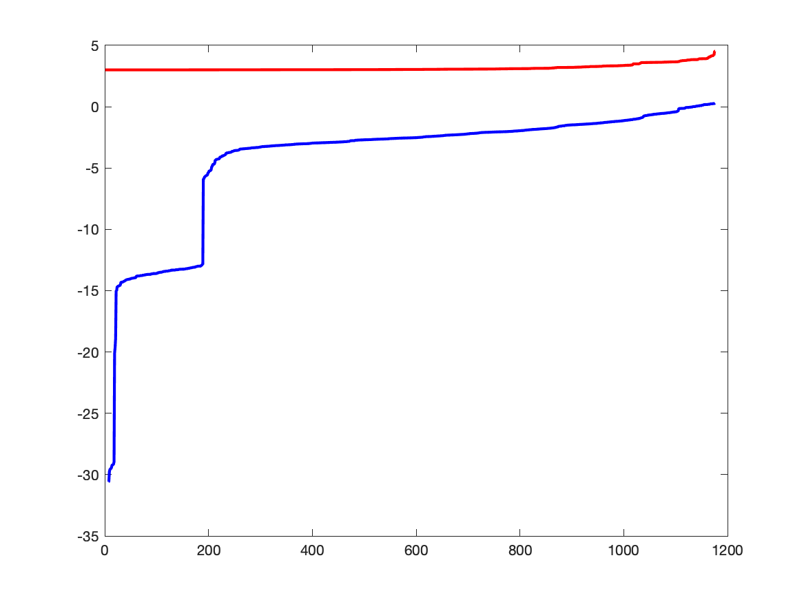
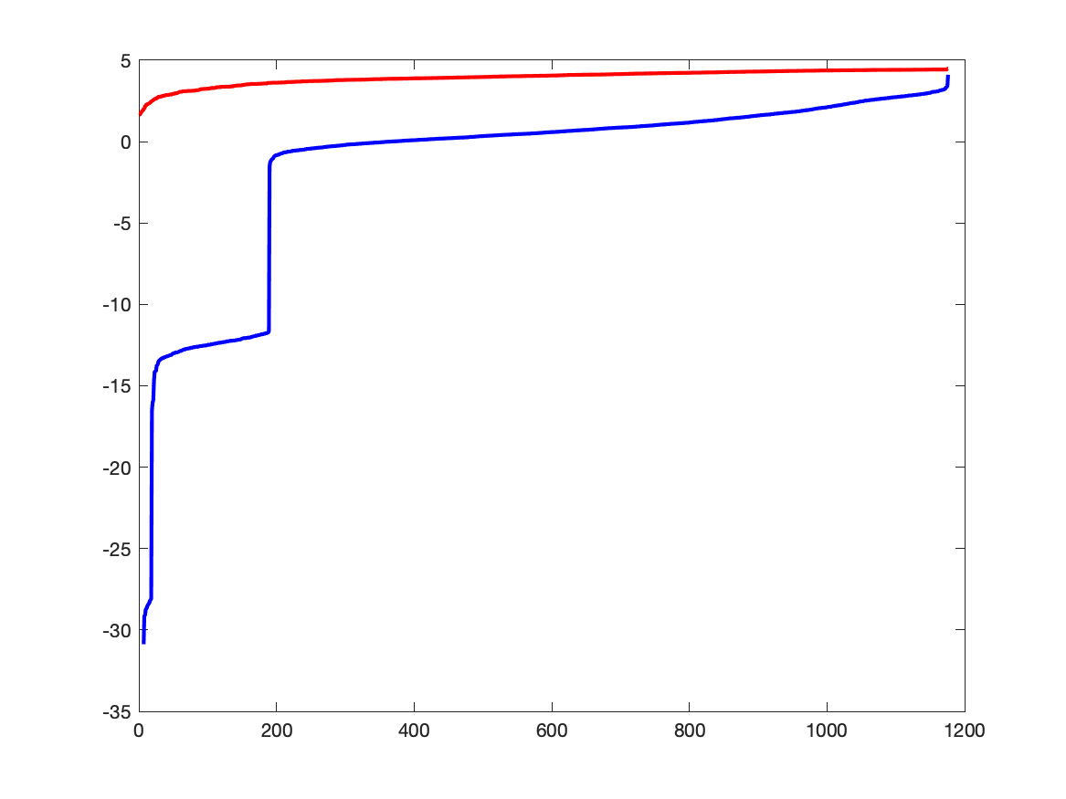
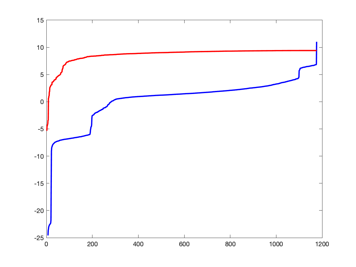
Figure 1: Problem tru7e; eigenvalues of $D^{\top}X_{\text{lin}}S_{\text{lin}}^{-1}D$ (red) and $\sum_{i=1}^{p}{\bf A}_{i}^{\top}(W_{i}^{0}\otimes W_{i}^{0}){\bf A}_{i}+\tilde{V}\tilde{V}^{\top}$ (blue) in iteration 2, 17 and 30 (left to right).

This observation lead to the idea of a simplified preconditioner called $H_{\beta}$ and defined as follows

(53) $$H_{\beta}=\sum_{i=1}^{p}\tau_{i}^{2}I+D^{\top}X_{\text{lin}}S_{\text{lin}}^{-1}D,$$

in which $\tau_{i}$ is defined as in the previous section. This matrix is easy to invert by 2.3; in fact, the matrix is diagonal in problems in Section 7. It is therefore an extremely “cheap” preconditioner that is efficient in the first iterations of the IP algorithm.

5.4 Preconditioner used in augmented Lagrangian approach

As has been shown previously in Section 3, see Eq. 14 and Eq. 29, the system matrix in the Newton systems in both, the purely primal and the primal-dual approach, is computed by the formula

(54) $$H=2\sum_{i=1}^{p}{\bf A}^{\!\!\top}_{i}(W_{i}\otimes V_{i}){\bf A}_{i}+H_{\rm{lin}},$$

where

(55) $$H_{\rm{lin}}: =rI+D^{\top}\bar{W}^{\rm{lin}}\left(y,X_{i}^{\rm{lin}},\pi^{\rm{lin}}\right)D,$$

(56) $$W_{i}: =\frac{1}{\pi^{\rm{lmi}}}\bar{X}_{i}(y)=\pi^{\rm{lmi}}\mathcal{Z}_{i}(y)X_{i}^{\rm{lmi}}\mathcal{Z}_{i}(y),$$

(57) $$V_{i}: =\pi^{\rm{lmi}}\mathcal{Z}_{i}(y)=-\pi^{\rm{lmi}}\left(A_{i}^{\rm{lmi}}(y)-\pi^{\rm{lmi}}I_{i}\right)^{-1}.$$

Here the lower index $i$ indicates the $i$-th LMI constraint and $A_{i}^{\rm{lmi}}:\mathbb{R}^{n}\to\mathbb{S}^{m_{i}},y\mapsto\sum_{j=1}^{n}y_{j}A_{i}^{(j)}-C_{i}$. Moreover, $y$ is the current primal iterate, $X_{i}\in\mathbb{S}^{m_{i}}$, $i=1,\ldots,p$, are the matrix multipliers from the current outer iteration, $\pi^{\rm{lmi}},\pi^{\rm{lin}}$ are the current penalty parameters and $\bar{W}^{\rm{lin}}\left(y,X_{i}^{\rm{lin}},\pi^{\rm{lin}}\right)$ is the diagonal matrix function defined in Eq. 15.

As the matrices $W_{i}$, $i=1,\ldots,p$, are scaled versions of the matrix multipliers, the low rank 2.5 directly applies to those. In addition, the eigenvalue structure of the matrices $V_{i}$, $i=1,\ldots,p$, is characterized by the following lemma.

Lemma 5.13.

1. Let $y\in\mathbb{R}^{n}$ be feasible with respect to all matrix inequalities. Then $0<\lambda_{j}(V_{i})\leq 1$ for all $j=1,\ldots,m_{i}$ and all $i=1,\ldots,p$.

2. If strict complementarity holds in a primal solution $y^{*}$ with associated matrix multipliers $X^{*}_{1},\ldots,X^{*}_{p}$ and the penalty parameter $\pi^{\rm{lmi}}$ is chosen sufficiently small, then the number of outlying eigenvalues of $V_{i}$ is (in a neighbourhood of the solution $y^{*}$) given by the rank $k_{i}$ of the corresponding multiplier matrix $X_{i}^{*}$ for all $i=1,\ldots,p$.

Proof 5.14.

1. Writing $V_{i}$ as a primary matrix function, we observe that the eigenvalues of every $A_{i}^{\rm{lmi}}(y)$ are transformed by the nonlinear function $\psi:\mathbb{R}\to\mathbb{R},t\to-\pi^{\rm{lmi}}/(t-\pi^{\rm{lmi}})$. Assuming that $y$ is feasible with respect to all matrix constraints, we have that all eigenvalues are non-positive. Now, taking the monotonicity of $\psi$, $\psi\geq 0$ on $(-\infty,\pi^{\rm{lmi}})$, $\psi(t)\to 0$ for $t\to-\infty$ and $\psi(0)=1$ into account, we see that $0<\lambda_{j}(V_{i})\leq 1$ for all $j=1,\ldots,m_{i}$ and all $i=1,\ldots,p$.

2. Let $\lambda_{i}^{1}\leq\ldots\leq\lambda_{i}^{m_{i}-k_{i}}<\lambda_{i}^{m_{i}-k_{i}+1}=\lambda_{i}^{m_{i}-k_{i}+2}=\ldots=\lambda_{i}^{m_{i}}=0$ denote the eigenvalues of $A_{i}^{\rm{lmi}}(y^{*})$ where $k_{i}$ denotes the rank of the associated multiplier matrix $X^{*}_{i}$. By, assumption $\pi^{\rm{lmi}}$ is sufficiently small, so we have that $\lambda_{i}^{1}\leq\ldots\leq\lambda_{i}^{m_{i}-k_{i}}\ll-\pi^{\rm{lmi}}<0$ and $0<-\pi^{\rm{lmi}}/\lambda_{i}^{m_{i}-k_{i}}\ll 1$. Finally, by the nonlinear transformation $\psi$ of the eigenvalues of $V_{i}$, we see that $0<\psi(\lambda_{i}^{j})\ll 1$ for all $j=1,\ldots,m_{i}-k_{i}$ and $\psi(\lambda_{i}^{j})=1$ for all $j=m_{i}-k_{i}+1,\ldots,m_{i}$ and all $i=1,\ldots,p$.

Lemma 5.13 suggests how to construct preconditioners for two different situations: in the first situation, we assume for a given LMI with index $i$ that only the matrix $W_{i}$ has a distinct eigenvalue structure, while for $V_{i}$ we just assume that the eigenvalues are essentially bounded between $0$ and $1$. In the second situation, we have that both matrices $V_{i}$ and $W_{i}$ exhibit the same eigenvalue structure. We note that this is somehow similar to the situation in the interior-point setting; however there, the matrices $V_{i}$ and $W_{i}$ would be the same.

We would like to note that in the numerical examples presented in Section 7, we will be always in the first situation, which means that the eigenvalues of $V_{i}$ will never be clearly separated from $1$. Nevertheless, we would like to demonstrate in the following how to construct efficient preconditioners for both situations.

For this, we can use the same idea as has been presented for the preconditioner $H_{\alpha}$ in Section 5.2. The first step is to decompose the matrix $H$ in Eq. 54. We introduce the following decompositions for $V_{i}$ and $W_{i}$, $i=1,\ldots,p$, which separate small from outlying eigenvalues precisely in the same way as in Eq. 46:

(58) $$V_{i} =V_{i}^{0}+\tilde{V_{i}}\tilde{V_{i}}^{\top},$$

(59) $$W_{i} =W_{i}^{0}+\tilde{W_{i}}\tilde{W_{i}}^{\top}.$$

Based on this we can formulate the following auxiliary results:

Lemma 5.15.

$H$ can be written as

(60) $$H=H_{\rm{lin}}+H^{0}_{\gamma}+H^{\rm{lr}}_{\gamma},$$

where

$$H^{0}_{\gamma} =2\sum_{i=1}^{p}{\bf A}^{\!\!\top}_{i}(W_{i}^{0}\otimes V_{i}){\bf A}_{i},$$

$$H^{\rm{lr}}_{\gamma} =2\sum_{i=1}^{p}{\bf A}^{\!\!\top}_{i}(\tilde{W}_{i}\otimes\Delta_{i})(\tilde{W}_{i}\otimes\Delta_{i})^{\top}{\bf A}_{i},$$

and $\Delta_{i}$ is chosen such that $V_{i}=\Delta_{i}\Delta_{i}^{\top}$ for all $i=1,\ldots,p$.

Proof 5.16.

It holds that

$$\begin{split}H&=H_{\rm{lin}}+2\sum_{i=1}^{p}{\bf A}^{\!\!\top}_{i}(W_{i}\otimes V_{i}){\bf A}_{i},\\ &=H_{\rm{lin}}+2\sum_{i=1}^{p}{\bf A}^{\!\!\top}_{i}(W_{i}^{0}\otimes V_{i}){\bf A}_{i}+2\sum_{i=1}^{p}{\bf A}^{\!\!\top}_{i}(\tilde{W}_{i}\tilde{W}_{i}^{\top}\otimes V_{i}){\bf A}_{i},\\ &=H_{\rm{lin}}+2\sum_{i=1}^{p}{\bf A}^{\!\!\top}_{i}(W_{i}^{0}\otimes V_{i}){\bf A}_{i}+2\sum_{i=1}^{p}{\bf A}^{\!\!\top}_{i}(\tilde{W}_{i}\tilde{W}_{i}^{\top}\otimes\Delta_{i}\Delta_{i}^{\top}){\bf A}_{i}\,.\end{split}$$

Now, Eq. 60 follows using standard properties of the Kronecker product.

Lemma 5.17.

$H$ can be written as

(61) $$H=H_{\rm{lin}}+H^{0}_{\delta}+H^{\rm{lr}}_{\delta},$$

where

$$H^{0}_{\delta} =2\sum_{i=1}^{p}{\bf A}^{\!\!\top}_{i}(W_{i}^{0}\otimes V_{i}^{0}){\bf A}_{i},$$

$$H^{\rm{lr}}_{\delta} =2\sum_{i=1}^{p}{\bf A}^{\!\!\top}_{i}\left((\tilde{W}_{i}\otimes\Theta_{i})(\tilde{W}_{i}\otimes\Theta_{i})^{\top}+(\tilde{V}_{i}\otimes\Gamma_{i})(\tilde{V}_{i}\otimes\Gamma_{i})^{\top}\right){\bf A}_{i}\,,$$

and the matrices $\Gamma_{i}$ and $\Theta_{i}$ are chosen such that $\Gamma_{i}\Gamma_{i}^{\top}=W_{i}^{0}+\frac{1}{2}\tilde{W}_{i}\tilde{W}_{i}^{\top}$ and $\Theta_{i}\Theta_{i}^{\top}=V_{i}^{0}+\frac{1}{2}\tilde{V}_{i}\tilde{V}_{i}^{\top}$ for all $i=1,\ldots,p$.

Proof 5.18.

Using Eq. 58 and Eq. 59 and the definitions of $\Gamma_{i},\Theta_{i}$, $i=1,\ldots,p$, we see:

$$\begin{split}H&=H_{\rm{lin}}+2\sum_{i=1}^{p}{\bf A}^{\!\!\top}_{i}(W_{i}\otimes V_{i}){\bf A}_{i},\\ &=H_{\rm{lin}}+2\sum_{i=1}^{p}{\bf A}^{\!\!\top}_{i}\left((W_{i}^{0}+\tilde{W}_{i}\tilde{W}_{i}^{\top})\otimes(V_{i}^{0}+\tilde{V}_{i}\tilde{V}_{i}^{\top})\right){\bf A}_{i}\\ &=H_{\rm{lin}}+2\sum_{i=1}^{p}{\bf A}^{\!\!\top}_{i}(W_{i}^{0}\otimes V_{i}^{0}){\bf A}_{i}\\ &\qquad+2\sum_{i=1}^{p}{\bf A}^{\!\!\top}_{i}\left((V_{i}^{0}+\frac{1}{2}\tilde{V}_{i}\tilde{V}_{i}^{\top})\otimes\tilde{W}_{i}\tilde{W}_{i}^{\top}+(W_{i}^{0}+\frac{1}{2}\tilde{W}_{i}\tilde{W}_{i}^{\top})\otimes\tilde{V}_{i}\tilde{V}_{i}^{\top}\right){\bf A}_{i}\\ &=H_{\rm{lin}}+2\sum_{i=1}^{p}{\bf A}^{\!\!\top}_{i}(W_{i}^{0}\otimes V_{i}^{0}){\bf A}_{i}\\ &\qquad+2\sum_{i=1}^{p}{\bf A}^{\!\!\top}_{i}\left(\tilde{W}_{i}\tilde{W}_{i}^{\top}\otimes\Theta_{i}\Theta_{i}^{\top}+\tilde{V}_{i}\tilde{V}_{i}^{\top}\otimes\Gamma_{i}\Gamma_{i}^{\top}\right){\bf A}_{i}\,.\end{split}$$

Now, again, Eq. 61 follows using standard properties of the Kronecker product.

Finally, efficient preconditioners can be built on the basis of the decompositions Eq. 60 and Eq. 61 by approximating the $H^{0}_{\delta}$ and $H^{0}_{\gamma}$ -terms as follows:

$$\begin{split}H_{\gamma}&=H_{\rm{lin}}+\sum_{i=1}^{p}\tau_{i}^{(1)}\tau_{i}^{(2)}{\rm diag}\left({\bf A}_{i}{\bf A}^{\!\!\top}_{i}\right)+H^{\rm{lr}}_{\delta},\\ H_{\delta}&=H_{\rm{lin}}+\sum_{i=1}^{p}\tau_{i}^{(1)}\tau_{i}^{(2)}{\rm diag}\left({\bf A}_{i}{\bf A}^{\!\!\top}_{i}\right)+H^{\rm{lr}}_{\gamma}.\end{split}$$

Here, for all $i=1,\ldots,p$, we choose $\tau_{i}^{(1)}$ to be the smallest eigenvalue of $W_{i}^{0}$ multiplied by 10 and $\tau_{i}^{(2)}$ to be the average of the eigenvalues of $V_{i}^{0}$ or $V_{i}$, respectively. The expression ${\rm diag}\left({\bf A}_{i}{\bf A}^{\!\!\top}_{i}\right)$ denotes a diagonal matrix of size $m_{i}\times m_{i}$ computed from ${\bf A}_{i}{\bf A}^{\!\!\top}_{i}$.

We finally note that the terms $H_{\rm{lin}}$ and $H^{\rm{lr}}_{\gamma}$, $H^{\rm{lr}}_{\delta}$ can be treated using the SMW-formula exactly as has been demonstrated in Eq. 51. Moreover, thanks to Lemma 5.15 and Lemma 5.17, Theorem 5.1 applies to the preconditioners presented above and also the complexity formulas are the same as presented for $H_{\alpha}$ preconditioner due to their analogous construction.

6 Application: truss topology optimization

6.1 Truss notation

The notation used throughout Section 6 is specific for this application and unrelated to the rest of the paper.

By truss we understand a mechanical structure, an assemblage of pin-jointed uniform straight bars made of elastic material, such as steel or aluminium. The bars can only carry axial tension and compression. We denote by $m$ the number of bars and by $N$ the number of joints. The positions of the joints are collected in a vector $y$ of dimension $\mathop{{\widetilde{n}}}:=dim\cdot N$ where $dim$ is the spatial dimension of the truss. The material properties of bars are characterized by their Young’s moduli $E_{i}$, the bar lengths are denoted by $\ell_{i}$ and bar volumes by $t_{i}$, $i=1,\ldots,m$.

For an $i$-th bar, let $\gamma_{i}$ be the vector of directional cosines; e.g., for $dim=2$, we define

$$\gamma_{i}={\frac{1}{\ell_{i}}}\left(-(y_{1}^{(k)}-y_{1}^{(j)}),\quad-(y_{2}^{(k)}-y_{2}^{(j)}),\quad y_{1}^{(k)}-y_{1}^{(j)},\quad y_{2}^{(k)}-y_{2}^{(j)}\right)^{\top},$$

where $y^{(j)}$ and $y^{(k)}$ are the end-points of the bar.

Let $f\in\mathbb{R}^{\mathop{{\widetilde{n}}}}$ be a load vector of nodal forces. The response of the truss to the load $f$ is measured by nodal displacements collected in a displacement vector $u\in\mathbb{R}^{\mathop{{\widetilde{n}}}}$. Some of the displacement components may be restricted: a node can be fixed in a wall, then the corresponding displacements are prescribed to be zero. The number of free nodes multiplied by the spatial dimension will be denoted by $n$ and we will assume that $f\in\mathbb{R}^{n}$ and $u\in\mathbb{R}^{n}$.

We introduce the bar stiffness matrices $K_{i}$ and assemble them in the global stiffness matrix of the truss

(62) $$K(t)=\sum_{i=1}^{m}t_{i}K_{i}=\sum_{i=1}^{m}t_{i}\frac{E_{i}}{\ell_{i}^{2}}\gamma_{i}\gamma_{i}^{\top},\quad i=1,\ldots,m$$

and introduce the equilibrium equation

(63) $$K(t)u=f\,.$$

Assumption 6.1.

$K(\mathbf{1})$ with $\mathbf{1}=(1,1,\ldots,1)\in\mathbb{R}^{m}$ is positive definite and the load vector $f$ is in the range space of $K(\mathbf{1})$.

6.2 Truss topology problem, rank of the solution

Let $0\leq\underline{t}_{i}\leq\overline{t}_{i},\ i=1,\ldots,m$ and $\gamma$ be a positive constant. The basic truss topology problem reads as follows.

(64) $$\min_{t\in\mathbb{R}^{m},u\in\mathbb{R}^{n}}\sum_{i=1}^{m}t_{i}$$

subject to

$$\qquad K(t)u=f$$

$$\qquad f^{\top}u\leq\gamma$$

$$\qquad\underline{t}_{i}\leq t_{i}\leq\overline{t}_{i},\quad i=1,\ldots,m\,.$$

The following version of the Schur complement theorem can be found, e.g., in [3].

Lemma 6.1.

Let $t\in\mathbb{R}^{m}$, $t\geq 0$, and $\gamma\in\mathbb{R}$ be fixed. Then there exists $u\in\mathbb{R}^{n}$ satisfying

$$K(t)u=f\qquad\mbox{and}\qquad f^{\top}u\leq\gamma$$

if and only if

$$\begin{pmatrix}\gamma&-f^{\top}\\ -f&K(t)\end{pmatrix}\succeq 0\,.$$

From the above lemma, we immediately get an equivalent SDP formulation of the problem:

(65) $$\min_{t\in\mathbb{R}^{m}}\sum_{i=1}^{m}t_{i}$$

subject to

$$\qquad\begin{pmatrix}\gamma&-f^{\top}\\ -f&K(t)\end{pmatrix}\succcurlyeq 0$$

$$\qquad\underline{t}_{i}\leq t_{i}\leq\overline{t}_{i},\quad i=1,\ldots,m\,.$$

The dual to Eq. 65 reads as follows.

(66) $$\max_{\stackrel{{\scriptstyle\scriptstyle X\in\mathbb{S}^{n+1}}}{{\overline{\rho}\in\mathbb{R}^{m},\underline{\rho}\in\mathbb{R}^{m}}}}\begin{pmatrix}-\gamma&f^{\top}\\ f&0\end{pmatrix}\bullet X-\sum_{i=1}^{m}\overline{\rho}_{i}\overline{t}_{i}+\sum_{i=1}^{m}\underline{\rho}_{i}\underline{t}_{i}$$

subject to

$$\qquad\begin{pmatrix}0&0\\ 0&K_{i}\end{pmatrix}\bullet X-\overline{\rho}_{i}+\underline{\rho}_{i}=1,\quad i=1,\ldots,m$$

$$\qquad X\succcurlyeq 0$$

$$\qquad\overline{\rho}_{i}\geq 0,\ \underline{\rho}_{i}\geq 0,\quad i=1,\ldots,m\,.$$

Lemma 6.2.

Problems Eq. 65, Eq. 66 satisfy 2.2 and 2.3.

Proof 6.3.

Every vector $\gamma_{i}$ in Eq. 62 has at most 4 non-zero elements (6 in 3D space) and thus every matrix $K_{i}$ has at most 16 (36) non-zero elements, independently of the size of the problem; hence 2.2 is satisfied. 2.3 is trivially satisfied for box constraints on $t_{i}$.

Proposition 6.4.

[1, Chap. 2.5] Let $t^{*}\in\mathbb{R}^{m}$ be a solution of the minimum volume problem Eq. 64 with $\underline{t}_{i}=0$, $i=1,\ldots,m$. There exists a sequence $\{t_{k}\}_{k=1}^{\infty}$, $t_{k}\in\mathbb{R}^{m}$, with the following properties

• $t_{k}$ is a solution of Eq. 64 with $\underline{t}_{i}=\varepsilon_{k}$, $i=1,\ldots,m$  and $\varepsilon_{k}\to 0$ as $k\to\infty$ ;

• $t_{k}\to t^{*}$ as $k\to\infty$ .

Theorem 6.5.

There exists a solution $(X^{*},\overline{\rho}^{*},\underline{\rho}^{*})\in\mathbb{S}^{n+1}\times\mathbb{R}^{m}\times\mathbb{R}^{m}$ of the dual SDP problem Eq. 66 such that the rank of $X^{*}$ is one.

Proof 6.6.

Let $t^{*}$ be a solution of the primal SDP problem Eq. 65 associated with Eq. 66. Denote by $S^{*}\in\mathbb{S}^{n+1}$ the primal slack matrix variable

$$S^{*}=\begin{pmatrix}\gamma&-f^{\top}\\ -f&K(t^{*})\end{pmatrix}\,.$$

This matrix is complementary to any solution $X$ of the dual SDP problem, i.e.,

$$\langle X,S^{*}\rangle=0\,.$$

As $X$ and $S^{*}$ are commuting and thus simultaneously diagonalizable, we have the following rank condition (see, e.g., [12]):

(67) $$\operatorname{rank}(S^{*})+\operatorname{rank}(X)\leq n+1\,.$$

If $\underline{t}_{i}>0$, $i=1,\ldots,m$, the matrix $K(t^{*})$ is positive definite and, due to 6.1, has a full rank $n$. Hence, by the above rank condition, the rank of any dual solution $X$ is at most one. Since we exclude trivial solutions with $X\equiv 0$, the rank of $X$ is exactly equal to one.

Assume now that $\underline{t}_{i}=0$, $i=1,\ldots,m$, i.e., the matrix $K(t^{*})$ can be rank deficient. Due to Proposition 6.4, there is a sequence of solutions $\{S_{k}\}$ to the problem Eq. 65 with $(\underline{t}_{i})_{k}=\varepsilon_{k}$, $\varepsilon_{k}\to 0$ as $k\to\infty$, such that $S_{k}\to S^{*}$. Associated with $\{S_{k}\}$ there is a sequence of dual solutions $\{X_{k}\}$, such that any pair $(S_{k},X_{k})$ satisfies the complementarity condition and thus the rank condition. By this construction, the matrices $K(t_{k})$ are strictly positive definite and thus, due to 6.1, have full rank $n$. From the rank condition Eq. 67 it follows that the rank of $X_{k}$ is at most one and thus exactly equal to one. Hence there is a sequence of vectors $\{x_{k}\}$ such that $X_{k}=x_{k}x_{k}^{\top}$ for each $k$. Then $X^{*}=x^{*}(x^{*})^{\top}$ is a solution of the dual SDP problem and thus complementary to $S^{*}$. By construction, $X^{*}$ is a rank-one matrix.

Corollary 6.7.

Let $\underline{t}_{i}>0$ for $i=1,\ldots,m$. Then the solution $X^{*}\in\mathbb{S}^{n+1}$ of the dual SDP problem Eq. 66 has rank one.

Problems with approximate low rank

The conclusion of Corollary 6.7 changes when we assume that $\underline{t}_{i}=0$ for $i=1,\ldots,m$. In this case, some bars may “vanish" at the optimum (the corresponding $t_{i}=0$). Moreover, some nodes of the structure may only be connected by these vanishing bars and hence also “vanish" from the optimal structure. As a consequence, the stiffness matrix $K(t)$ will become singular with as many zero eigenvalues as the vanished nodes (not connected to the optimal structure). Then

$$\operatorname{rank}(S^{*})<n\quad\mbox{and thus}\quad\operatorname{rank}(X^{*})>1\quad\mbox{is possible}\,.$$

Hence, while there is always a rank-one solution by Theorem 6.5, in this case there might be other solutions with higher rank. In particular, when we solve the problems by an interior point method, the pair of solutions $(S^{*},X^{*})$ will be maximally complementary ([12, Thm. 3.4]), so the rank of $X^{*}$ will be equal to the number of the vanished nodes plus one.

Example 6.1.

Figure 2 shows an example of a truss with potentially six nodes (the remaining three nodes are fixed by boundary conditions); at the optimum, nodes 1, 2, 3, 4, 6 vanished—they are not connected to the optimal structure but are still present in the problem and its stiffness matrix. Hence the solution of the dual problem may have rank of up to $(1+2\times 5)=11$.

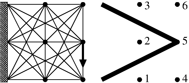
Figure 2: A problem with five nodes vanishing at the optimum; initial structure (left) and optimal solution (right).

The associated Table 1 presents, column-wise, eigenvalues of $X^{*}$ and $S^{*}$ for $\underline{t}>0$ (when rank-one solution $X^{*}$ is expected) and eigenvalues of $X^{*}$ and $S^{*}$ for $\underline{t}=0$ (when one outlying eigenvalue of $X^{*}$ is expected).

Table 1: Eigenvalues of $X^{*}$ and $S^{*}$ for problem in Fig. 2.

$\lambda(X^{*}),\ \underline{t}>0$

1.980482521248879
0.000000102260913
0.000000086085241
0.000000068216515
0.000000054110869
0.000000042818584
0.000000039334355
0.000000033270286
0.000000032811718
0.000000028005339
0.000000027431494
0.000000000001029
0.000000000000041

$\lambda(S^{*}),\ \underline{t}>0$

0.000000000000102
0.000003116874928
0.000003956920433
0.000006409263345
0.000007529457678
0.000009477992158
0.000011708852890
0.000012193659241
0.000014115281046
0.000014761068984
0.000016565957597
0.399999306252456
10.10000007997102

$\lambda(X^{*}),\ \underline{t}=0$

2.064483254260574
0.010238711360358
0.009214785863400
0.005367091514209
0.005013654697043
0.003545367975067
0.002923233469802
0.002610639717586
0.001846306250799
0.001771660792931
0.001555022631457
0.000000000000031
0.000000000000001

$\lambda(S^{*}),\ \underline{t}=0$

0.000000000010001
0.000000000013521
0.000000000013687
0.000000000016235
0.000000000017372
0.000000000018683
0.000000000020485
0.000000000021874
0.000000000024806
0.000000000028448
0.000000000032822
0.400000000006957
10.10000000001012

Notice that the number of the vanished nodes depends on the initial setting of the problem and can be rather high, as compared to the total number of the nodes.

6.3 Truss topology problem, vibration constraints

Formulation of the basic truss topology problem Eq. 64 as an SDP is rather academic. It was shown, e.g., in [16] that a dual to Eq. 64 is a convex nonlinear programming problem that can be solved very efficiently by interior point methods. The SDP formulation gains significance once we add more, important and practical, constraints to the problem. In particular, it was shown in [2, 3] that a constraint on natural (free) vibrations of the optimal structure leads to a linear matrix inequality and that this is, arguably, the best way how to treat this constraint.

The free vibrations are the squares of the eigenvalues of the following generalized eigenvalue problem

(68) $$K(t)w=\lambda\left(M(t)+M_{0}\right)w\,.$$

Here $M(t)=\sum\limits_{i=1}^{m}t_{i}M_{i}$ is the so-called mass matrix that collects information about the mass distribution in the truss. The matrices $M_{i}$ are positive semidefinite and have the same sparsity structure as $K_{i}$. The non-structural mass matrix $M_{0}$ is a constant, typically diagonal matrix with very few nonzero elements.

Low vibrations are dangerous and may lead to structural collapse. Hence we typically require the smallest free vibration to be bigger than some threshold, that is:

$$\lambda_{\min}\geq\overline{\lambda}\quad\mbox{for a given}\ \overline{\lambda}>0\,\$$

where $\lambda_{\min}$ is the smallest eigenvalue of the generalized eigenvalue problem Eq. 68. This constraint can be equivalently written as a linear matrix inequality

(69) $$K(t)-\overline{\lambda}\left(M(t)+M_{0}\right)\succcurlyeq 0$$

which is to be added to the basic truss topology problem. As Eq. 69 is a linear matrix inequality in variable $t$, it is natural to add this constraint to the primal SDP formulation Eq. 65. We will thus get the following linear SDP formulation of the truss topology design with a vibration constraint:

(70) $$\min_{t\in\mathbb{R}^{m}}\sum_{i=1}^{m}t_{i}$$

subject to

$$\qquad\begin{pmatrix}\gamma&-f^{\top}\\ -f&K(t)\end{pmatrix}\succcurlyeq 0$$

$$\qquad K(t)-\overline{\lambda}\left(M(t)+M_{0}\right)\succcurlyeq 0$$

$$\qquad\underline{t}_{i}\leq t_{i}\leq\overline{t}_{i},\quad i=1,\ldots,m\,.$$

It has been shown, e.g., in [35] that, when $\underline{t}_{i}>0$, the rank of the optimal dual variable to the second matrix inequality is equal to the multiplicity of the smallest eigenvalue of Eq. 68. This multiplicity depends on the geometry of the optimal structure but is, typically very low, usually not bigger than 1 or 2. Thus the new problem Eq. 69 fits in our framework of SDPs with very low rank dual solutions.

7 Numerical experiments

7.1 Problem database

To test our algorithms, we generated a library of truss topology problems of various sizes, both with and without the vibration constraint. All problems have the same geometry, boundary conditions and loads and only differ in the number of potential nodes and bars.

The geometry and loading for TTO without vibration (formulation Eq. 65) is as in Fig. 2-left, while the data for problems with the vibration constraint (formulation Eq. 70) differ only in the horizontal orientation of the load vector. We have generated four groups of problems with the following naming convention. In each group, all nodes in the initial ground structure are connected by potential bars.

standard TTO problem Eq. 65 with $\underline{t}=0$, discretized by $n\times n$ nodes;

standard TTO problem Eq. 65 with $\underline{t}=\varepsilon>0$, discretized by $n\times n$ nodes;

TTO problem with the vibration constraint Eq. 70 with $\underline{t}=0$, discretized by $n\times n$ nodes;

TTO problem with the vibration constraint Eq. 70 with $\underline{t}=\varepsilon>0$, discretized by $n\times n$ nodes.

Table 2 present dimensions of the generated problems. Notice that these problems satisfy 2.4.

Table 2: Problems tru<n> and tru<n>e and problems vib<n> and vib<n>e, number of variables $n$, size of the LMI constraint $m$ and number of linear constraints.

problem	$n$	$m$	lin. constr.
tru3(e)	36	13	72
tru5(e)	300	41	600
tru7(e)	1176	85	2352
tru9(e)	3240	145	6480
tru11(e)	7260	221	14520
tru13(e)	14196	313	28392
tru15(e)	25200	421	50400
tru17(e)	41616	545	83232
tru19(e)	64980	685	129960
tru21(e)	97020	841	194040
tru23(e)	139656	1013	279312
tru25(e)	195000	1201	390000

problem	$n$	$m$	lin. constr.
vib3(e)	36	(13, 12)	72
vib5(e)	300	(41, 40)	600
vib7(e)	1176	(85, 84)	2352
vib9(e)	3240	(145, 144)	6480
vib11(e)	7260	(221, 220)	14520
vib13(e)	14196	(313, 312)	28392
vib15(e)	25200	(421, 420)	50400
vib17(e)	41616	(545, 544)	83232
vib19(e)	64980	(685, 684)	129960
vib21(e)	97020	(841, 840)	194040
vib23(e)	139656	(1013, 1012)	279312
vib25(e)	195000	(1201, 1200)	390000

For illustration, Fig. 3 shows optimal results for problems tru25 and vib19.

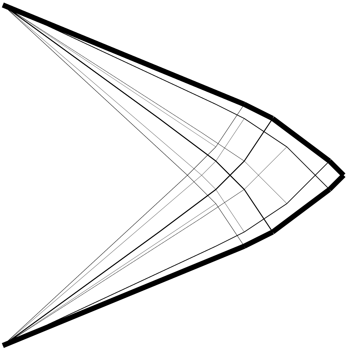
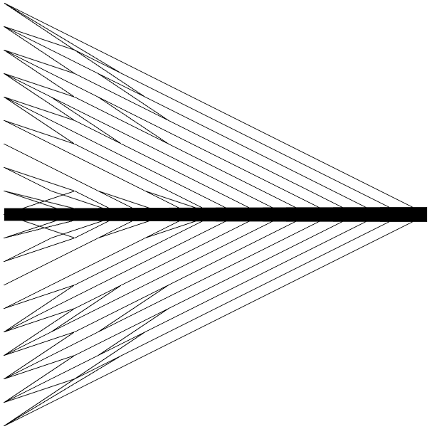
Figure 3: Optimal results for problems tru25 (left) and vib19 (right).

7.2 Numerical results

In this section we will present numerical results for the truss topology problems from the problem database. The two algorithms were implemented in MATLAB codes PDAL and Loraine (Low-rank interior-point). The codes use the same modules for data input and for the solution of the linear systems. Both codes use DIMACS stopping criteria [26] with $\varepsilon_{\scriptscriptstyle\rm DIMACS}=10^{-5}$.

In Table 3 we present the value of parameters chosen in PDAL (notice that they differ for the tru and vib collections). Moreover for the block constraints in the tru problems we are using the Penalty-Barrier function with $\tau=0.5$ while for the vib problems we use a pure barrier function. Loraine parameters have already been specified in Algorithm 4.

The stopping parameter for the CG method $\varepsilon_{\scriptscriptstyle\rm CG}$ in Algorithm 5 has been set and updated as follows: we start with $\varepsilon_{\scriptscriptstyle\rm CG}=0.01$ and multiply it after every major iteration by 0.5, until it reaches the value $10^{-6}$; then we continue with this value till convergence of the optimization algorithm.

Table 3: Parameters used in PDAL for the tru and vib problems

param	tru	vib	param	tru	vib
$\pi^{\rm{lin}}_{\rm{min}}$	$10^{-9}$	$10^{-11}$	$\gamma^{\rm{lin}}$	0.5	1
$\pi^{\rm{lmi}}_{\rm{min}}$	$10^{-5}$	$10^{-5}$	$\gamma^{\rm{lmi}}$	0.5	0.8
$\pi^{\rm{lin}}_{\rm{upd}}$	0.5	0.3	$r$	0.01	0.01
$\pi^{\rm{lmi}}_{\rm{upd}}$	0.5	0.3	$\varepsilon$	$10^{-6}$	$10^{-6}$

Unless stated otherwise, we use the following preconditioners:

PDAL:

The preconditioner $H_{\gamma}$ described in Section 5.4 is used throughout all iterations.

Loraine:

A hybrid preconditioner called $H_{\rm hyb}$: we start with $H_{\beta}$ Eq. 53 until the criterion below is satisfied and then switch to $H_{\alpha}$ Eq. 50:

$$N_{\rm cg\_iter}>kp\sqrt{n}/10\ \ \&\ \ N_{\rm iter}>\sqrt{n}/60\,.$$

Here $N_{\rm iter}$ is the current IP iteration and $N_{\rm cg\_iter}$ the number of CG steps needed to solve the corrector equation in this iteration. This criterion is, obviously, purely heuristic. We further choose the value of $\tau$ in $H_{\alpha}$ and $H_{\beta}$ as

$$\tau=\lambda_{1}(W_{i})+0.5\,{\rm mean}(\lambda_{1}(W_{i}),\ldots,\lambda_{m-k_{i}}(W_{i}))\,.$$

All problems were solved on an iMac with 3.6 GHz 8-Core Intel Core i9 and 40 GB 2667 MHz DDR4 using MATLAB R2020a.

Before presenting the results, we want to illustrate the efficiency of the used preconditioners, in particular, in the light of the assumption of Theorem 5.11.

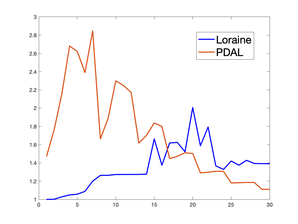
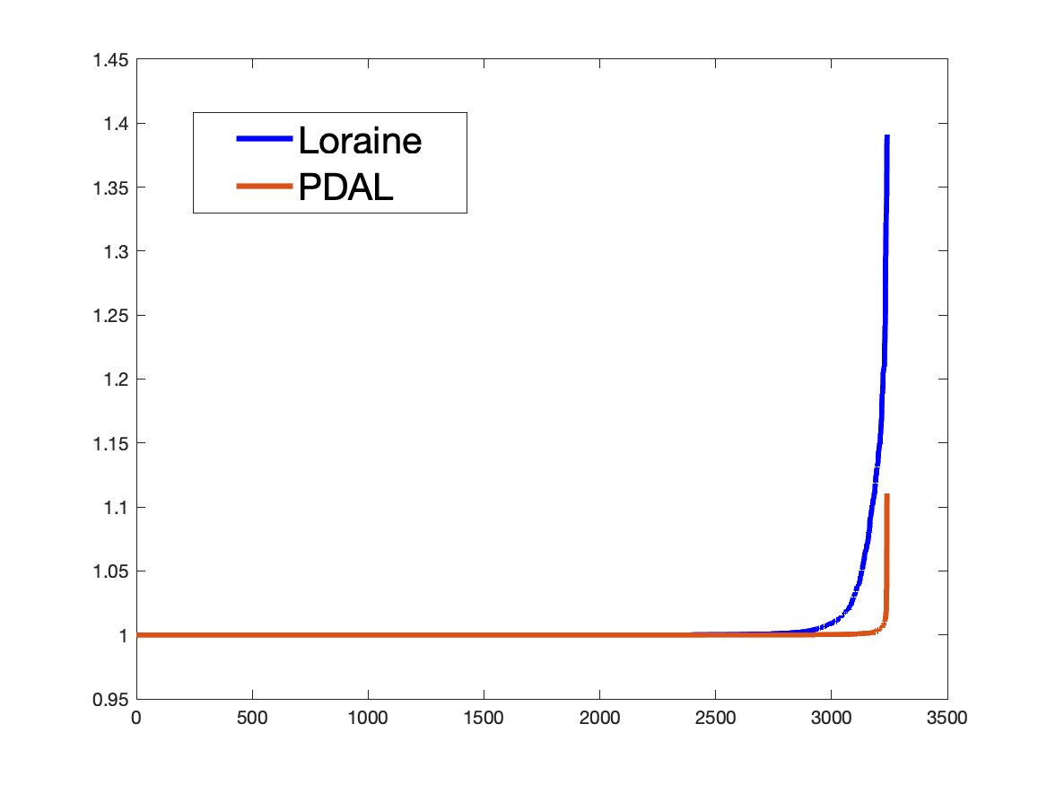
Figure 4: Left: The history of the last 30 condition numbers of the preconditioned matrix in Loraine (blue) and PDAL (red) in tru9 problem. Right: Eigenvalues of the preconditioned matrix in the last iteration of Loraine (blue) and PDAL (red).

In Fig. 4–left we present the history of the condition numbers of the preconditioned matrices for problem tru9; a complete history for Loraine and the last 30 iterations for PDAL. While the history differs for the two algorithms, the condition numbers are very low and, in case of PDAL, decrease when converging to the solution. For this problem, we also computed the values of $\underline{\varepsilon}$ and $\overline{\varepsilon}$ from Theorem 5.11 and found that the estimate of the condition number in this theorem was always sharp. Fig. 4–right depicts all eigenvalues of the preconditioned matrix in the last iteration. Most of the eigenvalues are very close or equal to one and the matrices have only a few outlying eigenvalues, albeit still not far from one.

We now present results for all tru and vib problems using Loraine and PDAL. These are shown in Tables 4 and 5. The tables present the number of iterations of the respective algorithm, the total number of CG iterations using the hybrid preconditioner $H_{\rm hyb}$ in case of Loraine and $H_{\alpha}$ in case of PDAL. This is followed by CPU time spent in the optimization solver and time per iteration. Notice that PDAL solves one linear system per iteration, while Loraine solves two (predictor and corrector). For all problems we set the expected rank of the dual solutions $k=1$.

Table 4: Loraine and PDAL in tru$*$ problems

	Loraine				PDAL
	iter	CG iter	CPU	CPU/iter	iter	CG iter	CPU	CPU/iter
tru3	16	122	0.01	0.00	35	107	0.04	0.00
tru5	21	190	0.08	0.00	61	357	0.28	0.00
tru7	27	236	0.24	0.01	62	310	0.54	0.01
tru9	31	333	0.65	0.02	69	374	1.5	0.02
tru11	36	370	1.6	0.04	78	435	3.4	0.04
tru13	45	500	4.5	0.10	102	818	10	0.10
tru15	52	882	11	0.22	97	670	20	0.21
tru17	53	980	24	0.45	96	744	39	0.41
tru19	64	1310	51	0.80	101	808	71	0.70
tru21	65	1325	84	1.29	111	965	151	1.36
tru23	72	2450	189	2.63	112	1019	270	2.41
tru25	87	2148	317	3.64	142	1929	634	4.46

Table 5: Loraine and PDAL in vib$*$ problems

	Loraine				PDAL
	iter	CG iter	CPU	CPU/iter	iter	CG iter	CPU	CPU/iter
vib3	20	209	0.04	0.00	66	251	0.2	0.00
vib5	31	411	0.21	0.01	69	434	0.45	0.01
vib7	39	501	0.67	0.02	69	372	0.91	0.01
vib9	47	663	2.2	0.05	82	473	3.0	0.04
vib11	59	995	6.1	0.10	99	464	7.6	0.08
vib13	69	1153	16	0.23	112	508	18	0.16
vib15	80	1480	37	0.46	131	534	44	0.34
vib17	94	1781	92	0.98	130	501	91	0.70
vib19	108	2116	189	1.75	145	536	177	1.22
vib21	120	2844	401	3.34	173	723	456	2.64
vib23	130	2720	718	5.52	193	799	961	4.98
vib25	143	3752	1321	9.24	205	808	1724	8.41

The following Figs. 5, 6, 7 and 8 depict graphs of CPU times versus the number of variables for all four groups of problems, presented in the log-log scale. We can see that, while PDAL needs more iterations, the times per iteration are almost identical for the two codes. In particular, the time grows almost linearly (factor $\sim$1.25) with the size of the problem.

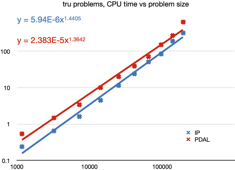
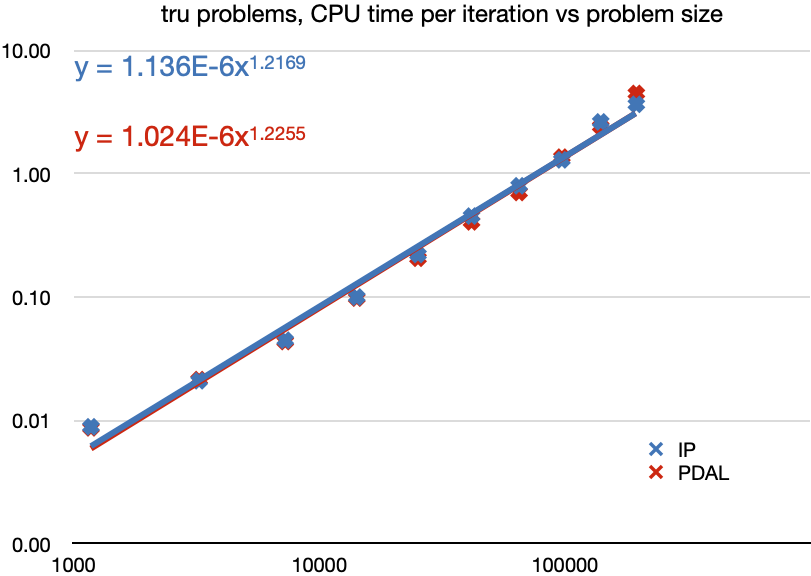
Figure 5: Loraine (blue) and PDAL (red) in tru$*$ problems. CPU time vs number of variables in log-log scale.

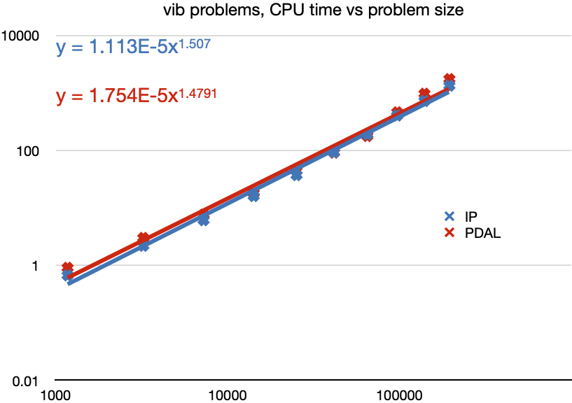
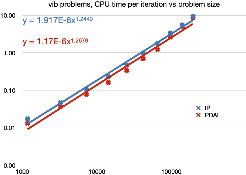
Figure 6: Loraine (blue) and PDAL (red) in vib$*$ problems. CPU time vs number of variables in log-log scale.

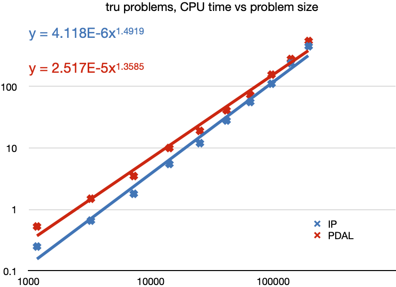
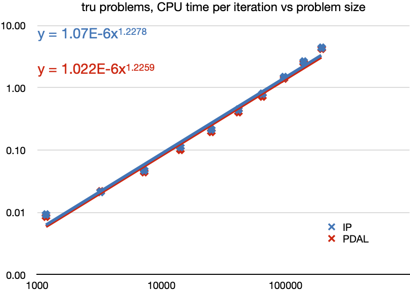
Figure 7: Loraine (blue) and PDAL (red) in tru$*$e problems. CPU time vs number of variables in log-log scale.

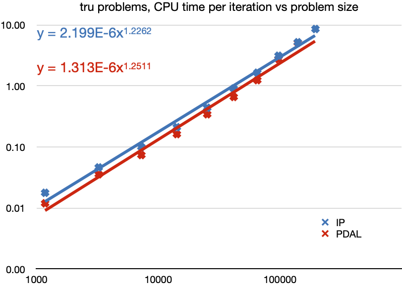
Figure 8: Loraine (blue) and PDAL (red) in vib$*$e problems. CPU time vs number of variables in log-log scale.

7.3 Other software

In this section we give a brief comparison Loraine and PDAL with other SDP software. First we present a comparison of Loraine, our IP implementation, with the solver MOSEK [27] that is also based on an interior-point algorithm. While this comparison may seem unfair, as MOSEK uses a direct solver to solve the linear systems, we believe that it gives a good perspective of the clear advantage of iterative solvers with good preconditioners, when available and when applicable. The results are presented in Table 6; we again give the number of iterations of the solver, CPU time and CPU time per one iteration. The table also shows the speed-up with respect to MOSEK and speed-up per iteration. We only present results for problems tru3–tru17; for the larger problems MOSEK exceeded the available 40GB RAM.

Table 6: Loraine and MOSEK in tru$*$ problems

	Mosek			Loraine
problem	iter	CPU	CPU/iter	iter	CG iter	CPU	CPU/iter	speed-up	s-up/iter
tru3	14	0.22	0.02	16	122	0.01	0.00	22	25
tru5	15	0.23	0.02	21	190	0.08	0.00	2.9	4.0
tru7	17	0.78	0.05	27	236	0.24	0.01	3.3	5.2
tru9	20	5.6	0.28	31	333	0.65	0.02	8.6	13
tru11	26	44	1.69	36	370	1.61	0.04	27	37
tru13	29	235	8.10	45	500	4.5	0.10	52	81
tru15	32	1079	33.72	52	882	11.5	0.22	93	152
tru17	37	4671	126.24	53	980	24	0.45	194	278

In Fig. 9 we give a comparison of the CPU time per iteration. While MOSEK actually exceeds the theoretical complexity with coefficient 2.2, the complexity of Loraine is almost linear for these problems.

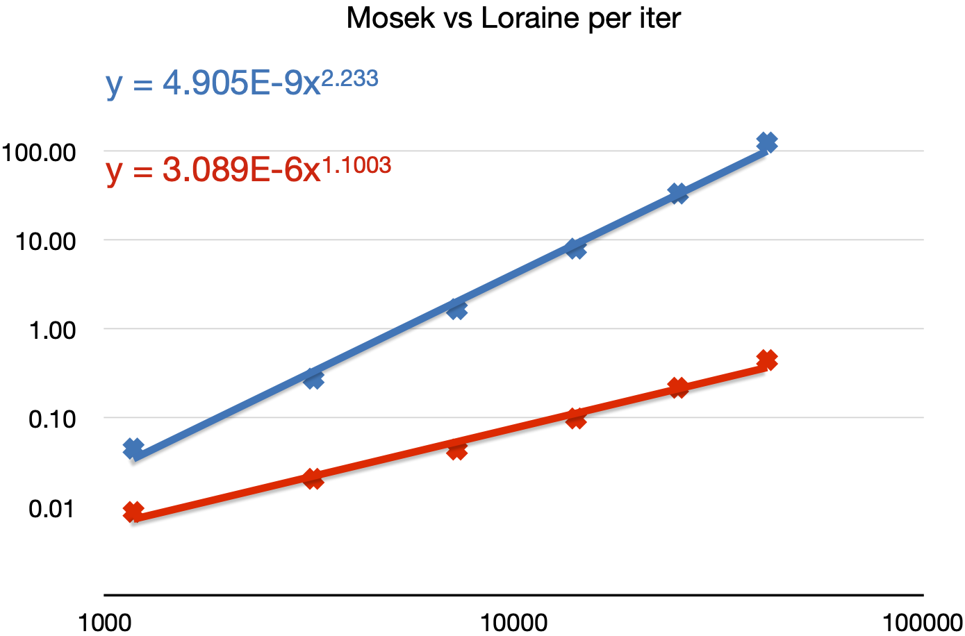
Figure 9: Loraine (red) and MOSEK (blue) in tru$*$ problems. CPU time per iteration vs number of variables in log-log scale.

The next Table 7 gives results of Loraine with the preconditioner ${H_{\alpha}}$ compared with other solvers that could potentially benefit from the low rank information: Loraine with the preconditioner $\widetilde{H}$ by Zhang and Lavaei [42]; SDPNAL+ [39], an implementation of semismooth Newton-CG augmented Lagrangian method; and SDPLR [10] using a nonlinear programming algorithm based on low-rank factorization of the variables. SDPNAL+ and SDPLR were used with default stopping tolerance. None of these codes can solves problems bigger than tru11 before reaching the maximum number of iterations, either internal or global. While Loraine solutions satisfy DIMACS criteria with $10^{-5}$, other codes often finish with lower precision, as documented by the final value of the objective function.

Table 7: Other solvers

	Loraine with ${H_{\alpha}}$			Loraine with $\widetilde{H}$			SDPNAL+		SDPLR
	iter	CG iter	CPU	iter	CG iter	CPU	iter	CPU	iter	CPU
tru3	16	122	0.01	16	131	0.02	440	0.5	15	0.01
tru5	21	190	0.08	21	197	0.3	9674	29	18	1.7
tru7	27	237	0.27	27	348	3.7	6324	55	19	21
tru9	31	331	0.94	31	570	42	47579	468	20	179
tru11	36	344	2.62	36	625	303	maxit		22	2469

7.4 No preconditioner

Recall the two contributing factors to the efficiency of the presented methods: a) the dedicated preconditioner and b) the very fact of using an iterative method for the solution of linear systems, a method requiring only matrix-vector multiplications, without the need to assemble and store the actual matrix. While our main focus was on the preconditioner, the second factor is just as important. Indeed, it turns out that for several problem classes, no preconditioner is actually needed; typically for the matrix completion problems used in [4, 42] or problems resulting form relaxation of combinatorial optimization problems. The typical feature of these problems is the lack of linear constraints and the fact that the matrix ${\bf A}^{\!\!\top}{\bf A}$ is diagonal. In such a case, our $H_{\alpha}$ is almost identical to $\widetilde{H}$ of [42].

For example, when solving problem gpp500-1 from SDPLIB [8] (solution of rank 6), Loraine needed 288 total CG steps (2 in the last IP iteration) and 96 seconds to solve the problem using $H_{\alpha}$ and 4045 CG steps (539 in the last IP iteration) and (only) 14 seconds to solve the problem without preconditioner. In another example, we solved the matrix completion problem ([4, 42]) with $n=36000$, $m=1200$ and $\operatorname{rank}X^{*}=1$; in this case Loraine needed 580 total CG steps and 53 seconds to solve the problem using $H_{\alpha}$ and 1108 CG steps and 48 seconds to solve the problem without preconditioner.

To demonstrate that this is not the case of the truss topology problems, we include Table 8. It presents results of Loraine with no preconditioner for problems that are still solvable before reaching the maximum number of CG iteration in one linear system, set to 100000. We clearly see the advantage of using the preconditioner; confront Tables 4 and 5.

Table 8: Loraine with no preconditioner

	iter	CG iter	CPU		iter	CG iter	CPU
tru3	16	346	0.01	vib3	21	3115	0.06
tru5	21	2385	0.15	vib5	31	46949	2.76
tru7	27	10091	0.97	vib7	40	166135	24.9
tru9	30	33163	7.3	vib9	48	432416	181
tru11	36	77700	45

8 Conclusions

We have introduced a preconditioner for the CG method that can be used in two different second-order algorithms for linear SDP. The preconditioner utilizes low rank of the SDP solutions. We have demonstrated that it is extremely efficient—as a preconditioner—for SDP problems arising from structural optimization.

How do the two optimization algorithms, PDAL and IP, compare? The interior-point algorithm needs, in general, less overall iterations to reach solution of the same quality. This confirms the observation from [21]. On the other hand, PDAL exhibits better conditioning of the system matrices when converging to the solution. This is particularly important when using iterative solvers; see Fig. 4. So, while Loraine is “faster”, in average, PDAL is capable of reaching higher accuracy of solutions, when required.

While we tested our software for other problems from standard libraries, we do not report it here for one of the following reasons:

1. The available collections, such as [8], are not representative enough in the sense that they do not include enough problems of the same type. We did not want to pick up single problems.

2. Our algorithms benefit from the use of iterative solver for the linear system but no preconditioner is really needed. This is the case of matrix completion problems [4, 42] or some problems arising in relaxation of combinatorial optimization.

3. The problems do not satisfy our dimensional assumption $n\gg m$. For these problems the preconditioner is still very efficient (assuming low rank solutions) but the use of iterative methods does not bring any significant advantage to direct solvers. This is the case of many problems found in SDPLIB.

Our next goal is to generalize the algorithms to SDP problems with low-rank solutions and free variables, with the goal to solve large-scale problems arising in polynomial optimization.

References

- [1] W. Achtziger, Optimierung von einfach und mehrfach belasteten Stabwerken, PhD thesis, University of Bayreuth, Germany, 1993.
- [2] W. Achtziger and M. Kočvara, On the maximization of the fundamental eigenvalue in topology optimization, Structural and Multidisciplinary Optimization, 34 (2007), pp. 181–195.
- [3] , Structural topology optimization with eigenvalues, SIAM Journal on Optimization, 18 (2008), pp. 1129–1164.
- [4] S. Bellavia, J. Gondzio, and M. Porcelli, A relaxed interior point method for low-rank semidefinite programming problems, arXiv preprint arXiv:1909.06099, (2019).
- [5] A. Ben-Tal, I. Yuzefovich, and M. Zibulevsky, Penalty/barrier multiplier methods for min-max and constrained smooth convex programs, tech. rep., Opt. Lab., Dept. of Indust. Eng., Technion, Haifa, Israel, Tech. Rep. 9, 1992.
- [6] A. Ben-Tal and M. Zibulevsky, Penalty/barrier multiplier methods for convex programming problems, SIAM Journal on Optimization, 7 (1997), pp. 347–366.
- [7] S. J. Benson, Y. Ye, and X. Zhang, Solving large-scale sparse semidefinite programs for combinatorial optimization, SIAM Journal on Optimization, 10 (2000), pp. 443–461.
- [8] B. Borchers, SDPLIB 1.2, a library of semidefinite programming test problems, Optimization Methods and Software, 11 (1999), pp. 683–690.
- [9] S. Burer and R. Monteiro, Local minima and convergence in low-rank semidefinite programming, Mathematical Programming, 103 (2005), pp. 427–444.
- [10] S. Burer and R. D. Monteiro, A nonlinear programming algorithm for solving semidefinite programs via low-rank factorization, Mathematical Programming, 95 (2003), pp. 329–357.
- [11] E. J. Candès and T. Tao, The power of convex relaxation: Near-optimal matrix completion, IEEE Transactions on Information Theory, 56 (2010), pp. 2053–2080.
- [12] E. De Klerk, Aspects of semidefinite programming: interior point algorithms and selected applications, vol. 65, Springer Science & Business Media, 2006.
- [13] I. Griva and R. A. Polyak, Primal-dual nonlinear rescaling method with dynamic scaling parameter update, Mathematical Programming, 106 (2006), pp. 237–259.
- [14] C. Helmberg and F. Rendl, A spectral bundle method for semidefinite programming, SIAM Journal on Optimization, 10 (2000), pp. 673–696.
- [15] R. A. Horn and C. R. Johnson, Topics in matrix analysis, Cambridge University Press, 1991.
- [16] F. Jarre, M. Kočvara, and J. Zowe, Optimal truss design by interior-point methods, SIAM Journal on Optimization, 8 (1998), pp. 1084–1107.
- [17] M. Journée, F. Bach, P.-A. Absil, and R. Sepulchre, Low-rank optimization on the cone of positive semidefinite matrices, SIAM Journal on Optimization, 20 (2010), pp. 2327–2351.
- [18] S. Kim, M. Kojima, M. Mevissen, and M. Yamashita, Exploiting sparsity in linear and nonlinear matrix inequalities via positive semidefinite matrix completion, Mathematical Programming, 129 (2011), pp. 33–68.
- [19] M. Kočvara, Decomposition of arrow type positive semidefinite matrices with application to topology optimization, Mathematical Programming, (2020), pp. 1–30.
- [20] M. Kočvara and M. Stingl, PENNON: A code for convex nonlinear and semidefinite programming, Optimization Methods and Software, 18 (2003), pp. 317–333.
- [21] , On the solution of large-scale SDP problems by the modified barrier method using iterative solvers, Mathematical Programming, 109 (2007), pp. 413–444.
- [22] N. Krislock and H. Wolkowicz, Explicit sensor network localization using semidefinite representations and facial reductions, SIAM Journal on Optimization, 20 (2010), pp. 2679–2708.
- [23] J.-B. Lasserre, Moments, positive polynomials and their applications, (2009).
- [24] R. Madani, A. Kalbat, and J. Lavaei, ADMM for sparse semidefinite programming with applications to optimal power flow problem, in 2015 54th IEEE Conference on Decision and Control (CDC), 2015, pp. 5932–5939.
- [25] J. Malick, J. Povh, F. Rendl, and A. Wiegele, Regularization methods for semidefinite programming, SIAM Journal on Optimization, 20 (2009), pp. 336–356.
- [26] H. D. Mittelmann, An independent benchmarking of SDP and SOCP solvers, Mathematical Programming, 95 (2003), pp. 407–430.
- [27] MOSEK ApS, The MOSEK optimization toolbox for MATLAB manual. Version 9.0., 2019.
- [28] L. Mosheyev and Z. Michael, Penalty/barrier multiplier algorithm for semidefinite programming, Optimization Methods and Software, 13 (2000), pp. 235–261.
- [29] D. E. Oliveira, H. Wolkowicz, and Y. Xu, Admm for the sdp relaxation of the qap, Mathematical Programming Computation, 10 (2018), pp. 631–658.
- [30] F. Permenter and P. Parrilo, Partial facial reduction: simplified, equivalent SDPs via approximations of the PSD cone, Mathematical Programming, 171 (2018), pp. 1–54.
- [31] R. Polyak, Modified barrier functions (theory and methods), Mathematical Programming, 54 (1992), pp. 177–222.
- [32] R. Polyak and M. Teboulle, Nonlinear rescaling and proximal-like methods in convex optimization, Mathematical Programming, 76 (1997), pp. 265–284.
- [33] M. Stingl, Konvexe semidefinite Programmierung, Master’s thesis, Institute of Applied Mathematics, University of Erlangen-Nuremberg, 1999.
- [34] M. Stingl, On the solution of nonlinear semidefinite programs by augmented Lagrangian methods, PhD thesis, Friedrich-Alexander-Universität Erlangen-Nürnberg, 2006.
- [35] M. Stingl, M. Kočvara, and G. Leugering, A sequential convex semidefinite programming algorithm with an application to multiple-load free material optimization, SIAM Journal on Optimization, 20 (2009), pp. 130–155.
- [36] M. J. Todd, K. C. Toh, and R. H. Tütüncü, On the Nesterov–Todd direction in semidefinite programming, SIAM Journal on Optimization, 8 (1998), pp. 769–796.
- [37] K.-C. Toh, Solving large scale semidefinite programs via an iterative solver on the augmented systems, SIAM Journal on Optimization, 14 (2004), pp. 670–698.
- [38] K.-C. Toh and M. Kojima, Solving some large scale semidefinite programs via the conjugate residual method, SIAM Journal on Optimization, 12 (2002), pp. 669–691.
- [39] L. Yang, D. Sun, and K.-C. Toh, SDPNAL+: a majorized semismooth Newton-CG augmented Lagrangian method for semidefinite programming with nonnegative constraints, Mathematical Programming Computation, 7 (2015), pp. 331–366.
- [40] A. Yurtsever, J. A. Tropp, O. Fercoq, M. Udell, and V. Cevher, Scalable semidefinite programming, SIAM Journal on Mathematics of Data Science, (2020).
- [41] R. Y. Zhang, Robust stability analysis for large-scale power systems, PhD thesis, 01 2017.
- [42] R. Y. Zhang and J. Lavaei, Modified interior-point method for large-and-sparse low-rank semidefinite programs, 2017 IEEE 56th Annual Conference on Decision and Control (CDC), (2017).
- [43] Y. Zhang, On extending some primal–dual interior-point algorithms from linear programming to semidefinite programming, SIAM Journal on Optimization, 8 (1998), pp. 365–386.
- [44] X.-Y. Zhao, D. Sun, and K.-C. Toh, A Newton-CG augmented lagrangian method for semidefinite programming, SIAM Journal on Optimization, 20 (2010), pp. 1737–1765.
- [45] Y. Zhu, G. Pataki, and Q. Tran-Dinh, Sieve-SDP: a simple facial reduction algorithm to preprocess semidefinite programs, Mathematical Programming Computation, 11 (2019), pp. 503–586.
- [46] M. Zibulevsky, Penalty/barrier multiplier methods for large-scale nonlinear and semidefinite programming, PhD thesis, TECHNION—Israel Intitute of Technology, Haifa, 1996.