Assessing bikeability with street view imagery and computer vision

Abstract

Studies evaluating bikeability usually compute spatial indicators shaping cycling conditions and conflate them in a quantitative index. Much research involves site visits or conventional geospatial approaches, and few studies have leveraged street view imagery (SVI) for conducting virtual audits. These have assessed a limited range of aspects, and not all have been automated using computer vision (CV). Furthermore, studies have not yet zeroed in on gauging the usability of these technologies thoroughly. We investigate, with experiments at a fine spatial scale and across multiple geographies (Singapore and Tokyo), whether we can use SVI and CV to assess bikeability comprehensively. Extending related work, we develop an exhaustive index of bikeability composed of 34 indicators. The results suggest that SVI and CV are adequate to evaluate bikeability in cities comprehensively. As they outperformed non-SVI counterparts by a wide margin, SVI indicators are also found to be superior in assessing urban bikeability and potentially can be used independently, replacing traditional techniques. However, the paper exposes some limitations, suggesting that the best way forward is combining both SVI and non-SVI approaches. The new bikeability index presents a contribution in transportation and urban analytics, and it is scalable to assess cycling appeal widely.

(0cm,-11.45cm)

This is the Accepted Manuscript version of an article published by Elsevier in the journal Transportation Research Part C: Emerging Technologies in 2021, which is available at: https://doi.org/10.1016/j.trc.2021.103371. Cite as: Ito K, Biljecki F (2021): Assessing bikeability with street view imagery and computer vision. Transportation Research Part C, 132: 103371.

(-0.5cm,14.12cm) © 2021, Elsevier. Licensed under the Creative Commons Attribution-NonCommercial-NoDerivatives 4.0 International (http://creativecommons.org/licenses/by-nc-nd/4.0/)

1 Introduction

Bicycles play an important role in making cities environmentally sustainable, healthy, and economically vibrant (Neves and Brand, 2019; Cao and Shen, 2019; Rojas-Rueda et al., 2011; Volker and Handy, 2021; Wang et al., 2016; Horacek et al., 2018; Wang et al., 2019a; Yeh et al., 2019; Chen et al., 2020b; Alaoui and Tekouabou, 2021). To evaluate the extent to which cycling is facilitated, the notion of bikeability was created by complementing the concept of walkability. Subsequently, index systems, as instruments to quantify it, have been developed by many studies (Porter et al., 2020; Cain et al., 2018; Manton et al., 2016; Gullón et al., 2015; Koh and Wong, 2013; Horacek et al., 2012; Wahlgren et al., 2010; Hoedl et al., 2010; Clifton et al., 2007; Titze et al., 2012; Arellana et al., 2020; Winters et al., 2013; Guler and Yomralioglu, 2021; Lin and Wei, 2018; Gholamialam and Matisziw, 2019; Resch et al., 2020; Kamel et al., 2020; Grigore et al., 2019; Osama et al., 2020; Chevalier and Xu, 2020; Kang et al., 2019; Schmid-Querg et al., 2021; Galanis et al., 2018; Lowry et al., 2016; Faghih Imani et al., 2019; Boongaling et al., 2021). This topic became even more relevant with the advent of bicycle-sharing systems (Du et al., 2019; Luo et al., 2020). Data collection methodologies to calculate bikeability indexes are for a large part derived from field observations, entailing time-consuming manual work and limiting the spatial extent that can be surveyed. As technologies have advanced, these assessments have been supplemented by new data sources, such as crowdsourcing and virtual observations (Kalvelage et al., 2018; Gullón et al., 2015; Abadi and Hurwitz, 2018). Nevertheless, previous studies face various issues, such as slow data collection process, the balance between subjectivity and objectivity of data, lack of street-level information, and standardization of spatial granularity. The recent availability of street view imagery (SVI) has yielded opportunities for new approaches to urban studies (Biljecki and Ito, 2021), enabling a wealth of images from the pedestrian and cyclist perspective that may be used to assess walkability and bikeability and that is available remotely (Figure 1). In parallel, developments in computer vision (CV) have catalyzed the means to process the profusion of photos automatically and efficiently. They have already been utilized for assessing walkability (Nagata et al., 2020). SVI and CV are not entirely new to bikeability either. For example, studies by Tran et al. (2020) and Gu et al. (2018) have used CV and SVI to assess particular aspects of bikeability. However, no comprehensive bikeability assessment study has been conducted yet, and there has been no critical evaluation of the usability of such technologies in comparison to conventional methods that have been dominating the field so far.

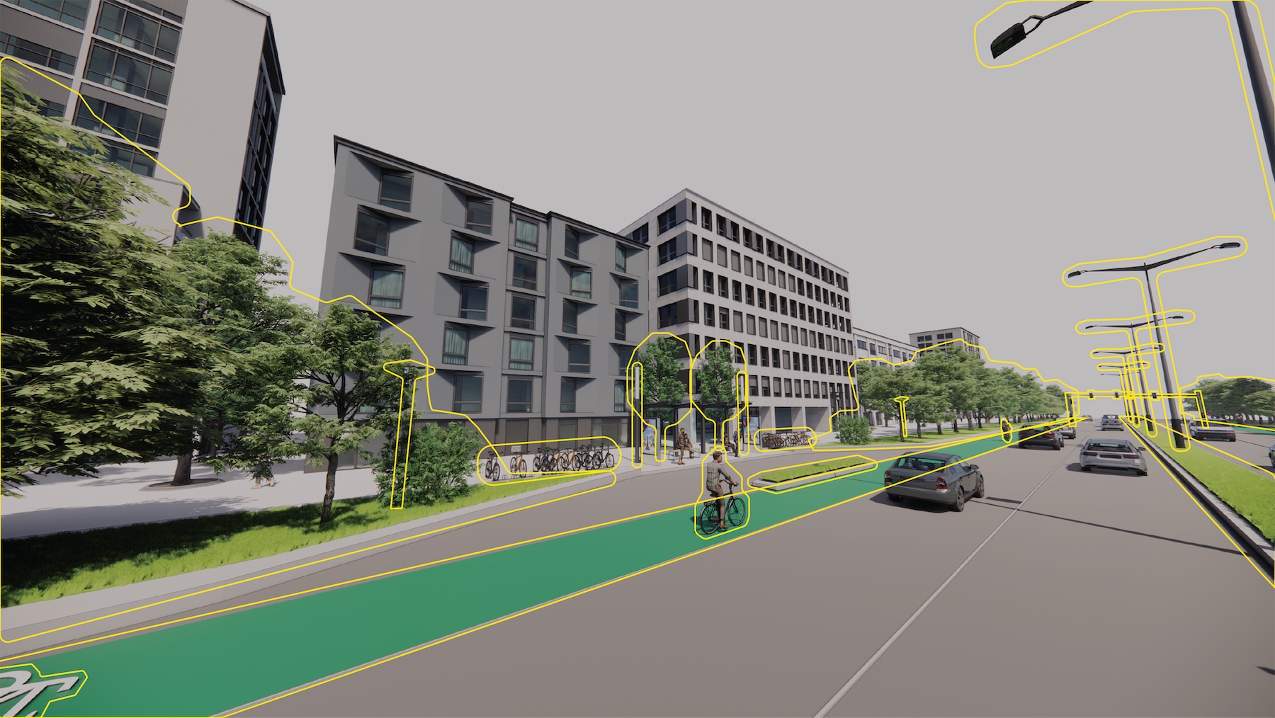
Figure 1: Illustration of an urban setting together with one of the corresponding street-level views, highlighting several aspects that may indicate bikeability. The method presented in this paper takes advantage of a substantial number of visual features that may be extracted automatically from street view images and engage them to generate a composite index that suggests cycling appeal at a fine spatial scale and across multiple cities.

Considering the developments in computer vision and proliferation of street view imagery (e.g. increased coverage of commercial services such as Google Street View and introduction of crowdsourced alternatives), we believe that such research is needed and timely. This study tests a hypothesis that CV and SVI coupled together have a strong potential to overcome the issues faced by conventional methods in gauging how friendly urban streets are to cyclists. Further, as the availability of SVI is now considered to be virtually omnipresent, a notable research gap is comparative studies that involve more than one city. Thus, in this study we aim to answer the following research questions: can we use CV techniques and SVI data to comprehensively assess bikeability within and among cities? If yes, can SVI and CV alone be used to assess bikeability, replacing traditional techniques entirely? To answer these questions, we develop a bikeability index with 34 indicators under five categories and implement it in Singapore and Tokyo. The contributions of our study are the novel investigation of CV techniques’ and SVI indicators’ usefulness in comprehensive bikeability assessment, construction of a new comprehensive bikeability index regarding an unprecedented amount of aspects, and provision of a new data collection method that can extract subjective and objective indicators from street-level information at a larger spatial scale and across multiple geographies, thereby overcoming the issues found by the previous studies. We believe that the method and the index may be scaled around the world, including additional cities in future work. It is important to note that our method includes also a survey with a large number of human participants to investigate whether CV techniques may estimate human perception of cycling appeal automatically.

In Section 2, we conduct a comprehensive literature review to affirm the research gap. The comprehensive and structured overview of the state of the art is another contribution of this paper. Section 3 explains the data sources and methodologies used in this study. Section 4 describes the results of this study together with a discussion. Finally, we conclude our study as well as discuss further directions for future research in Section 6.

2 Related work

2.1 Bikeability studies

Many studies have explored various aspects of the built environment that can influence people’s cycling behavior (Bauman et al., 2012; Nielsen and Skov-Petersen, 2018; Pritchard et al., 2019; Daraei et al., 2021; Kraus and Koch, 2021; Nazemi et al., 2021; McNeil, 2011; Ma and Dill, 2017; Cicchino et al., 2020; Nogal and Jiménez, 2020; Sottile et al., 2019; Berger and Dörrzapf, 2018; Porter et al., 2018; Aldred et al., 2020; Long and Zhao, 2020; Doubleday et al., 2021; Brüchert et al., 2020; Martin et al., 2021; Attard et al., 2021). Studies on the association of the built environment and cycling conditions became well-established, and many researchers developed indexes to assess specific aspects of the built environment that can affect cycling behavior and comprehensively quantify bikeability, i.e. the extent to which an environment is friendly for bicycling.

In the early days of related work between 2010 and 2015, methodologies to collect data are mostly conducted through field surveys, thus tending to be time- and resource-intensive. Studies by Hoedl et al. (2010), Horacek et al. (2012), and Koh and Wong (2013) involve field observation by experts, and such a methodological limitations precludes bikeability assessment at large scales. Moreover, only a few studies (Koh and Wong, 2013) include both objective and subjective indicators, and most of the studies (Wahlgren et al., 2010; Hoedl et al., 2010; Horacek et al., 2012) only focused on either one of the indicators. The spatial granularity of sample points is loosely defined and not standardized in some studies as well (Wahlgren et al., 2010; Horacek et al., 2012).

Recent bikeability studies have become more standardized and scalable. Although some studies still use field observation (Manton et al., 2016; Cain et al., 2018), more studies apply emerging technologies and data sources such as remote sensing images, manual virtual auditing using SVI, and crowdsourcing, to collect data (Krenn et al., 2015; Gullón et al., 2015; Winters et al., 2016; Kalvelage et al., 2018), enabling large-scale and comparative assessment of bikeability. However, as data collection methods become more scalable, subjective indicators are excluded by many studies (Krenn et al., 2015; Manton et al., 2016; Winters et al., 2016; Cain et al., 2018; Kalvelage et al., 2018). Moreover, remotely sensed imagery cannot capture street-level information, and manual virtual auditing and crowdsourcing data collection require a large amount of time and resources. For example, a recent study by Arellana et al. (2020) utilizes virtual auditing in SVI, but this data collection process was reported to be six months long for a city-scale study area, suffering from the same issue of a time-intensive method as the aforementioned studies. To overcome the issue of the balance between street-level information and scalability, recent studies couple SVI with CV techniques to automate the indicator extraction (Gu et al., 2018; Tran et al., 2020), but the number of indicators extracted by such methods remains still limited. Moreover, subjective indicators for bikeability assessment have not been extracted from SVI by using CV yet. Therefore, there is a need for further studies to examine the possibility of extracting more indicators — both objective and subjective — from SVI by using CV.

Structuring the rundown on related work, Table 1 summarizes indicators used in the reviewed studies. Most of the indicators could be categorized into connectivity, environment, infrastructure, vehicle–cyclist interaction (V–C interaction), and perception. In developing bikeability indexes, the previous studies have faced the issues of the time-intensive data collection process, the balance between subjectivity and objectivity, extraction of street-level information, and standardization of spatial granularity. Table 2 summarizes the issues mentioned above. Literature reviews on bikeability by Kellstedt et al. (2021) and Castañon and Ribeiro (2021) indicate that the past development of bikeability assessment has been driven by innovative uses of advanced new technologies, thereby suggesting that newer technologies may overcome these issues mentioned above. While there have been studies that have utilized SVI and CV techniques to assess bikeability, and thus indicating the reliability of SVI as a data source that can be used in a scalable manner, they suffer from shortcomings that we seek to mitigate in our work. Primarily, previous studies used these technologies to assess very limited aspects of bikeability (i.e. only up to a few indicators), did not collect and assess subjective indicators, and have been evaluated on limited areas. Such a gap necessitates further studies to examine how much SVI and CV techniques are usable to assess bikeability comprehensively.

2.2 Street view imagery in urban studies

The growth of the spatial coverage of street view imagery and the development of computer vision techniques have catalyzed the recent proliferation of studies that utilize them, both in transportation and urban planning and beyond (Wang et al., 2019b; Song et al., 2020; Wu and Biljecki, 2021; Ye et al., 2020; Fan et al., 2021; Chen et al., 2021a). This section focuses on studies that use SVI to extract information of data used in previous bikeability studies under four categories that have been delineated by this study (i.e. environment, infrastructure, vehicle-cyclist interaction, and perception), and to examine subjects pertaining to cycling.

One of the more explored aspects in related research is urban greenery. Quantification of greenery by using image segmentation, CV techniques that can classify categories of objects at a pixel-level, has enabled many various urban studies ranging from simple assessment of the distribution of vegetation and interdisciplinary examinations of the relationships between greenery and various aspects of cities, such as physical activities of residents and real estate (Ye et al., 2019a; Lu, 2019; Ye et al., 2019b). Other studies quantify greenery, sky view factor (i.e. openness), and buildings (i.e. enclosure) with semantic segmentation to measure characteristics of cities in a scalable manner (Li et al., 2017; Gong et al., 2018, 2019; Li and Ratti, 2019; Toikka et al., 2020; Wang and Vermeulen, 2020; Ma et al., 2021; Zhou et al., 2021). These features that are extracted from SVI, which have been leveraged for a variety of applications, can be also used to evaluate bikeability.

The high scalability of CV techniques and SVI has also multiplied opportunities for infrastructure assessment at a city scale. Hall et al. (2018) propose a methodology to detect and classify traffic signals, and Chacra and Zelek (2018) develop a CV-based model to detect infrastructure anomalies from SVI. Assessment of urban accessibility is conducted by Najafizadeh and Froehlich (2018), developing models to detect accessibility problems from SVI, such as missing curb ramps and street surface issues. Further, Ding et al. (2021) use object detection and classification CV models to map bike lane networks from SVI. Mapillary, a crowdsourced SVI service, developed a dataset called Vistas, which contains 25,000 images collected from around the world, and annotated according to 66 categories (Neuhold et al., 2017). Cityscapes is another frequently used street-level dataset for segmentation (Cordts et al., 2016; Gong et al., 2019; Nagata et al., 2020). Although Mapillary Vistas has many infrastructure-related categories (e.g. bike lane and bike parking) that other segmentation training datasets do not regard, it has not been widely used in urban studies. Thus, using this dataset might expand the prospects of SVI for bikeability assessment.

These techniques have been utilized in transport studies as well. Goel et al. (2018) find that the number of cyclists manually counted in GSV images is strongly correlated with the cycling mode share reported by cities in the UK (r = 0.92). Zhang et al. (2019a) and Chen et al. (2020a) also examine the relationship between visual features and urban traffic volume and reveal that SVI can be used to explain more than 65 percent of the spatiotemporal mobility pattern. These findings hint that SVI may be used to estimate traffic volume, which is an important aspect of bikeability (Labetski and Chum, 2020).

Table 1: An overview of indicators used by previous studies grouped into five categories.

Publication	Connectivity	Environment	Infrastructure	V-C interaction	Perception
Clifton et al. (2007)	Cul-de-sac	Land use	Sidewalk		Attractiveness
	Continuity	Slope	Pavement	Traffic speed	Safety
		Greenery	Path obstruction	Street parking	Cleanliness
		Enclosure	Sidewalk buffer	Traffic control
		Building design	Road condition
		Setback	Curb cuts
			Crossing
			Street light
			Street amenity
			Directional sign
			Power line
			Bike lane
			Transit facilities
Hoedl et al. (2010)	N/A	Greenery	Bikelane		N/A
		Land use	Sidewalk	Traffic speed
		Billboards		Traffic volume
		Open space
Wahlgren et al. (2010)	Directness	Air quality	N/A	Traffic speed	Attractiveness
	Intersection	Noise		Traffic volume	Crowdedness
		Greenery		Cylist speed	Safety
		Slope		Traffic separation	Beauty
Horacek et al. (2012)	N/A	Slope	Pavement	Traffic speed	Beauty
			Street light	Traffic volume
			Potholes	Traffic control
			Path size
			Sidewalk buffer
			Curb cut
			Bike lane
Koh and Wong (2013)	Detour	Slope	Directional sign	N/A	Safety
	Intersection	POIs	Pavement		Crowdedness
		Greenery	Shelter
		Water
Gullón et al. (2015)	Different routes	Greenery	Pavement		Cleanliness
		Land use mix	Street amenity	Traffic control	Beauty
			Street light		Attractiveness
			Crossing
Krenn et al. (2015)	N/A	Greenery	Bike lane	Traffic separation	N/A
		Water
		Slope
Manton et al. (2016)	Intersection	N/A	Road width	Traffic volume	N/A
				Street parking
				Traffic separation
Winters et al. (2016)	Intersection	Slope	Bike lanes	Mode share	N/A
	Distance to POIs
Hartanto et al. (2017)	Intersection	Water	Road type	Traffic speed	N/A
	Directness	Greenery	Pavement	Traffic volume
		Buildings	Street light
		Slope	Bike parking
Cain et al. (2018)	Intersection	Land use	Transit facilities	Traffic control	N/A
	Informal path	No. of pedestrian	Roll-over curb
	Cul-de-sac	Water	Street amenity
		Landscape	Bike parking
		Hardscape	Curb cuts
		Graffiti	Bike lane
		Setback	Crossing
		Shade	Road width
		Building design	Sidewalk buffer
			Bike lane
			Sidewalk
Gu et al. (2018)	Street density	Shade	Bike lane	Traffic separation	N/A
		POIs	Crossing
Arellana et al. (2020)	N/A	Slope	Bike lane	Traffic control	N/A
		Greenery	Sidewalk	Mode share
		Building design	Street obstruction	Traffic speed
		Crime presence	Bike lane width
			Street light
			Police presence
			Security camera
Tran et al. (2020)	Directness	POIs	Bike lane	N/A	N/A
		Greenery
		Enclosure
		Crowdedness

Table 2: Characteristics of methods used by previous studies.

Publication	Data	Weighting system	No. of indicators by SVI+CV	Street-level information
Clifton et al. (2007)	Objective &	Individual assessment	0	Yes
	Subjective
Hoedl et al. (2010)	Objective	Individual assessment	0	Yes
Wahlgren et al. (2010)	Subjective	Individual assessment	0	Yes
Horacek et al. (2012)	Objective	Unequal arbitrary weight	0	Yes
Koh and Wong (2013)	Objective &	Survey-based weight	0	Yes
	Subjective
Gullón et al. (2015)	Objective &	Unequal arbitrary weight	0	Yes
	Subjective
Krenn et al. (2015)	Objective	Equal weight	0	No
Manton et al. (2016)	Objective	Regression modeling	0	Yes
Winters et al. (2016)	Objective	Equal weight	0	No
Hartanto et al. (2017)	Objective	Equal weight	0	Yes
Cain et al. (2018)	Objective	Unequal arbitrary weight	0	Yes
Gu et al. (2018)	Objective	Entropy weight	3	No
Arellana et al. (2020)	Objective	Survey-based weight	0	Yes
Tran et al. (2020)	Objective	Equal weight	3	Yes

Extraction of information from images has also enabled the prediction of urban perception based on SVI. Naik et al. (2014) conduct surveys on safety, in which 7,872 unique participants from 91 countries ranked 4,109 images using 208,738 pairwise comparisons. Dubey et al. (2016) develop a dataset called Place Pulse 2.0, which consist of 110,988 images from 56 cities and 1,170,000 pairwise comparisons answered by 81,630 online survey participants on six perception scores, and predicted these scores with convolutional neural network models, such as VGGNet, and this study’s dataset and methodology have been utilized and replicated by other studies (Kang et al., 2021; Qiu et al., 2021). Yao et al. (2021) conduct a similar study to predict perception scores by surveying 20 volunteers on 1,000-2,000 images and predicting perception scores using a random forest model and features extracted by FCN-8s as inputs. Verma et al. (2020) also recruit only 79 participants to rate 200 images, extracting high- and low-level features from SVI by using CV techniques (e.g. image segmentation, object detection, classification, and edge detection), and designing models to predict fourteen perception scores, such as “pleasant”, “boring”, and “safe”. Moreover, the validity of conducting perception surveys has been examined and found to be as reliable as surveys based on the real environment by Feng et al. (2021).

Lu et al. (2019) and Wang et al. (2020) examine the association between urban greenery (extracted from SVI) and cycling behaviors, and Hollander et al. (2020) study the correlation between transportation planning and the perceived safety of the built environment. A study by Tran et al. (2020) is the only study that relies on SVI to create a bikeability index, but this study uses SVI only to assess very limited aspects of bikeability, such as greenery and enclosure. Therefore, there has not been any study that developed a comprehensive bikeability index mirroring the wide array of aspects jointly covered by related work and one that has utilized SVI as a major data source to calculate it, a gap that is bridged by our study.

2.3 Summary

The literature review elucidates the proliferation of urban studies that utilize SVI and CV techniques and, at the same time, it exposes the absence of studies that take advantage of them for assessing cycling appeal and developing a bikeability index. Such omission is possibly caused by obstacles of using CV techniques and the complexities of developing a comprehensive bikeability index system. However, previous studies demonstrate the possibility of replacing traditional data collection for bikeability indicators, as they collect information on similar aspects that may indicate cycling appeal.

This paper aims to bridge this gap by designing a thorough bikeability index that is largely derived using SVI and CV, and it also uses the opportunity to critically investigate their value and independence when doing so. Moreover, as SVI data has virtually global coverage, the study puts scalability under the spotlight; thus, the combination of scalability of SVI and efficient extraction of indicators through CV can reduce the time and resource cost of bikeability assessment compared to conventional data sources and methods. Finally, potential barriers of this approach for urban planners are also examined to understand its application and prospects for adoption.

3 Methodology

This study uses six data sources (i.e. SVI, surveys, OpenStreetMap (OSM), Land Use (LU), Digital Elevation Model (DEM), and Air Quality Index (AQI)) to evaluate 34 indicators under five categories (i.e. connectivity, environment, infrastructure, perception, and vehicle-cyclist interaction). The comprehensive selection of these indicators is a contribution on its own, as its scope is unprecedented, and may serve as a resource to develop indexes in other domains. Testing the scalability of the method, Singapore and Tokyo, as two geographies with disparate characteristics, are selected as study areas. Thus, data retrieval and indicator extractions are conducted to develop the composite index by weighting each category and indicator equally. Figure 1 highlights some examples of phenomena in SVI that are characterized in this method.

3.1 Selection of indicators

Conducting a review of studies that developed bikeability indexes, this study devised an exhaustive list of indicators used by them (Hartanto et al., 2017; Winters et al., 2016; Gullón et al., 2015; Wahlgren et al., 2010; Horacek et al., 2012; Hoedl et al., 2010; Clifton et al., 2007; Manton et al., 2016; Cain et al., 2018; Koh and Wong, 2013). This inventory was used to create an own index to expand related work and minimize the bias when selecting indicators. Duplicates and those indicators that cannot be obtained and/or are unsuitable for this study have been excluded, such as noise and the presence of informal paths and crimes. After filtering, out of 65 unique indicators found in the previous studies in total, 34 indicators (i.e. about 52%) were kept, forming the most extensive instance to date. Future studies can use our method while partially modifying this list to incorporate more or fewer indicators as long as they can be extracted from the data sources we used.

These 34 unique indicators are categorized into five categories, namely, connectivity, environment, infrastructure, perception, and vehicle-cyclist interaction (see Table 3). Regarding data sources, 21 indicators are to be extracted from SVI, 10 from OSM, one from each of LU, DEM, and AQI.

Although this study does not examine if the selected indicators can predict bike usage, most of the reviewed previous studies also selected them based on literature reviews, except for a few (Winters et al., 2016; Arellana et al., 2020) that use regression analysis. Moreover, higher bikeability does not necessarily lead to higher counts of bike usage. For example, Arellana et al. (2020) examine and find that other factors, such as population density and socio-economic characteristics, also play a role (Munira et al., 2021). Therefore, investigating whether the bikeability index can predict bike usage is out of the scope of this research.

Table 3 lists indicators with their data sources, extraction methods, and scaling methods. For scaling methods, min-max scaling and negative min-max scaling were used (see Equation 1 and Equation 2). The sampling method is further explained in the following sections.

$$x_{\text{Min-Max Scaled}}=\frac{x-\min(x)}{\max(x)-\min(x)}$$ (1)

$$x_{\text{Negative Min-Max Scaled}}=1-\frac{x-\min(x)}{\max(x)-\min(x)}$$ (2)

3.2 OSM and SVI data retrieval

This study relies on OSM to retrieve information on indicators and also for the retrieval of locations on streets that are used to fetch street view images. The completeness of OSM in the study area is deemed adequate (Barrington-Leigh and Millard-Ball, 2017; Biljecki, 2020). To retrieve the OSM data, OSMnx (Boeing, 2017) was used, obtaining about 250,000 points and 440,000 points for Singapore and Tokyo, respectively. After that, 7,142 points were randomly selected. The number of points to be collected was set at 7,142 because this is the maximum number of SVI images that can be retrieved within the free credit provided by GSV API every month. Future studies can also utilize the initial trial credit as well, but if there are financial constraints, the rise of volunteered SVI, such as KartaView and Mapillary, may ameliorate this issue in the future. For this study, the API of GSV was used to collect images because of its extensive coverage and high quality in both metropolises.

Table 3: Indicators forming the comprehensive bikeability index introduced by this study.

Indicators	Data	Extraction	Scale
Connectivity
No. of intersection with lights	OSM	Aggregation (500m)	0-1 (Negative Min-Max)
No. of intersection without lights	OSM	Aggregation (500m)	0-1 (Negative Min-Max)
No. of cul-de-sac	OSM	Aggregation (500m)	0-1 (Negative Min-Max)
Environment
Slope	DEM	Calculation	0-1 (Negative Min-Max)
No. of POI	OSM	Aggregation (500m)	0-1 (Min-Max)
Shannon land use mix index	Land use	Aggregation (500m)	0-1 (Min-Max)
Air quality index	AQI	Spatial interpolation	0-1 (Negative Min-Max)
Scenery: greenery	SVI	Segmentation	0-1 (Min-Max)
Scenery: buildings	SVI	Segmentation	0-1 (Min-Max)
Scenery: water	SVI	Segmentation	0-1 (Min-Max)
Infrastructure
Type of road	OSM	Aggregation (100m)	service, track = 0.1
			primary, primary_link = 0.2
			secondary, secondary_link = 0.4
			tertiary, tertiary_link = 0.5
			unclassified = 0.6
			pedestrian path = 0.8
			cycleway = 1
			Others = 0
Presence of potholes	SVI	Segmentation	1 if not present
			0 if present
Presence of street light	SVI	Segmentation	1 if present
			0 if not present
Presence of bike lanes	SVI	Segmentation	1 if present
			0 if not present
No. of transit facilities	OSM	Aggregation (500m)	0-1 (Min-Max Scale)
Type of pavement	OSM	Aggregation (100m)	unhewn_cobblestone, cobblestone = 0.2
			sett, metal, wood = 0.4
			paved = 0.5
			concrete:lanes, plates, paving_stones = 0.6
			asphalt, concrete = 1
			Others = 0
Presence of street amenities	SVI	Segmentation	1 if present
			0 if not present
Presence of utility pole	SVI	Segmentation	1 if not present
			0 if present
Presence of bike parking	SVI	Segmentation	1 if present
			0 if not present
Road width	OSM	Aggregation (100m)	0-1 (Divide by 10)
			1 if width is larger than 10m
Presence of sidewalk	SVI	Segmentation	1 if present
			0 if not present
Presense of crosswalk	SVI	Segmentation	1 if present
			0 if not present
Presence of curb cuts	SVI	Segmentation	1 if present
			0 if not present
Perception
Attractiveness for cycling	SVI	Surveys, Modeling	0-1 (Min-Max)
Spaciousness	SVI	Surveys, Modeling	0-1 (Min-Max)
Cleanliness	SVI	Surveys, Modeling	0-1 (Min-Max)
Building design attractiveness	SVI	Surveys, Modeling	0-1 (Min-Max)
Safety as a cyclist	SVI	Surveys, Modeling	0-1 (Min-Max)
Beauty	SVI	Surveys, Modeling	0-1 (Min-Max)
Attractiveness for living	SVI	Surveys, Modeling	0-1 (Min-Max)
Vehicle-Cyclist Interaction
No. of vehicles	SVI	Detection, Aggregation (500m)	0-1 (Negative Min-Max)
Presence of on-street parking	OSM	Aggregation (100m)	1 if not present
			0 if present
Presence of traffic lights / stop signs	SVI	Segmentation	1 if present
			0 if not present
No. of speed control devices	OSM	Aggregation (100m)	1 if present
			0 if not present

3.3 Extraction of indicators

The feature extraction process for indicators differs among different categories and data sources. Feature extractions for land use, topography, and AQI are relatively straightforward. For land use, we use an entropy formula derived from the Shannon index developed by Frank et al. (2005) within 500m buffers from sample points (see Equation 3).

$$LUM=-1\left(\sum_{i=1}^{n}p_{i}*\ln(p_{i})\right)/\ln(n)$$ (3)

In this formula, $LUM$ is the land-use mix score, $pi$ is the proportion of the neighborhood covered by the land use $i$ against the total area for all the land-use categories, and $n$ is the number of land-use categories. A land-use mix score of 1 indicates the highest mix possible while a score of 0 indicates the area contains a single land use. This results in values between 0, the lowest mixed-use level, and 1, the highest mixed-use level.

For topography, the slope is calculated from DEM data created by Yamazaki et al. (2017) and sampled at each sample point, and the value was scaled with min-max scaling.

AQI data is collected from the Air Quality Index by automating the retrieval of stations and AQI data in both cities with a Python library called Selenium. The annual average AQI of stations in the cities is calculated by taking the daily maximum value of various pollutants (e.g. PM2.5) in the unit of µg/m3, and then spatial interpolation was conducted to estimate the average AQI at the sample points in this study by using inverse distance weighted interpolation (see Equation 4).

$$z_{p}=\frac{\sum_{i=1}^{n}\left(\frac{z_{i}}{d_{i}^{p}}\right)}{\sum_{i=1}^{n}\left(\frac{1}{d_{i}^{p}}\right)}$$ (4)

In this formula, $z_{p}$ denotes the interpolated values of the target points, $n$ represents the number of points used to interpolate from, $z_{i}$ shows the value being interpolated from, and $d_{i}^{p}$ is the distance between the target point and the point being used to interpolate from. The calculated AQI is then scaled into values between 0 and 1 by using min-max scaling.

Feature extractions from OSM are conducted by taking buffers from sample points. For the density of intersection with/without lights, cul-de-sac, shops along the route, and transit facilities, we created 500m buffers from sample points and aggregated the number of these indicators because we need to consider the surrounding contexts as well. Other indicators collected from OSM, such as the type of roads and the type of pavement, are collected by creating 100m buffers from sample points and converting categorical values to numerical if necessary.

Finally, this study conducts feature extractions from SVI in two ways. For objective indicators, two CV techniques — segmentation and object detection — were used to extract features. For segmentation, the In-Place Activated BatchNorm model trained on Mapillary Vistas with WideResNet38 and DeepLab3 developed by Bulò et al. (2018) is selected because of its high accuracy of the mean intersection over union of 53.42%. Indicators such as the scenery along bike lanes (i.e. built-up area, greenery, sky view factor, water) are quantified by calculating the ratios of the pixels categorized as them over the total number of pixels in the image, which are then scaled into between 0 and 1 with min-max scaling. Because it is not meaningful to calculate pixels of other objects such as street lights, bike lanes, street amenities, and bike parking, they are quantified in a binary manner (i.e. score 1 if they are in the image and 0 if they are not in the image). Object detection is used for one indicator, that is, the number of vehicles, as a previous study suggests that SVI can be used to estimate the traffic in the area (Zhang et al., 2019a). For this task, we opt for the GluonCV’s model zoo developed by Guo et al. (2020) and select a YOLOv3 model pre-trained on Pascal VOC dataset with Darknet53 as the base model, which can detect the number of bicycles, pedestrians, and vehicles with an average precision of 58.2% at the intersection over a union of 0.5. We chose this model because of its reported relatively high speed and accuracy compared to other models, such as Faster Region-based Convolutional Neural Networks and Single Shot Detection (Srivastava et al., 2021; Li et al., 2020). Moreover, the core of our paper is separate from the models, thus if necessary, new models can be used in any part of this methodology, as our approach is model-agnostic. Because a street view image captures only the traffic volume of the road segment at that moment, it is not entirely reliable to estimate the traffic based on just one photo at a point. Therefore, a buffer of 500m was generated for each point, aggregating the number of vehicles found in the plentiful imagery in the buffer. After this processing, the mode share was also scaled into values between 0 and 1 by min-max scaling. A previous study (Chen et al., 2020a) uses a similar method to estimate the number of pedestrians and obtains Cronbach’s alpha above 0.8, indicating SVI’s high reliability as a data source. However, it should be noted that the number of images within each buffer varies because the sample points were randomly selected, which might produce some bias. Also, duplication of vehicles detected in SVI can cause bias because some vehicles could have driven together with the vehicles collecting the street view images. The aforementioned study (Chen et al., 2020a) did not consider this issue and still obtained high reliability; thus, we leave improvement in methodology to detect the same vehicles with models such as Siamese-convolutional neural network for future studies.

Subjective indicators are under the perception category, including attractiveness for cycling, spaciousness, cleanliness, building design attractiveness, and perception of safety as a cyclist, and these indicators were predicted by using features extracted from SVI. We follow the methodology used by Verma et al. (2020), where high- and low-level features of images are used to predict perceptions of images (see Table 4). Low-level features can be extracted through edge detection, blob detection, and Hue-Saturation-Lightness (HSL) extraction. Edges are quantified by detecting edges and calculating the ratio of pixels that are categorized as edges over the total number of pixels. Blob detection was used to calculate the number of blobs in SVI, and HSL extraction is conducted to calculate the average and standard deviation of each hue, saturation, and lightness. It should be noted that lightness might have some bias because of variances in the time when the images were collected, although GSV has a standardized data collection procedure and post-processing of images (Google, 2018). As for high-level features, image classification (IC), object detection (OD), and semantic segmentation (SS) are used to extract them. For OD and SS, this study uses the same models mentioned above, and a ResNet50 model trained on Places365 data with an accuracy of 85.07% is used for IC (Zhou et al., 2018). These extracted features are dependent variables to predict the perception indicators.

Table 4: Features for predicting perception.

Visual features	Definitions
tree_ss	% of pixels classified as trees.
sky_ss	% of pixels classified as the sky.
street_ss	% of pixels classified as street and sidewalks.
built_ss	% of pixels classified as buildings.
others_ss	% of pixels classified as other remaining outdoor classes.
nature	% of pixels classified as natural elements such as sky, tree, and water.
shannon	Shannon entropy values calculated on SS task.
slum_ic	Probability of being classified as Slum/Alley/Junkyard in IC task.
market_ic	Probability of being classified as Bazaar/Flea market/Market in IC task.
built_other_ic	Probability of being classified as Downtown/Embassy/Plaza in IC task.
green_other_ic	Probability of being classified as Forest path/Forest road in IC task.
bicycle_od	No. of bicycles detected in OD task.
bus_od	No. of buses detected in OD task.
car_od	No. of cars detected in OD task.
motorcycle_od	No. of motorcycles/scooters detected in OD task.
person_od	No. of persons detected in OD task.
traffic_light_od	No. of traffic lights detected in OD task.
truck_od	No. of trucks/auto rickshaws detected in OD task.
canny_edge_llf	% of pixels detected as edges.
no_of_blobs_llf	No. of blobs.
hue_mean_llf	The mean value of the hue dimension in HSL color space.
hue_std_llf	The standard deviation of the hue dimension in HSL color space.
lightness_mean_llf	The mean value of the lightness dimension in HSL color space.
lightness_std_llf	The standard deviation of the lightness dimension in HSL color space.
saturation_mean_llf	The mean value of the saturation dimension in HSL color space.
saturation_std_llf	The standard deviation of the saturation dimension in HSL color space.

To collect the training data set and build models to predict indicators suggesting perception, a survey is conducted on Amazon Mechanical Turk, for which this study has received an exemption from the Institutional Review Board of the National University of Singapore, and in which the participants were compensated financially. For each city, 400 SVIs, i.e. 800 in total, were randomly selected for the survey, which was designed to have at least eight different participants rate the images on the five indicators on a scale of 0 to 10. The large number of participants to rate each image ensures reliability. The occasional and inevitable outliers among the responses were detected with the median absolute deviation method and removed when the output is above three (see Equation 5).

$$\operatorname{MAD}=\operatorname{median}\left(\left|X_{i}-\tilde{X}\right|\right)$$ (5)

$X_{i}$ denotes each observation, and X̃ represents the median of all the observations.

The collected dataset is split into training and validation data sets in an 80:20 ratio to build predictive models with LightGBM (Ke et al., 2017), which is gaining momentum in urban studies (Chen et al., 2021b) for its high accuracy and low computational cost in training (Zhang et al., 2019b; Deng et al., 2018). In this study, we tuned the following hyperparameters with 10-fold cross-validation: num_leaves, max_depth, min_child_samples, min_child_weight, subsample, colsample_bytree. After conducting the prediction for the rest of the points, the predicted perception indicators are scaled into values between 0 and 1 with min-max scaling.

Moreover, this study explores the relationships between all the features and perception scores by grouping observations into below- and above-average values of features and conducting Welch’s t-test (Delacre et al., 2017). We aim to reveal the underlying visual effects of each feature on human perceptions.

3.4 Development of a new composite index to assess bikeability

The composite index of this study, one of its advancements and key contributions, is developed based on conflating bikeability indexes developed by previous studies. There are three types of weighting systems developed by them, which warrant a brief overview. One of them is the independent assessment of indicators. This method only evaluates each indicator but does not give weights to them, and it is used by Wahlgren et al. (2010) and Hoedl et al. (2010). Another type is the arbitrary weight. This method gives arbitrary weights to categories and indicators, which is adopted by Cain et al. (2018); Horacek et al. (2012). The last type is equal weight. This method gives equal consideration to all the categories and indicators, which actually — strictly speaking — belongs to the arbitrary weighting system, but this study differentiated them for clarity. This method is used by Hartanto et al. (2017), Winters et al. (2016), and Tran et al. (2020), and it is a common system among the reviewed studies. This study adopts the equal weight system for its simplicity and scaled all the indicators into values between 0 and 1 to prevent any indicators from excessively influencing the composite index at the end (see Equation 6).

$$Index=\sum_{i=1}^{n}\left(x_{i}*(100/(N_{c}*N_{ci}))\right)$$ (6)

In this equation, Index represents the bikeability index, $x_{i}$ denotes the value of each indicator $i$, $N_{c}$ show the number of categories, and $N_{ci}$ stand for the number of indicators in the respective category.

Facilitating a critical analysis of the value of SVI over non-SVI counterparts, as one of the principal aims of this study, the following indexes with different types of indicators are designed:

1. Index with SVI indicators and non-SVI indicators

2. Index with only SVI indicators

3. Index with only non-SVI indicators

These indexes and their sub-categories were compared with each other to examine how much SVI and non-SVI indicators explain the overall variance. Finally, Figure 2 sums up the methodology.

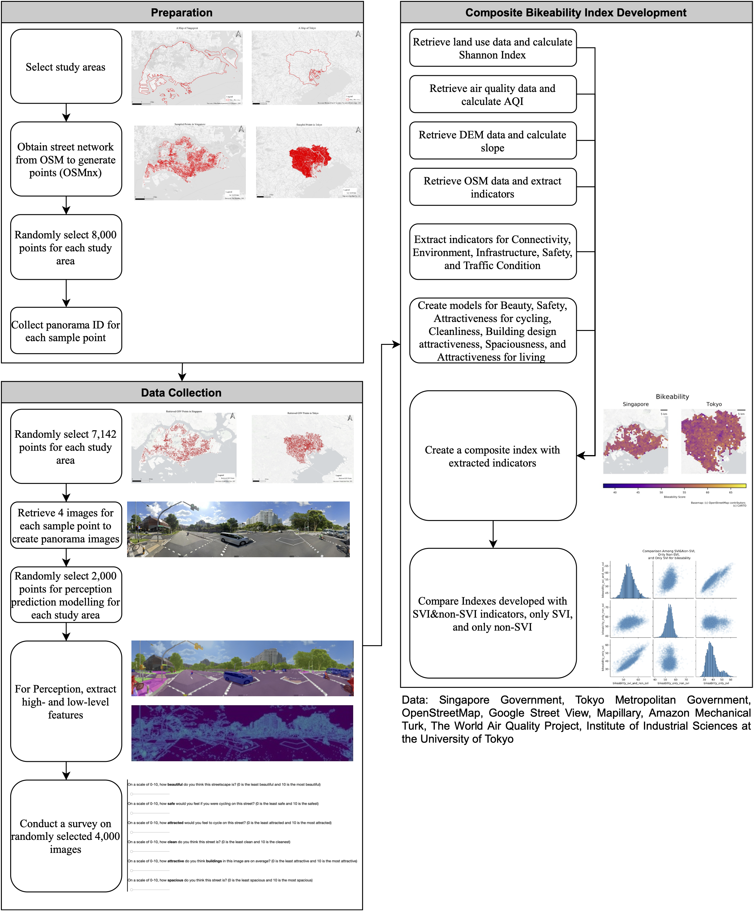
Figure 2: Illustration of the methodology of this study.

4 Results

4.1 Data collection

For OSM data, street network data and point data were retrieved. For street network data, 252,369 street segments and 450,379 street segments were retrieved for Singapore and Tokyo, respectively. As for point data, 12,640 POIs and 157 mass rail transit stations were collected from Singapore, 75,203 POIs, and 606 stations were collected from Tokyo. For SVI, after removing indoor images and grey images from 7,142 images, 5,833 and 6,181 panorama images remained for the two cities.

For LU, each city’s open data by the local government was used (Tokyo Metropolitan Government, 2018; Singapore Government, 2020b). Because the categorizations of LU in each city were different, LU categories were harmonized to residential, commercial, and industrial in this study, and other categories were excluded. AQI data in 2020 are obtained for 5 and 126 stations in the city-state and the Japanese capital, respectively.

4.2 Extracted indicators and composite index

4.2.1 Connectivity

Connectivity is assessed based on the number of intersections with lights, intersections without lights, and cul-de-sacs. Comparing Singapore and Tokyo, the latter achieves higher scores for connectivity (see Table 6 and Figure 8). Due to a large number of indicators not all of them can be detailed in this paper, but as an example, Figure 3 illustrates the distribution of values in this particular indicator. The score for the number of intersections without traffic lights is much lower for Singapore while the other two indicators have a similar distribution.

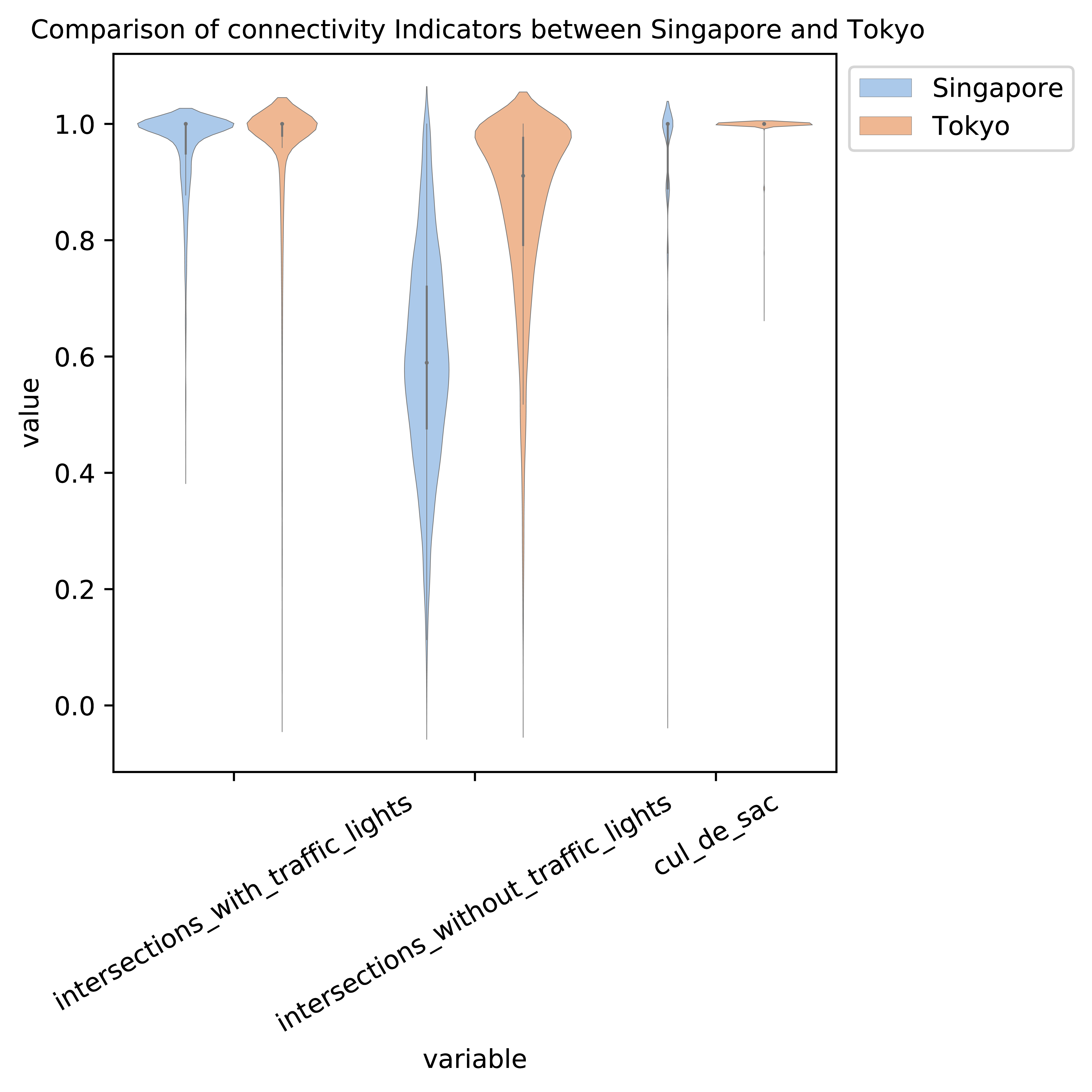
Figure 3: Distribution of indicators describing connectivity across numerous locations in Singapore and Tokyo.

4.2.2 Environment

The environment is evaluated based on slope, the number of POIs, land use mix, AQI, and pixel ratios of greenery, buildings, and water, aiming to evaluate the natural and built environment. Compared to Singapore, Tokyo has a higher mean score for this category (see Table 6 and Figure 8). The distributions of each indicator suggest that Tokyo obtains noticeably higher scores for slope, land use, the pixel ratio of buildings. Such results reflect Tokyo’s relatively flat topography, organic distribution of land uses, and densely built buildings that create more enclosures for cyclists. Singapore achieved higher scores in AQI and greenery, which also reflects its strategic environmental management as a garden city (Han, 2017; Palliwal et al., 2021).

4.2.3 Infrastructure

Infrastructure is evaluated based on the type of road and pavement, the width of the road, number of transit facilities, and presence of potholes, street lights, bike lanes, street amenities, utility poles, bike parking spaces, sidewalks, crosswalks, and curb cuts. This category aims to comprehensively evaluate various elements in the realm of infrastructure. Compared to Tokyo, Singapore achieves a much higher mean score for this category (see Table 6 and Figure 8). Singapore obtains higher scores in the type of pavement (i.e. surface), the presence of street amenity, and, especially, utility poles, which show the nearly opposite result from Tokyo. This result reflects Tokyo’s issue with many utility poles, which not only deteriorates the beauty of the city but also can cause obstruction for pedestrians and cyclists (Inajima and Urabe, 2017).

4.2.4 Vehicle-cyclist interaction

Vehicle-cyclist interaction was evaluated based on the number of vehicles and speed control devices and the presence of on-street parking and traffic lights/stop signs. This category aims to assess how safely cyclists interact with vehicles; thus, fewer and slower traffic leads to higher scores. The mean scores for both cities are also similar, while Singapore has a slightly higher mean and standard deviation (see Table 6 and Figure 8). The analysis suggests very small variances in the indicators and similar distributions for both cities. Such a result can potentially be explained: Singapore and Tokyo have similar restrictions on vehicles; for example, on-street parking is strongly discouraged in both cities (Barter, 2010; Russo et al., 2019), and the numbers of vehicles per capita are similar: 0.22 and 0.17 (Barter, 2010; Singapore Government, 2020a).

4.2.5 Perception

The perception is evaluated based on attractiveness for cycling, spaciousness, cleanliness, building design attractiveness, safety as cyclists, beauty, attractiveness for living. In this category, we will discuss the survey result, the relationships between perception scores and high- and low-level features, the result of predictive modeling, and the result of inferences from the models.

Surveys on 800 images, 400 images from each city, were conducted on Amazon Mechanical Turk to recruit eight unique participants to rate each image’s perception scores mentioned above on a scale of 0 to 10. Before proceeding further, it is important to assert that while our work strives for a high degree of automation, as in most studies involving machine learning, a portion of the work is manual, i.e. the labeling of training data was done through crowdsourcing (Section 3.3). However, after the predictive modeling using the data obtained from the survey, the process of determining the scores was automated.

The results of the survey indicate strong positive correlations among the perception scores, ranging from 0.58 to 0.79 in squared R, and exhibit no visible skewness in the data distribution (see Figure 5 and Figure 5). Figure 6 indicates the results of the survey after excluding outliers, which reveal similar results for all the scores and illustrates that the majority of responses are between three and eight. The figure also suggests that images from Singapore generally had higher scores across all the measures.

Figure 4: A scatter plot matrix of the perception scores
obtained from the survey.

Figure 5: A correlation matrix of the perception scores
obtained from the survey.

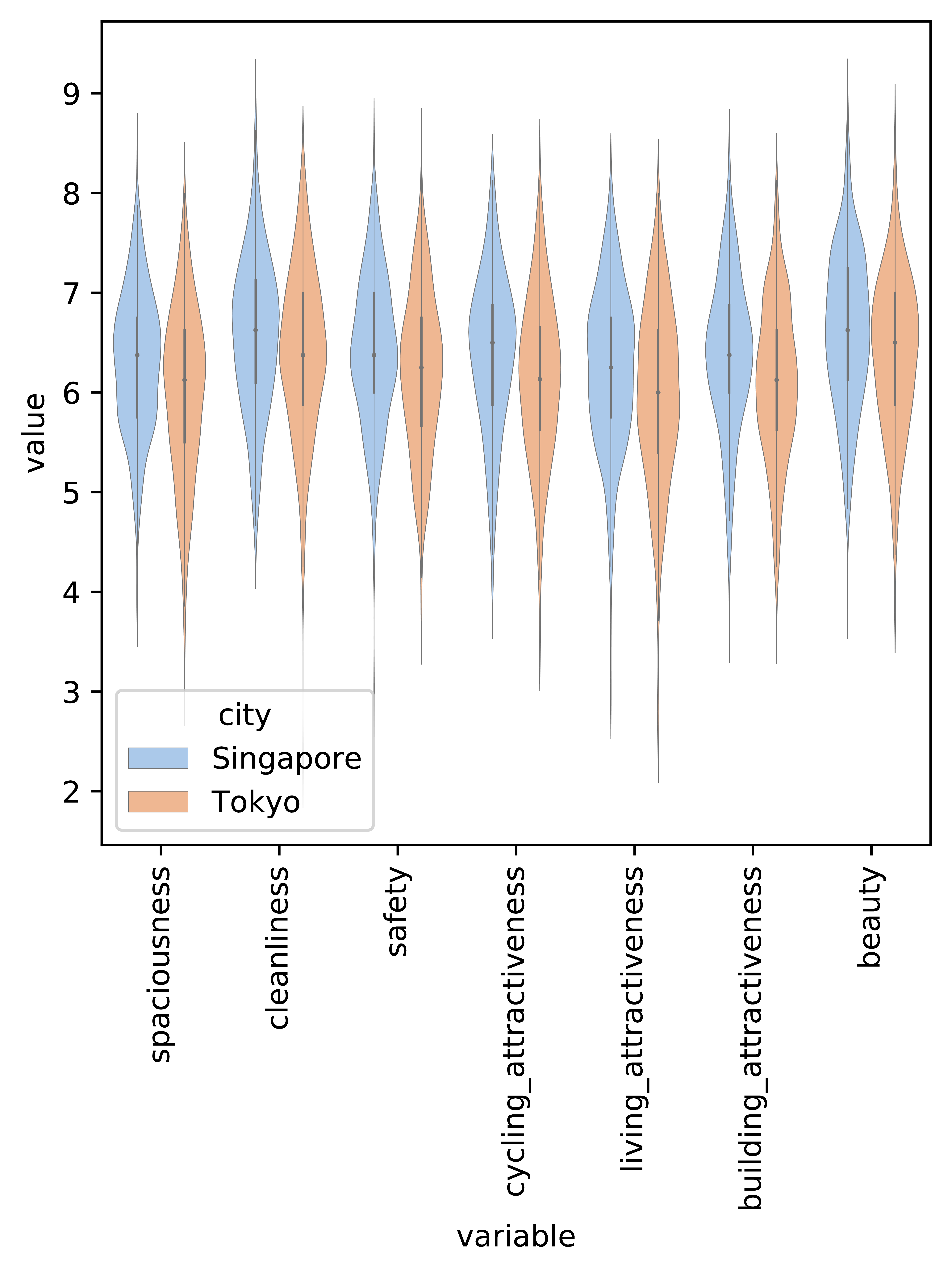
Figure 6: Distribution of seven perception scores obtained from the survey by each city.

Visual features from SVI are extracted through high-level feature extraction (i.e. semantic segmentation, classification, and object detection) and low-level feature extraction (i.e. edge detection, blob detection, and HLS statistics). After labeling each observation below or above the mean value of each feature, Welch’s t-test is conducted to find features with statistically significant effects on perception scores based on the labeling. The total number of extracted features is 519, and the number of scores is seven; therefore, there are 3,633 unique feature-score pairs.

For beauty, we found that features that contribute to better infrastructures such as curb and terrain contribute to higher scores, while features that damage beauty such as utility poles and junkyards contribute to lower scores. Also, for low-level features, larger standard deviations of HLS are associated with lower beauty scores.

As for building attractiveness, we realize that a higher pixel ratio of buildings and classification as slums leads to lower scores, implying that participants did not prefer dense buildings. On the other hand, classification as residential neighborhood and campus leads to higher scores, suggesting residential and education as potential land uses and typologies that make people feel attracted to buildings.

The result of cleanliness suggests that classification as campus and higher pixel ratio of curb leads to higher cleanliness scores, which might imply that these places and infrastructures are relatively better maintained. On the other hand, classification as junkyard and landfill led to lower cleanliness scores, which is intuitively understandable because of their strong associations with garbage. As for cycling attractiveness, natural elements such as terrain and vegetation as well as classification as residential neighborhoods leads to higher cycling attractiveness scores, while utility poles and construction sites are associated with lower scores. Attractiveness for living obtains a similar pattern to other scores. A higher pixel ratio of terrain and curb entails higher scores, and classification as slum and landfill causes lower scores. The result of safety shows that terrain and campus achieve higher scores and that other features such as gas stations, junkyards, and slums were associated with lower safety scores. Lastly, spaciousness gains higher scores when terrain, curb, and campus are present, while other features, such as utility poles, junkyards, and larger standard deviations of HLS statistics are detrimental.

In this exploratory analysis, some parts of the study by Verma et al. (2020) are replicated such as low associations among perception scores and edge detection and blob detection. However, other parts of the study such as the strong influence of cars in object detection could not be reproduced, suggesting that the geography of the study and/or training data may play a role. Moreover, more features from image classification are found to have an influence on perception scores than other features.

Based on the study by Verma et al. (2020), predictive modeling is conducted for each perception score between 0 and 10 with high- and low-level features (see Table 4). Table 5 underscores the results of the modeling with different performance metrics, where one can see low mean absolute error (MAE) around 0.65, mean absolute percentage error (MAPE) around 0.1, and root mean squared error (RMSE) around 0.8; however, all the $R^{2}$ values were below 0. This means that the models were worse than predicting the constant values regardless of input data.

Although Verma et al. (2020) achieves $R^{2}$ as high as 0.66 by using the same visual features, our study could not achieve comparable results. This discrepancy might be due to the disparate level of data quality in the SVI training set. After the modeling, we randomly selected SVI images with higher and lower scores and found that some partially grey images and indoor images were still in the set despite the efforts to clean the data prior to the modeling. Such noise in SVI data is not often discussed in previous studies using SVI, and this issue remains to be solved in the future (Biljecki and Ito, 2021). To further improve the prediction, other visual feature extractions and selection methods need to be explored as well.

Table 5: Results of predictive modeling of perception indicators.

Target_variable	MAE	MAPE	RMSE	R2
beauty	0.63	0.10	0.81	-0.20
building_attractiveness	0.63	0.10	0.78	-0.14
cleanliness	0.63	0.10	0.79	-0.12
cycling_attractiveness	0.65	0.11	0.83	-0.18
living_attractiveness	0.69	0.12	0.87	-0.10
safety	0.72	0.12	0.89	-0.29
spaciousness	0.67	0.11	0.83	-0.19

4.2.6 Bikeability

After incorporating scores across all categories, bikeability scores were calculated at a fine spatial scale (Figure 7). In Singapore, bikeability scores are generally distributed homogeneously barring a few outliers. The results for Tokyo seem to be more heterogeneous, with a lower score in the central area and peripheral areas and higher scores in between. The distribution of data indicates no skewness in the data, and a comparison between Singapore and Tokyo in Table 6 hints that Singapore achieved a slightly higher mean value and lower standard deviation than Tokyo.

This bikeability index, however, has some issues that need to be exposed. Firstly, the perception prediction’s result is not entirely reliable. Although MAE, MAPE, and RMSE of models turned out to be moderately acceptable, $R^{2}$ values resulted in negative values, indicating the models are more inaccurate than simply predicting the mean values of the scores. Low variances among observations in some categories also need to be considered. Summary statistics shown in Table 6 and data distribution shown in Figure 8 suggest some categories such as vehicle-cyclist interaction had low standard deviation and skewed data distribution with a few outliers. This poses a question regarding the appropriate indicators to be used that can differentiate bikeability scores within and between cities because most of the sample points obtain highly similar scores for such categories. This question needs to be examined by expanding study areas in different contexts to observe whether this phenomenon is simply caused by similar characteristics of streets in the Asian context.

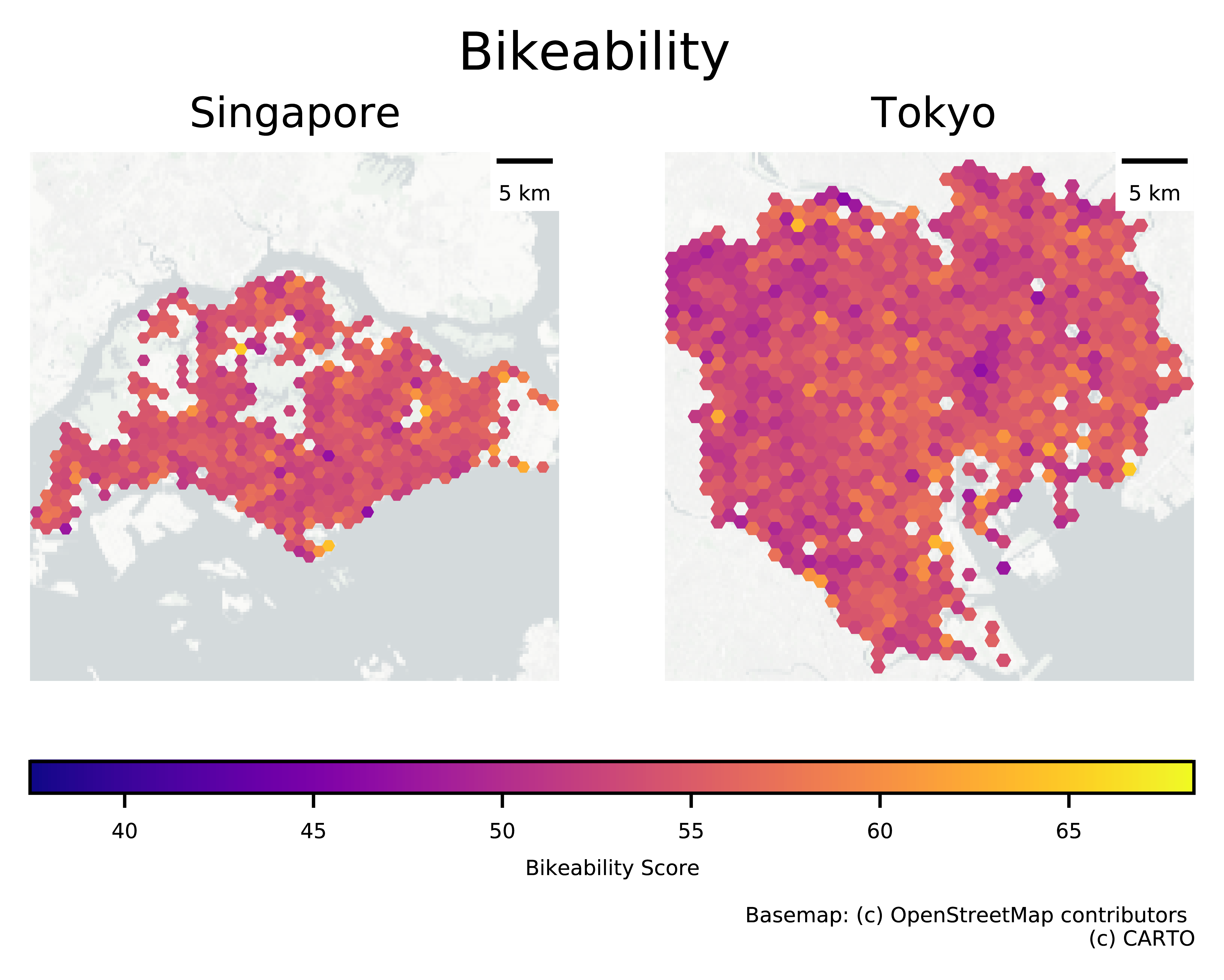
Figure 7: One of the key outputs of this study: maps of bikeability across Singapore and Tokyo, generated from the scores at numerous locations in the two cities.

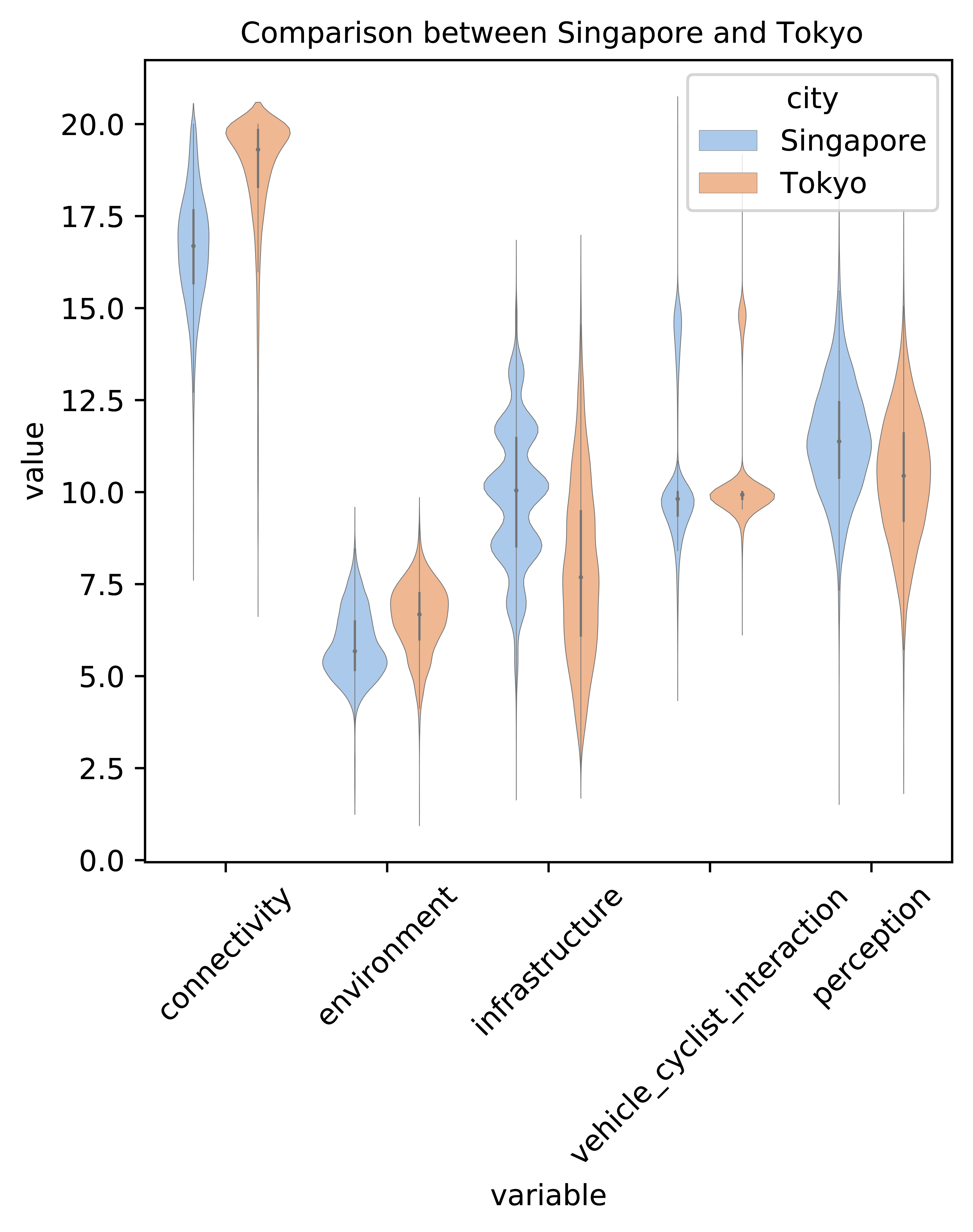
Figure 8: Distribution of scores across categories in Singapore and Tokyo.

Table 6: Summary statistics of the bikeability measures calculated for the study area.

Category	City	Mean	Standard deviation
Bikeability	Singapore	54.26	3.66
	Tokyo	53.98	3.73
Connectivity	Singapore	16.63	1.59
	Tokyo	18.72	1.70
Environment	Singapore	5.83	0.94
	Tokyo	6.58	0.94
Infrastructure	Singapore	9.88	1.90
	Tokyo	7.86	2.36
Perception	Singapore	11.42	1.57
	Tokyo	10.40	1.74
Vehicle–cyclist interaction	Singapore	10.50	2.12
	Tokyo	10.42	1.61

4.3 Comparison between SVI and Non-SVI indicators

This study compares three types of indexes to answer one of the research questions gauging the value of SVI in bikeability studies. Besides the comprehensive index developed with both SVI and non-SVI indicators, indexes with only SVI and non-SVI indicators are developed and compared with each other. Each category’s score was recalculated based on the indicator types, and, for bikeability, we compare the indexes by plotting scores developed with different indicators on the same sample points. Connectivity and perception were excluded from this analysis because these categories only had one type of indicator, only non-SVI indicators, and only SVI indicators, respectively.

Indexes of the environment developed with SVI and non-SVI indicators are not correlated with each other and that non-SVI indicators are more strongly correlated with the index developed with both of the indicators. On the other hand, SVI indicators had more influence on infrastructure and vehicle-cyclist interaction. After combining all the categories, bikeability scores were compared among different indicator types, and SVI indicators turned out to have a stronger correlation with the index with both indicator types and lower kurtosis than non-SVI indicators (see Figure 10 and Figure 10). Although this result is not a surprise given the larger number of SVI indicators than non-SVI indicators, this result indicates the potential of SVI indicators to be used alone to evaluate bikeability because of its high correlation, $R^{2}$ of 0.85, with the index with both indicators and capability to explain most of the variance.

Although it was found possible to estimate bikeability only with SVI indicators, some relevant non-SVI indicators are either difficult or impossible to replace with SVI. For example, transit facilities, POIs, and land uses are not impossible but complicated to obtain from SVI and are much more straightforward to collect from OSM and other data sources, which are anyway frequently available. Also, the slope and air quality are unnecessarily challenging to estimate from SVI, and other data sources are much less involved to collect and much more accurate than it would be if estimating them from SVI. Therefore, with these outcomes in mind, it is more beneficial for urban planners and researchers to combine both SVI and non-SVI indicators to assess bikeability, complementing the best of the two worlds.

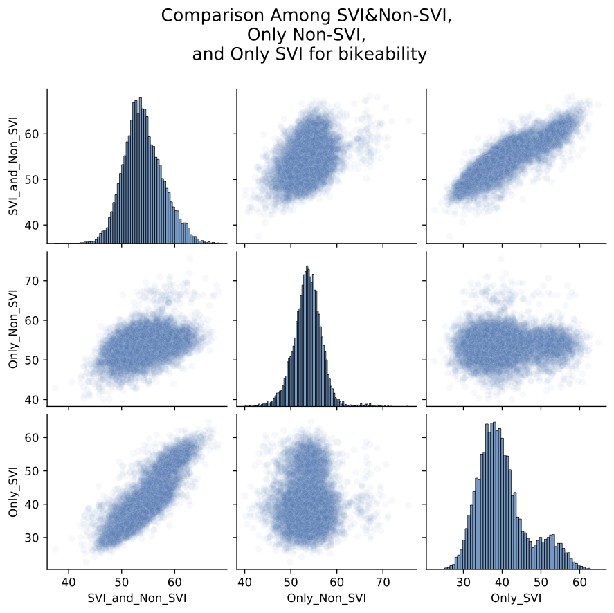
Figure 9: A scatter plot matrix of bikeability score
with only SVI and non-SVI indicators.

Figure 10: A correlation matrix of bikeability score
with only SVI and non-SVI indicators.

5 Challenges and future directions

5.1 Data quality

This study faced several challenges. One of such challenges was the quality of data. This issue surfaced in data sources, such as SVI, OSM, and AQI. GSV was used to collect SVI in this study, and the sample points of collected GSV panorama images were randomly selected to cover the entire study areas with a limited number of sample points of GSV that can be obtained for free. A study by Kim et al. (2021) reported that larger sampling intervals lead to larger variances of elements that can be extracted from SVI. Therefore, one of the limitations of this study is possible biases and larger variances of data introduced by random sampling intervals when conducting random sampling. Future studies can define shorter sampling intervals to reduce the possible bias. Another possible bias is the perspective of SVI. Because SVI is collected from vehicles, it might not always represent the typical view of bicyclists, especially for wide roads. This limitation is also faced by other previous studies on walkability that as well use 360-degree panoramas for assessment, as they aim to gauge what pedestrians perceive (Wakamiya et al., 2019; Yencha, 2019; Nagata et al., 2020; Villeneuve et al., 2018; Li et al., 2018; Zhang et al., 2018; Weld et al., 2019). In this study, the result showed that cycling paths are not highly prevalent in both Singapore and Tokyo; thus, the panorama views possibly present most of the actual cycling perspectives. Although SVI on cycling paths is not widely available currently, future studies might be able to work on SVI on cycling paths with the rise of crowdsourced SVI services, such as Mapillary.

As for OSM data, while in general of high quality for both locations, its data completeness became a bottleneck when evaluating some particular indicators (e.g. traffic speed and the number of traffic lanes) and resulted in their eliminations, so future studies should explore different data sources to collect them.

AQI data are available in both cities, but the number of AQI stations in Singapore, five, was far fewer than Tokyo, 126, and such low spatial granularity of data might have affected the result. Therefore, future studies can incorporate predictive modeling to estimate AQI for each sample point by using traffic data, meteorological data, and land use data (Chen et al., 2010).

Low variances among sample points for some indicators were found as well. This is potentially problematic because indicators with extremely low variances cannot differentiate sample points; thus, this needs to be examined more by investigating more diverse sets of cities.

Perception modeling was another challenge faced in this study due to the nature of the approach. The comprehensive survey was conducted on a service on which the majority of participants are not residents of the study areas, which may be advantageous but also detrimental. On the one hand, survey results might have been different if they were conducted with residents in the study areas (Difallah et al., 2018). To mitigate the potential bias, future studies can utilize different survey services that can specify the residence of the participants. On the other hand, having participants of a cross-city study residing in neither study area may mitigate the bias of residents living in one city but not being familiar with the other one.

5.2 Required skills

Because the data collection and processing was conducted using Python, this method requires users to have a moderately advanced understanding of programming. Computational power is also a challenge because this study’s method uses CV techniques that require graphics processing capabilities, which are not available widely. To mitigate these limitations, future studies may consider developing a GUI software and an API to allow users to input data and assess bikeability.

5.3 Development of the index

This study selected the indicators based on the systematic review. However, purposes of cycling and socio-economic characteristics might affect the indicator selection and weight assignment, as examined by Arellana et al. (2020). Moreover, a bikeability assessment based on route simulations between origin and destinations called capability-wise walkability score has been proposed by a previous study (Blečić et al., 2021). Thus, the incorporation of such new designs of bikeability index might be able to enhance our method as well.

6 Conclusion

In previous studies, it has been a challenge to make bikeability assessment scalable while keeping a good balance of objectivity and subjectivity, and minimizing the work required. The few studies that have used SVI and CV techniques to automate the process and increase the geographic coverage rather assessed limited aspects of bikeability and have not done so critically, nor have they investigated the inclusion of multiple cities.

We advanced the comprehensive assessment of bikeability using street view imagery and computer vision. The contributions of our study are the creation of an exhaustive bikeability index inspired by previous studies with SVI indicators extracted with CV techniques as the major data source, novel exploration of automatable subjective assessment of bikeability, comparison of SVI and non-SVI indicators for the first time, and a novel investigation of the potential of using SVI indicators independently for bikeability assessment.

Non-perception SVI indicators were extracted using semantic segmentation and object detection, and perception SVI indicators were predicted by training models with survey results as target variables and visual features extracted from SVI as independent variables. Bikeability indexes that range from 0 to 100 were developed in Singapore and Tokyo and compared with each other, which resulted in slightly higher bikeability scores in Singapore, 54.26 on average, than in Tokyo, 53.98 on average. A thorough comparison between SVI and non-SVI indicators was made to examine which has more influence when predicting conditions and the appeal of cycling. SVI indicators turned out to have a much stronger correlation with the estimated bikeability index, an $R^{2}$ of 0.85, outperforming non-SVI indicators, which had an $R^{2}$ of 0.4. However, the usefulness of the latter should not be discounted.

In summary, the takeaways of this research are:

• This study has demonstrated that we can use CV techniques and SVI to comprehensively assess bikeability within and among cities. The paper details the design and implementation of a bikeability index that relies on SVI and CV, which is calculated at both a fine spatial scale and aggregated at the level of a city. The study asserts that this index at least supplements traditional instruments used in this research domain.

• Indicators that are derived from SVI dwarf those that are computed from non-SVI counterparts. A large portion of the variance in the overall index was explained by SVI indicators, overshadowing those prominent in orthodox mechanisms used hitherto.

• SVI may potentially be used on its own to assess bikeability in the built environment. However, as elaborated in the previous sections, this study faced several challenges that, despite the convincing usability of SVI, may not make taking this independent route always viable. Thus, future studies need to ameliorate several practical issues. Further, the comparative advantage comes at a price — it is more difficult to obtain SVI indicators in comparison to the non-SVI counterparts. Therefore, despite the relative usability and independence of either, it might be beneficial to use both to assess bikeability, complementing their pros and cons.

Based on the findings from this study, future research should focus not only on overcoming the challenges discussed in the previous section but also on further enhancing the index, which advances the state of the art but may nevertheless benefit from further work. The index can be improved by expanding the scope of SVI indicators to be included and also improving the indicator weights according to cyclists’ preferences. The enlargement of the indicators can be done by building CV models to extract more indicators, such as road type, land use, and type of pavement. Some studies have explored creating weights based on cyclists’ preferences through surveys, creating different weights for different types of cyclists (Arellana et al., 2020). Such improvement of the weights can benefit better decision-making in urban planning according to the demographics in target areas, thus, future studies should also incorporate such methods. Another direction for future work would be coupling the developed index with instances introduced to assess other urban aspects such as walkability and livability (Zhao et al., 2020; Benita et al., 2020), to investigate relationships or complement them.

List of acronyms

AQI	Air Quality Index
CV	Computer Vision
DEM	Digital Elevation Model
HSL	Hue-Saturation-Lightness
IC	Image Classification
LU	Land Use
MAE	Mean Absolute Error
MAPE	Mean Absolute Percentage Error
GSV	Google Street View
OD	Object Detection
OSM	OpenStreetMap
POI	Point of Interest
RMSE	Root Mean Squared Error
SS	Semantic Segmentation
SVI	Street View Imagery
V–C Interaction	Vehicle–Cyclist Interaction

References

- Abadi and Hurwitz (2018) Abadi, M.G., Hurwitz, D.S., 2018. Bicyclist’s perceived level of comfort in dense urban environments: How do ambient traffic, engineering treatments, and bicyclist characteristics relate? Sustainable Cities and Society 40, 101–109. doi:10.1016/j.scs.2018.04.003.
- Alaoui and Tekouabou (2021) Alaoui, E.A.A., Tekouabou, S.C.K., 2021. Intelligent management of bike sharing in smart cities using machine learning and internet of things. Sustainable Cities and Society 67, 102702. doi:10.1016/j.scs.2020.102702.
- Aldred et al. (2020) Aldred, R., García-Herrero, S., Anaya, E., Herrera, S., Mariscal, M., 2020. Cyclist injury severity in spain: A bayesian analysis of police road injury data focusing on involved vehicles and route environment. International Journal of Environmental Research and Public Health 17. doi:10.3390/ijerph17010096.
- Arellana et al. (2020) Arellana, J., Saltarín, M., Larrañaga, A.M., González, V.I., Henao, C.A., 2020. Developing an urban bikeability index for different types of cyclists as a tool to prioritise bicycle infrastructure investments. Transportation Research Part A: Policy and Practice 139, 310–334. doi:10.1016/j.tra.2020.07.010.
- Attard et al. (2021) Attard, M., Cañas, C., Maas, S., 2021. Determinants for walking and cycling to a university campus: Insights from a participatory Active Travel workshop in Malta. Transportation Research Procedia 52, 501–508. doi:10.1016/j.trpro.2021.01.059.
- Barrington-Leigh and Millard-Ball (2017) Barrington-Leigh, C., Millard-Ball, A., 2017. The world’s user-generated road map is more than 80% complete. PLOS ONE 12, e0180698 – 20. doi:10.1371/journal.pone.0180698.
- Barter (2010) Barter, P.A., 2010. Parking Policy in Asian Cities. SSRN Electronic Journal URL: http://www.ssrn.com/abstract=1780012, doi:10.2139/ssrn.1780012.
- Bauman et al. (2012) Bauman, A.E., Reis, R.S., Sallis, J.F., Wells, J.C., Loos, R.J., Martin, B.W., 2012. Correlates of physical activity: why are some people physically active and others not? The Lancet 380, 258–271. doi:10.1016/s0140-6736(12)60735-1.
- Benita et al. (2020) Benita, F., Kalashnikov, V., Tunçer, B., 2020. A Spatial Livability Index for dense urban centers. Environment and Planning B: Urban Analytics and City Science , 239980832096015doi:10.1177/2399808320960151.
- Berger and Dörrzapf (2018) Berger, M., Dörrzapf, L., 2018. Sensing comfort in bicycling in addition to travel data, pp. 524–534. doi:10.1016/j.trpro.2018.10.034.
- Biljecki (2020) Biljecki, F., 2020. Exploration of open data in Southeast Asia to generate 3D building models. ISPRS Annals of Photogrammetry, Remote Sensing and Spatial Information Sciences VI-4/W1-2020, 37–44. doi:10.5194/isprs-annals-vi-4-w1-2020-37-2020.
- Biljecki and Ito (2021) Biljecki, F., Ito, K., 2021. Street view imagery in urban analytics and GIS: A review. Landscape and Urban Planning 215, 104217. doi:10.1016/j.landurbplan.2021.104217.
- Blečić et al. (2021) Blečić, I., Cecchini, A., Congiu, T., Fancello, G., Talu, V., Trunfio, G.A., 2021. Capability-wise walkability evaluation as an indicator of urban peripherality. Environment and Planning B: Urban Analytics and City Science 48, 895–911. URL: https://doi.org/10.1177/2399808320908294, doi:10.1177/2399808320908294. publisher: SAGE Publications Ltd STM.
- Boeing (2017) Boeing, G., 2017. OSMnx: New methods for acquiring, constructing, analyzing, and visualizing complex street networks. Computers, Environment and Urban Systems 65, 126–139. doi:10.1016/j.compenvurbsys.2017.05.004.
- Boongaling et al. (2021) Boongaling, C.G.K., Luna, D.A., Samantela, S.S., 2021. Developing a street level walkability index in the Philippines using 3D photogrammetry modeling from drone surveys. GeoJournal URL: https://doi.org/10.1007/s10708-021-10441-2, doi:10.1007/s10708-021-10441-2.
- Brüchert et al. (2020) Brüchert, T., Hasselder, P., Quentin, P., Bolte, G., 2020. Walking for transport among older adults: A cross-sectional study on the role of the built environment in less densely populated areas in northern germany. International Journal of Environmental Research and Public Health 17, 1–22. doi:10.3390/ijerph17249479.
- Bulò et al. (2018) Bulò, S.R., Porzi, L., Kontschieder, P., 2018. In-Place Activated BatchNorm for Memory-Optimized Training of DNNs. arXiv:1712.02616 URL: http://arxiv.org/abs/1712.02616.
- Cain et al. (2018) Cain, K.L., Geremia, C.M., Conway, T.L., Frank, L.D., Chapman, J.E., Fox, E.H., Timperio, A., Veitch, J., Van Dyck, D., Verhoeven, H., Reis, R., Augusto, A., Cerin, E., Mellecker, R.R., Queralt, A., Molina-García, J., Sallis, J.F., 2018. Development and reliability of a streetscape observation instrument for international use: MAPS-global. The International Journal of Behavioral Nutrition and Physical Activity 15, 19. doi:10.1186/s12966-018-0650-z.
- Cao and Shen (2019) Cao, Y., Shen, D., 2019. Contribution of shared bikes to carbon dioxide emission reduction and the economy in Beijing. Sustainable Cities and Society 51, 101749. doi:10.1016/j.scs.2019.101749.
- Castañon and Ribeiro (2021) Castañon, U.N., Ribeiro, P.J.G., 2021. Bikeability and Emerging Phenomena in Cycling: Exploratory Analysis and Review. Sustainability 13, 2394. doi:10.3390/su13042394.
- Chacra and Zelek (2018) Chacra, D.A., Zelek, J., 2018. Municipal Infrastructure Anomaly and Defect Detection, in: 26th European Signal Processing Conference (EUSIPCO), pp. 2125–2129. doi:10.23919/EUSIPCO.2018.8553322.
- Chen et al. (2021a) Chen, J., Stouffs, R., Biljecki, F., 2021a. Hierarchical (Multi-Label) Architectural Image Recognition and Classification, in: Proceedings of the 26th International Conference of the Association for Computer-Aided Architectural Design Research in Asia (CAADRIA) 2021, pp. 161–170.
- Chen et al. (2010) Chen, L., Bai, Z., Kong, S., Han, B., You, Y., Ding, X., Du, S., Liu, A., 2010. A land use regression for predicting NO2 and PM10 concentrations in different seasons in Tianjin region, China. Journal of Environmental Sciences 22, 1364–1373. doi:https://doi.org/10.1016/S1001-0742(09)60263-1.
- Chen et al. (2020a) Chen, L., Lu, Y., Sheng, Q., Ye, Y., Wang, R., Liu, Y., 2020a. Estimating pedestrian volume using Street View images: A large-scale validation test. Computers, Environment and Urban Systems 81, 101481. doi:10.1016/j.compenvurbsys.2020.101481.
- Chen et al. (2020b) Chen, W., Liu, Q., Zhang, C., Mi, Z., Zhu, D., Liu, G., 2020b. Characterizing the stocks, flows, and carbon impact of dockless sharing bikes in china. Resources, Conservation and Recycling 162. doi:10.1016/j.resconrec.2020.105038.
- Chen et al. (2021b) Chen, W., Wu, A.N., Biljecki, F., 2021b. Classification of urban morphology with deep learning: Application on urban vitality. Computers, Environment and Urban Systems 90, 101706. doi:10.1016/j.compenvurbsys.2021.101706.
- Chevalier and Xu (2020) Chevalier, A., Xu, L., 2020. On the applicability of a western bikeability index in the chinese context. International Review for Spatial Planning and Sustainable Development 8, 59–93. doi:10.14246/IRSPSD.8.1_59.
- Cicchino et al. (2020) Cicchino, J.B., McCarthy, M.L., Newgard, C.D., Wall, S.P., DiMaggio, C.J., Kulie, P.E., Arnold, B.N., Zuby, D.S., 2020. Not all protected bike lanes are the same: Infrastructure and risk of cyclist collisions and falls leading to emergency department visits in three U.S. cities. Accident Analysis & Prevention 141, 105490. doi:10.1016/j.aap.2020.105490.
- Clifton et al. (2007) Clifton, K.J., Livi Smith, A.D., Rodriguez, D., 2007. The development and testing of an audit for the pedestrian environment. Landscape and Urban Planning 80, 95–110. doi:10.1016/j.landurbplan.2006.06.008.
- Cordts et al. (2016) Cordts, M., Omran, M., Ramos, S., Rehfeld, T., Enzweiler, M., Benenson, R., Franke, U., Roth, S., Schiele, B., 2016. The Cityscapes Dataset for Semantic Urban Scene Understanding. arXiv:1604.01685 URL: http://arxiv.org/abs/1604.01685.
- Daraei et al. (2021) Daraei, S., Pelechrinis, K., Quercia, D., 2021. A data-driven approach for assessing biking safety in cities. EPJ Data Science 10, 1–16. doi:10.1140/epjds/s13688-021-00265-y.
- Delacre et al. (2017) Delacre, M., Lakens, D., Leys, C., 2017. Why Psychologists Should by Default Use Welch’s t-test Instead of Student’s t-test. International Review of Social Psychology 30, 92–101. doi:10.5334/irsp.82.
- Deng et al. (2018) Deng, L., Pan, J., Xu, X., Yang, W., Liu, C., Liu, H., 2018. PDRLGB: Precise DNA-binding residue prediction using a light gradient boosting machine. BMC Bioinformatics 19. doi:10.1186/s12859-018-2527-1.
- Difallah et al. (2018) Difallah, D., Filatova, E., Ipeirotis, P., 2018. Demographics and Dynamics of Mechanical Turk Workers, in: Proceedings of the Eleventh ACM International Conference on Web Search and Data Mining, ACM, Marina Del Rey CA USA. pp. 135–143. doi:10.1145/3159652.3159661.
- Ding et al. (2021) Ding, X., Fan, H., Gong, J., 2021. Towards generating network of bikeways from Mapillary data. Computers, Environment and Urban Systems 88, 101632. doi:10.1016/j.compenvurbsys.2021.101632.
- Doubleday et al. (2021) Doubleday, A., Choe, Y., Isaksen, T., Miles, S., Errett, N., 2021. How did outdoor biking and walking change during COVID-19?: A case study of three U.S. cities. PLoS ONE 16. doi:10.1371/journal.pone.0245514.
- Du et al. (2019) Du, Y., Deng, F., Liao, F., 2019. A model framework for discovering the spatio-temporal usage patterns of public free-floating bike-sharing system. Transportation Research Part C: Emerging Technologies 103, 39–55. doi:10.1016/j.trc.2019.04.006.
- Dubey et al. (2016) Dubey, A., Naik, N., Parikh, D., Raskar, R., Hidalgo, C.A., 2016. Deep Learning the City: Quantifying Urban Perception at a Global Scale, in: Leibe, B., Matas, J., Sebe, N., Welling, M. (Eds.), Computer Vision – ECCV 2016, Springer International Publishing, Cham. pp. 196–212. doi:10.1007/978-3-319-46448-0_12.
- Faghih Imani et al. (2019) Faghih Imani, A., Miller, E.J., Saxe, S., 2019. Cycle accessibility and level of traffic stress: A case study of Toronto. Journal of Transport Geography 80, 102496. URL: https://www.sciencedirect.com/science/article/pii/S0966692319300936, doi:10.1016/j.jtrangeo.2019.102496.
- Fan et al. (2021) Fan, H., Kong, G., Zhang, C., 2021. An Interactive platform for low-cost 3D building modeling from VGI data using convolutional neural network. Big Earth Data 5, 49–65. doi:10.1080/20964471.2021.1886391.
- Feng et al. (2021) Feng, G., Zou, G., Piga, B.E.A., Hu, H., 2021. The Validity of Street View Service Applied to Ambiance Perception of Street: A Comparison of Assessment in Real Site and Baidu Street View, in: Shin, C.S., Di Bucchianico, G., Fukuda, S., Ghim, Y.G., Montagna, G., Carvalho, C. (Eds.), Advances in Industrial Design, Springer International Publishing, Cham. pp. 740–748. doi:10.1007/978-3-030-80829-7_91.
- Frank et al. (2005) Frank, L.D., Schmid, T.L., Sallis, J.F., Chapman, J., Saelens, B.E., 2005. Linking objectively measured physical activity with objectively measured urban form: findings from SMARTRAQ. American Journal of Preventive Medicine 28, 117–125. doi:10.1016/j.amepre.2004.11.001.
- Galanis et al. (2018) Galanis, A., Papanikolaou, A., Eliou, N., 2018. Bikeability audit in urban road environment: Case study in the city of Volos, Greece. doi:10.4018/978-1-5225-5210-9.ch021.
- Gholamialam and Matisziw (2019) Gholamialam, A., Matisziw, T., 2019. Modeling bikeability of urban systems. Geographical Analysis 51, 73–89. doi:10.1111/gean.12159.
- Goel et al. (2018) Goel, R., Garcia, L.M.T., Goodman, A., Johnson, R., Aldred, R., Murugesan, M., Brage, S., Bhalla, K., Woodcock, J., 2018. Estimating city-level travel patterns using street imagery: A case study of using Google Street View in Britain. PLOS ONE 13, e0196521. doi:10.1371/journal.pone.0196521.
- Gong et al. (2018) Gong, F.Y., Zeng, Z.C., Zhang, F., Li, X., Ng, E., Norford, L.K., 2018. Mapping sky, tree, and building view factors of street canyons in a high-density urban environment. Building and Environment 134, 155–167. doi:10.1016/j.buildenv.2018.02.042.
- Gong et al. (2019) Gong, Z., Ma, Q., Kan, C., Qi, Q., 2019. Classifying Street Spaces with Street View Images for a Spatial Indicator of Urban Functions. Sustainability 11, 6424. doi:10.3390/su11226424.
- Google (2018) Google, 2018. "Street View ready (pro grade)" specifications. URL: https://developers.google.com/streetview/ready/specs-prograde.
- Grigore et al. (2019) Grigore, E., Garrick, N., Fuhrer, R., Axhausen, I., 2019. Bikeability in Basel. Transportation Research Record 2673, 607–617. doi:10.1177/0361198119839982.
- Gu et al. (2018) Gu, P., Han, Z., Cao, Z., Chen, Y., Jiang, Y., 2018. Using Open Source Data to Measure Street Walkability and Bikeability in China: A Case of Four Cities. Transportation Research Record 2672, 63–75. doi:10.1177/0361198118758652.
- Guler and Yomralioglu (2021) Guler, D., Yomralioglu, T., 2021. Location Evaluation of Bicycle Sharing System Stations and Cycling Infrastructures with Best Worst Method Using GIS. The Professional Geographer , 1–18doi:10.1080/00330124.2021.1883446.
- Gullón et al. (2015) Gullón, P., Badland, H.M., Alfayate, S., Bilal, U., Escobar, F., Cebrecos, A., Diez, J., Franco, M., 2015. Assessing Walking and Cycling Environments in the Streets of Madrid: Comparing On-Field and Virtual Audits. Journal of Urban Health: Bulletin of the New York Academy of Medicine 92, 923–939. doi:10.1007/s11524-015-9982-z.
- Guo et al. (2020) Guo, J., He, H., He, T., Lausen, L., Li, M., Lin, H., Shi, X., Wang, C., Xie, J., Zha, S., Zhang, A., Zhang, H., Zhang, Z., Zhang, Z., Zheng, S., Zhu, Y., 2020. GluonCV and GluonNLP: Deep Learning in Computer Vision and Natural Language Processing. arXiv:1907.04433 URL: http://arxiv.org/abs/1907.04433.
- Hall et al. (2018) Hall, P., Lu, Y., Lu, J., Zhang, S., 2018. Traffic signal detection and classification in street views using an attention model. Computational Visual Media 4, 253–266. doi:10.1007/s41095-018-0116-x.
- Han (2017) Han, H., 2017. Singapore, a Garden City: Authoritarian Environmentalism in a Developmental State. The Journal of Environment & Development 26, 3–24. doi:10.1177/1070496516677365.
- Hartanto et al. (2017) Hartanto, K., Grigolon, A.B., Maarseveen, M., Brussel, M., 2017. Developing a bikeability index in the context of transit-oriented development (TOD)., in: 15th International Conference on Computers in Urban Planning and Urban Management (CUPUM), Adelaide, Australia.
- Hoedl et al. (2010) Hoedl, S., Titze, S., Oja, P., 2010. The bikeability and walkability evaluation table reliability and application. American Journal of Preventive Medicine 39, 457–459. doi:10.1016/j.amepre.2010.07.005.
- Hollander et al. (2020) Hollander, J.B., Nikolaishvili, G., Adu-Bredu, A.A., Situ, M., Bista, S., 2020. Using deep learning to examine the correlation between transportation planning and perceived safety of the built environment. Environment and Planning B: Urban Analytics and City Science , 2399808320959079doi:10.1177/2399808320959079.
- Horacek et al. (2018) Horacek, T., Dede Yildirim, E., Kattelmann, K., Brown, O., Byrd-Bredbenner, C., Colby, S., Greene, G., Hoerr, S., Kidd, T., Koenings, M., Morrell, J., Olfert, M., Phillips, B., Shelnutt, K., White, A., 2018. Path analysis of campus walkability/bikeability and college students’ physical activity attitudes, behaviors, and body mass index. American Journal of Health Promotion 32, 578–586. doi:10.1177/0890117116666357.
- Horacek et al. (2012) Horacek, T.M., White, A.A., Greene, G.W., Reznar, M.M., Quick, V.M., Morrell, J.S., Colby, S.M., Kattelmann, K.K., Herrick, M.S., Shelnutt, K.P., Mathews, A., Phillips, B.W., Byrd-Bredbenner, C., 2012. Sneakers and spokes: An assessment of the walkability and bikeability of U.S. postsecondary institutions. Journal of Environmental Health 74, 8–15.
- Inajima and Urabe (2017) Inajima, T., Urabe, E., 2017. Koike’s plan for Tepco to remove utility poles in Tokyo an Olympian task. URL: https://www.japantimes.co.jp/news/2017/04/03/business/koikes-plan-tepco-remove-utility-poles-tokyo-olympian-task/.
- Kalvelage et al. (2018) Kalvelage, K., Kalvelage, K., Dorneich, M.C., Dorneich, M.C., Seeger, C.J., Seeger, C.J., Welk, G.J., Welk, G.J., Gilbert, S., Gilbert, S., Moon, J., Moon, J., Jafir, I., Jafir, I., Brown, P., Brown, P., 2018. Assessing the validity of facilitated-volunteered geographic information: comparisons of expert and novice ratings. GeoJournal 83, 477–488. doi:10.1007/s10708-017-9781-z.
- Kamel et al. (2020) Kamel, M., Sayed, T., Bigazzi, A., 2020. A composite zonal index for biking attractiveness and safety. Accident Analysis and Prevention 137. doi:10.1016/j.aap.2020.105439.
- Kang et al. (2019) Kang, H., Kim, D., Yoo, S., 2019. Attributes of perceived bikeability in a compact urban neighborhood based on qualitative multi-methods. International Journal of Environmental Research and Public Health 16. doi:10.3390/ijerph16193738.
- Kang et al. (2021) Kang, Y., Zhang, F., Gao, S., Peng, W., Ratti, C., 2021. Human settlement value assessment from a place perspective: Considering human dynamics and perceptions in house price modeling. Cities 118, 103333. URL: https://www.sciencedirect.com/science/article/pii/S026427512100233X, doi:10.1016/j.cities.2021.103333.
- Ke et al. (2017) Ke, G., Meng, Q., Finley, T., Wang, T., Chen, W., Ma, W., Ye, Q., Liu, T.Y., 2017. LightGBM: a highly efficient gradient boosting decision tree, in: Proceedings of the 31st International Conference on Neural Information Processing Systems, Curran Associates Inc., Red Hook, NY, USA. pp. 3149–3157.
- Kellstedt et al. (2021) Kellstedt, D.K., Spengler, J.O., Foster, M., Lee, C., Maddock, J.E., 2021. A Scoping Review of Bikeability Assessment Methods. Journal of Community Health 46, 211–224. doi:10.1007/s10900-020-00846-4.
- Kim et al. (2021) Kim, J.H., Lee, S., Hipp, J.R., Ki, D., 2021. Decoding urban landscapes: Google street view and measurement sensitivity. Computers, Environment and Urban Systems 88, 101626. doi:10.1016/j.compenvurbsys.2021.101626.
- Koh and Wong (2013) Koh, P.P., Wong, Y., 2013. Influence of infrastructural compatibility factors on walking and cycling route choices. Journal of Environmental Psychology 36, 202–213. doi:10.1016/j.jenvp.2013.08.001.
- Kraus and Koch (2021) Kraus, S., Koch, N., 2021. Provisional COVID-19 infrastructure induces large, rapid increases in cycling. Proceedings of the National Academy of Sciences 118. doi:10.1073/pnas.2024399118.
- Krenn et al. (2015) Krenn, P.J., Oja, P., Titze, S., 2015. Development of a Bikeability Index to Assess the Bicycle-Friendliness of Urban Environments. Open Journal of Civil Engineering 05, 451. doi:10.4236/ojce.2015.54045.
- Labetski and Chum (2020) Labetski, A., Chum, A., 2020. Built environmental correlates of cycling accidents involving fatalities and serious injuries in london, uk. Frontiers in Sustainable Cities 2, 59. doi:10.3389/frsc.2020.599635.
- Li et al. (2020) Li, M., Zhang, Z., Lei, L., Wang, X., Guo, X., 2020. Agricultural Greenhouses Detection in High-Resolution Satellite Images Based on Convolutional Neural Networks: Comparison of Faster R-CNN, YOLO v3 and SSD. Sensors 20, 4938. URL: https://www.mdpi.com/1424-8220/20/17/4938, doi:10.3390/s20174938.
- Li and Ratti (2019) Li, X., Ratti, C., 2019. Using Google Street View for Street-Level Urban Form Analysis, a Case Study in Cambridge, Massachusetts, in: D’Acci, L. (Ed.), The Mathematics of Urban Morphology. Springer International Publishing, pp. 457–470. doi:10.1007/978-3-030-12381-9_20.
- Li et al. (2018) Li, X., Santi, P., Courtney, T.K., Verma, S.K., Ratti, C., 2018. Investigating the association between streetscapes and human walking activities using Google Street View and human trajectory data. Transactions in GIS 22, 1029–1044. URL: http://onlinelibrary.wiley.com/doi/abs/10.1111/tgis.12472, doi:10.1111/tgis.12472. _eprint: https://onlinelibrary.wiley.com/doi/pdf/10.1111/tgis.12472.
- Li et al. (2017) Li, X.j., Ratti, C., Seiferling, I., 2017. Quantifying the shade provision of street trees in urban landscape: A case study in Boston, USA, using Google Street View. Landscape and Planning 169. doi:10.1016/j.landurbplan.2017.08.011.
- Lin and Wei (2018) Lin, J.J., Wei, Y.H., 2018. Assessing area-wide bikeability: A grey analytic network process. Transportation Research Part A: Policy and Practice 113, 381–396. doi:10.1016/j.tra.2018.04.022.
- Long and Zhao (2020) Long, Y., Zhao, J., 2020. What makes a city bikeable? a study of intercity and intracity patterns of bicycle ridership using mobike big data records. Built Environment 46, 55–75. doi:10.2148/benv.46.1.55.
- Lowry et al. (2016) Lowry, M.B., Furth, P., Hadden-Loh, T., 2016. Low-Stress Neighborhood Bikeability Assessment to Prioritize Bicycle Infrastructure. URL: https://trid.trb.org/view/1392413. number: 16-1115.
- Lu (2019) Lu, Y., 2019. Using Google Street View to investigate the association between street greenery and physical activity. Landscape and Urban Planning 191, 103435. doi:10.1016/j.landurbplan.2018.08.029.
- Lu et al. (2019) Lu, Y., Yang, Y., Sun, G., Gou, Z., 2019. Associations between overhead-view and eye-level urban greenness and cycling behaviors. Cities 88, 10–18. doi:10.1016/j.cities.2019.01.003.
- Luo et al. (2020) Luo, H., Zhao, F., Chen, W.Q., Cai, H., 2020. Optimizing bike sharing systems from the life cycle greenhouse gas emissions perspective. Transportation Research Part C: Emerging Technologies 117, 102705. doi:10.1016/j.trc.2020.102705.
- Ma and Dill (2017) Ma, L., Dill, J., 2017. Do people’s perceptions of neighborhood bikeability match "reality"? Journal of Transport and Land Use 10, 291–308.
- Ma et al. (2021) Ma, X., Ma, C., Wu, C., Xi, Y., Yang, R., Peng, N., Zhang, C., Ren, F., 2021. Measuring human perceptions of streetscapes to better inform urban renewal: A perspective of scene semantic parsing. Cities 110, 103086. doi:10.1016/j.cities.2020.103086.
- Manton et al. (2016) Manton, R., Rau, H., Fahy, F., Sheahan, J., Clifford, E., 2016. Using mental mapping to unpack perceived cycling risk. Accident Analysis & Prevention 88, 138–149. doi:10.1016/j.aap.2015.12.017.
- Martin et al. (2021) Martin, A., Morciano, M., Suhrcke, M., 2021. Determinants of bicycle commuting and the effect of bicycle infrastructure investment in london: Evidence from uk census microdata. Economics and Human Biology 41. doi:10.1016/j.ehb.2020.100945.
- McNeil (2011) McNeil, N., 2011. Bikeability and the 20-min Neighborhood: How Infrastructure and Destinations Influence Bicycle Accessibility. Transportation Research Record 2247, 53–63. doi:10.3141/2247-07.
- Munira et al. (2021) Munira, S., Sener, I.N., Zhang, Y., 2021. Estimating Bicycle Demand in the Austin, Texas Area: Role of a Bikeability Index. Journal of Urban Planning and Development 147, 04021036. URL: http://ascelibrary.org/doi/abs/10.1061/%28ASCE%29UP.1943-5444.0000725, doi:10.1061/(ASCE)UP.1943-5444.0000725. publisher: American Society of Civil Engineers.
- Nagata et al. (2020) Nagata, S., Nakaya, T., Hanibuchi, T., Amagasa, S., Kikuchi, H., Inoue, S., 2020. Objective scoring of streetscape walkability related to leisure walking: Statistical modeling approach with semantic segmentation of Google Street View images. Health & Place 66, 102428. doi:10.1016/j.healthplace.2020.102428.
- Naik et al. (2014) Naik, N., Philipoom, J., Raskar, R., Hidalgo, C., 2014. Streetscore – Predicting the Perceived Safety of One Million Streetscapes. MIT web domain URL: https://dspace.mit.edu/handle/1721.1/92811.
- Najafizadeh and Froehlich (2018) Najafizadeh, L., Froehlich, J.E., 2018. A Feasibility Study of Using Google Street View and Computer Vision to Track the Evolution of Urban Accessibility, in: Proceedings of the 20th International ACM SIGACCESS Conference on Computers and Accessibility, Association for Computing Machinery, New York, NY, USA. pp. 340–342. doi:10.1145/3234695.3240999.
- Nazemi et al. (2021) Nazemi, M., van Eggermond, M.A.B., Erath, A., Schaffner, D., Joos, M., Axhausen, K.W., 2021. Studying bicyclists’ perceived level of safety using a bicycle simulator combined with immersive virtual reality. Accident Analysis & Prevention 151, 105943. doi:10.1016/j.aap.2020.105943.
- Neuhold et al. (2017) Neuhold, G., Ollmann, T., Bulo, S.R., Kontschieder, P., 2017. The Mapillary Vistas Dataset for Semantic Understanding of Street Scenes, in: 2017 IEEE International Conference on Computer Vision (ICCV), IEEE, Venice. pp. 5000–5009. doi:10.1109/ICCV.2017.534.
- Neves and Brand (2019) Neves, A., Brand, C., 2019. Assessing the potential for carbon emissions savings from replacing short car trips with walking and cycling using a mixed GPS-travel diary approach. Transportation Research Part A: Policy and Practice 123, 130–146. doi:10.1016/j.tra.2018.08.022.
- Nielsen and Skov-Petersen (2018) Nielsen, T., Skov-Petersen, H., 2018. Bikeability – urban structures supporting cycling. effects of local, urban and regional scale urban form factors on cycling from home and workplace locations in denmark. Journal of Transport Geography 69, 36–44. doi:10.1016/j.jtrangeo.2018.04.015.
- Nogal and Jiménez (2020) Nogal, M., Jiménez, P., 2020. Attractiveness of bike-sharing stations from a multi-modal perspective: The role of objective and subjective features. Sustainability 12, 1–26. doi:10.3390/su12219062.
- Osama et al. (2020) Osama, A., Albitar, M., Sayed, T., Bigazzi, A., 2020. Determining if walkability and bikeability indices reflect pedestrian and cyclist safety. Transportation Research Record 2674, 767–775. doi:10.1177/0361198120931844.
- Palliwal et al. (2021) Palliwal, A., Song, S., Tan, H.T.W., Biljecki, F., 2021. 3D city models for urban farming site identification in buildings. Computers, Environment and Urban Systems 86, 101584. doi:10.1016/j.compenvurbsys.2020.101584.
- Porter et al. (2018) Porter, A., Kohl, H., Pérez, A., Reininger, B., Gabriel, K., Salvo, D., 2018. Perceived social and built environment correlates of transportation and recreation- only bicycling among adults. Preventing Chronic Disease 15. doi:10.5888/pcd15.180060.
- Porter et al. (2020) Porter, A.K., Kohl, H.W., Pérez, A., Reininger, B., Pettee Gabriel, K., Salvo, D., 2020. Bikeability: Assessing the Objectively Measured Environment in Relation to Recreation and Transportation Bicycling. Environment and Behavior 52, 861–894. doi:10.1177/0013916518825289.
- Pritchard et al. (2019) Pritchard, R., Frøyen, Y., Snizek, B., 2019. Bicycle level of service for route choice—A GIS evaluation of four existing indicators with empirical data. ISPRS International Journal of Geo-Information 8. doi:10.3390/ijgi8050214.
- Qiu et al. (2021) Qiu, W., Li, W., Liu, X., Huang, X., 2021. Subjectively Measured Streetscape Perceptions to Inform Urban Design Strategies for Shanghai. ISPRS International Journal of Geo-Information 10, 493. URL: https://www.mdpi.com/2220-9964/10/8/493, doi:10.3390/ijgi10080493. number: 8 Publisher: Multidisciplinary Digital Publishing Institute.
- Resch et al. (2020) Resch, B., Puetz, I., Bluemke, M., Kyriakou, K., Miksch, J., 2020. An interdisciplinary mixed-methods approach to analyzing urban spaces: The case of urban walkability and bikeability. International Journal of Environmental Research and Public Health 17, 1–20. doi:10.3390/ijerph17196994.
- Rojas-Rueda et al. (2011) Rojas-Rueda, D., Nazelle, A.d., Tainio, M., Nieuwenhuijsen, M.J., 2011. The health risks and benefits of cycling in urban environments compared with car use: health impact assessment study. BMJ 343, d4521. doi:10.1136/bmj.d4521.
- Russo et al. (2019) Russo, A., Ommeren, J.v., Dimitropoulos, A., 2019. The environmental and welfare implications of parking policies. doi:10.1787/16d610cc-en.
- Schmid-Querg et al. (2021) Schmid-Querg, J., Keler, A., Grigoropoulos, G., 2021. The Munich Bikeability Index: A Practical Approach for Measuring Urban Bikeability. Sustainability 13, 1–14. doi:10.3390/su13010428.
- Singapore Government (2020a) Singapore Government, 2020a. Annual Motor Vehicle Population by Vehicle Type. URL: https://data.gov.sg/dataset/annual-motor-vehicle-population-by-vehicle-type.
- Singapore Government (2020b) Singapore Government, 2020b. Master Plan 2019 Land Use layer. URL: https://data.gov.sg/dataset/master-plan-2019-land-use-layer.
- Song et al. (2020) Song, X.P., Richards, D.R., Tan, P.Y., 2020. Using social media user attributes to understand human–environment interactions at urban parks. Scientific Reports 10, 808. doi:10.1038/s41598-020-57864-4.
- Sottile et al. (2019) Sottile, E., Sanjust di Teulada, B., Meloni, I., Cherchi, E., 2019. Estimation and validation of hybrid choice models to identify the role of perception in the choice to cycle. International Journal of Sustainable Transportation 13, 543–552. doi:10.1080/15568318.2018.1490465.
- Srivastava et al. (2021) Srivastava, S., Divekar, A.V., Anilkumar, C., Naik, I., Kulkarni, V., Pattabiraman, V., 2021. Comparative analysis of deep learning image detection algorithms. Journal of Big Data 8, 66. URL: https://doi.org/10.1186/s40537-021-00434-w, doi:10.1186/s40537-021-00434-w.
- Titze et al. (2012) Titze, S., Krenn, P., Oja, P., 2012. Developing a bikeability index to score the biking-friendliness of urban environments. Journal of Science and Medicine in Sport 15, S29–S30. doi:10.1016/j.jsams.2012.11.071.
- Toikka et al. (2020) Toikka, A., Willberg, E., Mäkinen, V., Toivonen, T., Oksanen, J., 2020. The green view dataset for the capital of Finland, Helsinki. Data in Brief 30, 105601. doi:10.1016/j.dib.2020.105601.
- Tokyo Metropolitan Government (2018) Tokyo Metropolitan Government, 2018. Maps of Cities in Tokyo. URL: https://www.metro.tokyo.lg.jp/tosei/tokyoto/profile/gaiyo/kushichoson.html.
- Tran et al. (2020) Tran, P.T.M., Zhao, M., Yamamoto, K., Minet, L., Nguyen, T., Balasubramanian, R., 2020. Cyclists’ personal exposure to traffic-related air pollution and its influence on bikeability. Transportation Research Part D: Transport and Environment 88, 102563. doi:10.1016/j.trd.2020.102563.
- Verma et al. (2020) Verma, D., Jana, A., Ramamritham, K., 2020. Predicting human perception of the urban environment in a spatiotemporal urban setting using locally acquired street view images and audio clips. Building and Environment 186, 107340. doi:10.1016/j.buildenv.2020.107340.
- Villeneuve et al. (2018) Villeneuve, P.J., Ysseldyk, R.L., Root, A., Ambrose, S., DiMuzio, J., Kumar, N., Shehata, M., Xi, M., Seed, E., Li, X., Shooshtari, M., Rainham, D., 2018. Comparing the Normalized Difference Vegetation Index with the Google Street View Measure of Vegetation to Assess Associations between Greenness, Walkability, Recreational Physical Activity, and Health in Ottawa, Canada. International Journal of Environmental Research and Public Health 15, 1719. URL: https://www.mdpi.com/1660-4601/15/8/1719, doi:10.3390/ijerph15081719. number: 8 Publisher: Multidisciplinary Digital Publishing Institute.
- Volker and Handy (2021) Volker, J.M.B., Handy, S., 2021. Economic impacts on local businesses of investments in bicycle and pedestrian infrastructure: a review of the evidence. Transport Reviews , 1–31doi:10.1080/01441647.2021.1912849.
- Wahlgren et al. (2010) Wahlgren, L., Stigell, E., Schantz, P., 2010. The active commuting route environment scale (ACRES): development and evaluation. International Journal of Behavioral Nutrition and Physical Activity 7, 58. doi:10.1186/1479-5868-7-58.
- Wakamiya et al. (2019) Wakamiya, S., Siriaraya, P., Zhang, Y., Kawai, Y., Aramaki, E., Jatowt, A., 2019. Pleasant Route Suggestion based on Color and Object Rates, in: Proceedings of the Twelfth ACM International Conference on Web Search and Data Mining, Association for Computing Machinery, New York, NY, USA. pp. 786–789. URL: http://doi.org/10.1145/3289600.3290611, doi:10.1145/3289600.3290611.
- Wang and Vermeulen (2020) Wang, M., Vermeulen, F., 2020. Life between buildings from a street view image: What do big data analytics reveal about neighbourhood organisational vitality? Urban Studies , 0042098020957198doi:10.1177/0042098020957198.
- Wang et al. (2020) Wang, R., Lu, Y., Wu, X., Liu, Y., Yao, Y., 2020. Relationship between eye-level greenness and cycling frequency around metro stations in Shenzhen, China: A big data approach. Sustainable Cities and Society 59, 102201. doi:10.1016/j.scs.2020.102201.
- Wang et al. (2016) Wang, X., Lindsey, G., Schoner, J.E., Harrison, A., 2016. Modeling Bike Share Station Activity: Effects of Nearby Businesses and Jobs on Trips to and from Stations. Journal of Urban Planning and Development 142, 04015001. doi:10.1061/(ASCE)UP.1943-5444.0000273. publisher: American Society of Civil Engineers.
- Wang et al. (2019a) Wang, X., Rodríguez, D.A., Sarmiento, O.L., Guaje, O., 2019a. Commute patterns and depression: Evidence from eleven Latin American cities. Journal of Transport & Health 14, 100607. doi:10.1016/j.jth.2019.100607.
- Wang et al. (2019b) Wang, Y., Zhang, D., Liu, Y., Dai, B., Lee, L.H., 2019b. Enhancing transportation systems via deep learning: A survey. Transportation Research Part C: Emerging Technologies 99, 144–163. doi:10.1016/j.trc.2018.12.004.
- Weld et al. (2019) Weld, G., Jang, E., Li, A., Zeng, A., Heimerl, K., Froehlich, J.E., 2019. Deep Learning for Automatically Detecting Sidewalk Accessibility Problems Using Streetscape Imagery, in: The 21st International ACM SIGACCESS Conference on Computers and Accessibility, Association for Computing Machinery, New York, NY, USA. pp. 196–209. URL: http://doi.org/10.1145/3308561.3353798, doi:10.1145/3308561.3353798.
- Winters et al. (2013) Winters, M., Brauer, M., Setton, E.M., Teschke, K., 2013. Mapping Bikeability: A Spatial Tool to Support Sustainable Travel. Environment and Planning B: Planning and Design 40, 865–883. doi:10.1068/b38185.
- Winters et al. (2016) Winters, M., Teschke, K., Brauer, M., Fuller, D., 2016. Bike Score®: Associations between urban bikeability and cycling behavior in 24 cities. International Journal of Behavioral Nutrition and Physical Activity 13, 18. doi:10.1186/s12966-016-0339-0.
- Wu and Biljecki (2021) Wu, A.N., Biljecki, F., 2021. Roofpedia: Automatic mapping of green and solar roofs for an open roofscape registry and evaluation of urban sustainability. Landscape and Urban Planning 214, 104167. doi:10.1016/j.landurbplan.2021.104167.
- Yamazaki et al. (2017) Yamazaki, D., Ikeshima, D., Tawatari, R., Yamaguchi, T., O’Loughlin, F., Neal, J.C., Sampson, C.C., Kanae, S., Bates, P.D., 2017. A high-accuracy map of global terrain elevations: Accurate Global Terrain Elevation map. Geophysical Research Letters 44, 5844–5853. doi:10.1002/2017GL072874.
- Yao et al. (2021) Yao, Y., Wang, J., Hong, Y., Qian, C., Guan, Q., Liang, X., Dai, L., Zhang, J., 2021. Discovering the homogeneous geographic domain of human perceptions from street view images. Landscape and Urban Planning 212, 104125. URL: https://www.sciencedirect.com/science/article/pii/S0169204621000888, doi:10.1016/j.landurbplan.2021.104125.
- Ye et al. (2020) Ye, C., Zhang, F., Mu, L., Gao, Y., Liu, Y., 2020. Urban function recognition by integrating social media and street-level imagery. Environment and Planning B: Urban Analytics and City Science , 239980832093546doi:10.1177/2399808320935467.
- Ye et al. (2019a) Ye, Y., Richards, D., Lu, Y., Song, X., Zhuang, Y., Zeng, W., Zhong, T., 2019a. Measuring daily accessed street greenery: A human-scale approach for informing better urban planning practices. Landscape and Urban Planning 191, 103434. doi:10.1016/j.landurbplan.2018.08.028.
- Ye et al. (2019b) Ye, Y., Xie, H., Fang, J., Jiang, H., Wang, D., 2019b. Daily Accessed Street Greenery and Housing Price: Measuring Economic Performance of Human-Scale Streetscapes via New Urban Data. Sustainability 11, 1741. doi:10.3390/su11061741.
- Yeh et al. (2019) Yeh, C.C., Lin, C.Y., Hsiao, J.H., Huang, C.H., 2019. The effect of improving cycleway environment on the recreational benefits of bicycle tourism. International Journal of Environmental Research and Public Health 16. doi:10.3390/ijerph16183460.
- Yencha (2019) Yencha, C., 2019. Valuing walkability: New evidence from computer vision methods. Transportation Research Part A: Policy and Practice 130, 689–709. URL: https://www.sciencedirect.com/science/article/pii/S0965856418309546, doi:10.1016/j.tra.2019.09.053.
- Zhang et al. (2019a) Zhang, F., Wu, L., Zhu, D., Liu, Y., 2019a. Social sensing from street-level imagery: A case study in learning spatio-temporal urban mobility patterns. ISPRS Journal of Photogrammetry and Remote Sensing 153, 48–58. doi:10.1016/j.isprsjprs.2019.04.017.
- Zhang et al. (2019b) Zhang, J., Mucs, D., Norinder, U., Svensson, F., 2019b. LightGBM: An Effective and Scalable Algorithm for Prediction of Chemical Toxicity–Application to the Tox21 and Mutagenicity Data Sets. Journal of Chemical Information and Modeling 59, 4150–4158. URL: https://doi.org/10.1021/acs.jcim.9b00633, doi:10.1021/acs.jcim.9b00633. publisher: American Chemical Society.
- Zhang et al. (2018) Zhang, Y., Siriaraya, P., Wang, Y., Wakamiya, S., Kawai, Y., Jatowt, A., 2018. Walking down a Different Path: Route Recommendation based on Visual and Facility based Diversity, in: Companion Proceedings of the The Web Conference 2018, International World Wide Web Conferences Steering Committee, Republic and Canton of Geneva, CHE. pp. 171–174. URL: http://doi.org/10.1145/3184558.3186971, doi:10.1145/3184558.3186971.
- Zhao et al. (2020) Zhao, J., Sun, G., Webster, C., 2020. Walkability scoring: Why and how does a three-dimensional pedestrian network matter? Environment and Planning B: Urban Analytics and City Science , 239980832097787doi:10.1177/2399808320977871.
- Zhou et al. (2018) Zhou, B., Lapedriza, A., Khosla, A., Oliva, A., Torralba, A., 2018. Places: A 10 Million Image Database for Scene Recognition. IEEE transactions on pattern analysis and machine intelligence 40, 1452–1464. doi:10.1109/TPAMI.2017.2723009.
- Zhou et al. (2021) Zhou, H., Liu, L., Lan, M., Zhu, W., Song, G., Jing, F., Zhong, Y., Su, Z., Gu, X., 2021. Using Google Street View imagery to capture micro built environment characteristics in drug places, compared with street robbery. Computers, Environment and Urban Systems 88, 101631. doi:10.1016/j.compenvurbsys.2021.101631.