New sensitivity of LHC measurements to Composite Dark Matter Models

Abstract

We present sensitivity of LHC differential cross-section measurements to so-called “stealth dark matter” scenarios occurring in an SU$(N_{D})$ dark gauge group, where constituents are charged under the Standard Model and $N_{D}$ = 2 or 4. The low-energy theory contains mesons which can be produced at the LHC, and a scalar baryon dark matter (DM) candidate which cannot. We evaluate the impact of LHC measurements on the dark meson masses. Using existing lattice results, we then connect the LHC explorations to DM phenomenology, in particular considering direct-detection experiments. We show that current LHC measurements constrain DM masses in the region of 3.0-5.5 TeV. We discuss potential pathways to explore these models further at the LHC.

I Introduction

Strongly-interacting theories featuring new non-Abelian gauge groups, where confinement in a “dark sector” (DS) at some confinement scale $\Lambda$ leads to stable composite states, offer an interesting alternative explanation of Dark Matter (DM). In these theories, the stability of the DM candidate can be ensured either by imposing additional symmetries or, more naturally, result from accidental symmetries of the theory. The dark matter candidates can thus be dark pions, baryons or glueballs depending on the exact setup. Such theories can be realised in a variety of non-Abelian gauge groups and can even help explain observed discrepancies between observation and simulations at cosmic scales via so-called DM self-interactions Hochberg et al. (2014); Tsai et al. (2020); Lee and Seo (2015); Choi and Lee (2016); Cline et al. (2014); Boddy et al. (2014a, b); Soni and Zhang (2016). Moreover, in addition to DM candidate(s), much like Standard Model (SM) QCD such dark non-Abelian gauge theories feature a spectra of bound states. While such composite DM candidates may exist as a result of strong dynamics, whether and how these DS theories communicate with the SM remains an interesting open question. To this end, one could introduce new SM–DS mediators Beauchesne et al. (2019); Hochberg et al. (2018); Bernreuther et al. (2020); Mies et al. (2021); Renner and Schwaller (2018), or charge DS fermions under some of the SM gauge group Buckley and Neil (2013); Appelquist et al. (2015); Bai and Hill (2010); Kribs et al. (2010); Appelquist et al. (2013). The latter scenarios were also realised in the context of technicolor theories e.g. Nussinov (1985); Chivukula and Walker (1990); Barr et al. (1990); Ryttov and Sannino (2008); Lewis et al. (2012), at least some of which are now under siege after the discovery of the SM Higgs boson; when the DS fermions carry a SM charge, careful consideration of existing electroweak precision tests is required. For a review on fundamental composite dynamics and discussions of SM electroweak constraints see Cacciapaglia et al. (2020).

Once a non-Abelian gauge group with fixed number of flavours and colours is chosen, together with a fermionic representation and a SM–DS mediation mechanism, theoretical predictions for the mass spectra of bound states are obtained by means of lattice simulations. These simulations can predict several useful quantities for a phenomenological analysis in three different regimes; (i) the chiral regime where dark quarks can be assumed massless $m_{q_{D}}\ll\Lambda$, (ii) the comparable scales regime $m_{q_{D}}\sim\Lambda$, and (iii) the heavy quark/quarkonia regime $m_{q_{D}}\gg\Lambda$. Along with the dark hadron mass spectra, lattice simulations can also predict a variety of useful inputs, such as decay constants or matrix elements, useful for computing cross-sections. These predictions are then taken as an input for a low-energy effective theory in order to devise experimental searches and evaluate sensitivities. It should be noted that lattice simulations do not predict exact mass-scales. However they can predict bound state masses in terms of some common mass scale, which may be freely chosen. For an excellent review pertaining to this discussion see Kribs and Neil (2016).

Experimental searches for such strongly-interacting dark sectors depend on the mediator mechanisms as well as the comparative mass scales. For example, at the LHC, cases where dark quark masses ($m_{q_{D}}$) and corresponding confinement scale are much smaller than the collider centre-of-mass energy ($m_{q_{D}}\lesssim\Lambda\ll\sqrt{s}$) lead to spectacular signatures in terms of semi-visible jets or emerging jets Cohen et al. (2015); Daci et al. (2015); Schwaller et al. (2015). If on the other hand if the three scales are comparable ($m_{q_{D}}\sim\Lambda\sim\sqrt{s}$), then resonance-like searches may prove useful, depending on the relevant production mechanisms Kribs et al. (2019a); Hochberg et al. (2016); Kribs and Neil (2016). Finally, cases where $m_{q_{D}}\gg\Lambda,m_{q_{D}}\lesssim\sqrt{s}$ lead to unusual signals known as quirks Knapen et al. (2017); Harnik and Wizansky (2009). If the strongly-interacting sector is non-QCD like, other signatures such as Soft Unclustered Energy Patterns are also possible Knapen et al. (2017); Harnik and Wizansky (2009).

In the vast program of exploring strongly-interacting theories, direct searches for such scenarios have been a focus of the experimental program Sirunyan et al. (2019a); CMS (2020). In this work, we instead demonstrate the power of precision measurements of SM-like final states, by taking the so-called “stealth dark matter” scenarios Kribs et al. (2019a) as an example theory. Stealth dark matter scenarios are realised in SU$(N_{D})$ theories with even $N_{D}$. In such theories, the baryonic DM candidate is a scalar particle and is stable on account of dark baryon number conservation. Along with the dark baryon, the theory also features dark pions and mesons as bound states, which are lighter than the dark baryon.

Dark sector interactions with the SM are realised by charging part (or all) of the dark sector under the SM electroweak gauge group. This leads to signals at direct-detection experiments via Higgs exchange, and the dark rho ($\rho_{D}$) mixing with the SM gauge bosons leads to signals at the LHC. Kribs et al Kribs et al. (2019a) considered such a theory and performed generic lattice simulations for $N_{D}=4$ in the comparable scales regime $m_{q}\sim\Lambda$ and the quenched limit. They furthermore constructed concrete realisations of such a model where dark quarks respect exact custodial SU(2) symmetry Appelquist et al. (2015). In Kribs et al. (2019b) they constructed effective theories for dark mesons in such theories while in Kribs et al. (2019a), they confronted the meson sector with LHC searches. In doing so, they have provided a complete setup from microscopic theory of dark quarks to macroscopic theory of scalar dark matter and meson bound states. With a mass scale ranging from $\mathcal{O}(100)\rm{GeV}$ to TeV, this theory is an ideal candidate with which to explore the implications of LHC cross-section measurements for strongly-interacting DM scenarios. In this paper we use Contur Butterworth et al. (2017); Buckley et al. (2021) to study the impact such bound states would have had on existing LHC measurements, and using the lattice calculations of Appelquist et al Appelquist et al. (2014, 2015), connect this to the relevant cosmological and direct-detection limits. The Contur method makes use of the bank of LHC measurements (and a few searches) whose results and selection logic are preserved in runnable Rivet Bierlich et al. (2020) routines. Hundreds of measurements are preserved in this way, which allows generated signal events to quickly and efficiently be confronted with the observed data in a wide variety of final states. In simple terms, if a new-physics contribution would have modified a SM spectrum beyond its measured uncertainties, “we would have seen it”; Contur uses the CL_s Read (2002) method to quantify this exclusion, making use of bin-to-bin uncertainty correlation information from LHC measurements where available. This approach has been shown to be highly complementary to the direct search programme Buckley et al. (2020); Butterworth et al. (2021). For models such as those discussed in this paper, where the expected signature at a $pp$ collider changes drastically depending on the model parameter choices, direct searches may be inefficient and hard to motivate. Contur offers a comprehensive and robust way to probe the parameter space.

The paper is structured as follows. In the next section the models are summarised, while Section III is dedicated to the resulting collider phenomenology. In Section IV we present and discuss the implications of LHC measurements for the putative dark mesons. In Section V we then translate these constraints into constraints on the DM candidate and discuss the impact on DM phenomenology more generally, before concluding.

II Model details

The principal model considered here is a SU$(N_{D})$ gauge theory with $N_{D}=4$ and $N_{f}=4$ (Weyl flavours), and the dark quarks (fermions) are in the fundamental representation of the dark colour gauge group SU$(N_{D})$ . The dark quarks are further charged under the SM gauge group and transform in a vector-like representation. As vector-like fermions, they have a mass term which is independent of any electroweak symmetry breaking mechanism. Charging them under the SM gauge group nevertheless generates interactions with the SM Higgs boson, and lead to masses originating from electroweak symmetry breaking just like any other SM fermion masses. It is possible to write down these renormalisable vector and chiral mass terms in $N_{f}=4$ theory, though not in the $N_{f}=2$ theory Kribs et al. (2019b). For simplicity in the theory, $m$ characterises a common vector-like mass term with $\Delta$ introducing the splitting, while $yv$ characterises the chiral mass with a small factor $\epsilon$ enabling splitting of the chiral masses. Here we will assume $\epsilon$ is negligible. Electroweak precision tests and Higgs coupling measurements constrain the electroweak symmetry breaking mass term to be small compared to the vector masses ($yv\ll m$).

In the absence of charges under the SM – in other words when the theory is taken in isolation – it exhibits SU($N_{D}^{\textrm{fund}}$) $\times$ SU($N_{D}^{\textrm{anti}}$) chiral symmetry, where $N_{D}^{\textrm{fund}}$ denotes fundamental representation and $N_{D}^{\textrm{anti}}$ the anti-fundamental. When couplings to the SM Higgs boson are turned on, some of the flavour symmetries are explicitly broken. The model under consideration here will however preserve custodial SU(2) which is the residual accidental global symmetry of the Higgs multiplet after it acquires a vacuum expectation value. Interactions with the Higgs connect flavor symmetries of the fermionic sector with the $O(4)\simeq\textrm{SU}(2)_{\textrm{L}}\times\textrm{SU}(2)_{\textrm{R}}$ global symmetry Higgs potential. Out of these the SU$(2)_{\textrm{R}}$ group contains the U(1)${}_{\textrm{Y}}$ subgroup of the SM via the $t_{3}$ generator of the SU(2) gauge group.

Below the dark confinement scale, the theory becomes a low-energy effective field theory and is described in terms of mesons and baryons of the sector. Confinement spontaneously breaks the chiral symmetry of the dark fermions down to the diagonal subgroup $SU(N_{D}^{\textrm{fund}})\times SU(N_{D}^{\textrm{anti}})\to\textrm{SU}(N_{D})_{V}$, where dark pions live. In total there are 15 pions corresponding to $N_{f}^{2}-1$ broken generators. However, for the purposes of the phenomenology, only the lightest pions of the theory, $\pi_{D}$, are considered. Similarly there are dark rho mesons, $\rho_{D}$. The $\pi_{D}$ and $\rho_{D}$ form triplets under SU$(2)_{\textrm{L}}$ or SU$(2)_{\textrm{R}}$. Should the SU$(2)_{\textrm{L}}$ be gauged, the $\rho_{D}$ mix with all three SM weak gauge bosons, and can thus be produced at the LHC via the Drell-Yan (DY) process. For the SU$(2)_{\textrm{R}}$ case only the $\rho_{D}^{0}$ can be produced this way, since when one chooses to gauge the U(1)${}_{\textrm{Y}}$ subgroup only the $\rho_{D}^{0}$ mixes, in this case with the SM $B$ field.

The decays of $\pi_{D}$ are also interesting and are intimately connected to the mass spectrum and symmetries of the theory. The dark pions (to be precise, dark kaons) of the theory mix with the Goldstones of the SM and thus generate couplings with the SM gauge bosons as well with the Higgs boson. It can be shown with the help of chiral perturbation theory that decays of the $\pi_{D}$ to gauge bosons are suppressed by $\sim m_{h}^{2}/m^{2}_{K_{D}}$, in both SU$(2)_{\textrm{L}}$ and SU$(2)_{\textrm{R}}$ scenarios. (Here $m_{K_{D}}$ is the mass of dark kaon, which is assumed to be not much heavier than $m_{\pi_{D}}$, the mass of the $\pi_{D}$.) The models of greatest interest to our discussion are therefore referred to as ‘gaugephobic’ SU$(2)_{\textrm{L}}$ and SU$(2)_{\textrm{R}}$ scenarios. Conceptually this small coupling to the gauge bosons can be understood as the Higgs mixing with the kaons, which are doublets, leading to a suppression by a factor of $m_{h}^{2}/(m^{2}_{K_{D}}-m_{h}^{2})$, which approximates to $\sim m_{h}^{2}/m^{2}_{K_{D}}$ when the dark kaon masses are heavier than the Higgs mass.

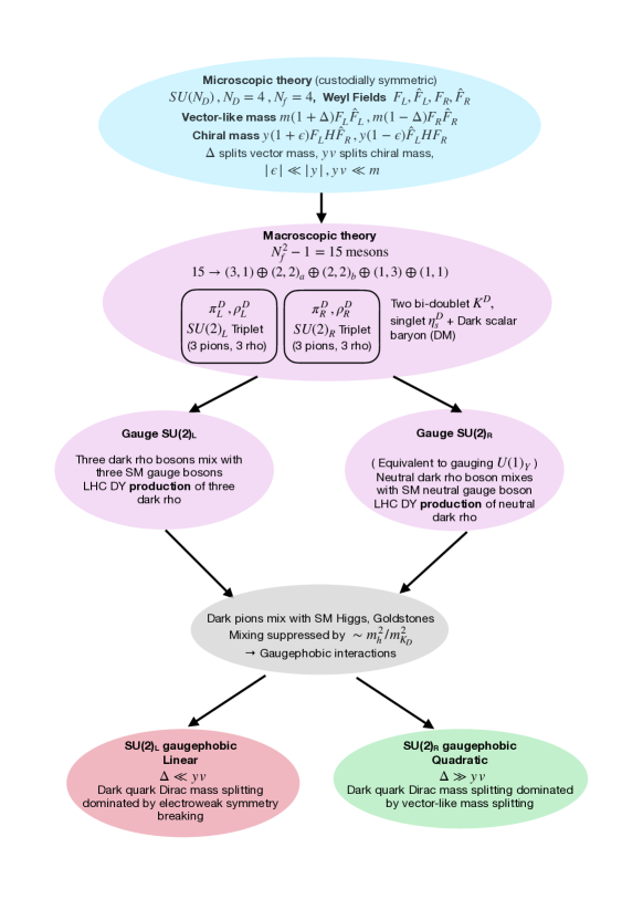
Figure 1: Flowchart of the model parameters details. Throughout this work, we will use low-energy parametrization of the theory. Fields depicted as $\pi^{D}_{L},\rho^{D}_{L},\pi^{D}_{R},\rho^{D}_{R}$ are referred to as $\pi_{D}$ and $\rho_{D}$ in the text without $L,R$ indices, since they serve no purpose other than to illustrate multiplicity.

Finally, the origin of DM phenomenology in this model deserves some discussion. The model features a scalar dark baryon which is stable by virtue of dark baryon symmetry. As the dark quark masses have contributions from electroweak symmetry breaking, it also gives rise to scalar baryon (DM) interactions with the Higgs boson, leading to a Higgs-mediated signal at direct-detection experiments. The two mass terms also imply that dark quarks, and consequently the dark baryon, have a tuneable coupling to the Higgs boson.

Due to the strongly-interacting nature of the theory, lattice computations prove to be useful for determining the inputs for the low-energy effective theory. For this model, such lattice simulations were performed for quenched masses in comparable regime scenario $\Lambda\sim m_{q_{D}}$. These simulations provide us with the spectra of $\pi_{D}$, $\rho_{D}$ and dark baryon masses for certain values of the pion to rho mass ratio ($m_{\pi_{D}}/m_{\rho_{D}}\equiv\eta$) in units of a dimensionful scaling parameter. Along with this, the calculations provide the matrix element for dark baryon scattering via Higgs at direct-detection experiments, parametrised as $f^{DM}_{f}$ for the same values of $\eta$. We use these quantities as inputs for our study. We will ultimately derive constraints the tuneable Higgs to dark quark coupling.

The above discussion is summarised as a flowchart in Figure 1. For the sake of clarity we use explicit left and right indices for $\pi_{D},\rho_{D}$ in the figure. In the discussions however, we drop these indices assuming that the dark rhos and pions belong to the representation of choice.

In practical terms, we use the effective Lagrangians as implemented in Kribs et al. (2019a). This Lagrangian does not contain dark kaon production, despite them being at a similar mass scale to the dark pion. The dark kaons are expected to be produced via their mixing with the SM Higgs bosons and will in general lead to small a production cross section, due to the mixing suppression and high masses. Thus, only phenomenology of dark pions and rhos is considered.

For the low-energy parametrization, one can write an effective Lagrangians where dark pion couplings to gauge bosons are suppressed by $\xi\sim m_{h}^{2}/m^{2}_{K_{D}}$, as discussed above, or take $\xi$ to be a free parameter and set it to 1. When $\xi=1$, the pion couplings to gauge bosons are unsuppressed and this leads to a so-called ‘gaugephilic’ scenario. For such a scenario to exist, the dark pions should be in the $SU(2)_{L}$ representation and hence (only) the low-energy parametrization of the $SU(2)_{L}$ model involves a gaugephilic scenario as well.

An example of such a gaugephilic scenario can be realised in, for example, two-flavour chiral theory, and is discussed at length in Kribs et al. (2019b). For theories containing two flavours, there is no scalar baryon hence no dark matter candidate. We will discuss gaugephilic scenarios from the point of view of their collider phenomenology; however no connection to the DM phenomenology will be made.

III Dark mesons and collider phenomenology

As discussed above, the kinematic mixing of the $\rho_{D}$ with SM gauge bosons opens the possibility of its production via quark-antiquark annihilation (DY). If kinematically allowed, the decay of the $\rho_{D}$ to $\pi_{D}$ pairs is possible. The $\rho_{D}$ may also decay directly to SM fermion-antifermion pairs. In the gaugephobic case, the $\pi_{D}$ decays primarily to pairs of fermions, while in gaugephilic cases it may also decay via $W+h$ or $Z+h$ if this is kinematically allowed.

III.1 $\rho_{D}$ and $\pi_{D}$ production and decay at the LHC

In our study we calculate the cross-section for $\rho_{D}$ and $\pi_{D}$ production using Herwig Bellm et al. (2019) to simulate events based upon the Feynrules model files Degrande et al. (2012) provided by Kribs et al Kribs et al. (2019a). We scan over various parameter planes of the model, generating all leading-order 2 $\to$ 2 processes in which at least one dark meson is either an outgoing leg, or an $s$-channel resonance.

The most important dark meson production mechanism at the LHC is single $\rho_{D}$ production, often in association with another hard particle, with the cross-sections for SU$(2)_{\textrm{L}}$ models typically an order of magnitude larger than for SU$(2)_{\textrm{R}}$ models.

Assuming 13 TeV $pp$ collisions, the largest cross-sections come from $\rho_{D}$ particles produced with a quark or gluon (for a $m_{\rho_{D}}\sim 1$ TeV, of the order of 100 fb each for $\rho_{D}^{0}$, $\rho_{D}^{+}$ and $\rho_{D}^{-}$ for SU$(2)_{\textrm{L}}$, and of the order of 10 fb, for $\rho_{D}^{0}$ only, in SU$(2)_{\textrm{R}}$). The $\rho_{D}$ can also be produced in association with a weak vector boson, with a cross-section about an order of magnitude less than for quarks and gluons in the SU$(2)_{\textrm{L}}$ case. In the SU$(2)_{\textrm{R}}$ case, production with weak bosons is negligible. Finally, the $\rho_{D}$ can be produced with a photon, with cross-sections around $1$ and $0.1$ fb for SU$(2)_{\textrm{L}}$ and SU$(2)_{\textrm{R}}$ respectively. Herwig will also generate $\pi_{D}$ pair production mediated via an $s$-channel $\rho_{D}$, taking into account the calculated $\rho_{D}$ width.

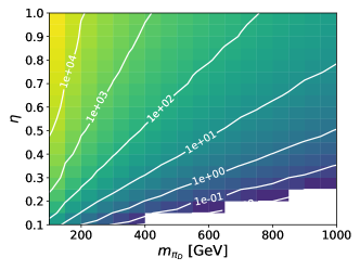
(a) $pp\rightarrow\rho_{D}^{0}q$ (SU$(2)_{\textrm{L}}$)

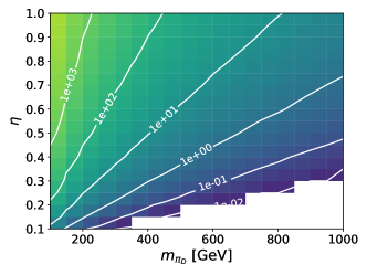
(b) $pp\rightarrow\rho_{D}^{0}q$ (SU$(2)_{\textrm{R}}$)

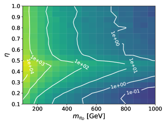
(c) $pp\rightarrow\pi_{D}^{+}\pi_{D}^{-}$ (SU$(2)_{\textrm{L}}$)

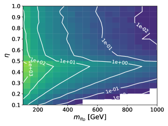
(d) $pp\rightarrow\pi_{D}^{+}\pi_{D}^{-}$ (SU$(2)_{\textrm{R}}$)

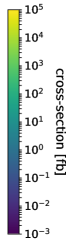
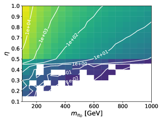
(e) $s$-channel $pp\rightarrow\rho_{D}\rightarrow l^{+}l^{-}$ (SU$(2)_{\textrm{L}}$)

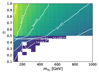
(f) $s$-channel $pp\rightarrow\rho_{D}\rightarrow l^{+}l^{-}$ (SU$(2)_{\textrm{R}}$)

Figure 2: Selected BSM cross-sections as a function of $m_{\pi_{D}}$ and $\eta$, for 13 TeV $pp$ collisions. The left (a,c,e) and right (b,d,f) columns shows cross-sections for SU$(2)_{\textrm{L}}$ and SU$(2)_{\textrm{R}}$ respectively. The shapes are qualitatively similar, but the cross-sections for the latter are about an order of magnitude smaller. The gaugephilic/gaugephobic distinction does not make a qualitative difference. Below the $\eta=0.5$ boundary, $\rho_{D}$ decays primarily to $\pi_{D}$ pairs, and this is enhanced at the threshold. Above, $\rho_{D}$ decays to pairs of fermions dominate. White areas indicate regions where the estimated cross-section is below $10^{-3}$ fb.

Once produced, the decay of a $\rho_{D}$ depends on the mass hierarchy of the dark mesons. If $\rho_{D}\rightarrow\pi_{D}\pi_{D}$ is kinematically allowed ($\eta\leq 0.5$), then this is by far the dominant decay mechanism, with over 99% branching fraction (and sub-percent level fractions of decays to fermions or quarks). On the other hand, if the $\rho_{D}$ cannot decay to $\pi_{D}$, it decays 25% of the time to each generation of quark, with the remaining branching fraction is shared equally between decays to each generation of leptons.

Pair-production of $\pi_{D}$ via a virtual $\rho_{D}$ is maximised when $m_{\rho_{D}}$ is twice $m_{\pi_{D}}$ ($\eta=0.5$), as expected. For the SU$(2)_{\textrm{L}}$ model, this process can reach about $10^{4}$ fb for $m_{\rho_{D}}\sim 1$ TeV, or $10^{3}$ fb in the SU$(2)_{\textrm{R}}$ model. Dark pions can also be singly-produced with a quark or gluon. This process is independent of the mass of the $\rho_{D}$, and is typically of the order of 1-10 fb for a pion mass of 1 TeV. Finally, $s$-channel production of pairs of leptons or quarks (and also $t$-channel for quarks) via a $\rho_{D}$ can be large, around 10 fb in the SU$(2)_{\textrm{R}}$ model and 10-100 fb for the SU$(2)_{\textrm{L}}$ model, where in addition lepton-neutrino pairs can be produced if the intermediate particle was a charged $\rho_{D}$. Examples of some of the subprocess cross-sections as a function of $\eta$ and $m_{\pi_{D}}$ for the processes mentioned above are shown in Fig. 2, for 13 TeV $pp$ collisions.

III.2 Expected experimental signatures at the LHC

Given the cross-section results, the LHC experimental signatures which are expected to be the most sensitive to these models will also depend on the mass hierarchy of the $\rho_{D}$ and $\pi_{D}$, as well as the handedness and the gaugephobic or gaugephilic nature of the model. For $\eta>0.5$, the singly-produced $\rho_{D}^{0}$ decaying to leptons can provide a clean signature that should be visible in high-mass DY measurements and searches. This is the case for all types of model considered. One may also expect a large cross-section of dijet, or $t\bar{t}$-like signatures (from $\rho_{D}$ decays to quarks), but such hadronic-only signatures would be far more difficult to distinguish from the QCD background at the LHC. For $\eta<0.5$, the expected signatures depend more on the $\pi_{D}$ decay modes: in gaugephobic models, the dominant decay of charged and neutral $\pi_{D}$ is to a mixture of third-generation quarks (once above the kinematic threshold), leading to a multijet signature, suggesting that measurements of $t\bar{t}$, and/or final states involving $b$-tagged jets, will be most sensitive. Otherwise, one would need to rely on the accompanying decay of a vector boson to select events: this means that $Z+$jets or $W$+jets signatures might be expected to give good sensitivity. On the other hand, for gaugephilic models there are regions where the dominant branching fraction for $\pi_{D}$ particles involves a vector boson and a Higgs boson, with decays to third generation quarks still important depending upon the $\pi_{D}$ mass region. In this case, $Z+$jets or $W$+jets signatures can also be expected to play a role.

IV Collider constraints on Dark Meson Production

We scan over the parameter planes of the model, and use Contur v2.1.1 to identify parameter points for which an observably significant number of events would have entered the fiducial phase space of the measurements available in Rivet 3.1.4 ,. Contur evaluates the discrepancy this would have caused, under the assumption that the measured values, which have all been shown to be consistent with the SM, are identical to it. This is used to derive an exclusion for each parameter point, taking into account correlations between experimental uncertainties where available. The ATLAS run 2 dilepton resonance search Aad et al. (2019) is also available in Rivet and is used, with some caveats since in this case the SM background is modelled by a fit to data rather than a precision calculation; the impact of this will be discussed below.

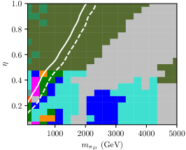
(a)

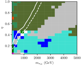
(b)

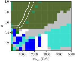
(c)

Figure 3: Scans in $\eta\--m_{\pi_{D}}$ for three sub-models. (a) Gaugephilic SU$(2)_{\textrm{L}}$, (b) Gaugephobic SU$(2)_{\textrm{L}}$ (c) Gaugephobic SU$(2)_{\textrm{R}}$. The colours indicate the dominant signature pool giving the sensitivity. The white solid line is the 95% exclusion and the white dashed line is the 68% exclusion.

CMS high-mass DY $\ell\ell$	ATLAS high-mass DY $\ell\ell$	ATLAS $\ell_{1}\ell_{2}$+$E_{T}^{\rm miss}$+jet
ATLAS $ee$+jet	ATLAS $E_{T}^{\rm miss}$+jet	ATLAS jets
ATLAS Hadronic $t\bar{t}$	ATLAS 4$\ell$	ATLAS $\ell$+$E_{T}^{\rm miss}$+jet
ATLAS $\mu\mu$+jet

Scans are performed in the $\eta\--m_{\pi_{D}}$ plane for the Gaugephilic SU$(2)_{\textrm{L}}$, Gaugephobic SU$(2)_{\textrm{L}}$ and Gaugephobic SU$(2)_{\textrm{R}}$ sub-models, and shown in Fig. 3.

The expected change in behaviour around $\eta=0.5$ is clearly seen. The dominant exclusion for much of the plane comes from the 139 fb^-1 ATLAS dilepton search, with the CMS measurement using 3.2 fb^-1 Sirunyan et al. (2019b) and the ATLAS 7 and 8 TeV measurements Aad et al. (2013, 2016) all having an impact at lower $m_{\pi_{D}}$. No dilepton measurements using the full run 2 integrated luminosity from the LHC are yet available. For the $\eta>0.5$ region, the $\rho_{D}^{0}$ decay does indeed produce a resonant signature, as may be seen for an example point in Fig.4a, and so this limit can be taken as a good estimate. In this case, $\rho_{D}$ masses as high as 2 TeV are excluded for $\eta$ close to unity in the left-handed cases, with this limit being reduced to around 1.7 TeV for the SU$(2)_{\textrm{R}}$ model due to the generally lower cross-section. Example plots leading to the exclusion are shown in Fig. 4.

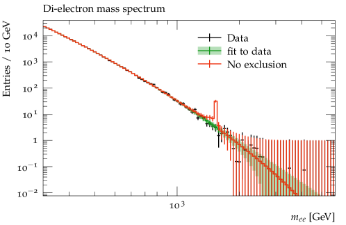
(a)

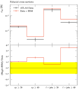
(b)

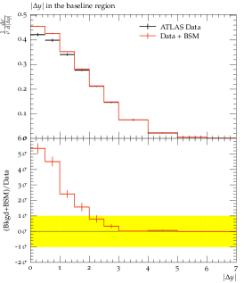
(c)

Figure 4: Example kinematic distributions for the Gaugephobic SU$(2)_{\textrm{L}}$ model. (a) Di-electron mass distribution from Aad et al. (2019), $m_{\pi_{D}}=1.4$ TeV, $\eta=0.9$. The uncertainties on the data and on the BSM are statistical only, those on the background fit include the systematics. (b) $t\bar{t}b\bar{b}$ cross-sections Aaboud et al. (2019), $m_{\pi_{D}}=390$ GeV, $\eta=0.45$. Full uncertainties are shown on the data, and by the yellow band in the lower ratio plot. (c) ATLAS dilepton+jets measurement Aad et al. (2014a), $m_{\pi_{D}}=260$ GeV, $\eta=0.4$. Uncertainties shown as in (c)

This challenging $\eta<0.5$ region requires further discussion, and in Fig. 3 exclusions from a wide variety of other final states contribute, reflecting the many possible $\pi_{D}$ decay chains. For the SU$(2)_{\textrm{L}}$ cases, there is also some apparent sensitivity in this region from the dilepton search, although it no longer domninates. However, while lepton pairs may be produced in $\pi_{D}$ decays, for example via top quarks, they are no longer resonant at the $\rho_{D}$ mass and so the “bump hunt” approach of Aad et al. (2019) is no longer valid. In this case, we revert to the default Contur mode, which uses only particle-level measurements, and re-scan the region $\eta<0.5$ at low $m_{\pi_{D}}$. This allows a more detailed investigation of the different $\pi_{D}$ decay signatures. The results are shown in Fig. 5.

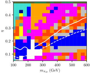
(a)

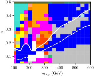
(b)

Figure 5: Scans in $\eta\--m_{\pi_{D}}$ for two sub-models, focussing on the $\eta<0.5$ region and excluding the ATLAS dilepton search. (a) Gaugephilic SU$(2)_{\textrm{L}}$, (b) Gaugephobic SU$(2)_{\textrm{L}}$ The colours indicate the dominant signature pool giving the sensitivity. The white solid line is the 95% exclusion and the white dashed line is the 68% exclusion.

CMS $ee$+jet	CMS $\mu\mu$+jet	ATLAS $ee$+jet
ATLAS $\ell\ell$+jet	ATLAS $\mu\mu$+jet	ATLAS $\ell$+$E_{T}^{\rm miss}$+jet
ATLAS $\mu$+$E_{T}^{\rm miss}$+jet	ATLAS $e$+$E_{T}^{\rm miss}$+jet	CMS $\ell$+$E_{T}^{\rm miss}$+jet
ATLAS Hadronic $t\bar{t}$	ATLAS $\ell_{1}\ell_{2}$+$E_{T}^{\rm miss}$+jet	ATLAS high-mass DY $\ell\ell$
CMS high-mass DY $\ell\ell$	ATLAS 4$\ell$	ATLAS $\gamma$
ATLAS $\ell\ell\gamma$	ATLAS $\gamma$+$E_{T}^{\rm miss}$	ATLAS jets

With finer granularity of the scan, a mix of other analyses can now be seen to be contributing to the exclusion.

• when $m_{\pi_{D}}$ falls in the Higgs mass window of the ATLAS $H\rightarrow\gamma\gamma$ fiducial cross-section measurement Aad et al. (2014b), the $\pi_{D}\rightarrow\gamma\gamma$ decays populate the cross-section and, despite their suppression due to dark flavour symmetry Kribs et al. (2019b), would have led to an observable excess at high $p_{T}^{\gamma\gamma}$, had they been present.

• for $\eta\approx 0.2$ and $m_{\pi_{D}}\approx 220$ GeV, the boosted hadronic top measurement Aaboud et al. (2018) is most sensitive; tops are produced in the dominant decay modes of both neutral and charged $\pi_{D}$ in this region, and for low $\eta$, where the $\rho_{D}$ is much heavier than the $\pi_{D}$, they will indeed be boosted.

• at low $m_{\pi_{D}}$ and $\eta$ just below 0.5, the most sensitive measurements are of $t\bar{t}$ production in the $e\mu$ channel Aad et al. (2020), where an excess at low transverse momentum of the $e\mu$ system would have been particularly prominent.

• at higher $\eta$ values, and especially in the gaugephilic case, the full run 2 four-lepton measurement Aad et al. (2021) is sensitive for $m_{\pi_{D}}\approx 200$ GeV and above. In this region $\pi_{D}\pi_{D}\rightarrow Zht\bar{b}$ is significant, and can give rise to such signatures, as can $\pi_{D}\pi_{D}\rightarrow hhZW$ and $\pi_{D}\pi_{D}\rightarrow hhWW$ (in the gaugephilic case) if kinematically possible.

• at low $m_{\pi_{D}}$ and $\eta$, and in the gaugephobic case also at higher $\eta$ and $m_{\pi_{D}}\approx 400$ GeV, lepton missing transverse energy and jet final states are important. In both cases this is due to $\pi_{D}\pi_{D}\rightarrow t\bar{t}t\bar{b}$, with the ATLAS $t\bar{t}+b$-jets measurement Aaboud et al. (2019) being especially powerful, where a significant excess in the $\ell+\geq 4b$ cross-section should have been visible, as shown in Fig. 4b.

• in the $0.3<\eta<0.5$ region for $m_{\pi_{D}}>220$ GeV, measurements of dilepton plus jetsAad et al. (2014a); Khachatryan et al. (2017) are sensitive, especially in the gaugephilic case. This is due the $\pi_{D}\pi_{D}\rightarrow Zht\bar{b}$ (in both models) and the $\pi_{D}\pi_{D}\rightarrow hhZW$ and $\pi_{D}\pi_{D}\rightarrow hhWW$ decay modes (in the gaugephilic case). An example distribution is shown in Fig. 4c.

• The high mass DY measurements Aad et al. (2016); Sirunyan et al. (2019b) also still play a role in the total exclusion, although they are rarely dominant. This indicates that future measurements should be powerful.

V Implications for Dark Matter Phenomenology

Taking the searches considered in Kribs et al. (2019a), along with the constraints derived in the previous two sections, we now consider the implications for stealth DM models. In Ref. Appelquist et al. (2015), the authors demonstrate potential ways to connect collider limits with DM analysis. We follow this strategy here in order to connect the different regimes together. It should be noted that unlike WIMP theories consisting of elementary particles, the LHC signals in our scenarios are not directly related to the production of dark matter. It is by using the underlying fundamental theory of dark quarks in the SU(4) fundamental representation, which fixes the mass spectra, that we can connect seemingly unrelated LHC signatures to DM phenomenology.

From our results of the previous section, we obtain excluded values of $\eta$ and $m_{\pi_{D}}$. These can be used to obtain the corresponding DM mass $m_{\textnormal{DM}}$ via

$$m_{S0}(\eta)=m_{B}(\eta)=m_{\textnormal{DM}}(\eta)=\frac{amS0(\eta)}{amps(\eta)}\times m_{\pi_{D}}(\eta)$$ (1)

where $amS0,amps$ are the masses predicted by lattice simulations, and $m_{\pi_{D}}$ is the excluded pseudo-scalar mass obtained in the previous section. The exact values of $amS0,amps$ are summarised in Table 1. We interpolate between different $\eta$ values in order to get Fig. 6. Finally, when $\eta\to 1$, we approach the heavy quark limit. In this limit, the masses of bound states are simply sum of the masses of the constituent quarks. In this case the scalar baryon mass, being made up of four quarks, should be twice $m_{\pi_{D}}$, which has two constituent quarks. Having observed that such a limit is already reached for $\eta=0.77$, we keep the mass ratios constant beyond for higher $\eta$ values.

$\eta$	$amps$	$amv$	$amS0$	$f^{DM}_{f}$
0.77	0.3477	0.4549	0.9828	0.153
0.70	0.2886	0.4170	0.8831	0.262
0.50	0.2066	0.3783	0.7687	0.338

Table 1: Lattice inputs for $\beta=11.028$ on $32^{3}\times 64$ lattices taken from Appelquist et al. (2014) for this work. $amps,amv$ and $amS0$ represent dimensionless pseudo-scalar, vector and dark baryon masses while $f^{(DM)}_{f}$ is lattice input for computing DM direct-detection cross-section via Higgs exchange.

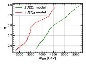
Figure 6: Limits on the mass of dark matter given constraints on $m_{\pi_{D}}$ and $m_{\rho_{D}}$ for the SU$(2)_{\textrm{L}}$ model (green) and the SU$(2)_{\textrm{R}}$ model (red). As discussed in the text, only gaugephobic limits are used. The solid lines represent the region where lattice results are available, whilst the dashed lines represent our extrapolation assuming the heavy quark limit has been achieved.

The results are illustrated in Fig. 6, where we demonstrate exclusion limits on $m_{\textnormal{DM}}$ as a function of $\eta$. The two curves correspond to SU$(2)_{\textrm{L}}$ (green) and SU$(2)_{\textrm{R}}$ (red) gaugephobic models respectively. The dashed lines represent our extension of the provided lattice results to the heavy quark limits. We can see that the two limits differ significantly for smaller $m_{\textnormal{DM}}$, where limits on $\eta$ in the SU$(2)_{\textrm{L}}$ theory are very different to those from SU$(2)_{\textrm{R}}$ theory, as discussed in the previous section. For higher $m_{\textnormal{DM}}$ the two scenarios lead to more similar limits on $\eta$, pushing the allowed $m_{\textnormal{DM}}$ to the multi-TeV regime. The limits from SU$(2)_{\textrm{R}}$ scenarios are always somewhat weaker than corresponding limits in SU$(2)_{\textrm{L}}$ theories.

VI Combined Constraints

As discussed previously, the DM candidate couples to the SM Higgs and scatters off nuclei at direct-detection experiments. The dark matter-nucleus scattering element constitutes of two parts, one corresponding to matrix element of the fermions in the scalar baryons ($f_{f}^{DM}$) which is computed via lattice simulation Appelquist et al. (2014) and second, the Yukawa coupling between Higgs and dark quarks. Unfortunately, the Yukawa coupling as defined in Section II and also introduced in Fig. 1 can not be directly constrained and hence needs to be recast into so-called $y_{\textrm{eff}}$ parameter which is independent of dark fermion mass Appelquist et al. (2015). We identify that the so-called linear case as discussed in Appelquist et al. (2015) corresponds to the gaugephobic SU$(2)_{\textrm{L}}$ case, while the quadratic case corresponds to the SU$(2)_{\textrm{R}}$ gaugephobic case. This can be understood as follows. As explained in Section II, the dark quarks obtain their masses from the vector as well as electroweak symmetry breaking (EWSB) mass terms. The physical masses are thus a mixture of the two mass terms after mass diagonalization. The coupling of Higgs to these physical quark masses will be proportional to the Higgs–dark quark Yukawa coupling times the mass of the dark quark, just like in the SM. If the dark quark masses are dominated by EWBS (chiral) mass term, one gets a quadratic dependence of Higgs–dark quark coupling, otherwise a linear dependence. Therefore, in the linear (SU$(2)_{\textrm{L}}$) case, EWSB is dominantly (but not entirely) responsible for quark mass splitting, while the situation reverses in the other limit. It should be noted that $y_{\textrm{eff}}$ is a free parameter of the theory and can be constrained using experimental data which is exactly what we will do in this section by combining latest Xenon1T limits with the LHC limits and obtain maximum allowed coupling $y_{\textrm{eff}}$ between the dark quarks and Higgs. We briefly outline the exact procedure we follow in order to compute the DM–nucleus scattering cross-sections which closely followsAppelquist et al. (2014, 2015).

The dark matter nucleus spin-independent scattering cross-section is given by

$$\sigma(\textrm{DM},N)=\displaystyle\frac{\mu(m_{\textrm{DM}},m_{N})^{2}}{\pi}\left(Z\mathcal{M}_{p}+(A-Z)\mathcal{M}_{n}\right)^{2},$$ (2)

where $N$ is the nucleus, $\mu(m_{\textrm{DM}},m_{N})$ represents the nucleus - dark matter reduced mass, Z, A are the atomic and mass numbers, here taken for Xenon and finally $\mathcal{M}_{p,n}$ are the amplitudes for scattering off proton or neutron. This quantity is dependent on the experiment target, in order to ease the comparison among different experiments the cross-section is conveniently expressed as

$$\sigma_{0}(\textrm{DM},a)=\sigma(\textrm{DM},N)\displaystyle\frac{\mu(m_{\textrm{DM}},m_{a})^{2}}{\mu(m_{\textrm{DM}},m_{N})^{2}\,A^{2}},$$ (3)

where $\sigma_{0}(\textrm{DM},a)$ is the scattering cross-section per nucleon at zero momentum transfer. The DM–nucleus scattering cross-section mediated by the Higgs exchange contains two parts, the first corresponding to the Higgs–SM quark current while the other contains Higgs–DM exchange.

In particular the amplitude is given by

$$\mathcal{M}_{p,n}=\frac{g_{p,n}\,g_{DM}}{m_{h}^{2}}$$ (4)

with

$$g_{p,n}=\frac{m_{p,n}}{v}\left[\sum_{q=u,d,s}f_{q}^{(p,n)}+\frac{6}{27}\left(1-\sum_{q=u,d,s}f_{q}^{(p,n)}\right)\right]\\$$ (5)

and

$$g_{DM}\simeq\begin{cases}y_{\textrm{eff}}\,f_{f}^{DM},&\text{{SU}$(2)_{\textrm{L}}$ case}\\ \\ y_{\textrm{eff}}^{2}\,\displaystyle\frac{v}{m_{\textnormal{DM}}}f_{f}^{DM},&\text{{SU}$(2)_{\textrm{R}}$ case}\end{cases}$$ (6)

The quantity $f_{f}^{DM}$ is extracted from lattice calculations and precise values are tabulated in Table 1, while $y_{\textrm{eff}}$ is the effective Yukawa coupling independent of the dark quark masses. Using the definitions above and the lattice parameters for $f_{q}^{(p,n)}$ as defined in Hill and Solon (2012); Belanger et al. (2009), we update the constraints on $y_{\textrm{eff}}$, as shown in Fig.7 and Fig.8.

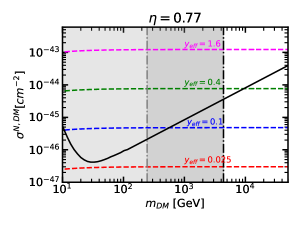
(a)

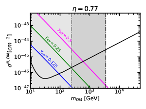
(b)

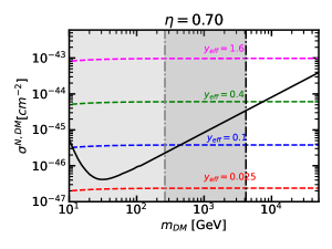
(c)

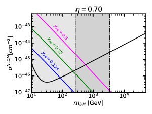
(d)

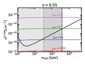
(e)

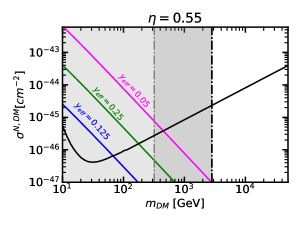
(f)

Figure 7: Left panels (a,c,e), constraints for SU$(2)_{\textrm{R}}$ model and right panels (b,d,f), constraints $SU(2)_{L}$ model, for several values of $\eta$. Colored contours show DM–SM scattering cross-sections for fixed value of $y_{\textrm{eff}}$, vertical lines represent $m_{\textnormal{DM}}$ limits derived from LEP limits on pion mass (grey dot-dashed line) and updated LHC constraints derived in this work (black dot-dashed line). Also overlaid are the recent Xenon1T constraints on DM–nucleon coherent scattering. Aprile et al. (2018).

To begin with, in Fig.7, we show contours of $y_{\textrm{eff}}$ in the $m_{\textnormal{DM}}$ and DM–nucleon scattering cross-section plane for SU$(2)_{\textrm{R}}$ model (left panels) and SU$(2)_{\textrm{L}}$ case (right panels) for fixed value of $\eta$ of 0.77 (a,b), 0.70 (c,d) and 0.55 (e,f). The values of $\eta$ correspond to those for which lattice calculations are performed. We also overlay the latest Xenon1T DM–nucleon elastic scattering cross-section limits Aprile et al. (2018). The way to interpret this plot would be to find values of $y_{\textrm{eff}}$ which lie below the Xenon1T curve for a given $m_{\textnormal{DM}}$. These correspond to direct detection allowed parameter spaces. Finally, we also show illustrate exclusions on $m_{\textnormal{DM}}$ obtained from LEP II limits  in Kribs et al. (2019b) (dot-dashed grey line) and from our LHC analysis as discussed in section above (dot-dashed black line). Combining this with the DM–nucleon scattering cross-section limits, one can then derive the maximum value of $y_{\textrm{eff}}$ which obeys all limits. Stringent limits on $y_{\textrm{eff}}$ imply weaker coupling between DM and Higgs and thus in general weaker DM–SM interactions.

Before discussing the ultimate lessons we learn from this, we first discuss Fig.7. As expected from Eq.6, for the SU$(2)_{\textrm{R}}$ case the DM–nucleon scattering cross-section is independent of $m_{\textnormal{DM}}$ while for SU$(2)_{\textrm{L}}$ case it is inversely proportional to $m_{\textnormal{DM}}$ for a given value of $y_{\textrm{eff}}$. For SU$(2)_{\textrm{R}}$ case, the Xenon1T allowed value of $y_{\textrm{eff}}$ decreases as $\eta$ increases, this is because $f^{DM}_{f}$ increases as $\eta$ increases. The dependence is more complicated for SU$(2)_{\textrm{L}}$ case where $g_{DM}$ depends on both $f^{DM}_{f}$ and $m_{\textnormal{DM}}$ which increase as $\eta$ increases. However $f^{DM}_{f}$ increases faster than $m_{\textnormal{DM}}$ and hence $y_{\textrm{eff}}$ decreases albeit at a smaller rate.

Finally, the limits from DM–nucleon elastic scattering are complemented by the limits on $m_{\textnormal{DM}}$ derived by LEP and LHC analyses. In particular, for each $\eta$, the corresponding figure illustrates the impact of updated LHC limits compared to the LEP exclusion. The LHC limits as obtained by us in this analysis together with the Xenon1T limits thus either demand smaller values of $y_{\textrm{eff}}$ or large $m_{\textnormal{DM}}$ to be compatible with current experimental situation. This is precisely reflected in Fig. 8, where we plot the maximum allowed values of $y_{\textrm{eff}}$ for various value of $\eta$ (solid lines) and overlay the limits obtained from LHC (dot-dashed line). It should be noted that lower values of $\eta$ push the theory into the chiral (massless quark) limit where no lattice results are available, and we refrain from deriving any limits in this region.

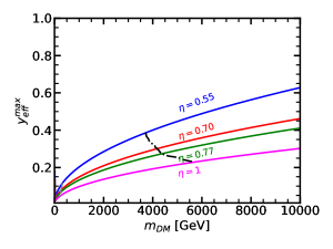
(a)

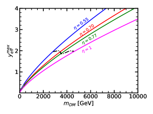
(b)

Figure 8: (a) Maximum allowed value of $y_{\textrm{eff}}$ for given value of $\eta$ for SU$(2)_{\textrm{L}}$ model, (b) constraints SU$(2)_{\textrm{R}}$ model. The black dot dashed line shows LHC limits derived in this work. Unlike Applequist et alAppelquist et al. (2015), we do not extend our LHC limits in the chiral limit (ie low $\eta$), meaning we have an abrupt cut-off in the LHC limits around $m_{\textnormal{DM}}$ of about 3.5 TeV (a) and 3 TeV (b) respectively.

VII Relic Density Implications

Global investigations, first carried out in Ref. Kribs et al. (2019b); Appelquist et al. (2015); Kribs et al. (2019a) and this analysis, can have implications for possible relic density generation mechanisms in the underlying composite SU(4) theories. As argued in Ref. Appelquist et al. (2015), there are two broad avenues to obtain relic density. The first is so-called symmetric abundance mechanism, where annihilation of dark baryons into dark mesons controls the relic density in a way akin to the WIMP mechanism. Being entirely within the dark sector, this annihilation channel is expected to dominate. From simple dimensional analysis, one expects baryon masses to be $\sim 100\,\rm{TeV}$ for relic abundance to be satisfied. However, a precise calculation of this requires knowledge of annihilation channels. Within the framework of chiral perturbation theory, this means one needs to include baryons, which is non-trivial. The other way is to perform lattice simulations of scattering amplitudes, which are absent for the model we work with.

The other possibility is to obtain relic abundance from the decays of the electroweak sphaleron – the non-perturbative solution at finite temperature that allows transition between different vacua with different $B+L$ numbers. This corresponds to the so-called asymmetric mechanism. Given that dark fermions are charged under the SM gauge group, the electroweak sphalerons also contribute to generation of dark baryons during the decay after sphaleron “freeze-out”. Whether such decays generate any asymmetry, which further affects dark baryon number generation is also an important consideration. In cases where there is no asymmetry, previous calculations for techibaryon models Nussinov (1985); Chivukula and Walker (1990); Barr et al. (1990) have shown viable dark baryon masses in 1-2 TeV ranges. However these technibaryon models rely on dark fermion mass generation purely from the EWSB mechanism. In this work, as the dark fermion masses are a combination of vector confinement and the EWSB mechanism, one can qualitatively understand the relic density generation mechanisms, but quantitative estimates are harder. If there is an initial asymmetry, e.g. in a globally conserved quantity, one could also obtain the correct abundance.

Given the model dependence of these calculations, and absence of lattice results, we refrain from making further statements about dark baryon relic density. However, we note that the LHC limits presented here and in Ref. Kribs et al. (2019b); Appelquist et al. (2015); Kribs et al. (2019a) can be relevant for scenarios in which the DM relic density is generated via sphaleron processes. Finally, we also note that relic density generation via symmetric mechanisms (i.e. when annihilation proceeds within dark sectors) will still be a viable avenue.

VIII Conclusions

The analysis presented in this paper is significant in two respects. First, we take into account the updated Xenon1T limits which are almost an order of magnitude stronger than the previous iteration. Second, the updated LHC limits (now including those from measurements as well as searches) push $m_{\textnormal{DM}}$ to the multi-TeV regime, and much stronger than any previously obtained.

When the $\rho_{D}$ decays directly to SM particles, these limits probe some scenarios in which the DM relic density is generated via sphaleron processes. However, the LHC limits as derived in Kribs et al. (2019a) and in this work are relatively weak for small $\eta$, where $\rho_{D}\to\pi_{D}\pi_{D}$ decays are open. Small values of $\eta$ also correspond to the chiral limit of the theory. Therefore we conclude that on the theory side, more efforts are needed to constrain chiral limit of such strongly-interacting scenarios. From the experimental point of view, limits on this region can be expected to improve as more precise measurements of a variety of final states are made, including tops, $b$-quarks and dileptons. As pointed out in Kribs et al. (2019a), for $m_{\pi_{D}}<150$ GeV or so, final states involving $\tau$ leptons are important. No such measurements are currently available; should they be made in future, they could have significant impact.

Overall, while some the general properties of these models can be surmised, the detailed phenomenology has many uncertainties, in particular driven by the unknown strong dynamics. This makes dedicated search analyses for specific benchmark scenarios of limited interest. While scenarios (as mentioned in the introduction) which lead to non-SM like final states will still require dedicated search strategies, the uncertainty in the phenomenology strongly motivates model-independent measurements of a wide variety of SM-like final states. These measurements can be then be analysed for discrepancies and, in their absence, rapidly interpretated as limits over a very broad range of parameters.

Appendix A Collider exclusions for the $N_{D}=2$ case

All the results presented in the main body of the text assumed that $N_{D}$ parameter of the models under consideration was set to $4$. However, the sensitivity of LHC constraints vary considerably with this $N_{D}$ parameter. To illustrate this effect, in this section we consider the $N_{D}=2$ case. The phenomenology and dominant production and decay modes in the $N_{D}=2$ and $N_{D}=4$ cases are broadly comparable, but the overall cross-sections are reduced by a factor of approximately 2. Analogously to the study presented in Section IV, the $m_{\pi_{D}}$ vs $\eta$ parameter planes of the Gaugephilic SU$(2)_{\textrm{L}}$, Gaugephobic SU$(2)_{\textrm{L}}$ Gaugephobic SU$(2)_{\textrm{R}}$ we scanned using Contur, but this time choosing $N_{D}=2$. The results are shown in Fig. 9.

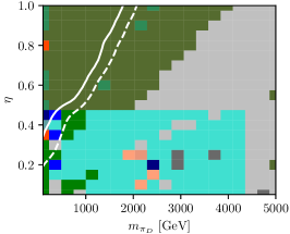
(a)

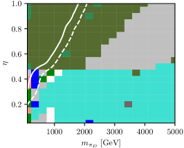
(b)

(c)

Figure 9: Scans in $\eta\--m_{\pi_{D}}$ for three sub-models. (a) Gaugephilic SU$(2)_{\textrm{L}}$, (b) Gaugephobic SU$(2)_{\textrm{L}}$ (c) Gaugephobic SU$(2)_{\textrm{R}}$. The colours indicate the dominant signature pool giving the sensitivity. The white solid line is the 95% exclusion and the white dashed line is the 68% exclusion.

ATLAS $\ell$+$E_{T}^{\rm miss}$+jet	ATLAS $e$+$E_{T}^{\rm miss}$+jet	ATLAS $\ell_{1}\ell_{2}$+$E_{T}^{\rm miss}$
ATLAS $\gamma$+$E_{T}^{\rm miss}$	ATLAS high-mass DY $\ell\ell$	ATLAS $\mu\mu$+jet
CMS $e$+$E_{T}^{\rm miss}$+jet	ATLAS $\mu$+$E_{T}^{\rm miss}$+jet	ATLAS $E_{T}^{\rm miss}$+jet
ATLAS 4$\ell$	ATLAS $ee$+jet	CMS high-mass DY $\ell\ell$
ATLAS jets	ATLAS Hadronic $t\bar{t}$	ATLAS $\ell_{1}\ell_{2}$+$E_{T}^{\rm miss}$+jet

The resulting constraints have a similar structure to the $N_{D}=4$ case (which were shown in Fig. 3). In particular, for the left-handed models, the constraints cut across the $m_{\pi_{D}}$ vs $\eta$ plane, while for the right-handed model, the sensitivity ends roughly below $\eta\sim 0.5$, as is expected.

In this case, the dominant exclusion for much of the plane still comes from the 139 fb^-1 ATLAS dilepton search, with the CMS measurement using 3.2 fb^-1 Sirunyan et al. (2019b) and the ATLAS 7 and 8 TeV measurements Aad et al. (2013, 2016) having an impact at lower $m_{\pi_{D}}$ (although less so than in the $N_{D}=4$ case).

However, the constraints are overall weaker than in the $N_{D}=4$ case, retreating in general by about $250$ GeV in $m_{\pi_{D}}$. In the SU$(2)_{\textrm{R}}$ plane, the $N_{D}=2$ results also do not reach into the $\eta<0.5$ region as they did for $N_{D}=4$.

In summary, scanning the SU$(2)_{\textrm{L}}$ and SU$(2)_{\textrm{R}}$ models where the $N_{D}$ parameter is set to $2$ instead of $4$ leads to a very similar set of results, but weaker due to an overall lower cross-section for the key processes expected at the LHC. This illustrates that the results of the study presented in this paper are sensitive to choices in parameters such as $N_{D}$, and this should be kept in mind when interpreting these results.

References

- Hochberg et al. (2014) Y. Hochberg, E. Kuflik, T. Volansky, and J. G. Wacker, Phys. Rev. Lett. 113, 171301 (2014), eprint 1402.5143.
- Tsai et al. (2020) Y.-D. Tsai, R. McGehee, and H. Murayama (2020), eprint 2008.08608.
- Lee and Seo (2015) H. M. Lee and M.-S. Seo, Phys. Lett. B 748, 316 (2015), eprint 1504.00745.
- Choi and Lee (2016) S.-M. Choi and H. M. Lee, Phys. Lett. B 758, 47 (2016), eprint 1601.03566.
- Cline et al. (2014) J. M. Cline, Z. Liu, G. Moore, and W. Xue, Phys. Rev. D 90, 015023 (2014), eprint 1312.3325.
- Boddy et al. (2014a) K. K. Boddy, J. L. Feng, M. Kaplinghat, and T. M. P. Tait, Phys. Rev. D 89, 115017 (2014a), eprint 1402.3629.
- Boddy et al. (2014b) K. K. Boddy, J. L. Feng, M. Kaplinghat, Y. Shadmi, and T. M. P. Tait, Phys. Rev. D 90, 095016 (2014b), eprint 1408.6532.
- Soni and Zhang (2016) A. Soni and Y. Zhang, Phys. Rev. D 93, 115025 (2016), eprint 1602.00714.
- Beauchesne et al. (2019) H. Beauchesne, E. Bertuzzo, and G. Grilli Di Cortona, JHEP 04, 118 (2019), eprint 1809.10152.
- Hochberg et al. (2018) Y. Hochberg, E. Kuflik, R. Mcgehee, H. Murayama, and K. Schutz, Phys. Rev. D 98, 115031 (2018), eprint 1806.10139.
- Bernreuther et al. (2020) E. Bernreuther, F. Kahlhoefer, M. Krämer, and P. Tunney, JHEP 01, 162 (2020), eprint 1907.04346.
- Mies et al. (2021) H. Mies, C. Scherb, and P. Schwaller, JHEP 04, 049 (2021), eprint 2011.13990.
- Renner and Schwaller (2018) S. Renner and P. Schwaller, JHEP 08, 052 (2018), eprint 1803.08080.
- Buckley and Neil (2013) M. R. Buckley and E. T. Neil, Phys. Rev. D 87, 043510 (2013), eprint 1209.6054.
- Appelquist et al. (2015) T. Appelquist et al., Phys. Rev. D 92, 075030 (2015), eprint 1503.04203.
- Bai and Hill (2010) Y. Bai and R. J. Hill, Phys. Rev. D 82, 111701 (2010), eprint 1005.0008.
- Kribs et al. (2010) G. D. Kribs, T. S. Roy, J. Terning, and K. M. Zurek, Phys. Rev. D 81, 095001 (2010), eprint 0909.2034.
- Appelquist et al. (2013) T. Appelquist et al. (Lattice Strong Dynamics (LSD)), Phys. Rev. D 88, 014502 (2013), eprint 1301.1693.
- Nussinov (1985) S. Nussinov, Phys. Lett. B 165, 55 (1985).
- Chivukula and Walker (1990) R. S. Chivukula and T. P. Walker, Nuclear Physics B 329, 445 (1990).
- Barr et al. (1990) S. M. Barr, R. S. Chivukula, and E. Farhi, Phys. Lett. B 241, 387 (1990).
- Ryttov and Sannino (2008) T. A. Ryttov and F. Sannino, Phys. Rev. D 78, 115010 (2008), eprint 0809.0713.
- Lewis et al. (2012) R. Lewis, C. Pica, and F. Sannino, Phys. Rev. D 85, 014504 (2012), eprint 1109.3513.
- Cacciapaglia et al. (2020) G. Cacciapaglia, C. Pica, and F. Sannino, Phys. Rept. 877, 1 (2020), eprint 2002.04914.
- Kribs and Neil (2016) G. D. Kribs and E. T. Neil, Int. J. Mod. Phys. A 31, 1643004 (2016), eprint 1604.04627.
- Cohen et al. (2015) T. Cohen, M. Lisanti, and H. K. Lou, Phys. Rev. Lett. 115, 171804 (2015), eprint 1503.00009.
- Daci et al. (2015) N. Daci, I. De Bruyn, S. Lowette, M. H. G. Tytgat, and B. Zaldivar, JHEP 11, 108 (2015), eprint 1503.05505.
- Schwaller et al. (2015) P. Schwaller, D. Stolarski, and A. Weiler, JHEP 05, 059 (2015), eprint 1502.05409.
- Kribs et al. (2019a) G. D. Kribs, A. Martin, B. Ostdiek, and T. Tong, JHEP 07, 133 (2019a), eprint 1809.10184.
- Hochberg et al. (2016) Y. Hochberg, E. Kuflik, and H. Murayama, JHEP 05, 090 (2016), eprint 1512.07917.
- Knapen et al. (2017) S. Knapen, S. Pagan Griso, M. Papucci, and D. J. Robinson, JHEP 08, 076 (2017), eprint 1612.00850.
- Harnik and Wizansky (2009) R. Harnik and T. Wizansky, Phys. Rev. D 80, 075015 (2009), eprint 0810.3948.
- Sirunyan et al. (2019a) A. M. Sirunyan et al. (CMS), JHEP 02, 179 (2019a), eprint 1810.10069.
- CMS (2020) (2020).
- Kribs et al. (2019b) G. D. Kribs, A. Martin, and T. Tong, JHEP 08, 020 (2019b), eprint 1809.10183.
- Butterworth et al. (2017) J. M. Butterworth, D. Grellscheid, M. Krämer, B. Sarrazin, and D. Yallup, JHEP 03, 078 (2017), eprint 1606.05296.
- Buckley et al. (2021) A. Buckley et al. (2021), eprint 2102.04377.
- Appelquist et al. (2014) T. Appelquist et al. (Lattice Strong Dynamics (LSD)), Phys. Rev. D 89, 094508 (2014), eprint 1402.6656.
- Bierlich et al. (2020) C. Bierlich et al., SciPost Phys. 8, 026 (2020), eprint 1912.05451.
- Read (2002) A. L. Read, J. Phys. G28, 2693 (2002), [,11(2002)].
- Buckley et al. (2020) A. Buckley, J. M. Butterworth, L. Corpe, D. Huang, and P. Sun, SciPost Phys. 9, 069 (2020), eprint 2006.07172.
- Butterworth et al. (2021) J. M. Butterworth, M. Habedank, P. Pani, and A. Vaitkus, SciPost Phys. Core 4, 003 (2021), eprint 2009.02220.
- Bellm et al. (2019) J. Bellm et al. (2019), eprint 1912.06509.
- Degrande et al. (2012) C. Degrande, C. Duhr, B. Fuks, D. Grellscheid, O. Mattelaer, and T. Reiter, Comput. Phys. Commun. 183, 1201 (2012), eprint 1108.2040.
- Aad et al. (2019) G. Aad et al. (ATLAS), Phys. Lett. B 796, 68 (2019), eprint 1903.06248.
- Sirunyan et al. (2019b) A. M. Sirunyan et al. (CMS), JHEP 12, 059 (2019b), eprint 1812.10529.
- Aad et al. (2013) G. Aad et al. (ATLAS), Phys. Lett. B 725, 223 (2013), eprint 1305.4192.
- Aad et al. (2016) G. Aad et al. (ATLAS), JHEP 08, 009 (2016), eprint 1606.01736.
- Aaboud et al. (2019) M. Aaboud et al. (ATLAS), JHEP 04, 046 (2019), eprint 1811.12113.
- Aad et al. (2014a) G. Aad et al. (ATLAS), JHEP 04, 031 (2014a), eprint 1401.7610.
- Aad et al. (2014b) G. Aad et al. (ATLAS), JHEP 09, 112 (2014b), eprint 1407.4222.
- Aaboud et al. (2018) M. Aaboud et al. (ATLAS), Phys. Rev. D 98, 012003 (2018), eprint 1801.02052.
- Aad et al. (2020) G. Aad et al. (ATLAS), Eur. Phys. J. C 80, 528 (2020), eprint 1910.08819.
- Aad et al. (2021) G. Aad et al. (ATLAS) (2021), eprint 2103.01918.
- Khachatryan et al. (2017) V. Khachatryan et al. (CMS), Eur. Phys. J. C 77, 751 (2017), eprint 1611.06507.
- Hill and Solon (2012) R. J. Hill and M. P. Solon, Phys. Lett. B 707, 539 (2012), eprint 1111.0016.
- Belanger et al. (2009) G. Belanger, F. Boudjema, A. Pukhov, and A. Semenov, Comput. Phys. Commun. 180, 747 (2009), eprint 0803.2360.
- Aprile et al. (2018) E. Aprile et al. (XENON), Phys. Rev. Lett. 121, 111302 (2018), eprint 1805.12562.
- Chivukula and Walker (1990) R. S. Chivukula and T. P. Walker, Nucl. Phys. B 329, 445 (1990).
- Egana-Ugrinovic et al. (2018) D. Egana-Ugrinovic, M. Low, and J. T. Ruderman, JHEP 05, 012 (2018), eprint 1801.05432.