Fast Game Content Adaptation Through Bayesian-based Player Modelling

Abstract

In games, as well as many user-facing systems, adapting content to users’ preferences and experience is an important challenge. This paper explores a novel method to realize this goal in the context of dynamic difficulty adjustment (DDA). Here the aim is to constantly adapt the content of a game to the skill level of the player, keeping them engaged by avoiding states that are either too difficult or too easy. Current systems for DDA rely on expensive data mining, or on hand-crafted rules designed for particular domains, and usually adapts to keep players in the flow, leaving no room for the designer to present content that is purposefully easy or difficult. This paper presents Fast Bayesian Content Adaption (FBCA), a system for DDA that is agnostic to the domain and that can target particular difficulties. We deploy this framework in two different domains: the puzzle game Sudoku, and a simple Roguelike game. By modifying the acquisition function’s optimization, we are reliably able to present a content with a bespoke difficulty for players with different skill levels in less than five iterations for Sudoku and fifteen iterations for the simple Roguelike. Our method significantly outperforms simpler DDA heuristics with the added benefit of maintaining a model of the user. These results point towards a promising alternative for content adaption in a variety of different domains.

I Introduction

The problem of creating interactive media that adapts to the user has several applications, ranging from increasing the engagement of visitors of web applications to creating tailored experiences for students in academic settings [1]. One of these applications is Dynamic Difficulty Adjustment (DDA) [2], which consists of adapting the contents of a video game to match the skill level of the player. If the game presents tasks that are too difficult or too easy, it might risk losing the player due to frustration or boredom.

Current approaches to DDA focus on specific domains (e.g. MOBAs [3], Role-Playing games [4] or fighting games [5]), and use agents and techniques that either do not generalize (such as planning agents requiring forward models [6]), or rely on an expensive process of gathering data from players before the optimization can take place [7, 8]. Also relevant is the fact that most of these approaches focus on maximized engagement and achieving flow states. However, sometimes the designer’s intent might be to purposefully present content that is difficult (i.e.  out-of-flow) for a particular player [9].

Bayesian Optimization has been recently proposed as a promising approach to DDA, since it does not rely on previously gathered information on either user or domain, and can be deployed online with only minimal specifications about the game in question [10]. However, so far this approach has only been tested with AI agents and in a single domain, while only allowing for one possible difficulty target.

We propose a new Bayesian-based method for Fast Bayesian Content Adaption and test it on DDA with human players. The method maintains a simple model of the player and leverages it for optimizing content towards a target difficulty on-the-fly in a domain-agnostic fashion. Fig. LABEL:fig:banner illustrates how the proposed approach works: (1) Players are presented with levels that are predicted to have the right difficulty by the underlying probabilistic model; (2) the model is updated once new data about the player’s performance arrives; (3) steps 1–2 are repeated until a level with the desired target difficulty is found.

We test this novel approach on two domains: the puzzle game Sudoku, and levels for a simple Roguelike game. Our results show that Bayesian Optimization is a promising alternative for domain-agnostic automatic difficulty adjustment.

II Methods and Related Work

II-A Related Work on Difficulty Adjustment

Dynamic Difficulty Adjustment (DDA) consists of adapting the difficulty of a game to the skill level of the player, trying to keep a flow state (i.e. a psychological state in which users solve tasks that match their ability). DDA algorithms work by predicting and intervening [11]. They model a so-called challenge function that stands as a proxy for difficulty (e.g. win rate, health lost, hits received, completion time) and intervene the game so as to match a particular target for this challenge function [12].

Hunicke [13] points out that DDA can help players to retain a “sense of agency and accomplishment”, presenting a system called Hamlet that leveraged inventory theory to present content to players in Half-Life [2, 13]. Since then, several other approaches and methods have been presented and studied in this context, including alternating between different-performing AI agents in MOBA games [3], player modelling via data gathering or meta-learning techniques [7, 8], and artificially restricting NPCs that are implemented as planning agents such as MCTS [6, 5]. Other DDA methods model the player using probabilities such as the the probabilities that a player would re-try, churn, or win a particular level in a mobile game [11]; the resulting probabilistic graph is then used to maximize engagement.

Dynamic Difficulty Adjustment is a particular instance of the larger field of automatic content creation and adaption. Examples in this area include work on evolving and evaluating racetracks for different player models [14]. In another example, Shaker et al. optimize the game design features of platformer games towards fun levels, where fun is defined using player models trained on questionnaires [15]. Similar efforts have been made in the Experience Management community (with the goal of creating interactive storytelling games) [16].

These approaches, however, either rely on gathering data beforehand and leveraging it to create a player model that is then used for optimization, or are domain-specific (e.g. storytellers or platformers). Bayesian Optimization serves as an alternative that is data efficient and flexible. Moreover, in contrast to AI-based approaches (like adjusting NPCs performance), Bayesian Optimization of game parameters does not rely on forward models.

Bayesian Optimization has been used a tool for automatic playtesting and DDA. Zook et al. use Active Learning to fine-tune low level parameters based on human playtests [17]. Khajah et al. [18] apply Bayesian Optimization to find game parameters in Flappy Bird and Spring Ninja (e.g. distance between pipes and gap size) that would maximize engagement, measured as volunteered time. Our work differs in the fact that we build a model of player performance, instead of player engagement. With our system, designers have the affordance to target content that is difficult for a given player in a bespoke fashion.

To the best of our knowledge, our contribution is the first example of a Bayesian Optimization-based system that models levels of difficulty for particular players, and dynamically presents bespoke content according to this model.

II-B Bayesian Optimization (B.O.) using Gaussian Process Regression

Bayesian Optimization is frequently used for optimization problems in which the objective function has no closed form, and can only be measured by expensive and noisy queries (e.g. optimizing hyperparameters in Machine Learning algorithms [19], active learning [20], finding compensatory behaviors in damaged robots [21]). The problem we tackle in this paper is indeed black-box: we have no closed analytical form for the time it would take for a player to solve a given level, having them play a level is expensive time-wise, and a player’s performance on a single level may vary if we serve it repeatedly.

There are two main components in B.O. schemes [22]: a surrogate probabilistic model that approximates the objective function, and an acquisition function that uses this probabilistic information to inform where to query next in order to maximize said objective function. A common selection for the underlying probabilistic model are Gaussian Processes [23], and two frequently used acquisition functions are Expected Improvement (EI) and the Upper Confidence Bound (UCB).

II-B1 Gaussian Process Regression

Practically speaking, a Gaussian process GP defines a Normal distribution for every point-wise approximation of a function $t(x)$ using a prior $\mu_{0}(x)$ and a kernel function $k(x,x^{\prime})$ (which governs the covariance matrix).

If we assume that the observations of the function for a set of points $\bm{x}=[x_{i}]_{i=1}^{n}$, denoted by $\bm{t}=[t(x_{i})]_{i=1}^{n}=[t_{i}]_{i=1}^{n}$, are normally distributed with mean $\bm{\mu}_{0}=[\mu_{0}(x_{i})]_{i=1}^{n}$ and covariance matrix $K=[k(x_{i},x_{j})]_{i,j=1}^{n}$, we can approximate $t(x)$ at a new point $x^{*}$ by leveraging the fact that the Gaussian distributions are closed under marginalization [23]:

$$t^{*}\,|\,x^{*},\bm{x},\bm{t}\sim\mathcal{N}( \bm{\mu}_{0}+\bm{k}_{*}^{T}(K+\sigma_{\text{noise}})^{-1}\bm{t},$$ (1)

$$k(x^{*},x^{*})-\bm{k}_{*}^{T}(K+\sigma_{\text{noise}})^{-1}\bm{k}_{*}),$$

where $\bm{k}_{*}=[k(x_{i},x^{*})]_{i=1}^{n}$ and $\sigma_{\text{noise}}\in\mathbb{R}^{+}$ is a hyperparameter.

Two standard choices for kernel functions are the anisotropic radial basis function (RBF) $k_{\text{RBF}}(\bm{x},\bm{x}^{\prime})=\exp(\bm{x}(\bm{\theta}I)\bm{x^{\prime}}^{T})$ and the linear (or Dot Product) kernel $k_{\text{Linear}}(\bm{x},\bm{x}^{\prime})=\sigma_{0}+\bm{x}^{T}\bm{x}^{\prime}$. These kernels, alongside Gaussian Process Regression as described by Eq. (1), are implemented in the open-source library sklearn [24], which we use for this work.

One important detail in our experimental setup is that, since the function that we plan to regress ($t(x)$) will always be positive empirically, we choose to model $\log(t(x))$ instead. We thus assume that $\log(t)$ (and not $t$) is normally distributed. This is a common trick for modeling positive functions.

II-B2 Acquisition Functions

Let $\tilde{t}(x)$ be the objective function in a Bayesian Optimization scheme. If we model $\tilde{t}(x)$ using Gaussian Processes, we have access to point estimates and uncertainties (in the form of the updated mean and standard deviation described in Eq. (1)). An acquisition function $\alpha(x)$ uses this probabilistic model to make informed guesses on which new point $x^{*}$ might produce the best outcome when maximizing $\tilde{t}(x)$. These functions balance exploration (querying points in parts of the domain that have not been explored yet) and exploitation (querying promising parts of the landscape, areas in which previous experiments have had high values for $\tilde{t}$).

In our experiments, we use two acquisition functions: Expected Improvement, defined as $\alpha_{\text{EI}}(x)=\mathbb{E}[\max(0,\tilde{t}(x)-\tilde{t}_{\text{best}})]$, where $\tilde{t}_{\text{best}}$ is the best performance seen so far, and the Upper Confidence Bound $\alpha_{\text{UCB},\kappa}=\mu(x)+\kappa\sigma(x)$ where $\mu(x)$ and $\sigma(x)$ are the posterior mean and standard deviation of the Gaussian Process with which we model $\tilde{t}(x)$. The hyperparameter $\kappa$ measures the tradeoff between exploration and exploitation.

⬇

procedure FastBayesianContentAdaption($t_{g}$, $\mathcal{D}$, $\mu_{0}$, $k$, $\beta$):

$\mathcal{X}$ = $\varnothing\subseteq\mathcal{D}$ // list of served contents $x$

$\mathcal{T}$ = $\varnothing\subseteq\mathbb{R}$ // the log-time $\log(t)$ they took

while True:

// Start the GP and optimize its hyperparameters

initialize GP$(\mu_{0},k)$ and fit it with $(x,\log(t))\in\mathcal{X}\times\mathcal{T}$

// Maximize the modified acq. function.

$x_{\text{next}}=\max_{x\in\mathcal{D}}\{\beta^{t_{g}}(x)\}$

// This task is the most likely to have time $t_{g}$.

present task $x_{\text{next}}$ and record time $t$

add $x_{\text{next}}$ to $\mathcal{X}$ and $\log(t)$ to $\mathcal{T}$

Algorithm 1: Pseudocode for FastBayesianContentAdaption. Our approach takes a goal time $t_{g}$, a design space $\mathcal{D}$, a prior $\mu_{0}$, a kernel function $k$ and a modified acquisition $\beta$. This algorithm iteratively presents contents $x$ from the design space, measures the interaction with the user $t$, updates $\mu_{0}$ using a Gaussian Process with kernel $k$ and uses this model to query new contents $x_{\text{next}}$ that probably have performance close to the goal $t_{g}$.

III Fast Content Adaption through B.O.

Our approach, called Fast Bayesian Content Adaption (FBCA), uses Bayesian Optimization to select the best contents to present to a player in an online fashion. On a high-level, our approach works as follows (Fig. LABEL:fig:banner): (1) Start a B.O. scheme with a hand-crafted prior over a set of levels/tasks; (2) present the player an initial guess of what might be a level with the right difficulty and record the player’s interaction with it; (3) update our estimates of the player and continue presenting levels that have ideal difficulty according to the internal model.

In normal applications of B.O., the approximated function is precisely the one to be optimized. In our approach, however, we separate the optimization from the modeling using a modified acquisition function.

III-A Modeling variables of interest using Gaussian Processes

Given a design space $\mathcal{D}$ (e.g. a collection of levels in a video game, or a set of possible web sites with different layouts), it is of interest to model a function $t\colon\mathcal{D}\to\mathbb{R}$. The first step of our approach is to approximate this variable of interest $t(x)$ using Gaussian Process Regression.

In the context of DDA, we choose to model the logarithm of the time $\log(t(x))$ it takes a player to solve task $x$ using Gaussian Process Regression, and we will optimize it for a certain goal time $t_{g}$ using Bayesian Optimization. We model log-time instead of time to ensure that our estimates of $t(x)$ are always positive. Instead of using time as a proxy for difficulty, other metrics such as score, win rate or kill/death ratio could be chosen, depending on the nature of the game.

III-B Separating optimization from modeling

Once a model of the player $t(x)$ has been built, we can optimize it towards a certain goal $t_{g}$. Since the acquisition function in a B.O. scheme is built for finding maximums, we separate modeling from optimization to be able to maximize the target $t_{g}$: once we regress $t(x)$, we consider $\tilde{t}(x)=-(t(x)-t_{g})^{2}$ as the objective function. After this transformation, the function $\tilde{t}(x)$ has its optima exactly at $t_{g}$, and the acquisition function is seeking an improvement in $\tilde{t}$ instead of $t$, which translates to values for $t(x)$ that are close to $t_{g}$.

In other words, we modify the typical acquisition functions (Sec. II) in the following way: Expected Improvement becomes $\beta_{\text{EI}}^{t_{g}}=\mathbb{E}_{\log(t(x))\sim\text{GP}}[\max(0,-(t(x)-t_{g})^{2}-\tilde{t}_{\text{best}}]$ (where $\tilde{t}_{\text{best}}$ is the value of $\{\tilde{t}(x_{i})\}_{i=1}^{n}$ closest to $0$ (i.e. $t\approx t_{g}$), and the Upper Confidence Bound becomes $\beta_{\text{UCB},\kappa}^{t_{g}}=-(\exp(\mu(x)+\kappa\sigma(x))-t_{g})^{2}$ (where $\mu(x)$ and $\sigma(x)$ are the posterior mean and variance according to the Gaussian Process). Since we need to compute expectations (in the case of EI), we perform ancestral sampling and Monte Carlo integration: compute several samples of $\log(t(x))\sim\text{GP}$, and average the argument of the expectation inside $\beta_{\text{EI}}^{t_{g}}$.

Our approach is summarized in pseudocode in Algorithm 1. Once a player starts interacting with our system, we maintain pairs $(x,\log(t))$ and we apply B.O. to serve levels which will likely result in $t(x)\approx t_{g}$. Notice that maintaining all pairs of tasks and performance, we assume that the player is not improving over time. This could be addressed by having a sliding window in which we forget early data that is no longer representative of the player’s current skill. In our experiments, however, we update our prior on player’s performance with all the playtrace of a given player.

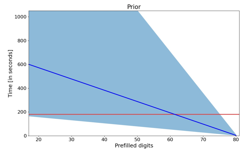
(a) Prior for the Sudoku experiment. This prior encodes the assumption that a Sudoku with 80 prefilled digits would be trivial to solve, and that the difficulty and uncertainty increases as there are fewer prefilled digits.

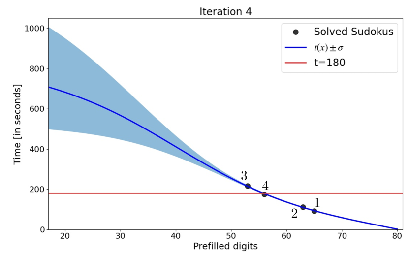
(b) 4th iteration of a FastBayesianContentAdaption playtrace.

Figure 1: A Sudoku playtrace. Once FBCA is deployed with an appropriate prior (a), the player is shown a Sudoku with 65 digits. In the case of this particular playtrace, the player took 92 seconds to complete it. Our approach then runs an iteration of the Bayesian Optimization, serving a level with 63 hints. Since this level is still too easy (111 seconds), the modified acquisition function $\beta^{180}_{\text{EI}}$ suggests a Sudoku with 53 digits, which takes the player 216 seconds to solve. Finally, a Sudoku with 55 hints is presented that takes the player 175 seconds to solve. The resulting model of the player at this fourth iteration of FBCA is presented in (b).

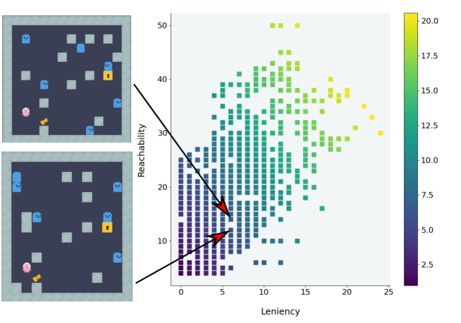
Figure 2: Prior creation for the Roguelike experiment. We pre-computed a corpus of levels for our Roguelike game and, for each one of them, we computed their leniency $l$ (amount of enemies) and reachability $r$ (sum of the length of the A* paths from the avatar to the key and from the key to the final goal). All optimizations of the roguelike experiment take place in the $(l,r)$ space this figure illustrates. We associated to each level a prior, built on the assumption that levels with low leniency and reachability could be solved in 1 second, and levels high leniency and reachability in 20 seconds.

IV Experimental Setup

Our approach for Fast Bayesian Content Adaption promises to be able to adjust contents in a design space $\mathcal{D}$ according to the behavior of the player. To test this approach we chose two domains: the puzzle Sudoku, and a simple Roguelike game.

IV-A Sudoku

A Sudoku puzzle (size 9$\times$9) requieres filling in the digits between 1 and 9 in grids of size 3$\times$3 such that no number appears more than once in its grid, row, and column. The difficulty of a Sudoku can be measured in terms of the number of prefilled digits, which ranges from 17 (resulting in a very difficult puzzle) to 80 (which is trivial). Thus, we settled on $\mathcal{D}=\{17,18,\dots,80\}$ as the design space for this domain.

To test our approach, we deployed a web app with an interface that serves Sudokus of varying amounts of prefilled digits $x\in\mathcal{D}$. We settled for a goal of $t_{g}=180$sec, instructed users to solve the puzzles as fast as they could, and initiated the player model with a linear prior $\mu_{0}(x)$ that interpolates the points (80, 3) and (17, 600) (see Fig. 1(a)). For this experiment, we used the RBF kernel $k_{\text{RBF}}$ and the modified Expected Improvement acquisition $\beta^{t_{g}}=\beta^{t_{g}}_{\text{EI}}$, and we computed this expectation using ancestral sampling (since $\log(t(x))\sim\text{GP}$) and Monte Carlo integration (see Sec. III).

We compare our FBCA approach with a binary search baseline which explores $\mathcal{D}$ by halving it, and jumping to the easy/difficult part according to the performance of the player. We also compared our approach with a linear regression policy for selecting the next Sudoku: we approximate player’s completion time starting with the same prior as with our approach and, once new data arrives, we fit a linear model to it in log-time space and present a sudoku that the model says will perform closest to $t_{g}$. Unfortunately, we were not able to gather enough playtraces to make significant statistical comparisons in the linear regression case, so our analysis will focus on the comparison between our approach and simple binary search. However, we present a short comparison between leveraging this linear regression model and deploying our FBCA system.

IV-B Roguelike

We also tested our approach in a simple Roguelike game, in which the player must navigate a level, grab a key and proceed to a final objective while avoiding enemies that move randomly. The player can move in all directions and when facing an enemy, can kill it (Fig. 2).

This domain is significantly different from Sudoku since difficulty is not as straight-forward to define and model, and it is also an instance of a roguelike game that players have not played prior. Two variables that influence the difficulty of a level are leniency $l$, defined as the number of enemies in the level; and reachability $r$, defined as the sum of the A* paths from the player’s avatar to the key and from the key to the goal. Using these, we define the as design space $\mathcal{D}=\{(l,r)\}\subseteq\mathbb{R}^{2}$.

Users are presented levels of the Roguelike game online, and are instructed to solve them as quickly as they can. In our optimizations, we target to find levels that take $t_{g}=10$ seconds.

We construct a prior $\mu_{0}(x)$ by computing a corpus of 399 randomly-generated levels $\mathcal{L}$ in the intervals $l\in[0,24]$ and $r\in[4,50]$. Levels were generated in an iterative process: first by sampling specifications such as height, width, and amount of enemies and randomly placing assets such that the A* path between the player and the goals are preserved, and then by mutating (adding/removing rows, columns, and assets) previously generated levels. We defined $\mu_{0}(x)$ by interpolating a plane in which a level with $l=0,r=4$ takes $1$ second to solve, and a level with $l=14,r=50$ would take 20 seconds to solve. Fig. 2 shows this prior, as well as example levels and their place in the design space.

For the GP, we chose a kernel $k$ that combines a linear assumption, as well as local interactions using the RBF kernel: $k=k_{\text{RBF}}+k_{\text{Linear}}$, together with the modified Upper Confidence Bounds acquisition function $\beta^{t_{g}}=\beta^{t_{g}}_{\text{UCB},\kappa}$ with $\kappa=0.05$. These hyperparameters (kernel shape and $\kappa$) were selected after several trial-and-error iterations of the experiment. Hyperparameters inside the kernels themselves were obtained by maximizing the likelihood w.r.t the data.

We compare our approach with two other methods: selecting levels completely at random from the corpus $\mathcal{L}$, and a Noisy Hill-climbing algorithm that starts in the center of $\mathcal{D}$, takes a random step (governed by normal noise) arriving at a new level $x$ and performance $t$, and consolidates $x$ as the new center for exploration if $t$ is closer to the goal $t_{g}$. When users enter the website and game, they are assigned one of these three approaches at random. These baselines were selected since methods for DDA discussed in Sec. II are either domain-specific, or they optimize for engagement and thus do not apply in this context.

V Results and Discussion

V-A Sudoku

We received a total of 288 unique playtraces for FBCA, and 94 unique playtraces using binary search. This discrepancy, however, is accounted for in the statistical tests we perform.

Figure 1 shows on the one hand the prior $\mu_{0}(x)$ we used for the fast adaption, and on the other the approximation $t(x)\sim\text{GP}$ after a player was presented with 4 different Sudokus, following Algorithm 1. The first Sudoku had 65 prefilled digits and was too easy for the player, who solved it in only 92 seconds. In the next iteration, the modified acquisition function $\beta^{180}_{\text{EI}}$ achieved its maximum over $\mathcal{D}=\{17,\dots,80\}$ at 63 hints. This Sudoku, however, also proved too easy for the player, who solved it in 111 seconds. The next Sudoku suggested by the system had 55 prefilled digits and took the player over 3 minutes to solve and, finally, at the 4th iteration, the system presented a Sudoku that took the player 175 seconds to solve, showing that our method was able to find (for this particular player) a puzzle with difficulty close to the target $t_{g}=180$ in only 4 iterations.

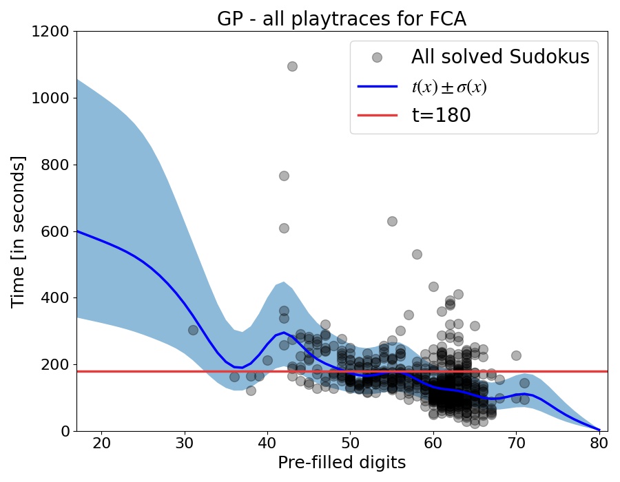
Figure 3: The average Sudoku player. This figure presents the result of fitting a Gaussian process to all the playtraces we gathered for Sudoku when testing the FBCA algorithm. The prior $\mu_{0}(x)$ presented in Fig. 1(a) was updated using an RBF kernel with data from 598 correctly-solved Sudokus, resulting in an approximation $t(x)$ of how long it would take an average player to solve a Sudoku with $x$ hints.

Iteration	$\mu_{e}^{\text{FBCA}}\pm\sigma$	$\mu_{e}^{\text{bin}}\pm\sigma$	$H_{0}$ rejected
1	72.5$\pm$ 47.5	135.9$\pm$ 266.4	yes ($p=0.04$)
2	76.9$\pm$ 94.6	122.3$\pm$ 202.6	no ($p=0.17$)
3	49.6$\pm$ 33.8	132.7$\pm$ 361.8	no ($p=0.22$)
4	47.6$\pm$ 66.7	39.5$\pm$ 33.2	no ($p=0.52$)
5	60.4$\pm$ 114.5	44.1$\pm$ 35.6	no ($p=0.45$)
6	36.5$\pm$ 34.9	72.6$\pm$ 106.5	no ($p=0.35$)
7	37.3$\pm$ 36.3	49.1$\pm$ 40.1	no ($p=0.50$)
8	29.9$\pm$ 29.6	79.8$\pm$ 79.4	no ($p=0.19$)
All	63.9 $\pm$ 67.3	110.5 $\pm$237.1	yes ($p=0.01$)

TABLE I: Mean absolute errors for the Sudoku experiment. This table presents the mean errors $\mu_{e}$ and their respective standard deviations. At each iteration, we consider all sudokus solved by users and their respective times. We compute the distance to the goal of the optimization (180 seconds), and we average them over the total amount of sudokus presented for said iteration. The mean error for FBCA $\mu_{e}^{\text{FBCA}}$ is significantly less than that for the binary search $\mu_{e}^{\text{bin}}$, which means that the null hypothesis $H_{0}:\mu_{e}^{\text{FBCA}}=\mu_{e}^{\text{bin}}$ is rejected according to a two-tailed $t$-test with acceptance rate of 0.05.

level #s	$\mu_{e}^{\text{FBCA}}$	$\mu_{e}^{\text{NH}}$	$\mu_{e}^{\text{rand}}$	$H_{0}^{\text{NH}}$ rejected	$H_{0}^{\text{rand}}$ rejected
$1\leq i<5$	3.66$\pm$ 3.48	5.76$\pm$ 5.63	7.09$\pm$ 6.73	yes ($p=0.01$)	yes ($p<0.01$)
$5\leq i<10$	3.65$\pm$ 3.94	4.88$\pm$ 4.98	6.28$\pm$ 6.03	no ($p=0.10$)	yes ($p<0.01$)
$10\leq i<15$	3.97$\pm$ 5.15	4.39$\pm$ 6.76	4.65$\pm$ 3.80	no ($p=0.72$)	no ($p=0.47$)
$15\leq i<20$	4.76$\pm$ 6.62	3.69$\pm$ 3.09	6.39$\pm$ 6.39	no ($p=0.41$)	no ($p=0.32$)
$20\leq i<25$	3.30$\pm$ 3.68	4.36$\pm$ 4.91	5.13$\pm$ 5.45	no ($p=0.42$)	no ($p=0.20$)
$25\leq i<30$	2.23$\pm$ 1.68	5.20$\pm$ 6.17	3.97$\pm$ 3.15	no ($p=0.07$)	no ($p=0.08$)
$30\leq i<35$	2.58$\pm$ 2.44	4.00$\pm$ 4.05	4.55$\pm$ 1.91	no ($p=0.29$)	no ($p=0.06$)
All	3.78$\pm$ 4.59	4.73$\pm$ 5.32	5.94$\pm$ 5.74	yes ($p=0.01$)	yes ($p<0.01$)

TABLE II: Mean absolute errors for the Roguelike experiment. This table presents the mean absolute error for FastBayesianContentAdaption (FBCA) $\mu_{e}^{\text{FBCA}}$, the Noisy Hill-climbing (NH) baseline $\mu_{e}^{\text{NH}}$, and for serving random levels $\mu_{e}^{\text{rand}}$. This data supports two claims: Our approach FBCA improves in its understanding of the player over time (which can be sensed from the fact that $\mu_{e}^{\text{FBCA}}$ decreases the more levels a player solves), and FBCA performs better than NH and serving random levels on average (since $\mu_{e}^{\text{FBCA}}$ is less than $\mu_{e}^{\text{NH}}$ and $\mu_{e}^{\text{rand}}$ in almost all intervals). While our approach performs significantly better when taking all iterations into account, in some instances this performance increase, while observable, is not significant. These results are also reported visually in Fig. 5

.

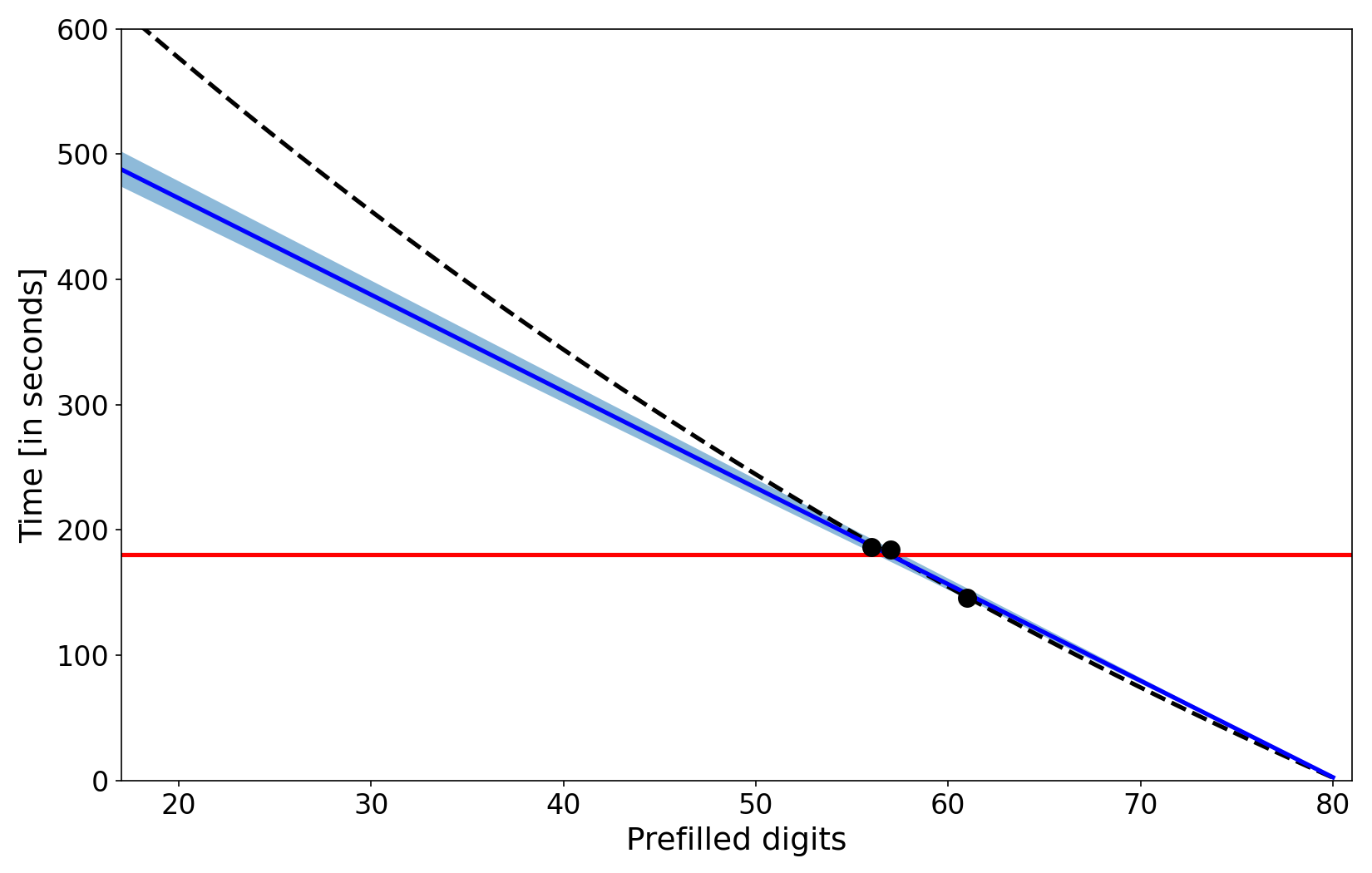
(a) Example: linear regression of log-time is enough.

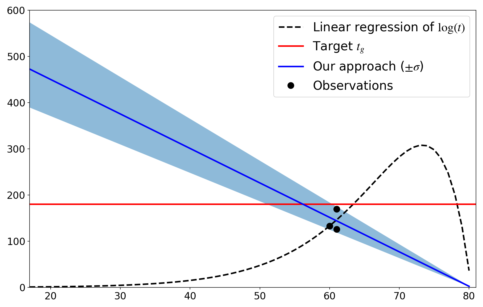
(b) Example: linear regression fails to show appropriate sudokus.

Figure 4: Gaussian Process Regression vs. Linear regression in Sudoku. Shown is a preliminary comparison of our approach against a greedy policy that models players time using linear regression in $\log(t)$ space. (a) shows an example in which this greedy policy was able to find a sudoku with the target time (with a playtrace of [145, 186, 184] seconds), while in (b) we see an example in which the linear regression fails to capture an adequate model of difficulty for the player (with a playtrace of [169, 132, 125] seconds). In both examples, our approach (that relies on Gaussian Process Regression with an RBF kernel) is able to capture a model of the player that decreases completion time w.r.t increasing hints. This seems to be a sensible model of difficulty, both intuitively and according to the result of fitting our approach with all (solved) sudoku playtraces (see Fig. 3)

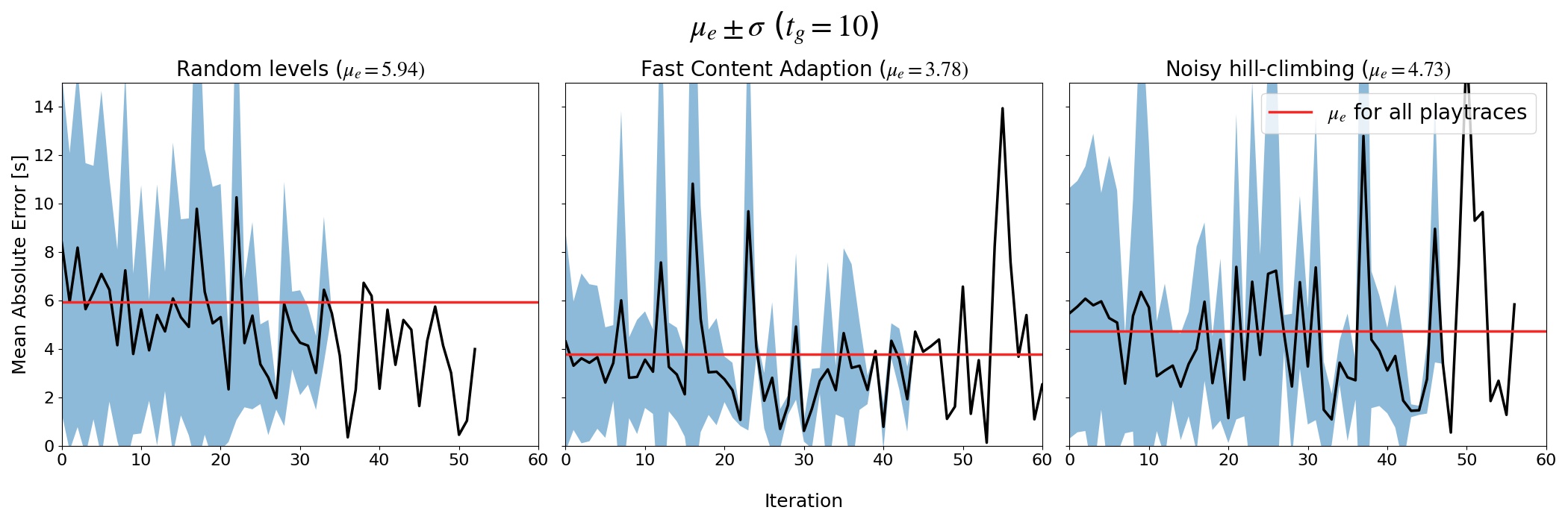
Figure 5: Mean absolute error for the Roguelike experiment. Shown is the average distance to the goal $t_{g}=10$ for three different approaches (presenting levels randomly, using Fast Bayesian Content Adaption, and using a baseline of Noisy Hill-climbing). Overall, we can see that the Bayesian optimization’s absolute mean error is decreasing, albeit with noise. The difference between the Bayesian Optimization and the other approaches is small (in the ballpark of 1 or 2 seconds) but significant. The blue shaded region represents $\pm\sigma$, and it disappears after e.g. 45 in the FBCA since, from that point onwards, we only have one playtrace.

To measure which approach performed better (between FBCA and binary search), we use the mean absolute error metric, defined as

$$\mu_{e}(\mathcal{T};t_{g})=\frac{1}{|\mathcal{T}|}\sum_{t\in\mathcal{T}}|t-t_{g}|,$$ (2)

this quantity measures how far, on average, the times recorded were from the goal time $t_{g}$. For brevity in the presentation, we will use the symbols $\mu_{e}^{\text{FBCA}}$ to stand for the mean absolute error of the times collected for the Bayesian experiment $\mathcal{T}_{\text{FBCA}}$ and goal $t_{g}=180$, and likewise for the binary search data with $\mu_{e}^{\text{bin}}$.

Table I shows the mean absolute error for the Sudoku experiment, segmented by the $i$th sudoku presented to the user. We only consider puzzles that were correctly solved, ignoring Sudokus solved in over 3000 seconds. According to the data for the first iteration, Sudokus with 65 hints (the starting point for FastBayesianContentAdaption) are closer to the goal of 3 minutes than the starting point of binary search on average. Both approaches appear to be getting closer to the goal the more Sudokus the player plays, ending with an average distance to the goal of about 30 seconds for FBCA in the best case ($i=8$) and of about 40 seconds in the binary search ($i=4$).

While these results have high variance, two-tailed $t$-tests that assume different group variances allow us to reject the null hypothesis $H_{0}:\mu_{e}^{\text{FBCA}}=\mu_{e}^{\text{bin}}$ (with a $p$-value of 0.01, less than the acceptance rate of 0.05) when including all the playtraces for both experiments. FBCA has a mean absolute error that almost halves the binary search one (with statistical significance). We hypothesize that this happens because the search in FBCA takes place around the easier levels, as is shown in Fig. 3. We assume this preference for easier puzzles is the result of a prior that favors easy levels and a variance that is more uncertain of harder levels. The same is not the case for the binary search; if a player solves the first Sudoku in less than 3 minutes, they are presented with a puzzle with only 33 prefilled digits next (which is significantly harder).

While we were not able to gather enough playtraces to perform significant statistical comparisons between our approach and using a greedy policy based on linear regression, we can anecdotally tell that there were cases in which a linear model of log-time failed to capture the player’s performance. In Fig. 4 we show two example playtraces that were gathered for the linear regression policy experiment. In the first one (Fig. 4(a)) we can see that using linear regression was enough to capture a model of the player and accurately present to them Sudokus that targeted the appropriate difficulty. On the other hand, Fig. 4(b) shows a critical example in which the predictions of simple linear regression state that sudokus with 17 hints are extremely easy. This seems to indicate that Gaussian Process Regression (with RBF kernels) is a better model for predicting completion log-time in this particular experiment.

V-B Roguelike

Players were assigned one of the three experiments discussed in Sec. IV-B at random when using our web application and were instructed to solve the levels they were presented as quickly as possible. We recorded a total of 18 unique playtraces for FBCA, 21 for the Noisy Hill-climbing, and 30 for the completely random approach. Like in the Sudoku experiment, our statistical tests are resilient to this discrepancy in sample sizes. In preparation for the data analysis, we removed all levels solved in over 60 seconds of time, since they are designed to be short, and a solved time of over a minute may indicate that the player got distracted.

Table II shows the mean absolute error (see Eq. (2)) for all three approaches, dividing the iterations in smaller intervals for ease of presentation and smoothing purposes. We see that the mean absolute error for FBCA ($\mu_{e}^{\text{FBCA}})$ decreases the more levels a player solves. This effect is to be expected since the underlying player model better approximates the player’s actual performance. Although the results have high variance, we can say with statistical confidence (using a two-tailed t-test with an acceptance rate of $0.05$) that FBCA performs better than Noisy Hill-climbing and serving completely random levels, but this is due to a small margin: of less than a second vs. NH, and two seconds vs. serving random levels. Fig. 5 shows the mean absolute error for all three methods, including one standard deviation and the average for all levels solved. Notice how the mean absolute error for all playtraces is lower for FBCA than for serving random levels, or Noisy Hill-climbing. We argue that the position of this mean error also indicates that the high spikes that can be seen in all approaches are outliers that could be explained by temporary distractions from the players.

VI Conclusions and Future Work

This paper presented a new approach, called Fast Bayesian Content Adaption (FBCA), with a focus on automatic difficulty adjustment in games. Our method maintains a simple model of the player, updates it as soon as data about the interaction between the user and the game arrives using Gaussian Processes, and uses a modified acquisition function to identify the next best level to present.

We tested FBCA in two domains: finding a Sudoku that takes 3 minutes to solve, and a level for a Roguelike game that takes 10 seconds to solve. Experiments that compare FBCA with simpler baselines in both domains show that our approach is able to find levels with target difficulty quickly and with significantly less distance to the target goal. While the results have a high variance, the mean error of FBCA is significantly lower than that of the baseline we compare to.

Our method thus provides an alternative for automatic difficulty adjustment that can, in only a few trials, learn which content in a design space elicits a particular target value (e.g. completion time) for a given player.

There are several avenues for future research: First, enforcing stronger assumptions about the monotonicity of the function that is being modeled in the Bayesian Optimization [25] might be beneficial if the content of the game is encoded in features that relate to difficulty directly (e.g. amount of enemies). Moreover, approaches in which the prior is automatically learned using artificial agents as proxies for humans could be explored [26]. The fact that our model assumes that the player does not improve over time could also be tackled in future research, by forgetting the initial parts of the playtrace using a sliding window. Finally, the features that make the contents of the design space difficult could be automatically learned by training generative methods (e.g. GANs or VAEs) and exploring the latent space of content they define [27, 28, 29, 30].

References

- [1] O. Pastushenko, “Gamification in education : dynamic difficulty adjustment and learning analytics,” in CHI PLAY 2019 - Extended Abstracts of the Annual Symposium on Computer-Human Interaction in Play, no. October, 2019.
- [2] R. Hunicke and V. Chapman, “AI for dynamic difficulty adjustment in games,” AAAI Workshop - Technical Report, vol. WS-04-04, pp. 91–96, 2004.
- [3] M. P. Silva, V. do Nascimento Silva, and L. Chaimowicz, “Dynamic difficulty adjustment on MOBA games,” Entertainment Computing, vol. 18, pp. 103–123, 2017.
- [4] A. E. Zook and M. O. Riedl, “A temporal data-driven player model for dynamic difficulty adjustment,” Proceedings of the 8th AAAI Conference on Artificial Intelligence and Interactive Digital Entertainment, AIIDE 2012, pp. 93–98, 2012.
- [5] S. Demediuk, M. Tamassia, W. L. Raffe, F. Zambetta, X. Li, and F. Mueller, “Monte Carlo tree search based algorithms for dynamic difficulty adjustment,” 2017 IEEE Conference on Computational Intelligence and Games, CIG 2017, pp. 53–59, 2017.
- [6] Y. Hao, Suoju He, Junping Wang, Xiao Liu, jiajian Yang, and Wan Huang, “Dynamic difficulty adjustment of game ai by mcts for the game pac-man,” in 2010 Sixth International Conference on Natural Computation, vol. 8, 2010, pp. 3918–3922.
- [7] M. Jennings-Teats, G. Smith, and N. Wardrip-Fruin, “Polymorph: Dynamic Difficulty Adjustment through level generation,” Workshop on Procedural Content Generation in Games, PC Games 2010, Co-located with the 5th International Conference on the Foundations of Digital Games, no. June 2010, pp. 2–6, 2010.
- [8] H.-S. Moon and J. Seo, “Dynamic difficulty adjustment via fast user adaptation,” in Adjunct Publication of the 33rd Annual ACM Symposium on User Interface Software and Technology, 2020, pp. 13–15.
- [9] A. Anthropy and N. Clark, A Game Design Vocabulary: Exploring the Foundational Principles Behind Good Game Design, 1st ed. Addison-Wesley Professional, 2014.
- [10] M. González-Duque, R. B. Palm, D. Ha, and S. Risi, “Finding game levels with the right difficulty in a few trials through intelligent trial-and-error,” in 2020 IEEE Conference on Games (CoG), 2020, pp. 503–510.
- [11] S. Xue, M. Wu, J. Kolen, N. Aghdaie, and K. A. Zaman, “Dynamic difficulty adjustment for maximized engagement in digital games,” 26th International World Wide Web Conference 2017, WWW 2017 Companion, pp. 465–471, 2017.
- [12] M. Zohaib, “Dynamic difficulty adjustment (DDA) in computer games: A review,” Advances in Human-Computer Interaction, vol. 2018, 2018.
- [13] R. Hunicke, “The case for dynamic difficulty adjustment in games,” ACM International Conference Proceeding Series, vol. 265, pp. 429–433, 2005.
- [14] J. Togelius, R. De Nardi, and S. M. Lucas, “Towards automatic personalised content creation for racing games,” Proceedings of the 2007 IEEE Symposium on Computational Intelligence and Games, CIG 2007, pp. 252–259, 2007.
- [15] N. Shaker, G. Yannakakis, and J. Togelius, “Towards automatic personalized content generation for platform games,” Proceedings of the 6th AAAI Conference on Artificial Intelligence and Interactive Digital Entertainment, AIIDE 2010, no. June 2014, pp. 63–68, 2010.
- [16] D. Thue, V. Bulitko, M. Spetch, and W. Eric, “Interactive storytelling: A player modelling approach,” Proceedings of the 3rd Artificial Intelligence and Interactive Digital Entertainment Conference, AIIDE 2007, no. January 2007, pp. 43–48, 2007.
- [17] A. Zook, E. Fruchter, and M. O. Riedl, “Automatic playtesting for game parameter tuning via active learning,” in Proceedings of the 9th International Conference on the Foundations of Digital Games, FDG 2014, Liberty of the Seas, Caribbean, April 3-7, 2014, M. Mateas, T. Barnes, and I. Bogost, Eds. Society for the Advancement of the Science of Digital Games, 2014. [Online]. Available: http://www.fdg2014.org/papers/fdg2014_paper_39.pdf
- [18] M. M. Khajah, B. D. Roads, R. V. Lindsey, Y.-E. Liu, and M. C. Mozer, “Designing engaging games using bayesian optimization,” in Proceedings of the 2016 CHI Conference on Human Factors in Computing Systems, ser. CHI ’16. New York, NY, USA: Association for Computing Machinery, 2016, p. 5571–5582. [Online]. Available: https://doi.org/10.1145/2858036.2858253
- [19] J. Snoek, H. Larochelle, and R. P. Adams, “Practical bayesian optimization of machine learning algorithms,” in Advances in Neural Information Processing Systems, F. Pereira, C. J. C. Burges, L. Bottou, and K. Q. Weinberger, Eds., vol. 25. Curran Associates, Inc., 2012, pp. 2951–2959. [Online]. Available: https://proceedings.neurips.cc/paper/2012/file/05311655a15b75fab86956663e1819cd-Paper.pdf
- [20] E. Brochu, V. M. Cora, and N. de Freitas, “A Tutorial on Bayesian Optimization of Expensive Cost Functions, with Application to Active User Modeling and Hierarchical Reinforcement Learning,” 2010. [Online]. Available: http://arxiv.org/abs/1012.2599
- [21] A. Cully, J. Clune, D. Tarapore, and J.-B. Mouret, “Robots that can adapt like animals,” Nature, vol. 521, no. 7553, pp. 503–507, May 2015. [Online]. Available: https://doi.org/10.1038/nature14422
- [22] B. Shahriari, K. Swersky, Z. Wang, R. P. Adams, and N. de Freitas, “Taking the human out of the loop: A review of bayesian optimization,” Proceedings of the IEEE, vol. 104, no. 1, pp. 148–175, 2016.
- [23] C. Rasmussen and C. Williams, Gaussian Processes for Machine Learning, ser. Adaptive Computation and Machine Learning. Cambridge, MA, USA: MIT Press, Jan. 2006.
- [24] F. Pedregosa, G. Varoquaux, A. Gramfort, V. Michel, B. Thirion, O. Grisel, M. Blondel, P. Prettenhofer, R. Weiss, V. Dubourg, J. Vanderplas, A. Passos, D. Cournapeau, M. Brucher, M. Perrot, and E. Duchesnay, “Scikit-learn: Machine learning in Python,” Journal of Machine Learning Research, vol. 12, pp. 2825–2830, 2011.
- [25] J. Riihimäki and A. Vehtari, “Gaussian processes with monotonicity information,” Journal of Machine Learning Research, vol. 9, pp. 645–652, 2010.
- [26] J. T. Kristensen, A. Valdivia, and P. Burelli, “Estimating player completion rate in mobile puzzle games using reinforcement learning,” in 2020 IEEE Conference on Games (CoG), 2020, pp. 636–639.
- [27] V. Volz, J. Schrum, J. Liu, S. M. Lucas, A. Smith, and S. Risi, “Evolving mario levels in the latent space of a deep convolutional generative adversarial network,” in Proceedings of the Genetic and Evolutionary Computation Conference, ser. GECCO ’18. New York, NY, USA: Association for Computing Machinery, 2018, p. 221–228. [Online]. Available: https://doi.org/10.1145/3205455.3205517
- [28] R. Rodriguez Torrado, A. Khalifa, M. Cerny Green, N. Justesen, S. Risi, and J. Togelius, “Bootstrapping conditional gans for video game level generation,” in 2020 IEEE Conference on Games (CoG), 2020, pp. 41–48.
- [29] M. C. Fontaine, R. Liu, A. Khalifa, J. Modi, J. Togelius, A. K. Hoover, and S. Nikolaidis, “Illuminating mario scenes in the latent space of a generative adversarial network,” 2020.
- [30] A. Sarkar, Z. Yang, and S. Cooper, “Conditional level generation and game blending,” in Proceedings of the Experimental AI in Games (EXAG) Workshop at AIIDE, 2020.