Parallel Attention Network with Sequence Matching for Video Grounding

Abstract

Given a video, video grounding aims to retrieve a temporal moment that semantically corresponds to a language query. In this work, we propose a Parallel Attention Network with Sequence matching (SeqPAN) to address the challenges in this task: multi-modal representation learning, and target moment boundary prediction. We design a self-guided parallel attention module to effectively capture self-modal contexts and cross-modal attentive information between video and text. Inspired by sequence labeling tasks in natural language processing, we split the ground truth moment into begin, inside, and end regions. We then propose a sequence matching strategy to guide start/end boundary predictions using region labels. Experimental results on three datasets show that SeqPAN is superior to state-of-the-art methods. Furthermore, the effectiveness of the self-guided parallel attention module and the sequence matching module is verified.

1 Introduction

Video grounding is a fundamental and challenging problem in vision-language understanding research area Hu et al. (2019); Yu et al. (2019); Zhu and Yang (2020). It aims to retrieve a temporal video moment that semantically corresponds to a given language query, as shown in Figure 1. This task requires techniques from both computer vision Tran et al. (2015); Shou et al. (2016); Feichtenhofer et al. (2019), natural language processing Yu et al. (2018); Yang et al. (2019), and more importantly, the cross-modal interactions between the two. Many existing solutions Chen et al. (2018); Liu et al. (2018a); Xu et al. (2019) tackle video grounding problem with proposal-based approach. This approach generates proposals with pre-set sliding windows or anchors, computes the similarity between the query and each proposal. The proposal with highest score is selected as the answer. These methods are sensitive to the quality of proposals and are inefficient because all proposal-query pairs are compared. Recently, several one-stage proposal-free solutions Chen et al. (2019); Lu et al. (2019a); Mun et al. (2020) are proposed to directly predict start/end boundaries of target moments, through modeling video-text interactions. Our solution, SeqPAN, is a proposal-free method; hence our key focuses are video-text interaction modeling and moment boundary prediction.

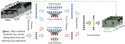
Figure 1: The overview of our procedures for video grounding, with an example of retrieving the temporal moment from an untrimmed video by a given language query.

Video-text interaction modeling. In order to model video-text interaction, various attention-based methods have been proposed Gao et al. (2017); Yuan et al. (2019a); Mun et al. (2020). In particular, transformer block Vaswani et al. (2017) is widely used in vision-language tasks and proved to be effective for multimodal learning Tan and Bansal (2019); Lu et al. (2019b); Su et al. (2020); Li et al. (2020). In video grounding task, fine-grain scale unimodal representations are important to achieve good localization performance. However, existing solutions do not refine unimodal representations of video and text when doing cross-modal reasoning, and thus limit the performance.

To better capture informative features for multi-modalities, we encode both self-attentive contexts and cross-modal interactions from video and query. That is, instead of solely relying on sophisticated cross-modal learning as in most existing studies, we learn both intra- and inter-modal representations simultaneously, with improved attention modules.

Moment boundary prediction. In terms of the length, target moment is usually a very small portion of the video, making positive (frames in target moment) and negative (frames not in target moment) samples imbalanced. Further, we aim to predict the exact start/end boundaries (i.e., two video frames) of the target moment. If we view from the space of video frames, sparsity is a major concern, e.g., catching two frames among thousands. Recent studies attempt to address this issue by auxiliary objectives, e.g., to discriminate whether each frame is foreground (positive) or background (negative) Yuan et al. (2019b); Mun et al. (2020), or to regress distances of each frame within target moment to ground truth boundaries Lu et al. (2019a); Zeng et al. (2020). However, the “sequence” nature of frames or videos is not considered.

We emphasize the “sequence” nature of video frames and adopt the concept of sequence labeling in NLP to video grounding. We use named entity recognition (NER) Lample et al. (2016); Ma and Hovy (2016) as an example sequence labeling task for illustration in Figure 2. Video grounding is to retrieve a sequence of frames with start/end boundaries of target moment from video. This is analogous to extract a multi-word named entity from a sentence. The main difference is that, words are discrete, so word annotations (i.e., B, I, E, and O tags) in sentence are discrete. In contrast, video is continuous and the changes between consecutive frames are smooth. Hence, it is difficult (and also not necessary) to precisely annotate each frame. We relax the annotations on video sequence by specifying video regions, instead of frames. With respect to the target moment, we label B, I, E and O (BIEO) regions on video (see Figure 3) and introduce label embeddings to model these regions.

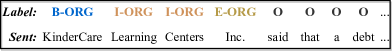
Figure 2: An example of the annotations in NER, where “ORG” is for “Organization”, “B”, “I” and “E” denote the begin, inside and end of the organization entity, respectively.

Our contributions. In this research, we propose a Parallel Attention Network with Sequence matching (SeqPAN) for video grounding task. We first design a self-guided parallel attention (SGPA) module to capture both self- and cross-modal attentive information for each modality simultaneously. In SGPA module, a cross-gating strategy with self-guided head is further used to fuse self- and cross-modal representations. We then propose a sequence matching (sq-match) strategy, to identify BIEO regions in video. The label embeddings are incorporated to represent label of frames in each region for region recognition. The sq-match guides SeqPAN to search for boundaries of target moment within constrained regions, leading to more precise localization results. Experimental results on three benchmarks demonstrate that both SGPA and sq-match consistently improve the performance; and SeqPAN surpasses the state-of-the-art methods.

2 Related Work

Existing solutions to video grounding are roughly categorized into proposal-based and proposal-free frameworks. In proposal-based framework, common structures include ranking and anchor-based methods. Ranking-based methods Liu et al. (2018b); Hendricks et al. (2017, 2018); Chen and Jiang (2019); Ge et al. (2019); Zhang et al. (2019b) solve this task with two-stage propose-and-rank pipeline, which first generates proposals and then uses multimodal matching to retrieve most similar proposal for a query. Anchor-based methods Chen et al. (2018); Yuan et al. (2019a); Zhang et al. (2019c); Wang et al. (2020b) sequentially assign each frame with multiscale temporal anchors and select the anchor with highest confidence as the result. However, these methods are sensitive to the proposal quality; and comparison of all proposal-query pairs is computational expensive and inefficient.

Proposal-free framework includes regression and span-based methods. Regression-based methods Yuan et al. (2019b); Lu et al. (2019a); Chen et al. (2020a, b) tackle video grounding by learning cross-modal interactions between video and query, and directly regressing temporal time of target moments. Span-based methods Ghosh et al. (2019); Rodriguez et al. (2020); Zhang et al. (2020a); Lei et al. (2020); Zhang et al. (2021) address video grounding by borrowing the concept of extractive question answering Seo et al. (2017); Huang et al. (2018), and to predict the start and end boundaries of target moment directly.

In addition, there are several works He et al. (2019); Wang et al. (2019); Cao et al. (2020); Hahn et al. (2020); Wu et al. (2020a, b) that formulate this task as a sequential decision-making problem and adopt reinforcement learning to observe candidate moments conditioned on queries. Other methods, e.g., weakly supervised learning methods Mithun et al. (2019); Lin et al. (2020); Wu et al. (2020a), 2D map model of temporal relations between video moments Zhang et al. (2020b), ensemble of top-down and bottom-up methods Wang et al. (2020a), joint learning video-level matching and moment-level localization Shao et al. (2018), have also been explored. Some works Shao et al. (2018); Cao et al. (2020); Liu et al. (2020); Wang et al. (2020a) use either additional resources/features or different evaluation metrics, so their results are not directly comparable with many others, including ours.

3 Proposed Method

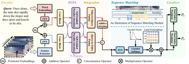
Figure 3: The architecture of the Parallel Attention Network with Sequence Matching (SeqPAN) for video grounding.

Let $V=[f_{t}]_{t=0}^{T-1}$ be an untrimmed video with $T$ frames; $Q=[q_{j}]_{j=0}^{M-1}$ be a language query with $M$ words; $t^{s}$ and $t^{e}$ denote start and end time point of ground-truth temporal moment. We define and tackle video grounding task in feature spaces. Specifically, we split the given video $V$ into $N$ clip units, and use pre-trained feature extractor to encode them into visual features $\bm{V}=[\bm{v}_{i}]_{i=0}^{N-1}\in\mathbb{R}^{d_{v}\times N}$, where $d_{v}$ is visual feature dimension. Then the $t^{s(e)}$ are mapped to the corresponding indices $i^{s(e)}$ in the feature sequence, where $0\leq i^{s}\leq i^{e}\leq N-1$. For the query $Q$, we encode words with pre-trained word embeddings as $\bm{Q}=[\bm{w}_{j}]_{j=0}^{M-1}\in\mathbb{R}^{d_{w}\times M}$, where $d_{w}$ is word dimension. Given the pair of $(\bm{V},\bm{Q})$ as input, video grounding aims to localize a temporal moment starting at $i^{s}$ and ending at $i^{e}$.

3.1 The SeqPAN Model

The overall architecture of the proposed SeqPAN model is shown in Figure 3. Next, we present each module of SeqPAN in detail.

3.1.1 Encoder Module

Given visual features $\bm{V}\in\mathbb{R}^{d_{v}\times N}$ of the video and word embeddings $\bm{Q}\in\mathbb{R}^{d_{w}\times M}$ of the language query, we map them into the same dimension $d$ with two FFNs, respectively. The encoder module mainly encodes the individual modality separately. As position encoding offers a flexible way to embed a sequence, when the sequence order matters, we first incorporate a position embedding to every input of both video and query sequences. Then, we adopt stacked 1D convolutional block to learn representations by carrying knowledge from neighbor tokens. The encoded representations are written as:

$$\bm{V^{\prime}} =\mathtt{ConvBlock}(\mathtt{FFN_{v}}(\bm{V})+\bm{E}_{p})$$ (1)

$$\bm{Q^{\prime}} =\mathtt{ConvBlock}(\mathtt{FFN_{q}}(\bm{Q})+\bm{E}_{p})$$

where $\bm{V^{\prime}}\in\mathbb{R}^{d\times N}$ and $\bm{Q^{\prime}}\in\mathbb{R}^{d\times M}$; $\bm{E}_{p}$ denotes the positional embeddings. Both position embeddings and convolutional block are shared by the video and text features.

3.1.2 Self-Guided Parallel Attention Module

A self-guided parallel attention (SGPA) module (see Figure 4) is proposed to improve multimodal representation learning. Compared with standard transformer (TRM) encoder, SGPA uses two parallel multi-head attention blocks to learn both uni-modal and cross-modal representations simultaneously, and merge them with a cross-gating strategy. Taking video modality as an example, the attention process is computed as:

$$\bm{\hat{V}}_{\text{S}}=V_{V}\cdot\sigma_{s}\Big{(}\frac{Q^{\top}_{V}K_{V}}{\sqrt{d}}\Big{)}$$ (2)

$$\bm{\hat{V}}_{\text{C}}=V_{Q}\cdot\sigma_{s}\Big{(}\frac{Q^{\top}_{V}K_{Q}}{\sqrt{d}}\Big{)}$$

where $\sigma_{s}$ denotes Softmax function; $Q_{V}$, $K_{V}$ and $V_{V}$ are the linear projections of $\bm{V^{\prime}}$; $Q_{Q}$, $K_{Q}$ and $V_{Q}$ are linear projections of $\bm{Q^{\prime}}$; $\bm{\hat{V}}_{\text{S}}$ encodes the self-attentive contexts within video modality; and $\bm{\hat{V}}_{\text{C}}$ integrates information from query modality according to cross-modal attentive relations. The self- and cross-modal representations are then merged together by a cross-gating strategy:

$$\bm{\hat{V}}=\sigma\big{(}\mathtt{FFN}(\bm{\hat{V}}_{\text{C}})\big{)}\odot\bm{\hat{V}}_{\text{S}}+\sigma\big{(}\mathtt{FFN}(\bm{\hat{V}}_{\text{S}})\big{)}\odot\bm{\hat{V}}_{\text{C}}$$ (3)

where $\sigma$ denotes Sigmoid function and $\odot$ represents Hadamard product. The cross-gating explicitly interacts features obtained from the self- and cross-attention encoders to ensure both are fully utilized, instead of relying on only one of them. Finally, we employ a self-guided head to implicitly emphasize the informative representations by measuring the confidence of each element in $\bm{\hat{V}}$ as:

$$\bm{\bar{V}}=\sigma\big{(}\mathtt{FFN}_{\sigma}(\bm{\hat{V}})\big{)}\odot\mathtt{FFN}(\bm{\hat{V}})$$ (4)

The refined representations $\bm{\bar{Q}}$ for the query modality are obtained in a similar manner (e.g., swapping visual and query features).

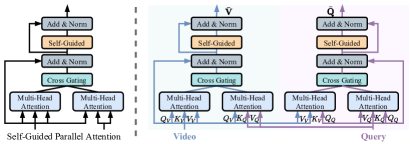
Figure 4: Self-Guided Parallel Attention (SGPA). Left: the structure of SGPA; Right: the parallel streams of encoding visual and textual inputs.

3.1.3 Video-Query Integration Module

This module further enhances the cross-modal interactions between visual and textual features. It utilizes context-query attention (CQA) strategy Yu et al. (2018) and aggregates text information for each visual element (see Figure 3). Given $\bm{\bar{V}}$ and $\bm{\bar{Q}}$, CQA first computes the similarities, $\mathcal{S}\in\mathbb{R}^{N\times M}$, between each pair of $\bm{\bar{V}}$ and $\bm{\bar{Q}}$ features. Then two attention weights are derived by $\mathcal{A}_{\text{VQ}}=\mathcal{S}_{r}\cdot\bm{\bar{Q}}^{\top}$ and $\mathcal{A}_{\text{QV}}=\mathcal{S}_{r}\cdot\mathcal{S}^{\top}_{c}\cdot\bm{\bar{V}}^{\top}$, where $\mathcal{S}_{r}$/$\mathcal{S}_{c}$ are row-/column-wise normalization of $\mathcal{S}$ by Softmax. The query-aware video representations $\bm{V}^{Q}$ is computed by:

$$\bm{V}^{Q}=\mathtt{FFN}\big{(}[\bm{\bar{V}};\mathcal{A}_{\text{VQ}}^{\top};\bm{\bar{V}}\odot\mathcal{A}_{\text{VQ}}^{\top};\bm{\bar{V}}\odot\mathcal{A}_{\text{QV}}^{\top}]\big{)}$$ (5)

where $\bm{V}^{Q}\in\mathbb{R}^{d\times N}$. Similarly, video-aware query representations $\bm{Q}^{V}\in\mathbb{R}^{d\times M}$ can be derived by swapping visual and textual inputs in CQA module. Then we encode $\bm{Q}^{V}$ into sentence representation $\bm{q}$ with additive attention Bahdanau et al. (2015) and concatenate it with each element of $\bm{V}^{Q}$ as $\bm{H}=[\bm{h}_{1},\dots,\bm{h}_{n}]$, where $\bm{h}_{i}=[\bm{v}_{i}^{Q};\bm{q}]$. Finally, the query-attended visual representation is computed as $\bm{\bar{H}}=\mathtt{FFN}(\bm{H})\in\mathbb{R}^{d\times N}$.

3.1.4 Sequence Matching Module

As illustrated in Figure 3, we considers the frames within ground truth moment and several neighboring frames as foreground, while the rest as background. Then, we split the foreground into Begin, Inside, and End regions. For simplicity, we assign each region a label, i.e., “B-M” for begin, “I-M” for inside, “E-M” for end region, and “O” for background. B-M/E-M explicitly indicate potential positions of the start/end boundaries. We also specify orthogonal label embeddings $\bm{E}_{\text{lab}}\in\mathbb{R}^{d\times 4}$ to represent those labels, and to infuse label information into visual features after region label predictions.

Note our approach is different from Lin et al. (2018) on temporal action proposal generation task, where the target proposal is split into start, centre, and end regions. The probability of a frame belonging to each of three regions is predicted separately in a regression manner, leading to three separate probability sequences, one for each region. The maximum probabilities in the sequences are used to guide proposal generations. In contrast, we formulate matching process as a multi-class classification problem and predict a concrete region label for each frame, i.e., same as a sequence labeling task in NLP. Label embeddings are then assigned to the frames based on the labels of the predicted region.

A straightforward solution to predict the confidence of an element belonging to each region is multi-class classifier:

$$\bm{H}_{\text{seq}}=\mathtt{FFN}_{\text{seq}}(\bm{\bar{H}}),\;\;\bm{S}_{\text{seq}}=\sigma_{s}(\bm{H}_{\text{seq}})\in\mathbb{R}^{4\times N}$$ (6)

where $\bm{S}_{\text{seq}}$ encodes the probabilities of each visual element in different regions. Then label index with highest probability from $\bm{S}_{\text{seq}}$ is selected to represent the predicted label for each visual element:

$$\bm{L}_{\text{lab}}=[\arg\max(\bm{S}^{j}_{\text{seq}})]_{j=0}^{N-1}\in\mathbb{R}^{N}$$ (7)

However, a major issue here is that Eq. 7 needs to sample from a discrete probability distribution, which makes the back-propagation of gradients through $\bm{S}_{\text{seq}}$ in Eq. 6 infeasible for optimizer. To make back-propagation possible, we adopt the Gumbel-Max Gumbel (1954); Maddison et al. (2014) trick to re-formulate Eq. 7 as:

$$\bm{\hat{L}}_{\text{lab}}=\big{[}\mathtt{Onehot}(\arg\max(\bm{H}^{j}_{\text{seq}}+\bm{g}))\big{]}_{j=0}^{N-1}$$ (8)

where $\bm{\hat{L}}_{\text{lab}}\in\mathbb{R}^{4\times N}$. Then, we utilize the Gumbel-Softmax Jang et al. (2017); Maddison et al. (2017) to relax the $\arg\max$ so as to make Eq. 8 being differentiable. Formally, we use Eq. 9 to approximate Eq. 8 as:

$$\bm{\bar{L}}_{\text{lab}}=\sigma_{s}\big{(}(\bm{H}_{\text{seq}}+\bm{g})/\tau\big{)}\in\mathbb{R}^{4\times N}$$ (9)

where $\tau$ is annealing temperature. As $\tau\to 0^{+}$, $\bm{\bar{L}}_{\text{lab}}\approx\bm{\hat{L}}_{\text{lab}}$, while $\tau\to\infty$, each element in $\bm{\bar{L}}_{\text{lab}}$ will be the same and the approximated distribution will be smooth. Note we use Eq. 8 during forward pass while Eq. 9 for backward pass to allow gradient back-propagation. As the result, the embedding lookup process is differentiable and the label-attended visual representations is derived as:

$$\bm{\widetilde{H}}=\bm{E}_{\text{lab}}\cdot\bm{\hat{L}}_{\text{lab}}+\bm{\bar{H}}$$ (10)

The training objective is defined as:

$$\mathcal{L}_{\text{seq}}=f_{\text{XE}}(\bm{\bar{L}}_{\text{lab}},\bm{Y}_{\text{lab}})+\|\bm{E}_{\text{lab}}^{\top}\bm{E}_{\text{lab}}\odot(\bm{1}-\bm{I})\|_{\text{F}}^{2}$$ (11)

where $\bm{Y}_{\text{lab}}$ denotes the ground truth sequence labels, $\bm{1}$ is the matrix with all elements being $1$ and $\bm{I}$ is the identity matrix. The second term in Eq. 11 is the orthogonal regularization Brock et al. (2019), which ensures $\bm{E}_{\text{lab}}$ to keep the orthogonality.

3.1.5 Localization Module

Finally, we present a conditioned localizer to predict the start and end boundaries of the target moment. The localizer consists of two stacked transformer blocks and two FFNs. The scores of start and end boundaries are calculated as:

$$\bm{H}_{\text{s}}=\mathtt{TRM}_{s}(\bm{\widetilde{H}}), \;\bm{S}_{s}=\bm{W}_{s}[\bm{H}_{\text{s}};\bm{\widetilde{H}}]+\bm{b}_{s}$$ (12)

$$\bm{H}_{\text{e}}=\mathtt{TRM}_{e}(\bm{H}_{\text{s}}), \;\bm{S}_{e}=\bm{W}_{e}[\bm{H}_{\text{e}};\bm{\widetilde{H}}]+\bm{b}_{e}$$

where $\bm{S}_{s/e}\in\mathbb{R}^{N}$. $\bm{W}_{s/e}$ and $\bm{b}_{s/e}$ are the weight and bias of start/end FFNs, respectively. Note the representations of end boundary ($\bm{H}_{\text{e}}$) are conditioned on that of start boundary ($\bm{H}_{\text{s}}$) to ensure the predicted end boundary is always after start boundary. Then, the probability distributions of start/end boundaries are computed by $\bm{P}_{s/e}=\mathtt{Softmax}(\bm{S}_{s/e})\in\mathbb{R}^{N}$. The training objective is:

$$\mathcal{L}_{\text{loc}}=\frac{1}{2}\times\big{[}f_{\text{XE}}(\bm{P}_{s},\bm{Y}_{s})+f_{\text{XE}}(\bm{P}_{e},\bm{Y}_{e})\big{]}$$ (13)

where $f_{\text{XE}}$ is cross-entropy function, $\bm{Y}_{s/e}$ is one-hot labels for start/end ($i^{s}$/$i^{e}$) boundaries.

3.2 Training and Inference

The overall training loss of SeqPAN is: $\mathcal{L}=\mathcal{L}_{\text{loc}}+\mathcal{L}_{\text{seq}}$, to be minimized during the training process. During inference, the predicted start and end boundaries of a given video-query pair are generated by maximizing the joint probability as:

$$(\hat{i}^{s},\hat{i}^{e})= \arg\max_{\hat{a}^{s},\hat{a}^{e}}\bm{P}_{s}(\hat{a}^{s})\times\bm{P}_{e}(\hat{a}^{e})$$ (14)

s.t.: $$0\leq\hat{i}^{s}\leq\hat{i}^{e}\leq N-1$$

where $\hat{i}^{s}$ and $\hat{i}^{e}$ are the best start and end boundaries of predicted moment for the given video-query pair. Let $\mathcal{T}$ be the duration of given video, the predicted start/end time are computed by $\hat{t}^{s(e)}=\hat{i}^{s(e)}/(N-1)\times\mathcal{T}$. With the predicted $(\hat{t}^{s},\hat{t}^{e})$ and ground truth $(t^{s},t^{e})$ time intervals, the measure, temporal intersection over union (IoU), is computed as:

$$\text{IoU}=\max\Big{(}0,\frac{t_{\text{min}}^{e}-t_{\text{max}}^{s}}{t_{\text{max}}^{e}-t_{\text{min}}^{s}}\Big{)}\in[0,1]$$ (15)

where $t_{\min/\max}^{s(e)}=\min/\max(\hat{t}^{s(e)},t^{s(e)})$.

4 Experiments

4.1 Experimental Setting

Datasets. We conduct the experiments on three benchmark datasets: Charades-STA Gao et al. (2017), ActivityNet Captions Krishna et al. (2017) and TACoS Regneri et al. (2013). Charades-STA, collected by Gao et al. (2017) from Charades Sigurdsson et al. (2016) dataset, contains $16,128$ annotations (i.e., moment-query pairs), where $12,408$ and $3,720$ annotations are for train and test. ActivityNet Captions (ANetCaps) contains $20$K videos taken from ActivityNet Heilbron et al. (2015) dataset. We follow the setup in Chen et al. (2020a); Lu et al. (2019a); Wu et al. (2020b); Yuan et al. (2019b); Zhang et al. (2020a) with $37,421$ and $17,505$ annotations for train and test. TACoS contains $127$ cooking activities videos from Rohrbach et al. (2012). We follow Gao et al. (2017) with $10,146$, $4,589$, and $4,083$ annotations are used for train, validation, and test, respectively.

Evaluation Metric. (i) “$\text{R@}n,\text{IoU=}\mu$”, which denotes the percentage of test samples that have at least one result whose IoU with ground-truth is larger than $\mu$ in top-$n$ predictions; (ii) “mIoU”, which denotes the average IoU over all test samples. We set $n=1$ and $\mu\in\{0.3,0.5,0.7\}$.

Implementation Details. We follow Ghosh et al. (2019); Mun et al. (2020); Rodriguez et al. (2020); Zhang et al. (2020a) and use 3D ConvNet pre-trained on Kinetics dataset Carreira and Zisserman (2017) to extract RGB visual features from videos; then we downsample the feature sequence to a fixed length. The query words are lowercased and initialized with GloVe Pennington et al. (2014) embedding. We set hidden dimension $d$ to $128$; SGPA blocks to $2$; annealing temperature to $0.3$; and heads in multi-head attention to $8$; Adam Kingma and Ba (2015) optimizer with batch size of $16$ and learning rate of $0.0001$ is used for training.

More details of dataset statistics and the hyper-parameter settings are summarized in Appendix.

Methods	$\text{R@}1,\text{IoU}=\mu$			mIoU
	$\mu=0.3$	$\mu=0.5$	$\mu=0.7$
DEBUG	54.95	37.39	17.69	36.34
ExCL	61.50	44.10	22.40	-
MAN	-	46.53	22.72	-
SCDM	-	54.44	33.43	-
CBP	-	36.80	18.87	-
GDP	54.54	39.47	18.49	-
2D-TAN	-	39.81	23.31	-
TSP-PRL	-	45.30	24.73	40.93
TMLGA	67.53	52.02	33.74	-
VSLNet	70.46	54.19	35.22	50.02
DRN	-	53.09	31.75	-
LGI	72.96	59.46	35.48	-
SeqPAN	73.84	60.86	41.34	53.92

Table 1: Comparison with SOTA methods on Charades-STA.

Methods	$\text{R@}1,\text{IoU}=\mu$			mIoU
	$\mu=0.3$	$\mu=0.5$	$\mu=0.7$
DEBUG	55.91	39.72	-	39.51
ExCL	63.00	43.60	24.10	-
SCDM	54.80	36.75	19.86	-
CBP	54.30	35.76	17.80	-
GDP	56.17	39.27	-	39.80
2D-TAN	59.45	44.51	27.38	-
TSP-PRL	56.08	38.76	-	39.21
TMLGA	51.28	33.04	19.26	-
VSLNet	63.16	43.22	26.16	43.19
DRN	-	45.45	24.36	-
LGI	58.52	41.51	23.07	-
SeqPAN	61.65	45.50	28.37	45.11

Table 2: Comparison with SOTA methods on ANetCaps.

Methods	$\text{R@}1,\text{IoU}=\mu$			mIoU
	$\mu=0.3$	$\mu=0.5$	$\mu=0.7$
TGN	21.77	18.90	-	-
ACL	24.17	20.01	-	-
DEBUG	23.45	11.72	-	16.03
SCDM	26.11	21.17	-	-
CBP	27.31	24.79	19.10	21.59
GDP	24.14	13.90	-	16.18
TMLGA	24.54	21.65	16.46	-
VSLNet	29.61	24.27	20.03	24.11
DRN	-	23.17	-	-
SeqPAN	31.72	27.19	21.65	25.86
2D-TAN	37.29	25.32	-	-
SeqPAN	48.64	39.64	28.07	37.17

Table 3: Comparison with SOTA methods on TACoS.

Methods	$\text{R@}1,\text{IoU}=\mu$
	$\mu=0.3$	$\mu=0.5$	$\mu=0.7$
Charades-STA
Se-TRM	68.84 (0.46)	51.92 (0.54)	34.58 (0.18)
Co-TRM	69.03 (0.49)	52.34 (0.50)	35.07 (0.32)
SGPA	69.47 (0.32)	54.63 (0.43)	36.36 (0.24)
ActivityNet Captions
Se-TRM	57.64 (0.38)	40.76 (0.35)	25.10 (0.30)
Co-TRM	57.39 (0.29)	40.55 (0.45)	24.85 (0.47)
SGPA	58.40 (0.31)	41.72 (0.19)	26.07 (0.16)

Table 4: SGPA vs. standard transformers on Charades-STA and ANetCaps. Se-TRM is the transformer block with single modality inputs, and Co-TRM Tan and Bansal (2019); Lu et al. (2019b); Lei et al. (2020); Li et al. (2020) is with dual modality inputs. Scores in brackets are standard deviation.

4.2 Comparison with State-of-the-Arts

We compare SeqPAN with the following state-of-the-arts. 1) Proposal-based methods: TGN Chen et al. (2018), ACL Ge et al. (2019), CBP Wang et al. (2020b), SCDM Yuan et al. (2019a), MAN Zhang et al. (2019a); 2) Proposal-free methods: DEBUG Lu et al. (2019a), ExCL Ghosh et al. (2019), VSLNet Zhang et al. (2020a), GDP Chen et al. (2020a), LGI Mun et al. (2020), TMLGA Rodriguez et al. (2020), DRN Zeng et al. (2020); 3) Others: TSP-PRL Wu et al. (2020b) and 2D-TAN Zhang et al. (2020b). The best results are in bold and the second bests are in italic. In all result tables, the scores of compared methods are reported in the corresponding works.

The results on the Charades-STA are summarized in Table 1. SeqPAN surpasses all baselines and achieves the highest scores over all metrics. Observe that the performance improvements of SeqPAN are more significant under more strict metrics. The results show that SeqPAN can produce more precise localization results. For instance, compared to LGI, SeqPAN achieves $5.86\%$ absolute improvement by “R@1, IoU=0.7”, and $1.40\%$ by “R@1, IoU=0.5”. Table 2 reports the results on ANetCaps. SeqPAN is superior to baselines and achieves the best performance on “R@1, IoU=0.7” and mean IoU. As reported in Table 3, similar observations hold on TACoS. Note 2D-TAN Zhang et al. (2020b) pre-processes the TACoS dataset, making it is slightly different from the original one. We also conduct experiments on their version for a fair comparison. SeqPAN outperforms the baselines over all evaluation metrics on both versions.

Method	sq-match		Charades-STA				ActivityNet Captions
			$\text{R@}1,\text{IoU}=\mu$			mIoU	$\text{R@}1,\text{IoU}=\mu$			mIoU
	$G$	$\bm{E}_{\text{lab}}$	$\mu=0.3$	$\mu=0.5$	$\mu=0.7$		$\mu=0.3$	$\mu=0.5$	$\mu=0.7$
SeqPAN w/ fb-match	-	-	70.27(0.75)	56.96(0.46)	38.95(0.27)	51.84(0.40)	59.99(0.25)	43.71(0.19)	26.72(0.29)	43.23(0.23)
SeqPAN w/o sq-match	✘	✘	69.62(0.54)	55.29(0.30)	36.71(0.48)	51.13(0.25)	59.03(0.35)	42.65(0.32)	26.29(0.13)	42.51(0.36)
SeqPAN w/ Gumbel	✔	✘	71.64(0.64)	57.61(0.26)	39.26(0.31)	52.15(0.45)	59.74(0.42)	43.85(0.35)	27.12(0.20)	43.69(0.24)
SeqPAN	✔	✔	72.70(0.51)	60.15(0.50)	41.02(0.36)	53.19(0.38)	61.12(0.39)	45.09(0.37)	27.97(0.27)	44.77(0.23)

Table 5: Ablation studies of sequence matching strategy in SeqPAN, where the values in bracket denote standard deviation.

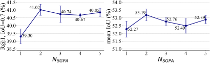
(a) Charades-STA

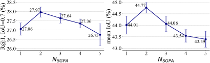
(b) ActivityNet Captions

Figure 5: The impact of SGPA block numbers ($N_{\text{SGPA}}$) on Charades-STA and ANetCaps.

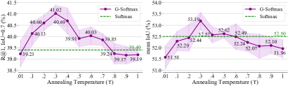
(a) Charades-STA

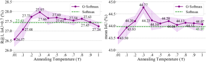
(b) ActivityNet Captions

Figure 6: The impact of annealing temperature $\tau$ in sequence matching on Charades-STA and ANetCaps.

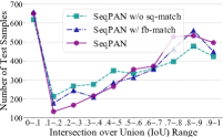
(a) Charades-STA

(b) ActivityNet Captions

Figure 7: Plots of the number of predicted test samples within different IoU ranges on Charades-STA and ANetCaps.

4.3 Discussion and Analysis

We perform in-depth ablation studies to analyze the effectiveness of the SeqPAN. We run all the experiments 5 times and report 5-run average.

Analysis on Self-Guided Parallel Attention. The SGPA (see Figure 4) is a variant of transformer (TRM), designed for learning cross-modality interactions between visual and text features. Here, we compare SGPA with standard TRMs. To better reflect the performance of different TRMs, we remove the sequence matching component and only use a single block (i.e., $N_{\text{SGPA}}=1$) in this experiment. The results are reported in Table 4. Observe that SGPA is superior to TRMs on both datasets. Co-TRM performs better on Charades-STA but worse on ANetCaps comparing with Se-TRM. Compared to Se-TRM and Co-TRM, SGPA learns both self-modal contexts and cross-modal interactions, which is approximately equivalent to parallel connection of two modules.

Impact of SGPA block numbers $N_{\text{SGPA}}$. We now study the impact of SGPA block numbers on Charades-STA and ANetCaps. We evaluate five different values of $N_{\text{SGPA}}$ from $1$ to $5$. The performance across the number of SGPA blocks in SeqPAN are plotted in Figures 5(a) and 5(b). Best performance is achieved at $N_{\text{SGPA}}=2$ on both datasets. In general, along with increasing $N_{\text{SGPA}}$, the performance of SeqPAN first increases and then gradually decreases, on both datasets. We also note that performance on Charades-STA is not very sensitive to the setting of $N_{\text{SGPA}}$.

Analysis on Sequence Matching. The conventional matching strategy Yuan et al. (2019b); Lu et al. (2019a); Mun et al. (2020) (denoted by fb-match) is to predict whether a frame is inside or outside of target moment, i.e., foreground or background. In SeqPAN, we predict begin-, inside- and end-regions, and introduce label embeddings ($\bm{E}_{\text{lab}}$) to represent each region. The prediction process also uses the Gumbel-Max trick. In this experiment, we analyze the effects of label embeddings and Gumbel-Max trick in sequence matching.

Summarized in Table 5, both Gumbel-Max trick (denoted by $G$) and label embeddings contribute to the grounding performance improvement. In addition, consistent improvements are observed by incorporating $G$ and $\bm{E}_{\text{lab}}$ into the model. SeqPAN is superior to SeqPAN w/ fb-match over all evaluation metrics. The performance improvements are more significant under more strict metrics. The results show that sq-match is more effective than the fb-match strategy. Regional indication of potential positions of start/end boundaries does help the model to produce accurate predictions.

Impact of Annealing Temperature $\tau$. We then analyze the impact of annealing temperature $\tau$ of Gumbel-Softmax in sequence matching module. Gumbel-Softmax distributions are identical to a categorical distribution when $\tau\to 0^{+}$. With $\tau\to\infty$, its distribution is smooth. We evaluate 11 different $\tau$ values from $0.01$ to $1.0$, where $0.01$ is used to approximate $0.0$ since $0.0$ is not divisible. The results are compared against vanilla Softmax as a baseline. For vanilla Softmax, we multiply the probability distribution of labels with $\bm{E}_{\text{lab}}$, to aggregate label information into the visual representations.

Figure 6 plots the results of different $\tau$’s on Charades-STA and ANetCaps, respectively. We observe similar patterns on the four sets of results. The best performance is achieved when $\tau=0.3$ over both metrics on both datasets. From Figure 6(a), when $\tau$ is too small or too large (i.e., the probability distribution from Gumbel-Softmax becomes too sharp or too smooth), Gumbel-Softmax performs poorer than vanilla Softmax. This result suggests that a proper annealing temperature $\tau$ is crucial to achieve good performance. Similar observations hold on ANetCaps (see Figure 6(b)).

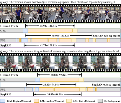
Figure 8: Qualitative results of SeqPAN and SeqPAN w/o sq-match on ANetCaps. “GSL” is the ground truth sequence labels; “PSL” is the predicted labels by sq-match of SeqPAN.

4.4 Qualitative Analysis

Figure 7 shows the number of predicted test samples within different IoU ranges on Charades-STA and ANetCaps. Here, we compare SeqPAN with two of its variants: (i) removal of sequence matching module, and (ii) replacement of sequence matching with fb-match. All three variants show similar patterns. Nevertheless, within the higher IoU ranges, e.g., $\text{IoU}\geq 0.5$ on both datasets, SeqPAN and the variant with fb-match outperform the variant without sequence matching. The results show that having auxiliary objectives (e.g., foreground/background or sequential regions) is helpful in video grounding task. Results in Figure 7 also show that our sequence matching is more effective than fb-match, for highlighting the correction regions for predicting start/end boundaries.

Figure 8 depicts two video grounding examples from the ANetCaps dataset. From the two examples, the moments retrieved by SeqPAN are closer to the ground truth than that are retrieved by SeqPAN without utilizing the sq-match strategy. Besides, the start and end boundaries predicted by SeqPAN are roughly constrained within the pre-set potential start and end regions. In addition, the predicted sequence labels (PSL) in Figure 8 also reveal the weakness of sq-match strategy. The predicted labels by sq-match strategy are not continuous, where multiple start, inside, and end regions are generated. In consequence, the localizer may be affected by wrongly predicted regions and leads to inaccurate results. To further constrain the generated regions is part of our future work.

5 Conclusion

In this work, we propose a Parallel Attention Network with Sequence matching (SeqPAN) to address the language query-based video grounding problem. We design a parallel attention module to improve the multimodal representation learning by capturing both self- and cross-modal attentive information simultaneously. In addition, we propose a sequence matching strategy, which explicitly indicates the potential start and end regions of the target moment to allow the localizer precisely predicting the boundaries. Through extensive experimental studies, we show that SeqPAN outperforms the state-of-the-art methods on three benchmark datasets; and both the proposed parallel attention and sequence matching modules contribute to the grounding performance improvement.

This appendix contains two sections. Section A provides (A.1) a detailed comparison between the proposed SGPA and standard transformer blocks, (A.2) technical details of the video-query integration module, and (A.3) categorical reparameterization used in the sequence matching module. Section B describes statistics on the benchmark datasets and parameter settings in our experiments.

Appendix A Additional Comparison and Technical Details

A.1 SGPA versus Standard Transformers

Two ways are mainly used to adopt the transformer block for multi-modal representation learning:

• Transformer block with the self-attention (Se-TRM), which encodes visual and textual inputs in separate streams, shown in Figure 9(a).

• Transformer block with the cross-attention (Co-TRM), which encodes both visual and textual inputs with interactions through co-attention, shown in Figure 9(b).

Several works Lu et al. (2019a); Chen et al. (2020a); Zhang et al. (2020a) adopt Se-TRM to learn visual and textual representations in video grounding task. Se-TRM separately encodes each modality, it focuses on learning the refined unimodal representations within each modality for video and text respectively. Without any connection between two modalities, Se-TRM cannot use information from other modality to improve the representations.

Co-TRM is commonly used as a basic component in various vision-language methods Tan and Bansal (2019); Lu et al. (2019b); Lei et al. (2020). Co-TRM relies on co-attention to learn the cross-modal representations for both visual and textual inputs. However, Co-TRM lacks the ability to encode self-attentive context within each modality.

The cascade of Se-TRM and Co-TRM is also used in recent vision-language models Tan and Bansal (2019); Lu et al. (2019b); Zhu and Yang (2020); Lei et al. (2020) to learn both unimodal and cross-modal representations. In general, there are two cascade forms: 1) stacking Co-TRM upon Se-TRM (SeCo-TRM) in Figure 10(a); and 2) stacking Se-TRM upon Co-TRM (CoSe-TRM) in Figure 10(b). These stacked TRMs learn the unimodal and cross-modal information in a sequence manner. Hence, their final outputs focus more on either the self-attentive contexts or cross-modal interactions. Our SGPA combines advantages of both Se-TRM and Co-TRM, but not through cascade. As shown in Figure 9(c), SGPA contains two parallel multi-head attention blocks. One block takes single modality as input and the other takes both modalities as inputs. Thus, SGPA is able to learn both unimodal and cross-modal representations simultaneously. Then, a cross-gating strategy is designed to fuse the self- and cross-attentive representations. We also employ a self-guided head to replace the feed forward layer in transformer block. This design implicitly emphasizes informative representations by measuring the confidence of each element.

Table 6 reports the performance of SGPA and standard TRMs on Charades-STA and ANetCaps datasets. Here, we regard both SeCo-TRM and CoSe-TRM as single block. The results show that both PA (a SGPA variant without self-guided head) and SGPA are superior to standard TRMs.

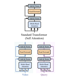
(a) Transformer Block (Self Attn)

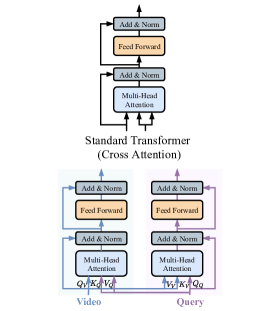
(b) Transformer Block (Cross Attn)

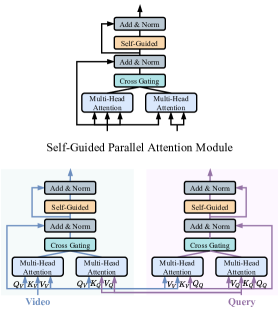
(c) Self Guided Parallel Attention (Ours)

Figure 9: The structures of standard transformer blocks and self-guided parallel attention module. Top: the structure of each module; Bottom: the parallel streams of encoding visual and textual inputs. (a) The standard transformer block with self-attention; (b) The standard transformer block with cross-attention; (c) The self-guided parallel attention (SGPA) module.

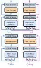
(a) SeCo-TRM Block

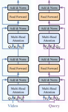
(b) CoSe-TRM Block

Figure 10: The structures of SeCo-TRM and CoSe-TRM.

Methods	$\text{R@}1,\text{IoU}=\mu$
	$\mu=0.3$	$\mu=0.5$	$\mu=0.7$
Charades-STA
Se-TRM	68.84 (0.46)	51.92 (0.54)	34.58 (0.18)
Co-TRM	69.03 (0.49)	52.34 (0.50)	35.07 (0.32)
SeCo-TRM	69.11 (0.24)	52.63 (0.49)	35.17 (0.22)
CoSe-TRM	69.08 (0.26)	52.82 (0.43)	35.09 (0.50)
PA	69.21 (0.27)	54.37 (0.46)	36.22 (0.49)
SGPA	69.47 (0.32)	54.63 (0.43)	36.36 (0.24)
ActivityNet Captions
Se-TRM	57.64 (0.38)	40.76 (0.35)	25.10 (0.30)
Co-TRM	57.39 (0.29)	40.55 (0.45)	24.85 (0.47)
SeCo-TRM	57.47 (0.38)	40.70 (0.24)	25.07 (0.21)
CoSe-TRM	57.72 (0.41)	40.85 (0.17)	25.16 (0.15)
PA	58.27 (0.13)	41.59 (0.24)	25.88 (0.28)
SGPA	58.40 (0.31)	41.72 (0.19)	26.07 (0.16)

Table 6: Comparison between SGPA with standard transformer blocks on Charades-STA and ANetCaps, where PA is the SGPA without self-guided head (i.e., replaced by FFN) The scores in bracket denotes standard deviation.

A.2 Video-Query Integration Computation

This section presents the detailed computation process of video-query integration (see Section 3.1.3).

Given two inputs $\bm{X}\in\mathbb{R}^{d\times N_{x}}$ and $\bm{Y}\in\mathbb{R}^{d\times N_{y}}$, the context-query attention first computes similarities between each pair of $\bm{X}$ and $\bm{Y}$ elements as:

$$\mathcal{S}=\bm{X}^{\top}\cdot\bm{W}\cdot\bm{Y}$$ (16)

where $\bm{W}\in\mathbb{R}^{d\times d}$ and $\mathcal{S}\in\mathbb{R}^{N_{x}\times N_{y}}$. Then $X$-to-$Y$ and $Y$-to-$X$ attention weights are computed by:

$$\mathcal{A}_{\text{XY}} =\mathcal{S}_{r}\cdot\bm{Y}^{\top}\in\mathbb{R}^{N_{x}\times d}$$ (17)

$$\mathcal{A}_{\text{YX}} =\mathcal{S}_{r}\cdot\mathcal{S}^{\top}_{c}\cdot\bm{X}^{\top}\in\mathbb{R}^{N_{x}\times d}$$

where $\mathcal{S}_{r}$ and $\mathcal{S}_{c}$ are the row- and column-wise normalization of $\mathcal{S}$ by Softmax function. The final output of context-query attention is calculated as:

$$\bm{X}^{Y}=\mathtt{FFN}\big{(}[\bm{X};\mathcal{A}_{\text{XY}}^{\top};\bm{X}\odot\mathcal{A}_{\text{XY}}^{\top};\bm{X}\odot\mathcal{A}_{\text{YX}}^{\top}]\big{)}$$ (18)

where $\odot$ denotes element-wise multiplication, “;” represents concatenation operation, and $\bm{X}^{Y}\in\mathbb{R}^{d\times N_{x}}$. In this way, the information of $\bm{Y}$ is properly fused into $\bm{X}$.

By setting $\bm{X}=\bm{\bar{V}}\in\mathbb{R}^{d\times N}$ and $\bm{Y}=\bm{\bar{Q}}\in\mathbb{R}^{d\times M}$, we can derive the query-aware video representations $\bm{V}^{Q}\in\mathbb{R}^{d\times N}$. Similarly, the video-aware query representations $\bm{Q}^{V}\in\mathbb{R}^{d\times M}$ is obtained by setting $\bm{X}=\bm{\bar{Q}}$ and $\bm{Y}=\bm{\bar{V}}$.

Next, we encode $\bm{Q}^{V}=[\bm{q}_{0}^{V},\dots,\bm{q}_{M-1}^{V}]$ into sentence representation $\bm{q}$ with additive attention:

$$\bm{\alpha} =\mathtt{Softmax}\big{(}\bm{W}_{\alpha}\cdot\bm{Q}^{V})\big{)}\in\mathbb{R}^{M}$$ (19)

$$\bm{q} =\sum_{i=0}^{M-1}\alpha_{i}\times\bm{q}_{i}^{V}\in\mathbb{R}^{d}$$

where $\bm{W}_{\alpha}\in\mathbb{R}^{1\times d}$. The $\bm{q}$ is then concatenated with each element of $\bm{V}^{Q}$ as $\bm{H}=[\bm{h}_{1},\dots,\bm{h}_{n}]\in\mathbb{R}^{2d\times N}$, where $\bm{h}_{i}=[\bm{v}_{i}^{Q};\bm{q}]$. Finally, the query-attended visual representation is computed as

$$\bm{\bar{H}}=\bm{W}_{h}\cdot\bm{H}+\bm{b}_{h}$$ (20)

where $W_{h}\in\mathbb{R}^{d\times 2d}$ and $b_{h}\in\mathbb{R}^{d}$ denote the learnable weight and bias, and $\bm{\bar{H}}\in\mathbb{R}^{d\times N}$.

Dataset	Domain	$N_{\text{V}}$ (train/val/test)	$N_{\text{A}}$ (train/val/test)	$\bar{N}_{\text{A/V}}$	$N_{\text{Vocab}}$	$\bar{L}_{V}$ (s)	$\bar{L}_{Q}$	$\bar{L}_{M}$ (s)
Charades-STA	Indoors	$5,338/\text{-}/1,334$	$12,408/\text{-}/3,720$	$2.42$	$1,303$	$30.59$	$7.22$	$8.22$
ActivityNet Captions	Open	$10,009/\text{-}/4,917$	$37,421/\text{-}/17,505$	$3.68$	$12,460$	$117.61$	$14.78$	$36.18$
TACoS Gao et al. (2017)	Cook	$75/27/25$	$10,146/4,589/4,083$	$148.17$	$2,033$	$287.14$	$10.05$	$5.45$
TACoS Zhang et al. (2020b)			$9,790/4,436/4,001$	$143.52$	$1,983$	$287.14$	$9.42$	$25.26$

Table 7: Statistics of the evaluated video grounding benchmark datasets, where $N_{\text{V}}$ is number of videos, $N_{\text{A}}$ is number of annotations, $\bar{N}_{\text{A/V}}$ denotes the average number of annotations per video, $N_{\textrm{Vocab}}$ is the vocabulary size of lowercase words, $\bar{L}_{V}$ denotes the average length of videos in seconds, $\bar{L}_{Q}$ denotes the average number of words in the sentence queries and $\bar{L}_{M}$ represents the average length of temporal moments in seconds.

A.3 Categorical Reparameterization

This section provides a brief introduction of the categorical reparameterization strategy used in sequence matching module (see Section 3.1.4).

Categorical reparameterization, e.g., reinforce-based approaches Sutton et al. (2000); Schulman et al. (2015), straight-through estimators Bengio et al. (2013) and Gumbel-Softmax Jang et al. (2017); Maddison et al. (2017), is a strategy that enables discrete categorical variables to back-propagate in neural networks. It aims to estimate smooth gradient with a continuous relaxation for categorical variable. In this work, we use Gumbel-Softmax to approximate the sequence labels from a probability distribution. Then those labels are applied to lookup the corresponding embeddings for region representation in the sequence matching module of SeqPAN.

Let $\bm{x}=(x_{1},\dots,x_{l})$ be a categorical distribution, where $l$ is the number of categories, $x_{c}$ is the probability score of category $c$ and $\sum_{c=1}^{l}x_{c}=1$. Given the i.i.d. Gumbel noise $\bm{g}=(g_{1},\dots,g_{l})$ from $\mathtt{Gumbel}(0,1)$ distribution, the soft categorical sample can be computed as:

$$\bm{y}=\mathtt{Softmax}\big{(}(\log(\bm{x})+\bm{g})/\tau\big{)}$$ (21)

where $\tau>0$ is annealing temperature, and Eq. 21 is referred as Gumbel-Softmax operation on $\bm{x}$. As $\tau\to 0^{+}$, $\bm{y}$ is equivalent to the Gumbel-Max form Gumbel (1954); Maddison et al. (2014) as:

$$\bm{\hat{y}}=\mathtt{Onehot}\big{(}\arg\max(\log(\bm{x})+\bm{g})\big{)}$$ (22)

where $\bm{\hat{y}}$ is an unbiased sample from $\bm{x}$ and thus we can draw differentiable samples from the distribution during training. Note, when input $\bm{x}$ is unnormalized, the $\log(\cdot)$ operator in Eq. 21 and 22 shall be omitted Jang et al. (2017); Dong and Yang (2019). During inference, discrete samples can be drawn with the Gumbel-Max trick directly.

Appendix B Dataset and Parameter Settings

B.1 Dataset Statistics

The statistics of the evaluated benchmark datasets are summarized in Table 7. Charades-STA dataset consists of $6,672$ videos and $16,128$ annotations (i.e., moment-query pairs) in total. ActivityNet Captions (ANetCaps) dataset is taken from the ActivityNet Heilbron et al. (2015). The average duration is about $120$ seconds and each video contains $3.68$ annotations on average. TACoS dataset contains $127$ cooking activities videos with average duration of $4.79$ minutes, and $18,818$ annotations in total. We follow the same train/val/test split as Gao et al. (2017). Besides, Zhang et al. (2020b) pre-processes the TACoS dataset, hence their version is slightly different from the original version. Detailed statistics are summarized in Table 7.

B.2 Hyper-Parameter Settings

We follow Ghosh et al. (2019); Mun et al. (2020); Rodriguez et al. (2020); Zhang et al. (2020a) and use 3D ConvNet pre-trained on Kinetics dataset (i.e., I3D) Carreira and Zisserman (2017) to extract visual features from videos. The maximal visual feature sequence lengths are set to $64$, $100$, and $256$ for Charades-STA, ActivityNet Captions, and TACoS, respectively. This setting is based on the average video lengths in the three datasets. The feature sequence length of a video will be uniformly downsampled if it is larger than the pre-set threshold, or zero-padding otherwise. For the language queries, we lowercase all the words and initialize them with GloVe Pennington et al. (2014) embeddings. The word embeddings and extracted visual features are fixed during training.

For other hyper-parameters, we use the same settings for all datasets. The dimension of the hidden layers is $128$; the head number in multi-head attention is $8$; the number of SGPA blocks ($N_{\text{SGPA}}$) is $2$; the annealing temperature $\tau$ of Gumbel-Softmax is $0.3$; The Dropout Srivastava et al. (2014) is $0.2$. The maximal training epochs $E=100$ is used, with batch size of $16$ and early stopping tolerance of $10$ epochs. We adopt Adam Kingma and Ba (2015) optimizer, with initial learning rate of $\beta_{0}=0.0001$, weight decay $0.01$, and gradient clipping $1.0$, to train the model. The learning rate decay strategy is defined as $\beta_{e}=\beta_{0}\times(1-\frac{e}{E})$, where $e$ denotes the $e$-th training epoch.

The SeqPAN is implemented using TensorFlow 1.15.0 with CUDA 10.0 and cudnn 7.6.5. All the experiments are conducted on a workstation with dual NVIDIA GeForce RTX 2080Ti GPUs.

References

- Bahdanau et al. (2015) Dzmitry Bahdanau, Kyunghyun Cho, and Yoshua Bengio. 2015. Neural machine translation by jointly learning to align and translate. In International Conference on Learning Representations.
- Bengio et al. (2013) Yoshua Bengio, N. Léonard, and Aaron C. Courville. 2013. Estimating or propagating gradients through stochastic neurons for conditional computation. ArXiv, abs/1308.3432.
- Brock et al. (2019) Andrew Brock, Jeff Donahue, and Karen Simonyan. 2019. Large scale GAN training for high fidelity natural image synthesis. In International Conference on Learning Representations.
- Cao et al. (2020) Da Cao, Yawen Zeng, Meng Liu, Xiangnan He, Meng Wang, and Zheng Qin. 2020. Strong: Spatio-temporal reinforcement learning for cross-modal video moment localization. In Proceedings of the 28th ACM International Conference on Multimedia.
- Carreira and Zisserman (2017) João Carreira and Andrew Zisserman. 2017. Quo vadis, action recognition? a new model and the kinetics dataset. In IEEE Conference on Computer Vision and Pattern Recognition, pages 4724–4733.
- Chen et al. (2018) Jingyuan Chen, Xinpeng Chen, Lin Ma, Zequn Jie, and Tat-Seng Chua. 2018. Temporally grounding natural sentence in video. In Proceedings of the 2018 Conference on Empirical Methods in Natural Language Processing, pages 162–171.
- Chen et al. (2019) Jingyuan Chen, Lin Ma, Xinpeng Chen, Zequn Jie, and Jiebo Luo. 2019. Localizing natural language in videos. In Proceedings of the AAAI Conference on Artificial Intelligence, volume 33, pages 8175–8182.
- Chen et al. (2020a) Long Chen, Chujie Lu, Siliang Tang, Jun Xiao, Dong Zhang, Chilie Tan, and Xiaolin Li. 2020a. Rethinking the bottom-up framework for query-based video localization. In Proceedings of the AAAI Conference on Artificial Intelligence.
- Chen et al. (2020b) Shaoxiang Chen, Wenhao Jiang, Wei Liu, and Yu-Gang Jiang. 2020b. Learning modality interaction for temporal sentence localization and event captioning in videos. In The European Conference on Computer Vision.
- Chen and Jiang (2019) Shaoxiang Chen and Yu-Gang Jiang. 2019. Semantic proposal for activity localization in videos via sentence query. In Proceedings of the AAAI Conference on Artificial Intelligence, volume 33.
- Dong and Yang (2019) Xuanyi Dong and Yi Yang. 2019. Searching for a robust neural architecture in four gpu hours. In Proceedings of the IEEE Conference on computer vision and pattern recognition, pages 1761–1770.
- Feichtenhofer et al. (2019) Christoph Feichtenhofer, Haoqi Fan, Jitendra Malik, and Kaiming He. 2019. Slowfast networks for video recognition. In Proceedings of the IEEE international conference on computer vision.
- Gao et al. (2017) Jiyang Gao, Chen Sun, Zhenheng Yang, and Ramakant Nevatia. 2017. Tall: Temporal activity localization via language query. In IEEE International Conference on Computer Vision, pages 5277–5285.
- Ge et al. (2019) Runzhou Ge, Jiyang Gao, Kan Chen, and Ram Nevatia. 2019. Mac: Mining activity concepts for language-based temporal localization. In IEEE Winter Conference on Applications of Computer Vision.
- Ghosh et al. (2019) Soham Ghosh, Anuva Agarwal, Zarana Parekh, and Alexander Hauptmann. 2019. ExCL: Extractive Clip Localization Using Natural Language Descriptions. In Proceedings of the 2019 Conference of the North American Chapter of the Association for Computational Linguistics, pages 1984–1990.
- Gumbel (1954) Emil Julius Gumbel. 1954. Statistical theory of extreme values and some practical applications: a series of lectures, volume 33. US Government Printing Office.
- Hahn et al. (2020) Meera Hahn, Asim Kadav, James M Rehg, and Hans Peter Graf. 2020. Tripping through time: Efficient localization of activities in videos. In The British Machine Vision Conference.
- He et al. (2019) Dongliang He, Xiang Zhao, Jizhou Huang, Fu Li, Xiao Liu, and Shilei Wen. 2019. Read, watch, and move: Reinforcement learning for temporally grounding natural language descriptions in videos. In Proceedings of the AAAI Conference on Artificial Intelligence, volume 33, pages 8393–8400.
- Heilbron et al. (2015) F. C. Heilbron, V. Escorcia, B. Ghanem, and J. C. Niebles. 2015. Activitynet: A large-scale video benchmark for human activity understanding. In IEEE Conference on Computer Vision and Pattern Recognition, pages 961–970.
- Hendricks et al. (2018) Lisa Anne Hendricks, Oliver Wang, Eli Shechtman, Josef Sivic, Trevor Darrell, and Bryan Russell. 2018. Localizing moments in video with temporal language. In Proceedings of the 2018 Conference on Empirical Methods in Natural Language Processing.
- Hendricks et al. (2017) Lisa Anne Hendricks, Oliver Wang, Eli Shechtman, Josef Sivic, Trevor Darrell, and Bryan C. Russell. 2017. Localizing moments in video with natural language. In 2017 IEEE International Conference on Computer Vision, pages 5804–5813.
- Hu et al. (2019) Ronghang Hu, Daniel Fried, Anna Rohrbach, Dan Klein, Trevor Darrell, and Kate Saenko. 2019. Are you looking? grounding to multiple modalities in vision-and-language navigation. In Proceedings of the 57th Annual Meeting of the Association for Computational Linguistics, pages 6551–6557.
- Huang et al. (2018) Hsin-Yuan Huang, Chenguang Zhu, Yelong Shen, and Weizhu Chen. 2018. Fusionnet: Fusing via fully-aware attention with application to machine comprehension. In International Conference on Learning Representations.
- Jang et al. (2017) Eric Jang, Shixiang Gu, and Ben Poole. 2017. Categorical reparameterization with gumbel-softmax. In International Conference on Learning Representations.
- Kingma and Ba (2015) Diederik P. Kingma and Jimmy Ba. 2015. Adam: A method for stochastic optimization. In International Conference on Learning Representations.
- Krishna et al. (2017) R. Krishna, K. Hata, F. Ren, L. Fei-Fei, and J. C. Niebles. 2017. Dense-captioning events in videos. In IEEE International Conference on Computer Vision, pages 706–715.
- Lample et al. (2016) Guillaume Lample, Miguel Ballesteros, Sandeep Subramanian, Kazuya Kawakami, and Chris Dyer. 2016. Neural architectures for named entity recognition. In Proceedings of the 2016 Conference of the North American Chapter of the Association for Computational Linguistics.
- Lei et al. (2020) Jie Lei, Licheng Yu, Tamara L Berg, and Mohit Bansal. 2020. Tvr: A large-scale dataset for video-subtitle moment retrieval. In The European Conference on Computer Vision.
- Li et al. (2020) Linjie Li, Yen-Chun Chen, Yu Cheng, Zhe Gan, Licheng Yu, and Jingjing Liu. 2020. HERO: Hierarchical encoder for Video+Language omni-representation pre-training. In Proceedings of the 2020 Conference on Empirical Methods in Natural Language Processing, pages 2046–2065.
- Lin et al. (2018) Tianwei Lin, Xu Zhao, Haisheng Su, Chongjing Wang, and Ming Yang. 2018. Bsn: Boundary sensitive network for temporal action proposal generation. In Proceedings of the European Conference on Computer Vision, pages 3–19.
- Lin et al. (2020) Zhijie Lin, Zhou Zhao, Zhu Zhang, Qi Wang, and Huasheng Liu. 2020. Weakly-supervised video moment retrieval via semantic completion network. In Proceedings of the AAAI Conference on Artificial Intelligence.
- Liu et al. (2018a) Bingbin Liu, Serena Yeung, Edward Chou, De-An Huang, Li Fei-Fei, and Juan Carlos Niebles. 2018a. Temporal modular networks for retrieving complex compositional activities in videos. In The European Conference on Computer Vision.
- Liu et al. (2020) Daizong Liu, Xiaoye Qu, Xiao-Yang Liu, Jianfeng Dong, Pan Zhou, and Zichuan Xu. 2020. Jointly cross-and self-modal graph attention network for query-based moment localization. In Proceedings of the 28th ACM International Conference on Multimedia, pages 4070–4078.
- Liu et al. (2018b) Meng Liu, Xiang Wang, Liqiang Nie, Qi Tian, Baoquan Chen, and Tat-Seng Chua. 2018b. Cross-modal moment localization in videos. In Proceedings of the 26th ACM International Conference on Multimedia, pages 843–851.
- Lu et al. (2019a) Chujie Lu, Long Chen, Chilie Tan, Xiaolin Li, and Jun Xiao. 2019a. DEBUG: A dense bottom-up grounding approach for natural language video localization. In Proceedings of the 2019 Conference on Empirical Methods in Natural Language Processing and the 9th International Joint Conference on Natural Language Processing, pages 5147–5156.
- Lu et al. (2019b) Jiasen Lu, Dhruv Batra, Devi Parikh, and Stefan Lee. 2019b. Vilbert: Pretraining task-agnostic visiolinguistic representations for vision-and-language tasks. In Advances in Neural Information Processing Systems, pages 13–23.
- Ma and Hovy (2016) Xuezhe Ma and Eduard Hovy. 2016. End-to-end sequence labeling via bi-directional lstm-cnns-crf. In Proceedings of the 54th Annual Meeting of the Association for Computational Linguistics.
- Maddison et al. (2017) Chris J. Maddison, Andriy Mnih, and Yee Whye Teh. 2017. The concrete distribution: A continuous relaxation of discrete random variables. In International Conference on Learning Representations.
- Maddison et al. (2014) Chris J Maddison, Daniel Tarlow, and Tom Minka. 2014. A* sampling. In Advances in Neural Information Processing Systems, pages 3086–3094.
- Mithun et al. (2019) Niluthpol Chowdhury Mithun, Sujoy Paul, and Amit K. Roy-Chowdhury. 2019. Weakly supervised video moment retrieval from text queries. In Computer Vision and Pattern Recognition, pages 11592–11601.
- Mun et al. (2020) Jonghwan Mun, Minsu Cho, and Bohyung Han. 2020. Local-global video-text interactions for temporal grounding. In Proceedings of the IEEE/CVF Conference on Computer Vision and Pattern Recognition.
- Pennington et al. (2014) Jeffrey Pennington, Richard Socher, and Christopher Manning. 2014. Glove: Global vectors for word representation. In Proceedings of the 2014 Conference on Empirical Methods in Natural Language Processing, pages 1532–1543.
- Regneri et al. (2013) Michaela Regneri, Marcus Rohrbach, Dominikus Wetzel, Stefan Thater, Bernt Schiele, and Manfred Pinkal. 2013. Grounding action descriptions in videos. TACL, 1:25–36.
- Rodriguez et al. (2020) Cristian Rodriguez, Edison Marrese-Taylor, Fatemeh Sadat Saleh, Hongdong Li, and Stephen Gould. 2020. Proposal-free temporal moment localization of a natural-language query in video using guided attention. In The IEEE Winter Conference on Applications of Computer Vision.
- Rohrbach et al. (2012) Marcus Rohrbach, Michaela Regneri, Mykhaylo Andriluka, Sikandar Amin, Manfred Pinkal, and Bernt Schiele. 2012. Script data for attribute-based recognition of composite activities. In The European Conference on Computer Vision.
- Schulman et al. (2015) John Schulman, Nicolas Heess, Theophane Weber, and Pieter Abbeel. 2015. Gradient estimation using stochastic computation graphs. In Advances in Neural Information Processing Systems, pages 3528–3536.
- Seo et al. (2017) Minjoon Seo, Aniruddha Kembhavi, Ali Farhadi, and Hannaneh Hajishirzi. 2017. Bidirectional attention flow for machine comprehension. In International Conference on Learning Representations.
- Shao et al. (2018) Dian Shao, Yu Xiong, Yue Zhao, Qingqiu Huang, Yu Qiao, and Dahua Lin. 2018. Find and focus: Retrieve and localize video events with natural language queries. In The European Conference on Computer Vision.
- Shou et al. (2016) Zheng Shou, Dongang Wang, and Shih-Fu Chang. 2016. Temporal action localization in untrimmed videos via multi-stage cnns. In Proceedings of the IEEE Conference on Computer Vision and Pattern Recognition, pages 1049–1058.
- Sigurdsson et al. (2016) Gunnar A. Sigurdsson, Gül Varol, Xiaolong Wang, Ali Farhadi, Ivan Laptev, and Abhinav Gupta. 2016. Hollywood in homes: Crowdsourcing data collection for activity understanding. In European Conference on Computer Vision, pages 510–526.
- Srivastava et al. (2014) Nitish Srivastava, Geoffrey Hinton, Alex Krizhevsky, Ilya Sutskever, and Ruslan Salakhutdinov. 2014. Dropout: A simple way to prevent neural networks from overfitting. Journal of Machine Learning Research, 15(56):1929–1958.
- Su et al. (2020) Weijie Su, Xizhou Zhu, Yue Cao, Bin Li, Lewei Lu, Furu Wei, and Jifeng Dai. 2020. Vl-bert: Pre-training of generic visual-linguistic representations. In International Conference on Learning Representations.
- Sutton et al. (2000) Richard S Sutton, David A McAllester, Satinder P Singh, and Yishay Mansour. 2000. Policy gradient methods for reinforcement learning with function approximation. In Advances in neural information processing systems, pages 1057–1063.
- Tan and Bansal (2019) Hao Tan and Mohit Bansal. 2019. LXMERT: Learning cross-modality encoder representations from transformers. In Proceedings of the Conference on Empirical Methods in Natural Language Processing.
- Tran et al. (2015) Du Tran, Lubomir Bourdev, Rob Fergus, Lorenzo Torresani, and Manohar Paluri. 2015. Learning spatiotemporal features with 3d convolutional networks. In Proceedings of the IEEE international conference on computer vision, pages 4489–4497.
- Vaswani et al. (2017) Ashish Vaswani, Noam Shazeer, Niki Parmar, Jakob Uszkoreit, Llion Jones, Aidan N Gomez, Ł ukasz Kaiser, and Illia Polosukhin. 2017. Attention is all you need. In Advances in Neural Information Processing Systems, pages 5998–6008.
- Wang et al. (2020a) Hao Wang, Zheng-Jun Zha, Xuejin Chen, Zhiwei Xiong, and Jiebo Luo. 2020a. Dual path interaction network for video moment localization. In Proceedings of the 28th ACM International Conference on Multimedia, MM ’20, page 4116–4124.
- Wang et al. (2020b) Jingwen Wang, Lin Ma, and Wenhao Jiang. 2020b. Temporally grounding language queries in videos by contextual boundary-aware prediction. In AAAI.
- Wang et al. (2019) Weining Wang, Yan Huang, and Liang Wang. 2019. Language-driven temporal activity localization: A semantic matching reinforcement learning model. In Proceedings of the IEEE Conference on Computer Vision and Pattern Recognition.
- Wu et al. (2020a) Jie Wu, Guanbin Li, Xiaoguang Han, and Liang Lin. 2020a. Reinforcement learning for weakly supervised temporal grounding of natural language in untrimmed videos. In Proceedings of the 28th ACM International Conference on Multimedia.
- Wu et al. (2020b) Jie Wu, Guanbin Li, Si Liu, and Liang Lin. 2020b. Tree-structured policy based progressive reinforcement learning for temporally language grounding in video. In Proceedings of the AAAI Conference on Artificial Intelligence.
- Xu et al. (2019) Huijuan Xu, Kun He, Bryan A. Plummer, L. Sigal, Stan Sclaroff, and Kate Saenko. 2019. Multilevel language and vision integration for text-to-clip retrieval. In Proceedings of the AAAI Conference on Artificial Intelligence, volume 33, pages 9062–9069.
- Yang et al. (2019) Zhilin Yang, Zihang Dai, Yiming Yang, Jaime Carbonell, Russ R Salakhutdinov, and Quoc V Le. 2019. Xlnet: Generalized autoregressive pretraining for language understanding. In Advances in Neural Information Processing Systems, pages 5754–5764.
- Yu et al. (2018) Adams Wei Yu, David Dohan, Quoc Le, Thang Luong, Rui Zhao, and Kai Chen. 2018. Fast and accurate reading comprehension by combining self-attention and convolution. In International Conference on Learning Representations.
- Yu et al. (2019) Zhou Yu, Dejing Xu, Jun Yu, Ting Yu, Zhou Zhao, Yueting Zhuang, and Dacheng Tao. 2019. Activitynet-qa: A dataset for understanding complex web videos via question answering. In Proceedings of the AAAI Conference on Artificial Intelligence.
- Yuan et al. (2019a) Yitian Yuan, Lin Ma, Jingwen Wang, Wei Liu, and Wenwu Zhu. 2019a. Semantic conditioned dynamic modulation for temporal sentence grounding in videos. In Advances in Neural Information Processing Systems, pages 536–546.
- Yuan et al. (2019b) Yitian Yuan, Tao Mei, and Wenwu Zhu. 2019b. To find where you talk: Temporal sentence localization in video with attention based location regression. In AAAI, volume 33, pages 9159–9166.
- Zeng et al. (2020) Runhao Zeng, Haoming Xu, Wenbing Huang, Peihao Chen, Mingkui Tan, and Chuang Gan. 2020. Dense regression network for video grounding. In Proceedings of the IEEE/CVF Conference on Computer Vision and Pattern Recognition, pages 10287–10296.
- Zhang et al. (2019a) Da Zhang, Xiyang Dai, Xin Wang, Yuan-Fang Wang, and Larry S Davis. 2019a. Man: Moment alignment network for natural language moment retrieval via iterative graph adjustment. In Proceedings of the IEEE Conference on Computer Vision and Pattern Recognition, pages 1247–1257.
- Zhang et al. (2021) Hao Zhang, Aixin Sun, Wei Jing, Liangli Zhen, Joey Tianyi Zhou, and Rick Siow Mong Goh. 2021. Natural language video localization: A revisit in span-based question answering framework. IEEE Transactions on Pattern Analysis and Machine Intelligence.
- Zhang et al. (2020a) Hao Zhang, Aixin Sun, Wei Jing, and Joey Tianyi Zhou. 2020a. Span-based localizing network for natural language video localization. In Proceedings of the 58th Annual Meeting of the Association for Computational Linguistics, pages 6543–6554.
- Zhang et al. (2020b) Songyang Zhang, Houwen Peng, Jianlong Fu, and Jiebo Luo. 2020b. Learning 2d temporal adjacent networks formoment localization with natural language. In Proceedings of the AAAI Conference on Artificial Intelligence.
- Zhang et al. (2019b) Songyang Zhang, Jinsong Su, and Jiebo Luo. 2019b. Exploiting temporal relationships in video moment localization with natural language. In Proceedings of ACM International Conference on Multimedia.
- Zhang et al. (2019c) Zhu Zhang, Zhijie Lin, Zhou Zhao, and Zhenxin Xiao. 2019c. Cross-modal interaction networks for query-based moment retrieval in videos. In Proceedings of the 42nd International ACM SIGIR Conference on Research and Development in Information Retrieval.
- Zhu and Yang (2020) Linchao Zhu and Yi Yang. 2020. Actbert: Learning global-local video-text representations. In Proceedings of the IEEE/CVF Conference on Computer Vision and Pattern Recognition, pages 8746–8755.