Bayesian Lévy-Dynamic Spatio-Temporal Process: Towards Big Data Analysis

Abstract

In this era of big data, all scientific disciplines are evolving fast to cope up with the enormity of the available information. So is statistics, the queen of science. Big data are particularly relevant to spatio-temporal statistics, thanks to much-improved technology in satellite based remote sensing and Geographical Information Systems. As can be anticipated, a plethora of methods to take on the challenges of big data, have been poured into the statistical literature. Our survey reveals that the purpose of entire chunk of new methods is to simplify models and methods based on Gaussian processes, and even so, application to any significantly large data does not seem to be reported in the literature.

Since Gaussian process models and methods are somewhat limited in the sense that real phenomena are usually non-Gaussian and exhibit nonstationarity and nonseparability with respect to space and time, it is pertinent to come up with new ideas that emulate the reality and amenable to cheap computation for dealing with large data. In this regard, with the Lévy random fields as the starting point, we construct a new nonparametric, nonstationary and nonseparable dynamic spatio-temporal process with the additional realistic property that the lagged spatio-temporal correlations converge to zero as the lag tends to infinity. The process is flexibly applicable even to phenomena with weak temporal dynamics and purely spatial setups. We refer to this new process as Lévy-dynamic spatio-temporal process. We incorporate spatio-temporal random effects in the model to further enhance its applicability and effectiveness, and adopt the Bayesian paradigm for our purpose.

Although our Bayesian model seems to be intricately structured and is variable-dimensional with respect to each time index, we are able to devise a fast and efficient parallel Markov Chain Monte Carlo (MCMC) algorithm for Bayesian inference. Our simulation experiment brings out quite encouraging performance from our Bayesian Lévy-dynamic approach.

We finally apply our Bayesian Lévy-dynamic model and methods to a sea surface temperature dataset consisting of $139,300$ data points in space and time. Although not big data in the true sense, this is a large and highly structured data by any standard. Even for this large and complex data, our parallel MCMC algorithm, implemented on $80$ processors, generated $11\times 10^{4}$ MCMC realizations from the Lévy-dynamic posterior within a single day, and the resultant Bayesian posterior predictive analysis turned out to be encouraging. Thus, it is not unreasonable to expect that with significantly more computing resources, it is feasible to analyse terabytes of spatio-temporal data with our new model and methods.
Keywords: Lévy random field; Nonstationary; Nonseparable; Parallel computing; Spatio-temporal data; Transdimensional Transformation based Markov Chain Monte Carlo.

1 Introduction

This is the era of “big data” and the scientific community, including the statistical community, is mesmerized by the sheer charm of the phrase! So much so that editors and reviewers of so-called reputed journals keep rejecting papers submitted to those journals on account of their perception of inapplicability of the papers’ contribution to big data (in our experiences)! Such papers are often related to genetics and spatio-temporal statistics where complex dependence structures play the key roles. However, big data refers to at least one terabyte of data, and from that perspective, no sensible modeling approach to account for complex dependence in the underlying data-generating process can be feasible without supercomputing resources. Even with much less amount of such structured data, very powerful and well-maintained computing facilities are necessary, which are usually unavailable to individual researchers. The response of the statistical community to the big data challenge (and indeed the advices of the editors and reviewers!) is to simplify the model by ignoring most of the dependence structures, assuming linearity, and so on. One reviewer also very kindly advised not to develop sophisticated theories and methods, since in his opinion, the linearity assumption is almost always sufficient! Breaking up the data into as many parts as possible despite its highly dependent structure, implementing the model on broken-up sub-datasets in the embarrassingly parallel way treating the sub-datasets as independent, and then combining the results in some manner, is another response being adopted by the statistical community. Unfortunately, despite the existence of such magic tricks of the trade, much to the likings of the editors and reviewers, there does not seem to exist any model-based statistical work that analyzes any structured big data of the order of terabytes.

In this article, we confine ourselves to the area spatio-temporal statistics, and propose and develop a new, highly structured Bayesian nonparametric and dynamic spatio-temporal model based on Lévy random fields for analyzing reasonably large spatio-temporal data. We refer to the new underlying process as Lévy-dynamic spatio-temporal process. With the very limited computing facilities of Indian Statistical Institute, which provides us access to only $80$ VMWare cores, analyzing terabytes of spatio-temporal data is still infeasible. But we are able to analyze a highly structured spatio-temporal sea surface temperature data consisting of $139,300$ observations (we chose $300$ spatial locations, each with $398$ time points as training points and set aside another $50$ spatial locations, each with $398$ time points for prediction) in less than $24$ hours. It is important to remark in this context that although our Markov Chain Monte Carlo (MCMC) algorithm is highly intricate, it consists of parallelizable structures exploiting which we have parallelized the algorithm over the available cores with the C language and the Message Passing Interface (MPI) protocol, leading to significant computational savings. We point out that our our approach is flexible enough to model space-time data where the dynamic structure is less pronounced, or even purely spatial data.

In general, and definitely in the big data context, researchers do not concern themselves with the theoretical properties of their spatio-temporal models. For instance, most real datasets are expected to arise from nonstationary, non-Gaussian stochastic processes, but it is common practice for the sake of convenience to assume stationary Gaussian processes, usually with isotropic covariance structures. Assumption of separability of the covariance structure with respect to spatial and temporal structures is also very much common in the literature. The drawbacks of such simplistic approaches did motivate researchers to develop nonstationary, nonparametric and nonseparable approaches to modeling space-time data. However, a common limitation in all such approaches is the failure to account for the realistic property that the lagged spatio-temporal correlations converge to zero as the lags tend to infinity, despite nonstationarity, non-Gaussianity and nonseparability. Das and Bhattacharya (2020) provide an example of such lagged correlation property in the case of a PM10 pollution dataset, which they also established to be nonstationary and non-Gaussian. In this article, we demonstrate the same properties in the case of the sea surface temperature data. Thus, all the published approaches seem to be inadequate for modeling realistic spatial/spatio-temporal data. A comprehensive account of the strengths and limitations of the existing spatio-temporal approaches is detailed in Das and Bhattacharya (2020). In this endeavor, we show that our Lévy-dynamic space-time process possesses all the aforementioned realistic properties. Thus, our new model harnesses powerful parallel computing ability with desirable realistic properties for analyzing large datasets.

1.1 Other approaches with the desirable spatio-temporal properties

It is important to point out that our Lévy-dynamic approach is not the first one to consist of the desirable spatio-temporal properties. Indeed, the spatio-temporal process of Das and Bhattacharya (2020) is a very flexible process in this regard. The process, which results from an appropriate kernel convolution of order-based dependent Dirichlet processes (Griffin and Steel (2006)), is nonstationary, nonparametric, nonseparable, and possesses the property that the lagged spatio-temporal correlations converge to zero as the lags tend to infinity. The continuity and smoothness properties are also accounted for. However, the temporal part of the process does not have the dynamic structure, and considers time as an argument of the functional form of the stochastic process. Note that such a strategy is very appropriate for various datasets where the numbers of time points vary significantly with the spatial locations, with many locations having only a few time points. Pollution datasets on PM10 and PM2.5, for instance, are of this nature, and have been analyzed by Das and Bhattacharya (2020). In such cases, temporal dynamics are inappropriate. However, for other cases, incorporation of temporal dynamics is important. Computationally, the method is not too demanding, but analysis of very large data in reasonable time still seems to be infeasible. Importantly, several aspects of the MCMC algorithm can be parallelized, which might make analyses of many large spatio-temporal datasets feasible.

Guha and Bhattacharya (2017) proposed a nonstationary, nonparametric, nonseparable dynamic state space spatio-temporal model, based on compositions of Gaussian processes in both the observational and the latent evolutionary levels. Under suitable conditions, the lagged spatio-temporal correlations also converge to zero. Continuity and smoothness properties of the process are investigated as well. But as it stands, the computational aspects seem to be too demanding to allow analysis of very large space-time datasets within reasonable time. However, we do have ideas to significantly improve the computational method, along with suitable parallelization.

To our knowledge, other than our Lévy-dynamic process, the approaches of Das and Bhattacharya (2020) and Guha and Bhattacharya (2017) are the only available ones that realistically account for nonstationarity, non-Gaussianity, nonseparability and convergence of the lagged correlations to zero. That all these properties are to be expected of real data, has been aptly demonstrated in Das and Bhattacharya (2020) with the pollution data, as already referred to. In this article, we shall demonstrate all these properties in detail, with respect to the sea surface temperature data that we analyze.

1.2 Existing approaches for large spatio-temporal data analyses

Although our intention is to provide an overview of the existing models and methods for large space-time data, most of the relevant existing literature seems to be exclusively concentrated on spatial data. Hence, we shall include mostly spatial methods in this brief review.

Banerjee (2017) reviews methods based on Gaussian processes for large spatio-temporal data, with focus on low-rank models and methods based on sparse covariance matrices associated with Gaussian processes. The essence of low-rank models is to represent the underlying (Gaussian) process in terms of realizations of some latent process with a relatively small number of points, so that dimension is effectively reduced. There are various approaches in this regard based on kernel convolutions and posterior expectations of the original process given the process values at a small set of points. Sparsity in covariance matrices is induced by specifying that the spatio-temporal distance between two points in space and time is zero beyond some specified threshold. Various issues related to the basic methods are discussed, with references to computational gains in large datasets of size of the order $10^{5}$.

Guhaniyogi et al. (2011) analyse a forest biomass spatial dataset consisting of about $6000$ observations, using Gaussian predictive process model, based on $25,000$ MCMC iterations. In another work, Guhaniyogi and Banerjee (2018) divide up the available spatial data into several sub datasets, fit Bayesian Gaussian process model to each sub dataset in parallel, and combine the results using geometric mean of the posteriors given the sub datasets. The procedure allowed them to analyse a spatial sea surface temperature dataset consisting of $120,000$ spatial observations (they used $117,600$ observations as training data points and set aside the rest for prediction). The approach does not have a temporal component and that is the reason that they were forced to consider only spatial analysis of the data, confining attention the same month (October) across the domain. It would have been useful if the MCMC details and computing time for this dataset were also reported in the paper.

Heaton et al. (2018) presents a new flavour by not only reviewing Gaussian process based methods for large spatial data, but also reporting the details of a competition among various research groups on the basis of their preferred methods for analysing given simulated and real datasets. Both the simulated and real datasets consisted of $105,569$ spatial training observations, while the test data sets consisted of $44,431$ and $42,740$ observations, respectively.

The major concern in Gaussian process models is the large matrix-based computations which are necessarily inefficient, and much effort of the existing works has been directed towards simplification of such matrix computations, by various means. Clearly, far efficient computational algorithms can be achieved for approaches that are matrix-free. The Whittle likelihood approach (Whittle (1954), Guyon (1995)) associated with the spectral domain is also matrix-free and hence amenable to fast computation, but in reality the approach has limited application (see Banerjee (2017)). In the realm of classical spatio-temporal linear dynamic Gaussian state-space models where the spatial points are on a lattice grid, efficient computational strategies, that are essentially matrix-free, can be designed; see Dutta and Mondal (2015), for instance. However, for other setups available in the literature, and particularly in the Bayesian paradigm, appropriate matrix-free methods are difficult to devise. Furthermore, issues such as nonstationarity, non-Gaussianity, nonseparability and properties of lagged correlation structures do not seem to find importance in the existing works related to large data. The relatively small sizes of the datasets and much smaller MCMC sample sizes employed in the Bayesian spatial/spatio-temporal literature also leaves much to be desired.

The above issues provide the motivation for introduction of our Lévy-dynamic process. Indeed, our Lévy-dynamic approach is completely matrix-free, and hence, needless to mention, is a right candidate for analyzing large datasets. In addition, our model encapsulates all the realistic properties of spatial/spatio-temporal processes that are overlooked by the existing methods.

The rest of our article is structured as follows. In Section 2 we provide a brief overview of Lévy random fields, and in Section 3 introduce our Lévy-dynamic spatio-temporal process. The properties of its covariance structure, as well as continuity and smoothness properties, are investigated in Section 4. Specifications of relevant stochastic processes driving the Lévy-dynamic spatio-temporal process, are provided in Section 5. In Section 6, we introduce spatio-temporal random effects in our Bayesian model to account for finer details of the underlying real phenomenon, and in Section 7, we provide the hierarchical form of our complete Bayesian Lévy-dynamic model, along with the prior specifications. An overview of our parallel MCMC algorithm for implementing the Bayesian model is provided in Section 8. In Section 9, we provide details of our simulation experiment for assessing the performance of our proposed model and methodologies. Details of our analysis of the large sea surface temperature dataset are provided in Section 10. Finally, we summarize our contributions and make concluding remarks in Section 11.

Proofs of our results, the forms of the joint posterior and the full conditionals, and the complete parallel MCMC algorithm for Bayesian Lévy-dynamic inference are provided in the supplement, whose sections, equations and algorithms have the prefix “S-” when referred to in this paper.

2 An overview of Lévy random fields

We proceed towards Lévy random fields by first providing a briefing on Lévy random measures.

2.1 Lévy random measure

For any set $\boldsymbol{A}\in\mathcal{B}(\mathbb{R}^{p})$, the Borel $\sigma$-field on $\mathbb{R}^{p}$, where $\mathbb{R}$ is the real line and $p\geq 1$, let us define the following:

$$\mathcal{L}(\boldsymbol{A})=\sum_{0\leq j<J}I_{\boldsymbol{A}}(\boldsymbol{\mu}_{j})\beta_{j},$$ (1)

where $J\sim Poisson(\lambda)$, the Poisson distribution with mean $\lambda$ ($>0)$, and given $J$, for $j=1,\ldots,J$, $(\boldsymbol{\mu}_{j},\beta_{j})\stackrel{{\scriptstyle iid}}{{\sim}}\pi(d\boldsymbol{\mu},d\beta)$, where $\pi(\cdot,\cdot)$ is some measure, not necessarily a probability measure. Here $\boldsymbol{\mu}=\left(\mu^{(1)},\ldots,\mu^{(p)}\right)^{T}$ and $\boldsymbol{\mu}_{j}=\left(\mu^{(1)}_{j},\ldots,\mu^{(p)}_{j}\right)^{T}$, and $I_{\boldsymbol{A}}$ is the indicator function of the set $\boldsymbol{A}$.

Then, $\mathcal{L}(\cdot)$ is a random signed measure such that for disjoint Borel sets $\boldsymbol{A}_{i}$, $\mathcal{L}(\boldsymbol{A}_{i})$ are independent, infinitely-divisible random variables. This random measure is referred to as the Lévy random measure, which is endowed with the following form of characteristic function (see, for example, Wolpert et al. (2011))

$$E\left[\exp\left(i\zeta\mathcal{L}(A)\right)\right]=\exp\left[\int_{\boldsymbol{A}}\int_{\mathbb{R}}\left\{\exp(i\zeta\beta)-1\right\}\nu(d\boldsymbol{\mu},d\beta)\right],$$ (2)

where $\nu(d\boldsymbol{\mu},d\beta)=\lambda\pi(d\boldsymbol{\mu},d\beta)$, is referred to as the Lévy measure. The Lévy measure is not required to be finite, provided that (2) is well-defined for all $\zeta\in\mathbb{R}$. For details regarding integrability in the case of infinite Lévy measure, see Wolpert et al. (2011) and Applebaum (2004). For our purpose, we shall consider only finite Lévy measure.

When (2) is well-defined, it is possible to construct (1) using integrals with respect to Poisson random measures. That is, let $\mathcal{N}(d\boldsymbol{\mu},d\beta)\sim Poisson(\nu(d\boldsymbol{\mu},d\beta))$ be the Poisson random measure, so that for disjoint Borel sets $\boldsymbol{C}_{i}\subseteq\mathbb{R}^{p+1}$, $\mathcal{N}(\boldsymbol{C}_{i})\sim Poisson\left(\nu(\boldsymbol{C}_{i})\right)$ independently. Then for any Borel set $\boldsymbol{A}$ with compact closure, given $J=\mathcal{N}(\mathbb{R}^{p+1})$,

$$\mathcal{L}(\boldsymbol{A})=\int_{\boldsymbol{A}}\int_{\mathbb{R}}\beta\mathcal{N}(d\boldsymbol{\mu},d\beta)=\sum_{0\leq j<J}I_{\boldsymbol{A}}(\boldsymbol{\mu}_{j})\beta_{j},$$ (3)

where given $J$, $\left\{(\boldsymbol{\mu}_{j},\beta_{j}):j=1,\ldots,J\right\}$ is the random set of support points of the Poisson random measure.

For examples of the Lévy measure and the corresponding Lévy random measures, see Wolpert et al. (2011) and Applebaum (2004).

2.2 Lévy random field

Consider any real-valued measurable function $g$ on $\mathbb{R}^{p}$. Then, again using integration with respect to Poisson random measure as in (3), consider the following representation (see Wolpert et al. (2011)):

$$\mathcal{L}[g]=\int_{\mathbb{R}^{p}}\int_{\mathbb{R}}\beta g(\boldsymbol{\mu})\mathcal{N}(d\boldsymbol{\mu},d\beta)=\sum_{0\leq j<J}g(\boldsymbol{\mu}_{j})\beta_{j}.$$ (4)

The representation (4) constitutes the Lévy random field. This is well-defined for bounded measurable functions $g$ when the Lévy measure is finite.

Now, extending $g(\boldsymbol{\mu})$ to $g(\boldsymbol{x},\boldsymbol{\mu})$, where $\boldsymbol{x}\in\mathbb{R}^{p}$, we obtain from (4):

$$\mathcal{L}[g(\boldsymbol{x})]=\int_{\mathbb{R}^{p}}\int_{\mathbb{R}}\beta g(\boldsymbol{x},\boldsymbol{\mu})\mathcal{N}(d\boldsymbol{\mu},d\beta)=\sum_{0\leq j<J}g(\boldsymbol{x},\boldsymbol{\mu}_{j})\beta_{j}.$$ (5)

The extension (5), the similar form of which is provided in (Wolpert et al. (2011)) will play an important role in our spatio-temporal modeling strategy.

Next, we introduce our proposed idea of nonstationary, nonseparable, dynamic spatio-temporal process that uses aspects of Lévy random fields of the form (5) as building blocks.

3 Lévy-dynamic spatio-temporal process

For $i=1,\ldots,n$ and $k=1,\ldots,m$, let $y(\boldsymbol{s}_{i},t_{k})$ denote the response at location $\boldsymbol{s}_{i}=\left(s^{(1)}_{i},\ldots,s^{(p)}_{i}\right)^{T}\in\mathbb{R}^{p}$ ($p\geq 2$) and time point $t_{k}$. The time points $t_{k}$; $k=1,\ldots,m$ need not be equispaced. Let us begin with the following model for $y(\boldsymbol{s}_{i},t_{k})$:

$$y(\boldsymbol{s}_{i},t_{k})=f(\boldsymbol{s}_{i},t_{k})+\epsilon_{ik},$$ (6)

where, for $i=1,\ldots,n$ and $k=1,\ldots,m$, $\epsilon_{ik}\stackrel{{\scriptstyle iid}}{{\sim}}N(0,\sigma^{2})$, for unknown $\sigma^{2}$. We represent the spatio-temporal process $f(\boldsymbol{s},t)$ using the same principle as (5):

$$f(\boldsymbol{s},t)=\sum_{0\leq j<J_{t}}K(\mathbf{M}(\boldsymbol{s})-\boldsymbol{\mu}_{jt},t-\tau|\boldsymbol{\Sigma},\xi)\beta_{jt}.$$ (7)

In the above, $K(\boldsymbol{s},t|\boldsymbol{\Sigma},\xi)$ is some appropriately chosen bounded kernel, for example, $K(\boldsymbol{s},t|\boldsymbol{\Sigma},\xi)=\exp\left\{-\frac{1}{2}\boldsymbol{s}^{T}\boldsymbol{\Sigma}\boldsymbol{s}-\xi|t|\right\}$, where $\xi>0$ and $\boldsymbol{\Sigma}$ is positive definite (see also Higdon (1998), Higdon et al. (1999), Higdon (2001), Wolpert et al. (2011)). In this work, we shall concentrate on kernels of the above form.

In (7),

$$\mathbf{M}(\boldsymbol{s})=\left(M_{1}\left(s^{(1)}\right),M_{2}\left(s^{(2)}\right),\ldots,M_{p}\left(s^{(p)}\right)\right)^{T};$$

each $M_{\ell}(\cdot)$; $\ell=1,\ldots,p$, being an almost surely monotonically increasing stochastic process. Also, for $j=1,2,\ldots$, $\left\{(\boldsymbol{\mu}_{jt},\beta_{jt}):t=1,2,\ldots\right\}\stackrel{{\scriptstyle iid}}{{\sim}}\pi$, where $\pi$ denotes some appropriate stationary stochastic process and $J_{t}\stackrel{{\scriptstyle iid}}{{\sim}}P(\lambda)$, for $t=1,2,\ldots$, where $P(\lambda)$ denotes the Poisson distribution with parameter $\lambda$.

Since $\pi$, the stochastic process for $\left\{(\boldsymbol{\mu}_{jt},\beta_{jt}):t=1,2,\ldots\right\}$, is stationary, the marginal distributions of $(\boldsymbol{\mu}_{jt},\beta_{jt})$ are the same for all $t$ and $j$. It follows that when $\mathbf{M}(\boldsymbol{s})=\boldsymbol{s}$, the marginal distribution $f(\boldsymbol{s},t)$ reduces to the same form as that of Wolpert et al. (2011), when $\boldsymbol{\Sigma}_{j}=\boldsymbol{\Sigma}$ and $\tau_{j}=\tau$ in their case.

Now, there might arise the question regarding independence of $\boldsymbol{\Sigma}$, $\tau$ and $\xi$ of $j$ and $t$. Note that, since $J_{t}$ depends upon $t$, it is not possible to assume that $\boldsymbol{\Sigma}=\boldsymbol{\Sigma}_{j}$, $\tau=\tau_{j}$ and $\xi=\xi_{j}$, as this would imply that for different $t$, the dimensions of $\left\{(\boldsymbol{\Sigma}_{j},\tau_{j},\xi_{j}):j=1,\ldots,J_{t}\right\}$ are different, which would not make sense. The assumptions $\boldsymbol{\Sigma}=\boldsymbol{\Sigma}_{jt}$, $\tau=\tau_{jt}$ and $\xi=\xi_{jt}$ are sensible in this regard, but since $\boldsymbol{\mu}_{jt}$ and $\beta_{jt}$ are already time-dependent, time-dependence of $\boldsymbol{\Sigma}$, $\tau$ and $\xi$ might lead to temporal bias emerging from too many temporal dependence structures. Moreover, $\tau$ and $\xi$ are anyway associated with the temporal part of the kernel, which is a function of the time index $t$.

There might also arise the question on not allowing $J_{t}$ to depend upon $\boldsymbol{s}$. Again, by the same argument as above, this does not make sense unless $\boldsymbol{\mu}_{jt}$ and $\beta_{jt}$ are also made $\boldsymbol{s}$-dependent, which might lead to spatial bias in this case since the kernel is already spatially dependent. Moreover, making $\boldsymbol{\mu}_{jt}$ and $\beta_{jt}$ spatially dependent is expected to bring in much computational burden, while no inferential gain is expected.

Also note that since unlike space, time is dynamic in nature, postulation of dynamic structures for $\boldsymbol{\mu}_{jt}$ and $\beta_{jt}$ is indispensable for imparting a dynamic structure to our model, but for spatial dependence no more structure is necessary given spatial dependence of the kernel.

There is also an important issue regarding the temporal dynamics. In many spatio-temporal datasets, the numbers of temporal data points for the spatial locations are not only very different, but a large number of locations usually contain only a few temporal data points, even as small as just $2$ or even $1$. These are common issues in pollutant datasets such as PM10 or PM2.5 (see, for example, Das and Bhattacharya (2020)). To such data, application of our Lévy-dynamic process with its temporal dynamics, would not be sensible. However, in these situations we can set $J_{t}=J$, $\boldsymbol{\mu}_{jt}=\boldsymbol{\mu}_{j}$ and $\beta_{jt}=\beta_{j}$. We may then also set $\boldsymbol{\Sigma}=\boldsymbol{\Sigma}_{j}$, $\tau=\tau_{j}$ and $\xi=\xi_{j}$. That is, in the aforementioned situation, we propose modification of (7) to

$$f(\boldsymbol{s},t)=\sum_{0\leq j<J}K(\mathbf{M}(\boldsymbol{s})-\boldsymbol{\mu}_{j},t-\tau_{j}|\boldsymbol{\Sigma}_{j},\xi_{j})\beta_{j}.$$ (8)

The temporal component of the spatio-temporal process will be taken care of in the $t-\tau_{j}$ part of the kernel in (8). This modified model is of course very much applicable to the above kinds of spatio-temporal data. With the exponential kernel form $K(\boldsymbol{s},t|\boldsymbol{\Sigma},\xi)=\exp\left\{-\frac{1}{2}\boldsymbol{s}^{T}\boldsymbol{\Sigma}\boldsymbol{s}-\xi|t|\right\}$, the covariance structure will be separable in this case, but if desired, nonseparability can be easily enforced by slightly modifying the kernel to $\tilde{K}(\boldsymbol{s},t|\boldsymbol{\Sigma})=\exp\left\{-\frac{1}{2}\tilde{\boldsymbol{s}}^{T}\boldsymbol{\Sigma}\tilde{\boldsymbol{s}}\right\}$, where $\tilde{\boldsymbol{s}}=(\boldsymbol{s}^{T},t)^{T}$, and where $\boldsymbol{\Sigma}$ is a positive definite matrix with non-zero off-diagonal elements.

Note that our ideas are applicable to purely spatial context as well, by simply replacing (8) with

$$f(\boldsymbol{s})=\sum_{0\leq j<J}K(\mathbf{M}(\boldsymbol{s})-\boldsymbol{\mu}_{j}|\boldsymbol{\Sigma}_{j})\beta_{j}.$$

4 Theoretical properties of the Lévy-dynamic process

As iterated several times, in keeping with reality, it is important to ensure nonstationarity of the proposed spatio-temporal process. It is also desirable that the spatio-temporal correlations converge to zero as the lag tends to infinity, which is expected of the underlying real phenomenon. For the Lévy-dynamic process, we establish both the properties in Section 4.1. Nonseparability of the covariance structure of our process with respect to space and time is evident from the covariance form that we provide with respect to these results, and hence we do not provide any separate result on nonseparability. Furthermore, we investigate continuity and smoothness properties of our process in Sections 4.2 and 4.3, respectively.

4.1 Covariance properties

The purpose of this subsection is two-fold. First, we show that the covariance structure of the Lévy-dynamic process is nonstationary in the sense that it does not depend upon the locations and times only through their differences (Theorem 1). Thus, the process is not even weakly stationary, implying strong nonstationarity. Then we show that the lagged covariance structure, in spite of nonstationarity, converges to zero as the spatio-temporal lag tends to infinity (Theorem 2). Theorems 1 and 2 thus establish the realistically desirable properties of the Lévy-dynamic process.

Theorem 1.

The covariance structure with respect to the function $f(\cdot,\cdot)$ given by (7) is nonstationary, satisfying the following properties:

• Given any $t$, $Cov(f(\boldsymbol{s}_{1},t),f(\boldsymbol{s}_{2},t))$ does not depend upon $\boldsymbol{s}_{1}$ and $\boldsymbol{s}_{2}$ only through $\boldsymbol{s}_{1}-\boldsymbol{s}_{2}$.

• Given any $\boldsymbol{s}\in\mathbb{R}^{p}$, $Cov(f(\boldsymbol{s},t_{1}),f(\boldsymbol{s},t_{2}))$ does not depend upon $t_{1}$ and $t_{2}$ only through $t_{1}-t_{2}$.

• $Cov(f(\boldsymbol{s}_{1},t_{1}),f(\boldsymbol{s}_{2},t_{2}))$ does not depend upon $\boldsymbol{s}_{1}$, $\boldsymbol{s}_{2}$, $t_{1}$ and $t_{2}$ only through $\boldsymbol{s}_{1}-\boldsymbol{s}_{2}$ and $t_{1}-t_{2}$.

Theorem 2.

Assume that $K(\cdot,\cdot)$ is uniformly bounded and $K(\boldsymbol{s}-\boldsymbol{\mu},t-\tau|\boldsymbol{\Sigma},\xi)\rightarrow 0$ if either $s^{(\ell)}\rightarrow\infty$ for at least one $\ell\in\{1,\ldots,p\}$ or if $t\rightarrow\infty$ or both. Then,

$$Cov(f(\boldsymbol{s}_{1},t_{1}),f(\boldsymbol{s}_{2},t_{2}))\rightarrow 0,~{}\mbox{if either}~{}|t_{1}-t_{2}|\rightarrow\infty~{}\mbox{or}~{}\|\boldsymbol{s}_{1}-\boldsymbol{s}_{2}\|\rightarrow\infty~{}\mbox{or both}.$$ (9)

4.2 Continuity properties

Definition 3.

A process $\{X(\mbox{\boldmath{$x$}}),\mbox{\boldmath{$x$}}\in\mathbb{R}^{p}\}$ is almost surely continuous at $\mbox{\boldmath{$x$}}_{0}$ if $X(\mbox{\boldmath{$x$}})\rightarrow X(\mbox{\boldmath{$x$}}_{0})$ $a.s.$ as $\mbox{\boldmath{$x$}}\rightarrow\mbox{\boldmath{$x_{0}$}}$. If the process is almost surely continuous for every $\mbox{\boldmath{$x_{0}$}}\in\mathbb{R}^{p}$ then the process is said to have continuous realizations.

Definition 4.

For $r\geq 1$, a process $\{X(\mbox{\boldmath{$x$}}),\mbox{\boldmath{$x$}}\in\mathbb{R}^{p}\}$ is $L_{r}$-continuous at $\mbox{\boldmath{$x$}}_{0}$ if

$$\underset{\mbox{\boldmath{$x$}}\rightarrow\mbox{\boldmath{$x$}}_{0}}{\lim}E\left|X(\mbox{\boldmath{$x$}})-X(\mbox{\boldmath{$x$}}_{0})\right|^{r}=0.$$

First, it is clear that $f(\boldsymbol{s},t)=\sum_{0\leq j<J_{t}}K(\mathbf{M}(\boldsymbol{s})-\boldsymbol{\mu}_{jt},t-\tau|\boldsymbol{\Sigma},\xi)\beta_{jt}$ can not be almost surely continuous in $(\boldsymbol{s},t)$, since $f(\boldsymbol{s},t)$ is a jump process with respect to $t$ (and $J_{t}$). However, for fixed $t$, $f(\boldsymbol{s},t)$ can be almost surely continuous with respect to $\boldsymbol{s}$, as the following result shows.

Theorem 5.

Assume that $\mathbf{M}(\boldsymbol{s})$ is almost surely continuous in $\boldsymbol{s}$ and that $K(\boldsymbol{x}-\boldsymbol{\mu},t-\tau|\boldsymbol{\Sigma},\xi)$ is continuous in $\boldsymbol{x}$. Then $f(\boldsymbol{s},t)$ is almost surely continuous in $\boldsymbol{s}$.

Theorem 6.

Assume that $\mathbf{M}(\boldsymbol{s})$ is almost surely continuous in $\boldsymbol{s}$ and that $K(\boldsymbol{x}-\boldsymbol{\mu},t-\tau|\boldsymbol{\Sigma},\xi)$ is continuous in $\boldsymbol{x}$. Also assume that $K(\cdot,\cdot|\cdot,\cdot)$ is uniformly bounded. Then $f(\boldsymbol{s},t)$ is $L_{1}$-continuous in $\boldsymbol{s}$.

The following two results show that $f(\boldsymbol{s},t)$ is not $L_{2}$-continuous even with respect to $\boldsymbol{s}$.

Theorem 7.

Assume that $\mathbf{M}(\boldsymbol{s})$ is almost surely continuous in $\boldsymbol{s}$ and that $K(\boldsymbol{x},t)$ is continuous in $(\boldsymbol{x},t)$. Also assume that $K(\cdot,\cdot)$ is uniformly bounded. Even then $f(\boldsymbol{s},t)$ is not $L_{2}$-continuous with respect to $\boldsymbol{s}$ for any fixed $t$.

The next theorem shows that if only convergence in expectation in considered, then $f(\boldsymbol{s},t)$ converges to $f(\boldsymbol{s}_{0},t_{0})$ in expectation as $(\boldsymbol{s},t)\rightarrow(\boldsymbol{s}_{0},t_{0})$.

Theorem 8.

Assume that $\mathbf{M}(\boldsymbol{s})$ is almost surely continuous in $\boldsymbol{s}$ and that $K(\boldsymbol{x},t)$ is continuous in $(\boldsymbol{x},t)$. Also assume that $K(\cdot,\cdot)$ is uniformly bounded. Then, as $(\boldsymbol{s},t)\rightarrow(\boldsymbol{s}_{0},t_{0})$,

$$E\left[f(\boldsymbol{s},t)\right]\rightarrow E\left[f(\boldsymbol{s}_{0},t_{0})\right].$$ (10)

4.3 Smoothness properties

Now we examine differentiability of our spatio-temporal process.

Definition 9.

A process $\{X(\mbox{\boldmath{$x$}}),\boldsymbol{x}\in\mathbb{R}^{p}\}$ is said to be almost surely differentiable at $\mbox{\boldmath{$x$}}_{0}$ if for any direction $\boldsymbol{u}$, there exists a process $L_{\mbox{\boldmath{$x$}}_{0}}(\boldsymbol{u})$, linear in $\boldsymbol{u}$ such that

$$X(\mbox{\boldmath{$x$}}_{0}+\boldsymbol{u})=X(\mbox{\boldmath{$x$}}_{0})+L_{\mbox{\boldmath{$x$}}_{0}}(\boldsymbol{u})+R(\mbox{\boldmath{$x$}}_{0},\boldsymbol{u}),\mbox{ where }\frac{R(\mbox{\boldmath{$x$}}_{0},\boldsymbol{u})}{\|\boldsymbol{u}\|}\stackrel{{\scriptstyle a.s.}}{{\rightarrow}}0,~{}\mbox{as}~{}\boldsymbol{u}\rightarrow\boldsymbol{0}.$$

If the process is almost surely differentiable at all $\boldsymbol{x}_{0}\in\mathbb{R}^{p}$, then it is said to be differentiable almost surely.

Since $f(\boldsymbol{s},t)$ is not even continuous in $(\boldsymbol{s},t)$, it is certainly not differentiable. However, for fixed $t$, differentiability of our process is given by the following result.

Theorem 10.

Assume that for almost all paths, all the partial derivatives of the elements of $\mathbf{M}(\boldsymbol{s})$ with respect to the elements the $\boldsymbol{s}$ exist and are continuous. Also assume that all the partial derivatives of $K(\boldsymbol{x}-\boldsymbol{\mu},t-\tau|\boldsymbol{\Sigma},\xi)$ with respect to the elements of $\boldsymbol{x}$ exist and are continuous. Then $f(\boldsymbol{s},t)$ is almost surely differentiable with respect to $\boldsymbol{s}$.

Definition 11.

For $r\geq 1$, a process $\{X(\mbox{\boldmath{$x$}}),\boldsymbol{x}\in\mathbb{R}^{p}\}$ is said to be $L_{r}$ differentiable at $\mbox{\boldmath{$x$}}_{0}$ if for any direction $\boldsymbol{u}$, there exists a process $L_{\mbox{\boldmath{$x$}}_{0}}(\boldsymbol{u})$, linear in $\boldsymbol{u}$ such that

$$X(\mbox{\boldmath{$x$}}_{0}+\boldsymbol{u})=X(\mbox{\boldmath{$x$}}_{0})+L_{\mbox{\boldmath{$x$}}_{0}}(\boldsymbol{u})+R(\mbox{\boldmath{$x$}}_{0},\boldsymbol{u}),\mbox{ where }\frac{R(\mbox{\boldmath{$x$}}_{0},\boldsymbol{u})}{\|\boldsymbol{u}\|}\stackrel{{\scriptstyle L_{r}}}{{\rightarrow}}0,~{}\mbox{as}~{}\boldsymbol{u}\rightarrow\boldsymbol{0}.$$

Theorem 12.

Assume the following conditions:

1. For any $t$, $K(\boldsymbol{x}-\boldsymbol{\mu},t-\tau|\boldsymbol{\Sigma},\xi)$ has bounded second derivative with respect to $\boldsymbol{x}$.

2. $\mathbf{M}(\cdot)$ has bounded second derivative almost surely.

3. $E(\left|\beta_{t}\right|^{r})<\infty$, for some $r\geq 1$.

Then $f(\boldsymbol{s},t)$ is $L_{r}$-differentiable with respect to $\boldsymbol{s}$.

5 Choice of increasing stochastic processes for $\mathbf{M}$ and stationary processes for $\boldsymbol{\mu}_{t}$ and $\beta_{t}$

5.1 Smooth increasing stochastic processes for the components of $\mathbf{M}$

As valid increasing stochastic processes, the subordinators, which are almost surely increasing Lévy processes, merit serious consideration. Examples of such increasing processes are Poisson processes, $\alpha$-stable subordinators, the Lévy subordinator, inverse Gaussian subordinators, Gamma subordinators, etc. See Applebaum (2004) for details on subordinators. Since these are Lévy processes, they have stationary and independent increments. However, increasing stochastic processes with independent increments must be jump processes; see Ferguson and Klass (1972). Hence, although subordinators qualify as models for the components of $\mathbf{M}$, they fail to satisfy smoothness, or even continuity of $f$, as required by Theorems 5, 6, 8, 10, 12. This requires us to create new increasing processes that are also smooth. Details follow.

For each $\ell=1,\ldots,p$, let us consider the following stochastic process for $M_{\ell}$: for $s_{1},s_{2}\in\mathbb{R}$ such that $s_{1}>s_{2}$,

$$M_{\ell}(s_{1})-M_{\ell}(s_{2})=C_{\ell}X_{\ell}(s_{1}-s_{2})^{r},$$ (11)

where $C_{\ell}$ is some positive constant and $X_{\ell}$ is a positive random variable independent of $s_{1}$ and $s_{2}$. We set $r\geq 1$ in (11). Almost sure continuity and differentiability of $M_{\ell}$ is achieved even with $r=1$. Note that under (11), although $M_{\ell}$ have stationary increments, the increments are not independent, due to the presence of $X_{\ell}$.

For $\ell=1,\ldots,p$ let $s^{(\ell)}_{i}$ denote the $\ell$-th component of $\boldsymbol{s}_{i}$, for $i=1,\ldots,n$, and let $s^{(\ell)}_{(1)}\leq s^{(\ell)}_{(2)}\leq\ldots s^{(\ell)}_{(n)}$ denote the ordered values of $s^{(\ell)}_{i}$. Then data-based modeling of $M_{\ell}$ corresponding to (11) reduces to

$$M_{\ell}\left(s^{(\ell)}_{(i)}\right)=M_{\ell}\left(s^{(\ell)}_{(i-1)}\right)+C_{\ell}X_{\ell}\left(s^{(\ell)}_{(i)}-s^{(\ell)}_{(i-1)}\right)^{r};~{}i=2,\ldots,n.$$ (12)

We shall also set $X_{\ell}=|Z_{\ell}|$, where $Z_{\ell}\sim N(\nu_{\ell},\omega^{2}_{\ell})$, where $\nu_{\ell}$, $\omega^{2}_{\ell}$ will be treated as unknown. The positive constant $C_{\ell}$ will also be treated as unknown in our setup. We shall set $M_{\ell}\left(s^{(\ell)}_{(1)}\right)=\tilde{C}_{\ell}-C_{\ell}X_{\ell}\left|s^{(\ell)}_{(1)}\right|^{r}$, where $\tilde{C}_{\ell}>0$ will be treated as unknown. We shall set $r=2$ in our applications.

5.2 Stationary stochastic process models for $\boldsymbol{\mu}_{t}$ and $\beta_{t}$

In Section 3 we have assumed that $\boldsymbol{\mu}_{t}$ and $\beta_{t}$ are stationary stochastic processes. This assumption was important in proving our theoretical results results. In practice, particularly, for large spatio-temporal data analysis, it is important to keep the forms of the stationary stochastic processes as simple as possible. Thus, in practice, it is useful to model the components of $\boldsymbol{\mu}_{t}$ and $\beta_{t}$ as independent stationary AR(1) processes.

In spite of such simplicity, the actual time series $f(\cdot,t)$ is nonstationary and has rich enough temporal covariance structure, borne out by the kernel, which is rendered time-dependent through $\boldsymbol{\mu}_{jt}$ as well as $t$, and even through $\beta_{jt}$. The relevant results on temporal nonstationarity are provided by (ii) and (iii) of Theorem 1, and Theorem 2 shows that the covariance structure has the desirable asymptotic property.

Of course, if necessary, we can consider any desired stationary stochastic process models for $\boldsymbol{\mu}_{t}$ and $\beta_{t}$, with dependence among the components of $\boldsymbol{\mu}_{t}$ and $\beta_{t}$. Theorems 1 and 2 would continue to hold in all such situations, and for any almost surely monotonically increasing stochastic processes $M_{\ell};~{}\ell=1,\ldots,p$, bringing out the flexibility and generality of our strategies.

In particular, if $t_{k}-t_{k-1}=1$ for all $k$, then the stationary, first order autoregressive model may be the default choice. For irregularly spaced time series, we recommend the irregular autoregressive (IAR) model introduced by Eyheramendy et al. (2018), which we briefly review below.

5.2.1 Irregular autoregressive model

For an increasing sequence of observation times $\{t_{k}:k\geq 1\}$, an IAR process $\{\zeta_{t_{k}}:k\geq 1\}$ is defined by Eyheramendy et al. (2018) as the following:

$$\zeta_{t_{k}}=\rho^{t_{k}-t_{k-1}}_{\zeta}\zeta_{t_{k-1}}+\sigma_{\zeta}\sqrt{1-\rho^{2(t_{k}-t_{k-1})}_{\zeta}}\epsilon_{t_{k}},$$ (13)

where $\epsilon_{t_{k}}$ are $iid$ random variables with zero mean and unit variance. It is assumed that $\zeta_{t_{1}}$ is a zero-mean random variable with variance $\sigma^{2}_{\zeta}$.

It can be seen that $E(\zeta_{t_{k}})=0$ and $Var(\zeta_{t_{k}})=\sigma^{2}_{\zeta}$, for $k\geq 1$. For $k_{1}\geq k_{2}$, the covariance between $\zeta_{t_{k_{1}}}$ and $\zeta_{t_{k_{2}}}$ is given by

$$Cov(\zeta_{t_{k_{1}}},\zeta_{t_{k_{2}}})=E(\zeta_{t_{k_{1}}}\zeta_{t_{k_{2}}})=\sigma^{2}_{\zeta}\rho^{t_{k_{1}}-t_{k_{2}}}_{\zeta},$$ (14)

implying that for any $t>s$, the autocovariance function can be defined as $\gamma(t-s)=E(\zeta_{t}\zeta_{s})=\sigma^{2}_{\zeta}\rho^{t-s}_{\zeta}$, signifying a second-order weakly stationary process. However, under some mild conditions, strict stationarity and ergodicity can be ensured, as shown in the following result of Eyheramendy et al. (2018):

Theorem 13 (Eyheramendy et al. (2018)).

Consider the IAR process defined by (13), and let $0<\rho_{\zeta}<1$. Assume that $t_{k}-t_{k-n}\geq C\log n$, as $n\rightarrow\infty$, where $C$ is a positive constant satisfying $C\log\rho^{2}_{\zeta}<-1$. Then, there exists a solution to the IAR process and the sequence $\{\zeta_{t_{k}}:k\geq 1\}$ is stationary and ergodic.

It is noted in Eyheramendy et al. (2018) that the case $t_{k}-t_{k-1}=1$ for all $k\geq 1$ corresponds to regular AR(1), which satisfies the conditions of Theorem 13, since $t_{k}-t_{k-n}=n>\log n$ and $\rho^{2}_{\zeta}<1$ is a part of the assumptions regarding stationary AR(1) processes. Observe that regular AR(1) allows $-1<\rho_{\zeta}<1$ for stationarity, while IAR requires $0<\rho_{\zeta}<1$. Indeed, from (14) it is clear that non-integer positive real values $t_{k_{1}}-t_{k_{2}}$, $\rho^{t_{k_{1}}-t_{k_{2}}}_{\zeta}$ will be undefined for negative values of $\rho_{\zeta}$. This is not the case for regular AR(1) since there $t_{k_{1}}-t_{k_{2}}$ is always an integer.

Thus, in our applications, we shall model $\beta_{t}$ and the components of $\boldsymbol{\mu}_{t}$ using the regular AR(1) process when the time gap is $1$ and with the IAR process otherwise. Henceforth, we shall denote the $\ell$-th component of $\boldsymbol{\mu}_{t}$ by $\mu^{(\ell)}_{t}$, for $\ell=1,\ldots,p$. The corresponding $\rho_{\zeta}$ and $\sigma^{2}_{\zeta}$ will be denoted by $\rho_{\ell}$ and $\sigma^{2}_{\ell}$, respectively. In the case of $\beta_{t}$, we shall denote $\rho_{\zeta}$ and $\sigma^{2}_{\zeta}$ by $\rho_{\beta}$ and $\sigma^{2}_{\beta}$, respectively. Although derivation of the important statistical properties of the IAR (or AR(1)) process does not require the normality assumption of the errors, for our applications, we shall assume normality.

6 Incorporation of random effects in the Lévy-dynamic spatio-temporal model

In practice, the functional form $f(\boldsymbol{s}_{i},t_{k})$ driven by specific choices of the kernel $K$ need not be always sufficient to explain the underlying spatio-temporal structure in precise details. Hence, we shall attempt to further enhance inference by considering spatio-temporal random effects in our model. In other words, we shall consider the following model for data analysis:

$$y(\boldsymbol{s}_{i},t_{k})=\alpha+\phi(\boldsymbol{s}_{i},t_{k})+f(\boldsymbol{s}_{i},t_{k})+\epsilon_{ik},$$ (15)

where $\alpha$ is the overall effect and $\phi(\boldsymbol{s}_{i},t_{k})$ are the spatio-temporal random effects. We assume that $\alpha\sim N(\mu_{\alpha},\sigma^{2}_{\alpha})$ and

$$\phi(\boldsymbol{s}_{i},t_{k})\sim N(\phi_{0}(\boldsymbol{s}_{i},t_{k}),\sigma^{2}_{\phi}),$$ (16)

independently for $i=1,\ldots,n$ and $k=1,\ldots,m$. In the above, $\phi_{0}(\boldsymbol{s}_{i},t_{k})=y(\boldsymbol{s}_{i^{*}},t_{k})$, where $i^{*}=\arg\min\{\|\boldsymbol{s}_{i}-\boldsymbol{s}_{j}\|:j\neq i\}$. In cases where there are multiple minimizers $i^{*}_{1},\ldots,i^{*}_{N}$ of $\{\|\boldsymbol{s}_{i}-\boldsymbol{s}_{j}\|:j\neq i\}$ for some $N>1$, we define $\phi_{0}(\boldsymbol{s}_{i},t_{k})=\sum_{j=1}^{N}y(\boldsymbol{s}_{i^{*}_{j}},t_{k})/N$. In the case of prediction of $y(\tilde{\boldsymbol{s}},\tilde{t})$ at location $\tilde{\boldsymbol{s}}$ and time point $\tilde{t}$, where at least one of $\tilde{\boldsymbol{s}}$ or $\tilde{t}$ is not in the training dataset, then, assuming that for $N\geq 1$, $\{(i^{*}_{r},k^{*}_{r}):r=1,\ldots,N\}=\arg\min\{\|\tilde{\boldsymbol{s}}-\boldsymbol{s}_{i}\|^{2}+(\tilde{t}-t_{k})^{2}:i=1,\ldots,n;~{}j=1,\ldots,m\}$, we define $\phi_{0}(\tilde{\boldsymbol{s}},\tilde{t})=\sum_{r=1}^{N}y(\boldsymbol{s}_{i^{*}_{r}},t_{k^{*}_{r}})/N$.

Thus, although the spatio-temporal dependence structure is encapsulated in the dependence among $f(\boldsymbol{s}_{i},t_{k})$, the random effects $\phi(\boldsymbol{s}_{i},t_{k})$, along with the overall effect $\alpha$, are introduced to capture the finer details of the specific spatial location and time point associated with the data and enhance inference. In particular, precisions of the predictions at given locations and time points where data are not observed, are likely to be sharper with these random effects. However, given the basic spatio-temporal structure offered by $f(\boldsymbol{s}_{i},t_{k})$ and the way $\phi_{0}(\boldsymbol{s}_{i},t_{k})$ are constructed, $\alpha$ and $\phi(\boldsymbol{s}_{i},t_{k})$ are not expected to have significant variabilities. As such, we shall consider the priors for $\sigma^{2}_{\alpha}$ and $\sigma^{2}_{\phi}$ to reflect the opinion that with relatively high certainty they are not much different from zero. Note that $\alpha$ may be viewed as the average of all the $y(\boldsymbol{s}_{i},t_{k})$ and can be set to zero when $y(\boldsymbol{s}_{i},t_{k})$ are standardized to have mean zero and variance one.

Observe that although there are $nm$ random effects in our model, these can be integrated out from (15), so that under the marginalized model, $y(\boldsymbol{s}_{i},t_{k})$ admits the representation

$$y(\boldsymbol{s}_{i},t_{k})=\alpha+\phi_{0}(\boldsymbol{s}_{i},t_{k})+f(\boldsymbol{s}_{i},t_{k})+\tilde{\epsilon}_{ik},$$ (17)

where $\tilde{\epsilon}_{ik}\sim N(0,\sigma^{2}_{\epsilon}+\sigma^{2}_{\phi})$, independently. As argued above, there are reasons to consider a prior for $\sigma^{2}_{\phi}$ that concentrates around zero. Thus, it would make sense to deterministically set $\sigma^{2}_{\phi}\approx 0$, which would also make $\sigma^{2}_{\epsilon}$ identifiable in the variance $\sigma^{2}_{\epsilon}+\sigma^{2}_{\phi}$ of $\tilde{\epsilon}_{ik}$. This entire exercise certainly leads to huge computational savings compared to the original, non-marginalized version. Importantly, with $\sigma^{2}_{\phi}=0$, we shall demonstrate with our simulation experiment that although the non-marginalized version has better MCMC mixing properties, the final Bayesian prediction results are remarkably similar for the two versions. Thus, we shall also consider the marginalized version with $\sigma^{2}_{\phi}=0$ in the real data scenario.

It is worth mentioning that ours is not the first spatio-temporal work to incorporate random effects. Random effects in spatial and spatio-temporal setups have also been considered in Kang and Cressie (2011) and Wu et al. (2016); see also Section 4.4.1 of Wikle et al. (2019).

7 Hierarchical form of the Lévy-dynamic model with prior details

For the sake of generality, we assume the time points to be of the form $\{t_{k}:k\geq 1\}$. Then our Bayesian Lévy-dynamic spatio-temporal model admits the following hierarchical form: for $i=1,\ldots,n$ and $k=1,\ldots,m$,

$$y(\boldsymbol{s}_{i},t_{k})\sim N\left(\alpha+\phi(\boldsymbol{s}_{i},t_{k})+f(\boldsymbol{s}_{i},t_{k}),\sigma^{2}_{\epsilon}\right);$$ (18)

$$\alpha\sim N(\mu_{\alpha},\sigma^{2}_{\alpha});~{}\phi(\boldsymbol{s}_{i},t_{k})\sim N(\phi_{0}(\boldsymbol{s}_{i},t_{k}),\sigma^{2}_{\phi});$$ (19)

$$f(\boldsymbol{s}_{i},t_{k})=\sum_{0\leq j<J_{t_{k}}}\exp\left\{-\frac{1}{2}(\mathbf{M}(\boldsymbol{s}_{i})-\boldsymbol{\mu}_{jt_{k}})^{T}\boldsymbol{\Sigma}(\mathbf{M}(\boldsymbol{s}_{i})-\boldsymbol{\mu}_{jt_{k}})-\xi|t_{k}-\tau|\right\}\beta_{jt_{k}};$$ (20)

$$J_{t_{k}}\sim Poisson(\lambda);$$ (21)

$$M_{\ell}\left(s^{(\ell)}_{(i)}\right)-M_{\ell}\left(s^{(\ell)}_{(i-1)}\right)=C_{\ell}X_{\ell}\left(s^{(\ell)}_{(i)}-s^{(\ell)}_{(i-1)}\right)^{r};~{}\ell=1,\ldots,p;$$ (22)

$$M_{\ell}\left(s^{(\ell)}_{(1)}\right)=\tilde{C}_{\ell}-C_{\ell}X_{\ell}\left|s^{(\ell)}_{(1)}\right|^{r};~{}\ell=1,\ldots,p;$$ (23)

$$X_{\ell}\sim\left|N\left(\nu_{\ell},\omega^{2}_{\ell}\right)\right|;~{}\ell=1,\ldots,p;$$ (24)

$$\beta_{jt_{k}}\sim N\left(\rho_{\beta}\beta_{j,t_{k-1}},\sigma^{2}_{\beta}\left(1-\rho^{2(t_{k}-t_{k-1})}_{\beta}\right)\right);~{}k=2,\ldots,m,~{}\mbox{where}~{}0<\rho_{\beta}<1;$$ (25)

$$\beta_{jt_{1}}\sim N\left(0,\sigma^{2}_{\beta}\right);$$ (26)

$$\mu^{(\ell)}_{jt_{k}}\sim N\left(\rho_{\ell}\mu^{(\ell)}_{j,t_{k-1}},\sigma^{2}_{\ell}\left(1-\rho^{2(t_{k}-t_{k-1})}_{\ell}\right)\right);~{}k=2,\ldots,m,~{}\mbox{where}~{}0<\rho_{\ell}<1;~{}\ell=1,\ldots,p;$$ (27)

$$\mu^{(\ell)}_{jt_{1}}\sim N\left(0,\sigma^{2}_{\ell}\right);~{}\ell=1,\ldots,p;$$ (28)

$$(\boldsymbol{\Sigma},\tau)\sim\pi_{\Sigma}\times\pi_{\tau};$$ (29)

$$(\lambda,\xi,C_{1},\ldots,C_{p},\tilde{C}_{1},\ldots,\tilde{C}_{p},\nu_{1},\ldots,\nu_{p},\omega^{2}_{1},\ldots,\omega^{2}_{\ell},$$

$$\qquad\qquad\rho_{\beta},\sigma^{2}_{\beta},\rho_{1},\ldots,\rho_{p},\sigma^{2}_{1},\ldots,\sigma^{2}_{p},\sigma^{2}_{\epsilon},\sigma^{2}_{\alpha},\sigma^{2}_{\phi})\sim\pi;$$ (30)

We shall further set $\boldsymbol{\Sigma}$ to be a diagonal matrix with unknown positive diagonal elements $\tilde{\sigma}^{2}_{1},\ldots,\tilde{\sigma}^{2}_{p}$. The specific prior forms for (29) and (30) would be the following in our applications:

$$\tilde{\sigma}^{2}_{\ell}\sim IG(a_{\tilde{\sigma}^{2}_{\ell}},b_{\tilde{\sigma}^{2}_{\ell}});~{}\ell=1,\ldots,p;$$ (31)

$$\tau\sim IG(a_{\tau},b_{\tau});$$ (32)

$$\lambda\sim G(a_{\lambda},b_{\lambda});$$ (33)

$$\xi\sim IG(a_{\xi},b_{\xi});$$ (34)

$$C_{\ell}\sim IG(a_{C_{\ell}},b_{C_{\ell}});~{}\ell=1,\ldots,p;$$ (35)

$$\tilde{C}_{\ell}\sim IG(a_{\tilde{C}_{\ell}},b_{\tilde{C}_{\ell}});~{}\ell=1,\ldots,p;$$ (36)

$$\nu_{\ell}\sim N(0,\sigma^{2}_{\nu_{\ell}});~{}\ell=1,\ldots,p;$$ (37)

$$\omega^{2}_{\ell}\sim IG(a_{\omega^{2}_{\ell}},b_{\omega^{2}_{\ell}});~{}\ell=1,\ldots,p;$$ (38)

$$\log\left(\frac{\rho_{\beta}}{1-\rho_{\beta}}\right)\sim N(0,\sigma^{2}_{\rho_{\beta}});$$ (39)

$$\sigma^{2}_{\beta}\sim IG(a_{\sigma^{2}_{\beta}},b_{\sigma^{2}_{\beta}});$$ (40)

$$\log\left(\frac{\rho_{\ell}}{1-\rho_{\ell}}\right)\sim N(0,\sigma^{2}_{\rho_{\ell}});~{}\ell=1,\ldots,p;$$ (41)

$$\sigma^{2}_{\ell}\sim IG(a_{\sigma^{2}_{\ell}},b_{\sigma^{2}_{\ell}});~{}\ell=1,\ldots,p;$$ (42)

$$\sigma^{2}_{\epsilon}\sim IG(a_{\sigma^{2}_{\epsilon}},b_{\sigma^{2}_{\epsilon}});$$ (43)

$$\sigma^{2}_{\alpha}\sim IG(a_{\sigma^{2}_{\alpha}},b_{\sigma^{2}_{\alpha}});$$ (44)

$$\sigma^{2}_{\phi}\sim IG(a_{\sigma^{2}_{\phi}},b_{\sigma^{2}_{\phi}}).$$ (45)

In the above, $G(a,b)$ denotes the Gamma distribution with positive parameters $a$ and $b$ having density $g_{1}(x)\propto x^{a-1}\exp(-bx)$, for $x>0$. $IG(a,b)$ denotes the inverse Gamma distribution with positive parameters $a$ and $b$ with density $g_{2}(x)\propto x^{-a-1}\exp(-b/x)$, for $x>0$. We recommend $a=2.01$ and $b=1.01$ for the inverse gamma priors except those for $\sigma^{2}_{\alpha}$, $\sigma^{2}_{\phi}$ and $\sigma^{2}_{\epsilon}$. Thus the means and variances are $b/(a-1)=1$ and $b^{2}/((a-1)^{2}(a-2))=100$ in these cases. For $\sigma^{2}_{\alpha}$ and $\sigma^{2}_{\phi}$ we recommend $a=10^{4}$ and $b=1$, so that the means and variances are close to zero, to reflect the opinion that the spatial and temporal random effects do not have significant variabilities in the presence of $f(\boldsymbol{s}_{i},t_{k})$. Moreover, in our applications, we fit our Bayesian model after standardizing the space-time datasets, and hence set $\alpha=0$ for model implementation. We finally convert our Bayesian predictions to the original locations and scales, for the reporting purpose.

For $\sigma^{2}_{\epsilon}$, we again recommend $a=10^{4}$ and $b=1$. Again, this encapsulates our opinion that $\sigma^{2}_{\epsilon}$ is not much different from zero. The reason for this opinion about $\sigma^{2}_{\epsilon}$ is that when $n$ and $m$ are even reasonably large, with very high probability, the overall variability of the spatio-temporal data is expected to be very large, which would drastically increase the posterior mean and variance of $\sigma^{2}_{\epsilon}$, unless its prior means and variances are fixed to be very small. Note that large posterior mean and variance of $\sigma^{2}_{\epsilon}$ would render predictions at desired spatial locations and time points highly unreliable. Consequently, we set such small values of the mean and variance to obtain reasonable predictions. For $\lambda$, we set $b_{\lambda}=0.001$ and $a_{\lambda}=10b_{\lambda}$ in our applications, so that the prior mean and variance of $\lambda$ are $10$ and $10^{4}$, respectively.

As regards the zero-mean normal priors for $\nu_{\ell}$, $\log\left(\frac{\rho_{\beta}}{1-\rho_{\beta}}\right)$ and $\log\left(\frac{\rho_{\ell}}{1-\rho_{\ell}}\right)$, we set the variances to be $100$ in our applications.

Recall that when $t_{k}-t_{k-1}=1$, the IAR model boils down to the regular AR(1) model, so that in such a situation we set $|\rho_{\ell}|<1$ for $\ell=1,\ldots,p$ and $|\rho_{\beta}|<1$ for stationarity. For the priors on $\rho_{\ell}$ and $\rho_{\beta}$, we then set $\rho_{\ell}=-1+\frac{2\exp(\tilde{\rho}_{\ell})}{1+\exp(\tilde{\rho}_{\ell})}$ and $\rho_{\beta}=-1+\frac{2\exp(\tilde{\rho}_{\beta})}{1+\exp(\tilde{\rho}_{\beta})}$, with $\tilde{\rho}_{\ell}\sim N(0,\sigma^{2}_{\rho_{\ell}})$ and $\tilde{\rho}_{\beta}\sim N(0,\sigma^{2}_{\rho_{\beta}})$. To ensure stationarity of the regular AR(1) setup we also set $\beta_{jt_{1}}\sim N\left(0,\frac{\sigma^{2}_{\beta}}{1-\rho^{2}_{\beta}}\right)$ and $\mu^{(\ell)}_{t_{1}}\sim N\left(0,\frac{\sigma^{2}_{\ell}}{1-\rho^{2}_{\ell}}\right)$.

Now note that the exponential kernel $K(\mathbf{M}(\boldsymbol{s})-\boldsymbol{\mu},t-\tau|\tilde{\sigma}^{2}_{1},\ldots,\tilde{\sigma}^{2}_{p},\xi)$ that we use for our purpose will have negligible values for large values of $\tau$, $\xi$, $\tilde{\sigma}^{2}_{1},\ldots,\tilde{\sigma}^{2}_{p}$. We reparameterize these non-negative parameters generically by $\exp(\varphi)$, where $-\infty<\varphi<\infty$, and obtain the prior distribution for $\varphi$ corresponding to the priors for the original non-negative parameters. We then truncate $\varphi$ on the interval $[-20,5]$. We adopt the same strategy for the non-negative parameters $\sigma^{2}_{\ell}$, $C_{\ell}$ and $\tilde{C}_{\ell}$ as well. Thus, although we allow small positive values of the original non-negative parameters, large positive values are ruled out. We also truncate $X_{\ell}$ and $\mu^{(\ell)}_{jt_{k}}$ on $[-10,10]$. Further, the mixing behaviour of our MCMC is improved by truncating the normal distributions associated with $\rho_{\ell}$ and $\rho_{\beta}$ on $[-10,10]$ and adopting the same aforementioned reparameterization and truncation strategy for $\sigma^{2}_{\beta}$.

8 An overview of our parallel MCMC algorithm

The form of the joint posterior distribution is provided in Section S-20, using which the forms of the full conditional distributions of the parameters are detailed in Section S-21. In our MCMC method, we use Gibbs sampling steps to simulate from most of the standard full conditional distributions. We refer to the relevant set of parameters updated using Gibbs steps by $\boldsymbol{\zeta}$. Although the full conditionals of $\sigma^{2}_{1},\ldots,\sigma^{2}_{p}$ and $\sigma^{2}_{\beta}$ are also available in closed forms, instead of using Gibbs steps for these, we update these parameters simultaneously in a single block consisting of

$$\boldsymbol{\theta}=(X_{1},\ldots,X_{p},\tilde{C}_{1},\ldots,\tilde{C}_{p},C_{1},\ldots,C_{p},\tilde{\sigma}^{2}_{1},\ldots,\tilde{\sigma}^{2}_{p},\tau,\xi,\rho_{1},\ldots,\rho_{p},\sigma^{2}_{1},\ldots,\sigma^{2}_{p},\rho_{\beta},\sigma^{2}_{\beta})$$

using Transformation based Markov Chain Monte Carlo (TMCMC) introduced by Dutta and Bhattacharya (2014). The essence of TMCMC is to simultaneously update many parameters in a single block using simple deterministic transformations of some low-dimensional (usually, one-dimensional) random variable. As can be anticipated, this drastic dimension reduction leads to great improvement in acceptance rates and faster convergence compared to traditional MCMC methods. For details on TMCMC, see Dutta and Bhattacharya (2014), Dey and Bhattacharya (2016), Dey and Bhattacharya (2017), Dey and Bhattacharya (2019).

In our case, we consider a mixture of additive and multiplicative TMCMC; such a mixture outperforms both additive and multiplicative TMCMC by combining the localised moves of additive TMCMC and the non-local moves of multiplicative TMCMC (see Dey and Bhattacharya (2016) for details). The multiplicative transformation has been referred to as “random dive” by Dutta (2012).

After implementing the mixture TMCMC, we supplement this with another deterministic move type consisting of additive and multiplicative transformations to further enhance mixing properties of our methodology.

Now note that due to the Markov property, $(\boldsymbol{U}_{k},\boldsymbol{\beta}_{k},J_{t_{k}})$, for all the odd values of $k\in\{1,\ldots,m\}$ can be updated simultaneously in parallel processors. Once $(\boldsymbol{U}_{k},\boldsymbol{\beta}_{k},J_{t_{k}})$ are updated for odd values of $k$, those for the even values of $k$ can then be updated simultaneously in parallel processors.

Since $J_{t_{k}}$ is a random variable, this makes the dimensions of $\boldsymbol{U}_{k}$ and $\boldsymbol{\beta}_{k}$ random, rendering the updating problem of $(\boldsymbol{U}_{k},\boldsymbol{\beta}_{k},J_{t_{k}})$ a variable-dimensional problem, for every $k=1,\ldots,m$. Since reversible jump MCMC introduced in Green (1995) is well-known to be a very inefficient method for handling variable-dimensional problems, Das and Bhattacharya (2019) came up with a novel and efficient alternative to solving variable-dimensional cases, using appropriate deterministic transformations of fixed and low-dimensional random variables. The method, referred to as Transdimensional Transformation based Markov Chain Monte Carlo (TTMCMC), is an extension of TMCMC for fixed-dimensional setups to general variable-dimensional problems.

In our case, for each value of $k$, we update $(\boldsymbol{U}_{k},\boldsymbol{\beta}_{k},J_{t_{k}})$ using TTMCMC in separate parallel processors. Also, given all other unknowns, we update $\phi(\boldsymbol{s}_{i},t_{k})$ simultaneously in separate parallel processors by sampling from their full conditional distributions. Note that in order to sample from the full conditional distributions of $\lambda$, $\sigma^{2}_{\phi}$, $\sigma^{2}_{\epsilon}$ and $\alpha$, computations of the sums $\sum_{k=1}^{m}J_{k}$, $\sum_{i=1}^{n}\sum_{k=1}^{m}(\phi(\boldsymbol{s}_{i},t_{k})-\phi_{0}(\boldsymbol{s}_{i},t_{k}))^{2}$, and $\sum_{i=1}^{n}\sum_{k=1}^{m}(y(\boldsymbol{s}_{i},t_{k})-\alpha-\phi(\boldsymbol{s}_{i},t_{k})-f(\boldsymbol{s}_{i},t_{k}))^{2}$ are required. We compute these by splitting the sums into the available parallel processors, each processor computing only a small part of each sum. The final sum is aggregated into a single processor, which then updates the relevant parameters. The TMCMC update required in step (S-78) requires computing

$$\sum_{i=1}^{n}\sum_{k=1}^{m}\log\left[y(\boldsymbol{s}_{i},t_{k})|X_{1},\ldots,X_{p},C_{1},\ldots,C_{p},\tilde{C}_{1},\ldots,\tilde{C}_{p},\boldsymbol{U}_{k},\boldsymbol{\beta}_{k},J_{t_{k}},\tilde{\sigma}^{2}_{1},\ldots,\tilde{\sigma}^{2}_{p},\tau,\xi,\alpha,\phi(\boldsymbol{s}_{i},t_{k}),\sigma^{2}_{\epsilon}\right],$$

which we again compute by splitting the sum into the available parallel processors, finally aggregating the result into a single processor where TMCMC is applied.

The complete algorithm is provided as Algorithm S-1 in the supplement. Note that in the marginalized model where the random effects are integrated out, the algorithm is simplified.

9 Simulation study

For our simulation experiment, we generate data from the so-called general quadratic non-linear (GQN) model (Wikle and Hooten (2010), Cressie and Wikle (2011)), to which we fit our Lévy-dynamic spatio-temporal model with random effects and make predictions at various locations and time points. Specifically, our data-generating GQN model is of the following form: for $i=1,\ldots,n$ and $k=1,\ldots,m$,

$$y(\boldsymbol{s}_{i},t_{k})=\phi_{1t_{k}}(\boldsymbol{s}_{i})+\phi_{2t_{k}}(\boldsymbol{s}_{i})\tan(\beta_{t_{k}}(\boldsymbol{s}_{i}))+\epsilon_{t_{k}}(\boldsymbol{s}_{i});$$ (46)

$$\beta_{t_{k}}(\boldsymbol{s}_{i})=\sum_{j=1}^{n}a_{ij}\beta_{t_{k}-1}(\boldsymbol{s}_{j})+\sum_{j=1}^{n}\sum_{l=1}^{n}b_{ijl}\beta_{t_{k}-1}(\boldsymbol{s}_{j})g(\beta_{t_{k}-1}(\boldsymbol{s}_{l}))+\eta_{t_{k}}(\boldsymbol{s}_{i}).$$ (47)

We assume that independently, $\phi_{1t_{k}}(\cdot),\phi_{2t_{k}}(\cdot),\eta_{t_{k}}(\cdot),\epsilon_{t_{k}}(\cdot),\beta_{0}(\cdot)\sim GP(0,c(\cdot,\cdot))$, a zero-mean Gaussian process with covariance function $c(\boldsymbol{s}_{1},\boldsymbol{s}_{2})=\exp\left(-\|\boldsymbol{s}_{1}-\boldsymbol{s}_{2}\|\right)$, for any $\boldsymbol{s}_{1},\boldsymbol{s}_{2}\in\mathbb{R}^{2}$, where $\|\cdot\|$ denotes the Euclidean norm. We further assume that independently, for $i=1,\ldots,n$, $j=1,\ldots,n$, $l=1,\ldots,n$, $a_{ij}\sim N(0,0.001^{2})$ and $b_{ijl}\sim N(0,0.001^{2})$. We set $g(\beta_{t_{k}-1}(\boldsymbol{s}_{l}))=\beta^{2}_{t_{k}-1}(\boldsymbol{s}_{l})$ and for $i=1,\ldots,n$, independently simulate $\boldsymbol{s}_{i}\sim U(0,1)\times U(0,1)$.

We generate $y(\boldsymbol{s}_{i},t_{k})$ for $n=120$ spatial locations and $m=50$ time points from the above model defined by (46) and (47) and the associated distributions. For the purpose of prediction, we set aside $20$ spatial locations and the associated $50$ times points for each of the locations. Our main goal in this simulation experiment is to make reliable predictions at the set-aside locations and time points. As mentioned earlier, we first standardize the dataset, to which we apply our model and methods, and make Bayesian predictions. Finally, we transform the predictions to the original location and scale for reporting. Thus, for our purpose, we set $\alpha=0$ and consequently, updating $\alpha$ and $\sigma^{2}_{\alpha}$ are not required.

9.1 Implementation details

We implement MCMC Algorithm S-1 (wth $p=2$) for the non-marginalized Bayesian Lévy-dynamic model, written in C in conjunction with the message passing interface (MPI) protocol, on $25$ parallel processors in our 2 TB memory VMWare (each core has about 2.8 GHz CPU speed). Generation of $11\times 10^{4}$ MCMC realizations took $1$ hour $27$ minutes in our VMWare. However, on $80$ parallel processors (the maximum number of cores on our VMWare), the time taken is $1$ hour $47$ minutes. This is a consequence of slower communications among much larger number of processors with a relatively small amount of data. That is, the computational overhead with $80$ processors is less than the communication overhead among the $80$ processors. Also note that the number of time points is only $50$ and only $25$ processors can be used at a time to update the associated parameters corresponding to even or odd indices, making the other processors redundant for these parameters. More experimentations led to the conclusion that $25$ processors provide the most efficiency for this problem.

To prevent extreme propositions in the multiplicative moves of our algorithm brought about by dividing the current realization by $\epsilon$ too close to zero, we set $\epsilon~{}U(-1,1)$ subject to $|\epsilon|>0.01$. This is of course a theoretically valid step and irreducibility of our algorithm is preserved by the additive transformation. For details, see Dey and Bhattacharya (2016). We discarded the first $10^{4}$ realizations as burn-in and stored every $10$-th realization in the next $10^{5}$ iterations to obtain $10^{4}$ MCMC realizations for Bayesian inference.

9.2 MCMC convergence

Figure 1 exhibit the trace plots of $J_{k}$ for different $k$ (for which we display and provide the analyses of the corresponding spatial predictions) and Figure 2 provides the trace plots of some other parameters of our Lévy-dynamic Bayesian model. All the trace plots vindicate excellent convergence. Panel (i) of Figure 2 shows that even though the prior for $\sigma^{2}_{\epsilon}$ has mean and variance close to zero, the posterior distribution still takes on high values occasionally.

That the acceptance rates for the TTMCMC and TMCMC rates are adequate, are evident from the trace plots. Specifically, the average TTMCMC acceptance rates of the birth, death and no-change moves over $50$ time points are approximately $0.09$, $0.726$ and $0.619$, respectively. The average overall TTMCMC acceptance rate is $0.415$. The fixed-dimensional parameters that are updated using TMCMC have acceptance rate $0.921$, and the corresponding acceptance rate associated with the mixing-enhancement step is $0.656$. All these acceptance rates are calculated with respect to the entire set of $11\times 10^{4}$ MCMC realizations of our algorithm.

Figure 1: Simulation study: trace plots of $J(k)$ for different $k$

Figure 2: Simulation study: trace plots of some parameters.

9.3 Results

Figure 3 depicts the densities of the temporal predictions at various spatial locations as color plots. In the color plots progressively intense colors correspond to higher densities associated with $16$ quantiles dividing the density support (that is, the minimum and the maximum quantiles undertaken for the color plots are $1/16=0.0625$ and $15/16=0.9375$). The true time series at the spatial locations are denoted by the thick, black line. Notice that in almost all the cases, the entire true time series is included in the high density regions of our Bayesian-predicted time series using our Lévy-dynamic spatio-temporal process. However, in a few cases, where the actual temporal data points take on very highly positive or negative values, our predictions have not been adequate (not shown).

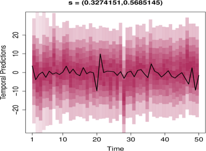
(a) Spatial index $1$.

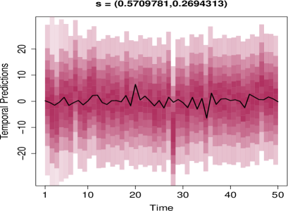
(b) Spatial index $5$.

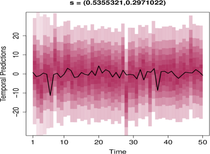
(c) Spatial index $10$.

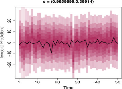
(d) Spatial index $15$.

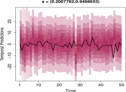
(e) Spatial index $19$.

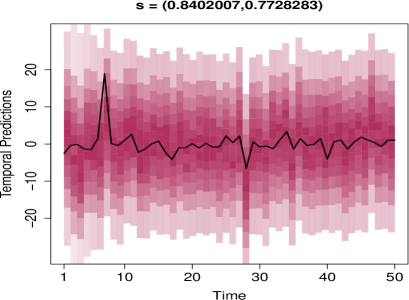
(f) Spatial index $20$.

Figure 3: Simulation study: posterior temporal predictions at various spatial locations $\boldsymbol{s}$ are shown as colour plots with progressively higher densities depicted by progressively intense colours.

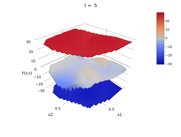
(a) Temporal index $5$.

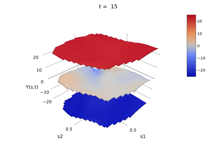
(b) Temporal index $10$.

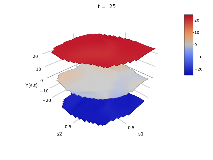
(c) Temporal index $20$.

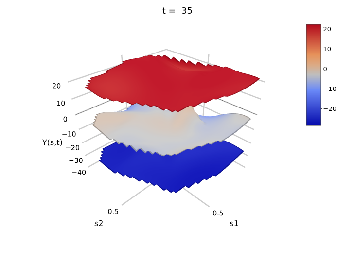
(d) Temporal index $30$.

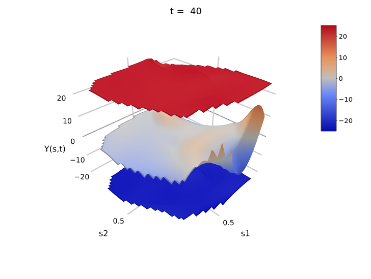
(e) Temporal index $40$.

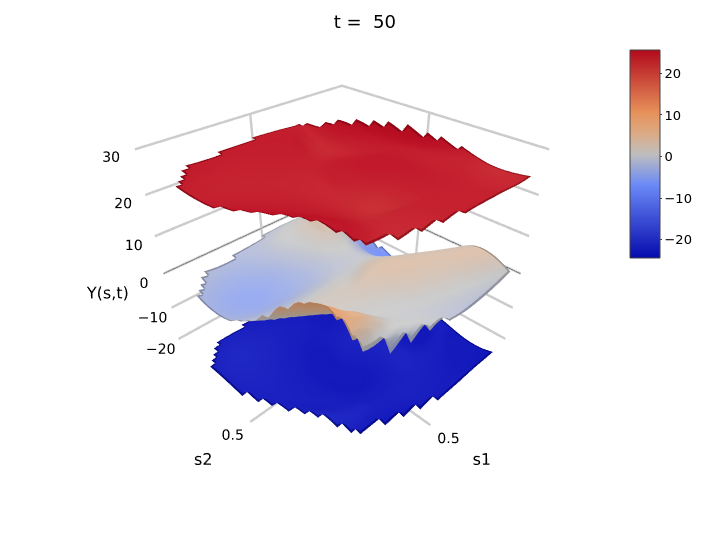
(f) Temporal index $50$.

Figure 4: Simulation study: posterior spatial predictions at various time points $t$. The middle surface is the actual spatial data, while the lower and upper surfaces are the lower and upper bounds of the $0.875$ credible region.

Figure 4 shows the spatial surface plots at various time points. The middle surface is the actual spatial surface (supplemented by spline-based interpolations), while the lower and upper surfaces (again, supplemented by spline-based interpolations) are the lower and upper bounds, respectively, of the $0.875$ credible region. In other words, the lower and upper surfaces correspond to $1/16$-th and $15/16$-th quantiles of the respective posterior predictive distributions. The detailed spatial posterior predictive densities are shown in Figure 5, as color plots akin to the temporal color plots of Figure 3, with spatial indices replacing the time indices. Unlike the time points, no ordering is intended with respect to the spatial indices. That is, we simply refer to $i=1,\ldots,20$, as the spatial indices associated with $\boldsymbol{s}_{i}$. Thus, it is evident from the figures that almost all the actual spatial data fall within the high-density regions of the corresponding posterior predictive distributions. However, again for some time points, there are a few spatial data points that are highly positive or negative, and our predictions failed in such cases (not shown).

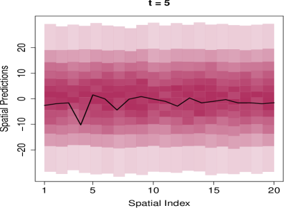
(a) Temporal index $5$.

(b) Temporal index $15$.

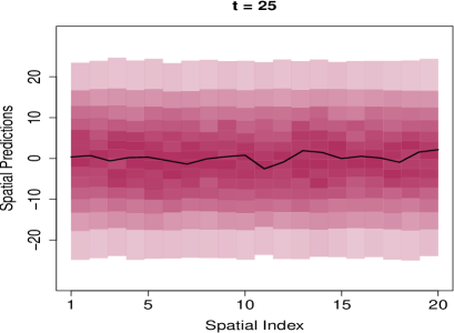
(c) Temporal index $25$.

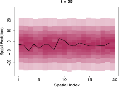
(d) Temporal index $35$.

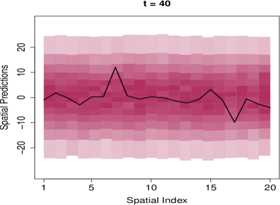
(e) Temporal index $40$.

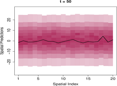
(f) Temporal index $50$.

Figure 5: Simulation study: posterior spatial predictions with respect to spatial indices at the time points $t$ as in Figure 4 are shown as colour plots with progressively higher densities depicted by progressively intense colours.

9.4 Faster implementation after integrating out the random effects

Note that simulation of $\boldsymbol{\phi}$, although parallelised, requires many parallel processors for efficiency if either $n$ or $m$ is even moderately large. As already reported in Section 9.1, this constitutes significant communication overhead among the processors and slows down implementation. Redundancy of the cores is also a consequence in the case of moderately large datasets. On the other hand, for significantly large datasets with a large number of time points, a large number of parallel processors are necessary for efficiency. However, such large number of processors are usually not available.

To get around this problem, for $i=1,\ldots,n$ and $k=1,\ldots,m$, we invoke the marginalized model (17) and the discussion thereafter and set $\phi(\boldsymbol{s}_{i},t_{k})=\phi_{0}(\boldsymbol{s}_{i},t_{k})$, provided the posterior uncertainties in $\phi(\boldsymbol{s}_{i},t_{k})$ are negligible. Since the prior distributions of $\phi(\boldsymbol{s}_{i},t_{k})$ are concentrated around $\phi_{0}(\boldsymbol{s}_{i},t_{k})$ (recall that $\sigma^{2}_{\phi}$ is concentrated around zero a priori), our experiments reveal that this is indeed the case (not shown for brevity).

To justify our standpoint, we conduct a further experiment by setting $\phi(\boldsymbol{s}_{i},t_{k})=\phi_{0}(\boldsymbol{s}_{i},t_{k})$ in our model. Not only does the time taken reduce to just $24$ minutes from $1$ hour $27$ minutes with $25$ cores, but the prediction results with this setup (see Figures 6, 7 and 8 are remarkably similar to those in the previous non-marginalized implementation (Figures 3, 4 and 5).

In this case, the average TTMCMC acceptance rates of the birth, death and no-change moves over $50$ time points are approximately $0.103$, $0.673$ and $0.617$, respectively, and the average overall TTMCMC acceptance rate is $0.420$. The TMCMC step has acceptance rate $0.017$, and that of the mixing-enhancement step is $0.152$. Thus, compared to the non-marginalized model, here the acceptance rates of the TMCMC and the mixing-enhancement steps have significantly decreased, but this is not a strong enough reason for concern since both the models yield remarkably similar performances with respect to our main goal, Bayesian prediction.

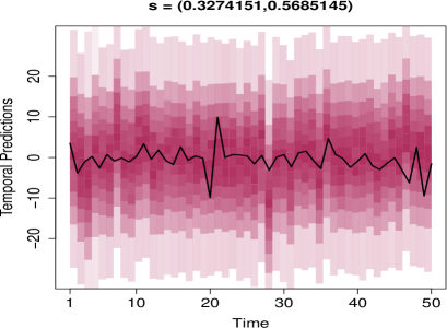
(a) Spatial index $1$.

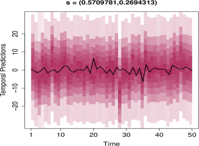
(b) Spatial index $5$.

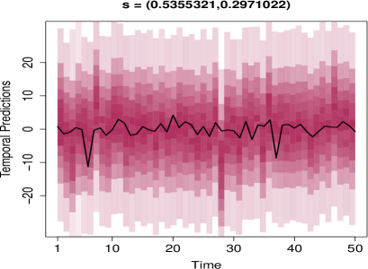
(c) Spatial index $10$.

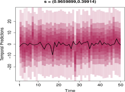
(d) Spatial index $15$.

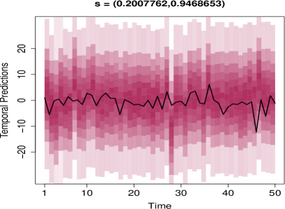
(e) Spatial index $19$.

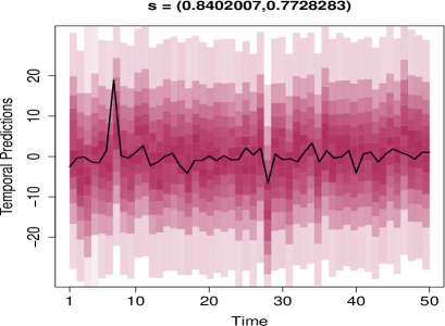
(f) Spatial index $20$.

Figure 6: Simulation study: posterior temporal predictions assuming $\phi(\boldsymbol{s}_{i},t_{k})=\phi_{0}(\boldsymbol{s}_{i},t_{k})$ for $i=1,\ldots,n$ and $k=1,\ldots,m$.

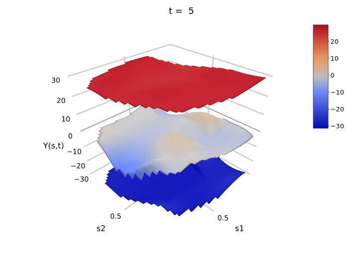
(a) Temporal index $5$.

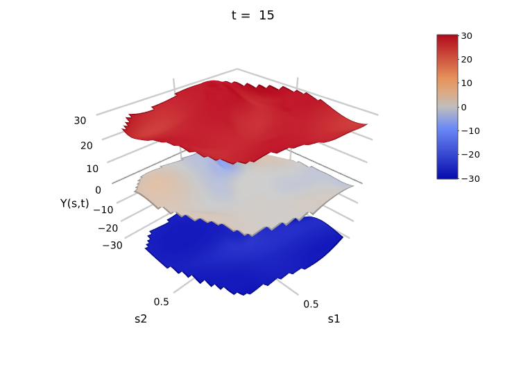
(b) Temporal index $10$.

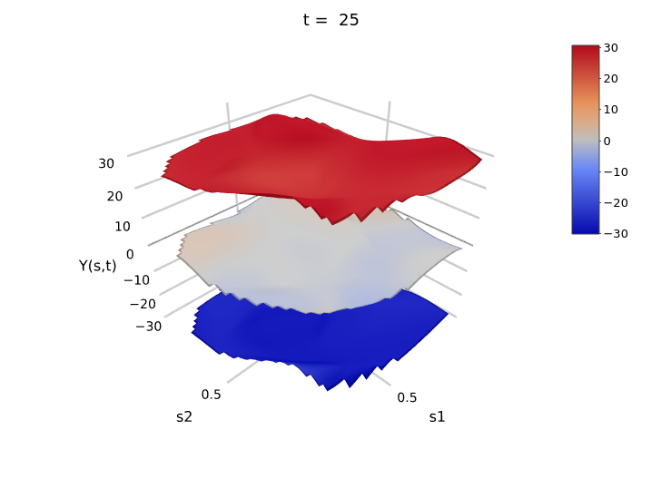
(c) Temporal index $20$.

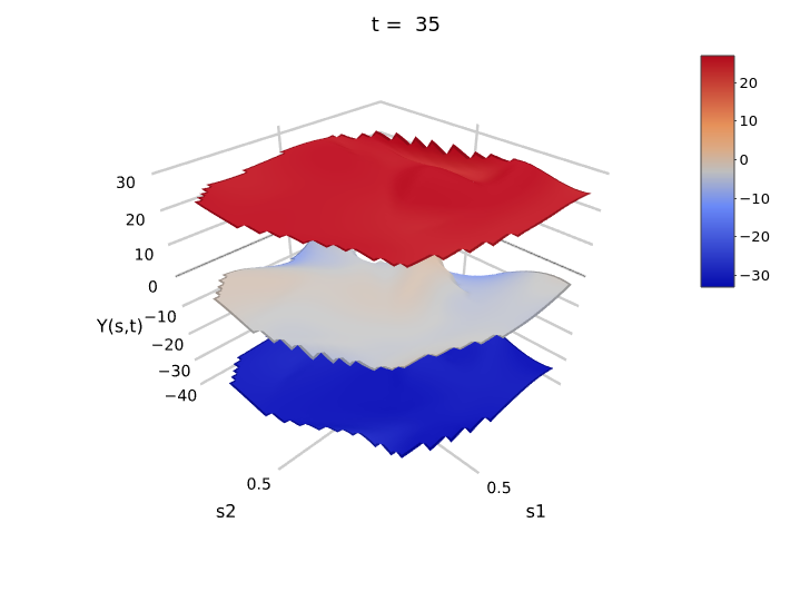
(d) Temporal index $30$.

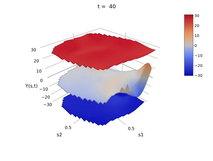
(e) Temporal index $40$.

(f) Temporal index $50$.

Figure 7: Simulation study: posterior spatial predictions at various time points $t$ assuming $\phi(\boldsymbol{s}_{i},t_{k})=\phi_{0}(\boldsymbol{s}_{i},t_{k})$ for $i=1,\ldots,n$ and $k=1,\ldots,m$.

(a) Temporal index $5$.

(b) Temporal index $15$.

(c) Temporal index $25$.

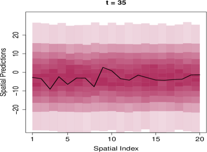
(d) Temporal index $35$.

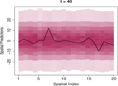
(e) Temporal index $40$.

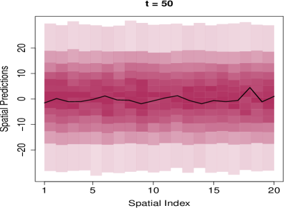
(f) Temporal index $50$.

Figure 8: Simulation study: posterior spatial predictions with respect to spatial indices at the time points $t$ as in Figure 7 assuming $\phi(\boldsymbol{s}_{i},t_{k})=\phi_{0}(\boldsymbol{s}_{i},t_{k})$ for $i=1,\ldots,n$ and $k=1,\ldots,m$.

10 Analysis of sea surface temperature data

We now consider analysis of a real, sea surface temperature dataset available at http://iridl.ldeo.columbia.edu/SOURCES/.CAC/ in the netCDF file format. The data pertains to monthly sea surface temperatures during January $1970$ – December $2003$ at the tropical Pacific Ocean region covering $124\degree E-70\degree W$ and $30\degree S-30\degree N$, gridded at a $2\degree$ by $2\degree$ resolution. Analysis of a somewhat similar (and much smaller) dataset has been reported in Cressie and Wikle (2011), on the basis of some simple linear and non-linear dynamic state-space models, but that data represented monthly temperature anomalies from the normal, rather than the actual temperatures. The models of Cressie and Wikle (2011) are not intended to cover enough grounds like ours, namely, weak and strong nonstationarity, non-separability, nonparametric non-Gaussianity and convergence of the lagged correlations to zero. Nevertheless, the simplicity of their models enabled them to perform simple Gibbs sampling based Bayesian analysis, for both of their linear and nonlinear dynamic models. However, the samplers are run for only $6000$ MCMC iterations (the first $1000$ discarded as burn-in). Wikle et al. (2019) also consider the anomalies dataset for some simplistic spatio-temporal analyses.

Our dataset consists of space-time data at $n=2520$ spatial locations, for each of $m=398$ time points. That is, the size of our dataset is $nm=10,02,960$. Figure 9 displays the sea surface temperature plots during January $1989$, $1993$ and $1998$ to exhibit the effects of La Niña (colder than normal temperatures), normal temperatures and El Niño (warmer than normal temperatures), respectively. Wikle et al. (2019) provide similar plots in essence with their anomalies data using different colouring schemes in the R package, as opposed to ours in Python, in the context of the actual temperatures.

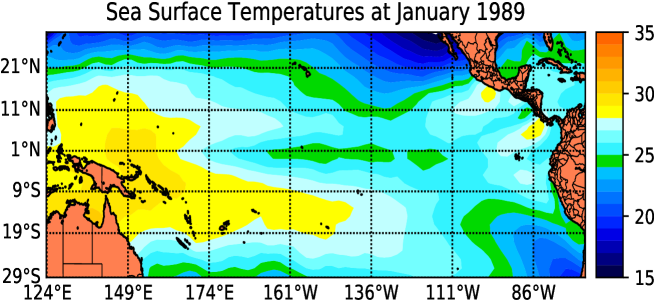
(a) La Niña (colder than normal temperatures).

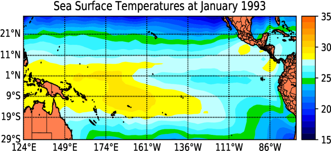
(b) Normal temperatures.

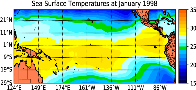
(c) El Niño (warmer than normal temperatures).

Figure 9: Sea surface temperature plots in January 1898, 1993 and 1998.

10.1 Spatio-temporal nonstationarity of the sea surface temperature data

In real life situations, the assumption of stationarity, or even covariance stationarity of the underlying spatio-temporal process, are usually too naive to be realistic. In our case, Figure 9 alone vindicates that for different time points, the spatial distributions of temperature are different, thus empirically ruling out stationarity. Moreover, for different spatial locations, the distributions of the time series are also different, as can be observed from the thick black lines in Figure 13.

For more formal conclusion regarding nonstationarity of the sea surface temperature data, we adopt the recursive Bayesian theory and methods developed by Roy and Bhattacharya (2020) in this regard. In a nutshell, their key idea is to consider the Kolmogorov-Smirnov distance between distributions of data associated with local and global space-times. Associated with the $j$-th local space-time region is an unknown probability $p_{j}$ of the event that the underlying process is stationarity when the observed data corresponds to the $j$-th local region and the Kolmogorov-Smirnov distance falls below $c_{j}$, where $c_{j}$ is any non-negative sequence tending to zero as $j$ tends to infinity. With suitable priors for $p_{j}$, Roy and Bhattacharya (2020) constructed recursive posterior distributions for $p_{j}$ and proved that the underlying process is stationary if and only if for sufficiently large number of observations in the $j$-th region, the posterior of $p_{j}$ converges to one as $j\rightarrow\infty$. Nonstationarity is the case if and only if the posterior of $p_{j}$ converges to zero as $j\rightarrow\infty$.

Covariance stationarity has been treated by Roy and Bhattacharya (2020) using similar principles, replacing the local and global distributions by local and global covariances of spatio-temporal lag $\|\boldsymbol{h}\|$, where $\boldsymbol{h}$ is the difference between the spatial-temporal co-ordinates, and $\|\cdot\|$ is the Euclidean distance. The process is covariance stationarity if and only if for sufficiently large number of observations in the $j$-th region, the posterior of $p_{j}$ converges to one as $j\rightarrow\infty$, for all $\|\boldsymbol{h}\|>0$. On the other hand, the process is covariance nonstationary if and only if there exists $\|\boldsymbol{h}\|>0$ such that the posterior of $p_{j}$ converges to zero as $j\rightarrow\infty$.

In our implementation of the ideas of Roy and Bhattacharya (2020), we set the $j$-th local region to be the entire time series for the spatial location $\boldsymbol{s}_{j}$, for $j=1,\ldots,2520$. Thus, the size of each local region is $398$, which is sufficiently large for our purpose. The number of regions, $2520$, is also large enough for the Bayesian recursive theories to be applicable. To check stationarity, we choose $c_{j}$ to be of the same nonparametric, dynamic and adaptive form as detailed in Roy and Bhattacharya (2020). The dynamic form requires an initial value for the sequence. It is important to remark here that in practice, the choice of the initial value has significant effect on the convergence of the posteriors of $p_{j}$, and hence such a choice must be carefully made. However, in our case, for such a large dataset we expect initial values even close enough to zero to suffice for inferring stationarity if the underlying phenomenon is indeed stationary. As it turned out, for all initial values less than or equal to $0.26$, the recursive Bayesian procedure led to the conclusion of nonstationarity of the underlying spatio-temporal process.

We implemented the idea with our parallelised C code on $2$ parallel processors of our ordinary laptop; the time taken is just $2$ seconds. For the initial value $0.26$, Figure 10 displays the means of the posteriors of $p_{j}$; $j=1,\ldots,2520$, showing clear convergence to zero. The respective posterior variances are negligibly small and hence not shown. Thus, as already anticipated, the spatio-temporal process that generated the sea surface temperature data, can be safely regarded as nonstationary.

Figure 11 shows the results of our investigation of covariance stationarity. Panels (b), (c), (e) and (f) show convergence of the posterior means of $p_{j}$ in this context to zero for different partitioned intervals of $\|\boldsymbol{h}\|$ associated with sufficient data such that the covariances are well-defined. The posterior variances are again negligibly small as before. Thus, covariance nonstationarity of the underlying spatio-temporal process is also clearly indicated. In these cases, we chose the initial values of $c_{j}$ to be $0.05$. The time taken for our parallelised C code implementation on our dual-core laptop is only $5$ seconds for each $\|\boldsymbol{h}\|$. Hence, the sea surface temperature phenomenon is not even weakly stationary.

Figure 10: Real data analysis: detection of strict nonstationarity.

(a) $0\leq\|\boldsymbol{h}\|<1.5$.

(b) $1.5\leq\|\boldsymbol{h}\|<2.5$.

(c) $2.5\leq\|\boldsymbol{h}\|<3.5$.

(d) $3.5\leq\|\boldsymbol{h}\|<4.5$.

(e) $4.5\leq\|\boldsymbol{h}\|<5.5$

(f) $5.5\leq\|\boldsymbol{h}\|<6.5$.

Figure 11: Real data analysis: detection of covariance nonstationarity.

10.2 Convergence of lagged spatio-temporal correlations to zero

Recall that two major purposes of our Lévy-dynamic spatio-temporal model is to account for nonstationarity of most real-life data and to emulate the property of most real datasets that the lagged spatio-temporal correlations tend to zero as the spatio-temporal lag $\|\boldsymbol{h}\|$ tends to infinity, in spite of nonstationarity. For the sea surface temperature dataset, we have already confirmed strict nonstationarity as well as covariance nonstationarity. It now remains to address the issue of the lagged correlations.

For our purpose, we randomly select $25$ spatial locations and consider the entire time series associated with each of them. We further augment the data with the first $50$ time points of another random location, thus yielding a dataset of size $10,000$. We compute the lagged correlations on $80$ parallel processors on our VMWare, each processor computing the correlation for a partitioned interval of lag $\|\boldsymbol{h}\|$ such that the interval is associated with sufficient data making the correlation well-defined. The time taken for this exercise is about $3$ minutes.

Figure 12 shows that with respect to this real dataset, our expectation that the lagged spatio-temporal correlations converge to zero in spite of nonstationarity, is not unfounded. Further experiments with larger data sizes, but with much longer implementation times, corroborated this result.

Figure 12: Real data analysis: lagged spatio-temporal correlations converging to zero.

10.3 Non-Gaussianity of the sea surface temperature data

Simple quantile-quantile plots (not shown for brevity) revealed that the distributions of the time series data at the spatial locations, distributions of the spatial data at the time points, and the overall distribution of the entire dataset, are far from normal. Thus, traditional Gaussian process based models of the underlying spatio-temporal process are ruled out. Since the temporal distributions at the spatial locations and the spatial distributions at different time points are also much different, it does not appear feasible to consider parametric stochastic process models for the data. In this regard as well, relevance of our nonparametric Lévy-dynamic process is quite pronounced.

In other words, we have validated that the underlying spatio-temporal process that generated the sea surface temperature data is non-Gaussian, strictly and weakly nonstationary, and the lagged correlations converge to zero as the lags tend to infinity. Moreover, there is no reason to traditionally assume separability of the spatio-temporal covariance structure. Since our nonparametric Lévy-dynamic process is endowed with all the aforementioned characteristics, it seems to be a very appropriate candidate for analysing the data.

10.4 Bayesian Lévy-dynamic model implementation and results

The current computational resources at Indian Statistical Institute are certainly not adequate for analysing the entire sea surface temperature dataset within a reasonable time frame. Hence, we randomly chose $300$ spatial locations and the entire time series associated with each of them. Thus, our selected subsample consists of $119,400$ spatio-temporal observations, which is not a small dataset with respect to our sophisticated Bayesian hierarchical modeling framework with complex dependence structures. Indeed, we are not aware of application of realistically sophisticated Bayesian hierarchical models to spatio-temporal datasets as large. We further randomly choose another set of $50$ locations from the remaining set of locations and the corresponding time series data of size $398$ for each location for evaluation of the predictive performance of our model. As before, we standardize the dataset and report the prediction results after transforming them back to the original location and scale.

Simplification of the structure induced by the spatio-temporal random effects by setting $\phi(\boldsymbol{s}_{i},t_{k})=\phi_{0}(\boldsymbol{s}_{i},t_{k})$ for $i=1,\ldots,n=300$ and $k=1,\ldots,m=398$ (for training) and $\phi(\tilde{\boldsymbol{s}}_{i},t_{k})=\phi_{0}(\tilde{\boldsymbol{s}}_{i},t_{k})$ for $i=1,\ldots,n=50$ and $k=1,\ldots,m=398$ (for prediction) in our marginalized Lévy-dyanmic model (17) and the following discussion brought down the implementation time (on $80$ parallel processors) from more than $3$ days (estimated) to less than a single day. Here the average TTMCMC acceptance rates of the birth, death and no-change moves over $398$ time points are approximately $0.095$, $0.709$ and $0.661$, respectively, and the average overall TTMCMC acceptance rate is $0.439$. The acceptance rates for TMCMC and the mixing enhancement steps are $0.033$ and $0.03$, respectively. Note that these acceptance rates are broadly similar to those reported in the context of the simulation experiment with the marginalized random effects model (Section 9.4). Thus, the acceptance rates seem to exhibit a tendency of robustness with respect to different datasets of varying sizes.

Figure 13 shows the time series predictions at a few of the $50$ spatial locations set aside for prediction. Observe that for each spatial location, the entire true time series falls well within the associated $0.875$ posterior predictive density region. Although in panels (c) and in particularly panel (f), the time series do not pass through the highest posterior predictive density regions depicted by the most intense colours, the trends in these cases seem to be still well-captured by our Bayesian model and methods.

Figure 14 displays the spatial predictions at a few time points, in the forms of $95\%$ lower and upper Bayesian spatial prediction surfaces, while the middle, true spatial surface corresponds to the $50$ spatial locations meant for prediction. The reason for choosing $95\%$ surfaces, rather than $0.875$, as in the simulation experiments is that for many time points, the $0.875\%$ surfaces failed to capture several true spatial data points. Even the $95\%$ surfaces failed to satisfactorily contain either one or two spatial data points, for several time points (not shown for brevity). Setting $\sigma^{2}_{\phi}$ to some non-negligible positive value might have solved the issue, but would have increased the Bayesian prediction intervals for most of the other data points which are already well-captured.

Figure 15 exhibits the density based colour plots of the spatial predictions corresponding to Figure 14. In this case we use $40$ percentiles to make the figures correspond to $95\%$ credible regions, for comparability with Figure 14.

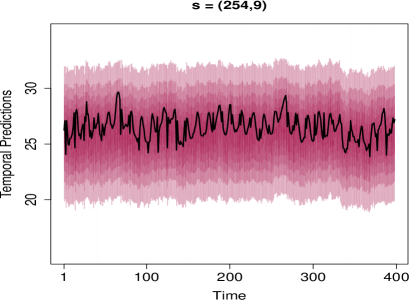
(a) Spatial index $1$.

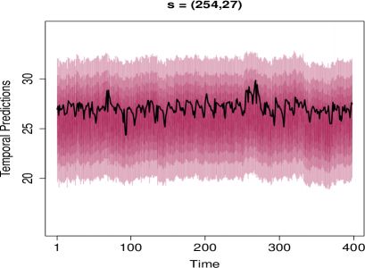
(b) Spatial index $15$.

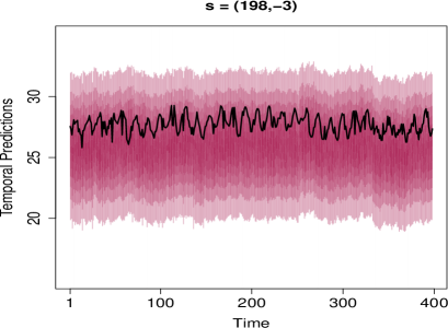
(c) Spatial index $20$.

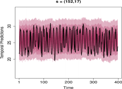
(d) Spatial index $30$.

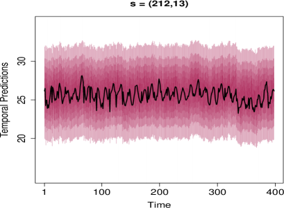
(e) Spatial index $40$.

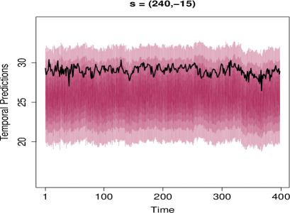
(f) Spatial index $50$.

Figure 13: Real data analysis: posterior temporal predictions.

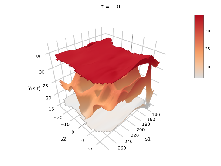
(a) Temporal index $10$.

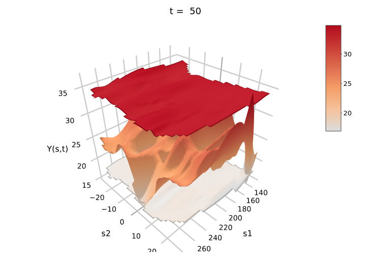
(b) Temporal index $50$.

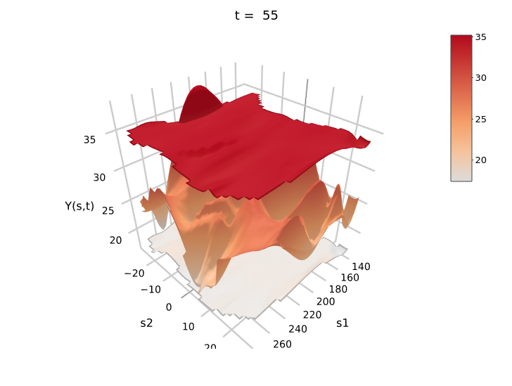
(c) Temporal index $55$.

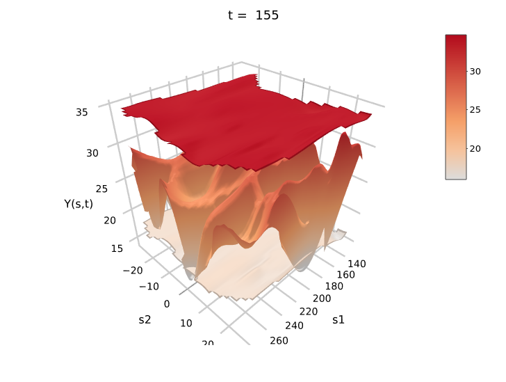
(d) Temporal index $155$.

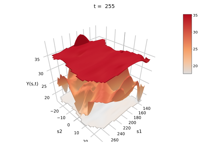
(e) Temporal index $255$.

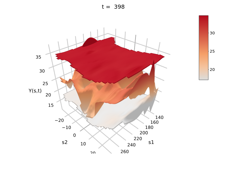
(f) Temporal index $398$.

Figure 14: Real data analysis: posterior spatial predictions at various time points $t$.

(a) Temporal index $10$.

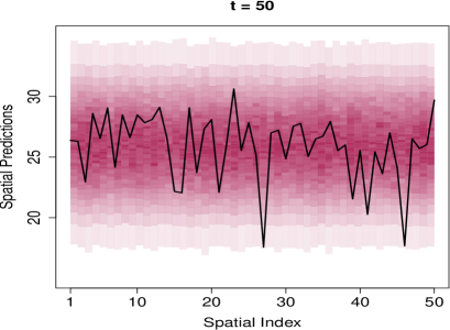
(b) Temporal index $50$.

(c) Temporal index $55$.

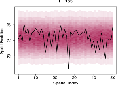
(d) Temporal index $155$.

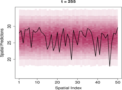
(e) Temporal index $255$.

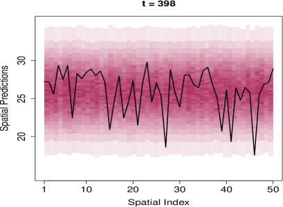
(f) Temporal index $398$.

Figure 15: Real data analysis: posterior spatial predictions with respect to spatial indices at the time points $t$ as in Figure 14.

11 Summary and conclusion

The Gaussian process is overused in the spatial/spatio-temporal literature, particularly in large data scenarios. The reality issues such as non-Gaussianity, nonstationarity, nonseparability and properties of the lagged correlations are often relegated to the background in favour of convenience, even in general data-fitting scenarios. These seem to induce some inflexibility in the current state-of-the-art spatial/spatio-temporal statistics, as even a plethora of existing Gaussian process based methods and a competition among them failed to yield analysis of any big data in the order of terabytes. The key impediment in the implementation of all such methods is matrix-based computation, which may be ameliorated, but can not be avoided. In the zest for simplifying computations in Gaussian processes, the realistic issues are often forgotten, as mentioned above.

Thus, there is a need to develop realistic spatial and spatio-temporal models and methods that satisfy the realistic properties, and are also amenable to fast and efficient matrix-free computation to meet the challenges of large data. In this regard, we introduce our Bayesian Lévy-dynamic spatio-temporal model based upon Lévy random fields, and show that it satisfies the desirable realistic properties. As we have shown, the approach is flexible enough for modeling space-time data with weak temporal dynamics or even purely spatial data.

For capturing micro-scale spatio-temporal variations, we introduce spatio-temporal random effects, which are amenable to marginalization that enormously simplify computations. The model is completely matrix-free, but is variable-dimensional with respect to each of the time indices. We handle the variable-dimensional parameters using TTMCMC and the fixed-dimensional parameters using TMCMC, all embedded in a novel parallel MCMC algorithm, which we code in C in the MPI paradigm for parallelism. The model structure allows us to update the variable-dimensional parameters for all the even (odd) time indices in parallel, followed by updating those for all odd (even) time indices. Even for fixed-dimensional updates, we compute the acceptance ratios and several other quantities in parallel. Thus, in conjunction with integrating out the random effects, our parallel MCMC algorithm leads to huge computational savings. However, the mixing properties are enhanced when the random effects are not integrated out. Despite this, the Bayesian predictions are almost unaffected by the issue of marginalization of the random effects as borne out by our simulation experiment, providing the green signal to consider the marginalized model for analysis of large datasets.

We indeed analyse a relatively large sea surface temperature dataset consisting of $139,300$ space-time observations using our marginalized Bayesian Lévy-dynamic model; the time taken being less than $24$ hours on our VMWare with $80$ cores. The encouraging results suggest that with more powerful and well-maintained computing facilities, we may ambitiously begin analyzing “big data” in the order of terabytes, without any compromise whatsoever on the theoretical properties with respect to data realism.

Supplementary Material

S-12 Proof of Theorem 1

Proof.

Let us first prove (i). Note that given $\mathbf{M}(\boldsymbol{s}_{1})$ and $\mathbf{M}(\boldsymbol{s}_{2})$, the covariance between $f(\boldsymbol{s}_{1},t)$ and $f(\boldsymbol{s}_{2},t)$ is given by

$$Cov\left(f(\boldsymbol{s}_{1},t),f(\boldsymbol{s}_{2},t)\bigg{|}\mathbf{M}(\boldsymbol{s}_{1}),\mathbf{M}(\boldsymbol{s}_{2})\right)$$

$$=Cov\left(\sum_{0\leq j<J_{t}}K(\mathbf{M}(\boldsymbol{s}_{1})-\boldsymbol{\mu}_{jt},t-\tau|\boldsymbol{\Sigma},\xi)\beta_{jt},\right.$$

$$\qquad\qquad\left.\sum_{0\leq j<J_{t}}K(\mathbf{M}(\boldsymbol{s}_{2})-\boldsymbol{\mu}_{jt_{2}},t-\tau|\boldsymbol{\Sigma},\xi)\beta_{jt}\bigg{|}\mathbf{M}(\boldsymbol{s}_{1}),\mathbf{M}(\boldsymbol{s}_{2})\right)$$

$$=E\left[Cov\left(\sum_{0\leq j<J_{t}}K(\mathbf{M}(\boldsymbol{s}_{1})-\boldsymbol{\mu}_{jt},t-\tau|\boldsymbol{\Sigma},\xi)\beta_{jt},\right.\right.$$

$$\qquad\qquad\left.\left.\sum_{0\leq j<J_{t}}K(\mathbf{M}(\boldsymbol{s}_{2})-\boldsymbol{\mu}_{jt},t-\tau|\boldsymbol{\Sigma},\xi)\beta_{jt}\bigg{|}\mathbf{M}(\boldsymbol{s}_{1}),\mathbf{M}(\boldsymbol{s}_{2}),J_{t}\right)\right]$$ (S-48)

$$\qquad+Cov\left(E\left[\sum_{0\leq j<J_{t}}K(\mathbf{M}(\boldsymbol{s}_{1})-\boldsymbol{\mu}_{jt},t-\tau|\boldsymbol{\Sigma},\xi)\beta_{jt}\bigg{|}J_{t}\right],\right.$$

$$\qquad\qquad\qquad\qquad\qquad\left.E\left[\sum_{0\leq j<J_{t}}K(\mathbf{M}(\boldsymbol{s}_{2})-\boldsymbol{\mu}_{jt},t-\tau|\boldsymbol{\Sigma},\xi)\beta_{jt}\bigg{|}J_{t}\right]\Bigg{|}\mathbf{M}(\boldsymbol{s}_{1}),\mathbf{M}(\boldsymbol{s}_{2})\right).$$ (S-49)

Now the inner covariance structure in (S-48) has the following form:

$$Cov\left(\sum_{0\leq j<J_{t}}K(\mathbf{M}(\boldsymbol{s}_{1})-\boldsymbol{\mu}_{jt},t-\tau|\boldsymbol{\Sigma},\xi)\beta_{jt},\right.$$

$$\qquad\qquad\left.\sum_{0\leq j<J_{t}}K(\mathbf{M}(\boldsymbol{s}_{2})-\boldsymbol{\mu}_{jt},t-\tau|\boldsymbol{\Sigma},\xi)\beta_{jt}\bigg{|}\mathbf{M}(\boldsymbol{s}_{1}),\mathbf{M}(\boldsymbol{s}_{2}),J_{t}\right)$$

$$=Cov\left(\boldsymbol{1}^{T}_{J_{t}}\boldsymbol{X},\boldsymbol{1}^{T}_{J_{t}}\boldsymbol{Y}\bigg{|}\mathbf{M}(\boldsymbol{s}_{1}),\mathbf{M}(\boldsymbol{s}_{2}),J_{t}\right)$$

$$=\boldsymbol{1}^{T}_{J_{t}}Cov\left(\boldsymbol{X},\boldsymbol{Y}\bigg{|}\mathbf{M}(\boldsymbol{s}_{1}),\mathbf{M}(\boldsymbol{s}_{2}),J_{t}\right)\boldsymbol{1}_{J_{t}},$$

where $\boldsymbol{1}_{J_{t}}$ is the vector consisting of $J_{t}$ elements, each element being $1$, $\boldsymbol{X}=(K(\mathbf{M}(\boldsymbol{s}_{1})-\boldsymbol{\mu}_{jt},t-\tau|\boldsymbol{\Sigma},\xi)\beta_{jt},j=0,1,\ldots,J_{t}-1)^{T}$ and $\boldsymbol{Y}=(K(\mathbf{M}(\boldsymbol{s}_{2})-\boldsymbol{\mu}_{jt},t-\tau|\boldsymbol{\Sigma},\xi)\beta_{jt},j=0,1,\ldots,J_{t}-1)^{T}$. Since

$$Cov(\boldsymbol{X},\boldsymbol{Y}\bigg{|}\mathbf{M}(\boldsymbol{s}_{1}),\mathbf{M}(\boldsymbol{s}_{2}),J_{t})$$

$$=Cov\left(K(\mathbf{M}(\boldsymbol{s}_{1})-\boldsymbol{\mu}_{t},t-\tau|\boldsymbol{\Sigma},\xi)\beta_{t},K(\mathbf{M}(\boldsymbol{s}_{2})-\boldsymbol{\mu}_{t},t-\tau|\boldsymbol{\Sigma},\xi)\beta_{t}\bigg{|}\mathbf{M}(\boldsymbol{s}_{1}),\mathbf{M}(\boldsymbol{s}_{2})\right)\boldsymbol{I}_{J_{t}},$$

where $\boldsymbol{I}_{J_{t}}$ is the $J_{t}\times J_{t}$ identity matrix,

$$\boldsymbol{1}^{T}_{J_{t}}Cov\left(\boldsymbol{X},\boldsymbol{Y}\bigg{|}\mathbf{M}(\boldsymbol{s}_{1}),\mathbf{M}(\boldsymbol{s}_{2}),J_{t}\right)\boldsymbol{1}_{J_{t}}$$

$$=J_{t}Cov\left(K(\mathbf{M}(\boldsymbol{s}_{1})-\boldsymbol{\mu}_{t},t-\tau|\boldsymbol{\Sigma},\xi)\beta_{t},K(\mathbf{M}(\boldsymbol{s}_{2})-\boldsymbol{\mu}_{t},t-\tau|\boldsymbol{\Sigma},\xi)\beta_{t}\bigg{|}\mathbf{M}(\boldsymbol{s}_{1}),\mathbf{M}(\boldsymbol{s}_{2}),J_{t}\right).$$

Hence, (S-48) is equal to

$$E\left[\boldsymbol{1}^{T}_{J_{t}}Cov\left(\boldsymbol{X},\boldsymbol{Y}\bigg{|}\mathbf{M}(\boldsymbol{s}_{1}),\mathbf{M}(\boldsymbol{s}_{2}),J_{t}\right)\boldsymbol{1}_{J_{t}}\right]$$

$$=\lambda Cov\left(K(\mathbf{M}(\boldsymbol{s}_{1})-\boldsymbol{\mu}_{t},t-\tau|\boldsymbol{\Sigma},\xi)\beta_{t},K(\mathbf{M}(\boldsymbol{s}_{2})-\boldsymbol{\mu}_{t},t-\tau|\boldsymbol{\Sigma},\xi)\beta_{t}\bigg{|}\mathbf{M}(\boldsymbol{s}_{1}),\mathbf{M}(\boldsymbol{s}_{2})\right)$$

$$=\lambda E\left[K(\mathbf{M}(\boldsymbol{s}_{1})-\boldsymbol{\mu}_{t},t)K(\mathbf{M}(\boldsymbol{s}_{2})-\boldsymbol{\mu}_{t},t-\tau|\boldsymbol{\Sigma},\xi)\beta^{2}_{t}\bigg{|}\mathbf{M}(\boldsymbol{s}_{1}),\mathbf{M}(\boldsymbol{s}_{2})\right]$$

$$\qquad-\lambda E\left[K(\mathbf{M}(\boldsymbol{s}_{1})-\boldsymbol{\mu}_{t},t-\tau|\boldsymbol{\Sigma},\xi)\beta_{t}\bigg{|}\mathbf{M}(\boldsymbol{s}_{1})\right]E\left[K(\mathbf{M}(\boldsymbol{s}_{2})-\boldsymbol{\mu}_{t},t-\tau|\boldsymbol{\Sigma},\xi)\beta_{t}\bigg{|}\mathbf{M}(\boldsymbol{s}_{2})\right].$$ (S-50)

Let us now consider the term (S-49). Note that for any $\boldsymbol{s}\in\mathbb{R}^{p}$,

$$E\left[\sum_{0\leq j<J_{t}}K(\mathbf{M}(\boldsymbol{s})-\boldsymbol{\mu}_{jt},t-\tau|\boldsymbol{\Sigma},\xi)\beta_{jt}\bigg{|}\mathbf{M}(\boldsymbol{s}),J_{t}\right]=J_{t}E\left[K(\mathbf{M}(\boldsymbol{s})-\boldsymbol{\mu}_{t},t-\tau|\boldsymbol{\Sigma},\xi)\beta_{t}\bigg{|}\mathbf{M}(\boldsymbol{s})\right].$$ (S-51)

Hence, (S-49) is given by

$$Cov\left(J_{t}E\left[K(\mathbf{M}(\boldsymbol{s}_{1})-\boldsymbol{\mu}_{t},t-\tau|\boldsymbol{\Sigma},\xi)\beta_{t}\right],J_{t}E\left[K(\mathbf{M}(\boldsymbol{s}_{2})-\boldsymbol{\mu}_{t},t-\tau|\boldsymbol{\Sigma},\xi)\beta_{t}\right]\bigg{|}\mathbf{M}(\boldsymbol{s}_{1}),\mathbf{M}(\boldsymbol{s}_{2})\right)$$

$$=\lambda E\left[K(\mathbf{M}(\boldsymbol{s}_{1})-\boldsymbol{\mu}_{t},t-\tau|\boldsymbol{\Sigma},\xi)\beta_{t}\bigg{|}\mathbf{M}(\boldsymbol{s}_{1})\right]E\left[K(\mathbf{M}(\boldsymbol{s}_{2})-\boldsymbol{\mu}_{t},t-\tau|\boldsymbol{\Sigma},\xi)\beta_{t}\bigg{|}\mathbf{M}(\boldsymbol{s}_{2})\right].$$ (S-52)

From (S-50) and (S-52) we obtain

$$Cov\left(f(\boldsymbol{s}_{1},t),f(\boldsymbol{s}_{2},t)\bigg{|}\mathbf{M}(\boldsymbol{s}_{1}),\mathbf{M}(\boldsymbol{s}_{2})\right)$$

$$=\lambda E\left[K(\mathbf{M}(\boldsymbol{s}_{1})-\boldsymbol{\mu}_{t},t-\tau|\boldsymbol{\Sigma},\xi)K(\mathbf{M}(\boldsymbol{s}_{2})-\boldsymbol{\mu}_{t},t-\tau|\boldsymbol{\Sigma},\xi)\beta^{2}_{t}\bigg{|}\mathbf{M}(\boldsymbol{s}_{1}),\mathbf{M}(\boldsymbol{s}_{2})\right].$$ (S-53)

Applying change-of-variable $\boldsymbol{\mu}_{t}\mapsto\mathbf{M}(\boldsymbol{s}_{2})-\boldsymbol{\mu}_{t}$ to the expectation (S-53) shows that the expectation is a function of $\mathbf{M}(\boldsymbol{s}_{1})-\mathbf{M}(\boldsymbol{s}_{2})$. If the elements of $\mathbf{M}(\cdot)$ are Lévy subordinators, the distribution of $\mathbf{M}(\boldsymbol{s}_{1})-\mathbf{M}(\boldsymbol{s}_{2})$ is the same as that of $\mathbf{M}(\boldsymbol{s}_{1}-\boldsymbol{s}_{2})$. In general, we allow the distribution of $\mathbf{M}(\boldsymbol{s}_{1})-\mathbf{M}(\boldsymbol{s}_{2})$ to depend upon $\boldsymbol{s}_{1}-\boldsymbol{s}_{2}$, so that

$$E\left[Cov\left(f(\boldsymbol{s}_{1},t),f(\boldsymbol{s}_{2},t)\bigg{|}\mathbf{M}(\boldsymbol{s}_{1}),\mathbf{M}(\boldsymbol{s}_{2})\right)\right]=g(\boldsymbol{s}_{1}-\boldsymbol{s}_{2}),$$ (S-54)

for some function $g(\cdot)$.

Now, taking expectation of both sides of (S-51) yields

$$E\left[f(\boldsymbol{s},t)\bigg{|}\mathbf{M}(\boldsymbol{s})\right]=\lambda E\left[K(\mathbf{M}(\boldsymbol{s})-\boldsymbol{\mu}_{t},t-\tau|\boldsymbol{\Sigma},\xi)\beta_{t}\bigg{|}\mathbf{M}(\boldsymbol{s})\right],$$

for any $\boldsymbol{s}\in\mathbb{R}^{p}$. Hence,

$$Cov\left(E\left[f(\boldsymbol{s}_{1},t)\bigg{|}\mathbf{M}(\boldsymbol{s}_{1})\right],E\left[f(\boldsymbol{s}_{2},t)\bigg{|}\mathbf{M}(\boldsymbol{s}_{2})\right]\right)$$

$$=\lambda^{2}E\left[E\left(K(\mathbf{M}(\boldsymbol{s}_{1})-\boldsymbol{\mu}_{t},t-\tau|\boldsymbol{\Sigma},\xi)\beta_{t}\bigg{|}\mathbf{M}(\boldsymbol{s}_{1})\right)\right.$$

$$\qquad\qquad\left.\times E\left(K(\mathbf{M}(\boldsymbol{s}_{2})-\boldsymbol{\mu}_{t},t-\tau|\boldsymbol{\Sigma},\xi)\beta_{t}\bigg{|}\mathbf{M}(\boldsymbol{s}_{2})\right)\right]$$

$$\qquad\qquad-\lambda^{2}E\left[K(\mathbf{M}(\boldsymbol{s}_{1})-\boldsymbol{\mu}_{t},t-\tau|\boldsymbol{\Sigma},\xi)\beta_{t}\right]E\left[K(\mathbf{M}(\boldsymbol{s}_{2})-\boldsymbol{\mu}_{t},t-\tau|\boldsymbol{\Sigma},\xi)\beta_{t}\right].$$ (S-55)

At least the second term of (S-55) is not a function of $\boldsymbol{s}_{1}-\boldsymbol{s}_{2}$. Hence, it follows from (S-53), (S-54) and (S-55) that

$$Cov\left(f(\boldsymbol{s}_{1},t),f(\boldsymbol{s}_{2},t)\right)$$

$$=E\left[Cov\left(f(\boldsymbol{s}_{1},t),f(\boldsymbol{s}_{2},t)\bigg{|}\mathbf{M}(\boldsymbol{s}_{1}),\mathbf{M}(\boldsymbol{s}_{2})\right)\right]$$

$$\qquad\qquad+Cov\left(E\left[f(\boldsymbol{s}_{1},t)\bigg{|}\mathbf{M}(\boldsymbol{s}_{1})\right],E\left[f(\boldsymbol{s}_{2},t)\bigg{|}\mathbf{M}(\boldsymbol{s}_{2})\right]\right)$$

does not depend upon $\boldsymbol{s}_{1}$ and $\boldsymbol{s}_{2}$ only through $\boldsymbol{s}_{1}-\boldsymbol{s}_{2}$. This proves (i).

To prove (ii), note that for any $\boldsymbol{s}\in\mathbb{R}^{p}$,

$$Cov\left(f(\boldsymbol{s},t_{1}),f(\boldsymbol{s},t_{2})\bigg{|}\mathbf{M}(\boldsymbol{s})\right)$$

$$=Cov\left(\sum_{0\leq j<J_{t_{1}}}K(\mathbf{M}(\boldsymbol{s})-\boldsymbol{\mu}_{jt_{1}},t_{1}-\tau|\boldsymbol{\Sigma},\xi)\beta_{jt_{1}},\right.$$

$$\qquad\qquad\left.\sum_{0\leq j<J_{t_{2}}}K(\mathbf{M}(\boldsymbol{s})-\boldsymbol{\mu}_{jt_{2}},t_{2}-\tau|\boldsymbol{\Sigma},\xi)\beta_{jt_{2}}\bigg{|}\mathbf{M}(\boldsymbol{s})\right)$$

$$=E\left[Cov\left(\sum_{0\leq j<J_{t_{1}}}K(\mathbf{M}(\boldsymbol{s})-\boldsymbol{\mu}_{jt_{1}},t_{1}-\tau|\boldsymbol{\Sigma},\xi)\beta_{jt_{1}},\right.\right.$$

$$\qquad\qquad\left.\left.\sum_{0\leq j<J_{t_{2}}}K(\mathbf{M}(\boldsymbol{s})-\boldsymbol{\mu}_{jt_{2}},t_{2}-\tau|\boldsymbol{\Sigma},\xi)\beta_{jt_{2}}\bigg{|}\mathbf{M}(\boldsymbol{s}),J_{t_{1}},J_{t_{2}}\right)\right]$$ (S-56)

$$\qquad+Cov\left(E\left[\sum_{0\leq j<J_{t_{1}}}K(\mathbf{M}(\boldsymbol{s})-\boldsymbol{\mu}_{jt_{1}},t_{1}-\tau|\boldsymbol{\Sigma},\xi)\beta_{jt_{1}}\bigg{|}\mathbf{M}(\boldsymbol{s}),J_{t_{1}}\right],\right.$$

$$\qquad\qquad\qquad\qquad\qquad\left.E\left[\sum_{0\leq j<J_{t_{2}}}K(\mathbf{M}(\boldsymbol{s})-\boldsymbol{\mu}_{jt_{2}},t_{2}-\tau|\boldsymbol{\Sigma},\xi)\beta_{jt_{2}}\bigg{|}\mathbf{M}(\boldsymbol{s}),J_{t_{2}}\right]\right).$$ (S-57)

First note that

$$E\left[\sum_{0\leq j<J_{t}}K(\mathbf{M}(\boldsymbol{s})-\boldsymbol{\mu}_{jt},t-\tau|\boldsymbol{\Sigma},\xi)\beta_{jt}\bigg{|}\mathbf{M}(\boldsymbol{s}),J_{t_{1}}\right]=J_{t}E\left[K(\mathbf{M}(\boldsymbol{s})-\boldsymbol{\mu}_{t},t-\tau|\boldsymbol{\Sigma},\xi)\beta_{t}\right],$$

for any $t$. Hence, the covariance term (S-57) is

$$Cov\left(J_{t_{1}}E\left[K(\mathbf{M}(\boldsymbol{s})-\boldsymbol{\mu}_{t_{1}},t_{1}-\tau|\boldsymbol{\Sigma},\xi)\beta_{t_{1}}\right],J_{t_{2}}E\left[K(\mathbf{M}(\boldsymbol{s})-\boldsymbol{\mu}_{t_{2}},t_{2}-\tau|\boldsymbol{\Sigma},\xi)\beta_{t_{2}}\right]\right)=0,$$ (S-58)

since $J_{t_{1}}$ and $J_{t_{2}}$ are independent.

In (S-56), the covariance is given by $\boldsymbol{1}^{T}_{J_{t_{1}}}Cov(\boldsymbol{X},\boldsymbol{Y}\big{|}\mathbf{M}(\boldsymbol{s}),J_{t_{1}},J_{t_{2}})\boldsymbol{1}_{J_{t_{2}}}$, where

$$\boldsymbol{X}=\left(K(\mathbf{M}(\boldsymbol{s})-\boldsymbol{\mu}_{jt_{1}},t_{1}-\tau|\boldsymbol{\Sigma},\xi)\beta_{jt_{1}},j=0,1,\ldots,J_{t_{1}}-1\right)$$

and

$$\boldsymbol{Y}=\left(K(\mathbf{M}(\boldsymbol{s})-\boldsymbol{\mu}_{jt_{2}},t_{2}-\tau|\boldsymbol{\Sigma},\xi)\beta_{jt_{2}},j=0,1,\ldots,J_{t_{2}}-1\right).$$

Hence, $\boldsymbol{1}^{T}_{J_{t_{1}}}Cov(\boldsymbol{X},\boldsymbol{Y}\big{|}\mathbf{M}(\boldsymbol{s}),J_{t_{1}},J_{t_{2}})\boldsymbol{1}_{J_{t_{2}}}$ simplifies to

$$Cov\left(K(\mathbf{M}(\boldsymbol{s})-\boldsymbol{\mu}_{t_{1}},t_{1}-\tau|\boldsymbol{\Sigma},\xi)\beta_{t_{1}},K(\mathbf{M}(\boldsymbol{s})-\boldsymbol{\mu}_{t_{2}},t_{2}-\tau|\boldsymbol{\Sigma},\xi)\beta_{t_{2}}\big{|}\mathbf{M}(\boldsymbol{s}),J_{t_{1}},J_{t_{2}}\right)$$

$$\qquad\qquad\times\min\{J_{t_{1}},J_{t_{2}}\}.$$

Consequently, (S-56) is given by

$$Cov\left(K(\mathbf{M}(\boldsymbol{s})-\boldsymbol{\mu}_{t_{1}},t_{1}-\tau|\boldsymbol{\Sigma},\xi)\beta_{t_{1}},K(\mathbf{M}(\boldsymbol{s})-\boldsymbol{\mu}_{t_{2}},t_{2}-\tau|\boldsymbol{\Sigma},\xi)\beta_{t_{2}}\big{|}\mathbf{M}(\boldsymbol{s})\right)$$

$$\qquad\qquad\times E\left[\min\{J_{t_{1}},J_{t_{2}}\}\right].$$

Because of (S-58), $Cov\left(f(\boldsymbol{s},t_{1}),f(\boldsymbol{s},t_{2}))\bigg{|}\mathbf{M}(\boldsymbol{s})\right)$ is also the same as the above expression for (S-56). Since at least $E\left[\min\{J_{t_{1}},J_{t_{2}}\}\right]$ does not depend upon $t_{1}$ and $t_{2}$ through $t_{1}-t_{2}$, it is clear that the unconditional covariance structure $Cov\left(f(\boldsymbol{s},t_{1}),f(\boldsymbol{s},t_{2})\right)$ does not depend upon $t_{1}$ and $t_{2}$ only through $t_{1}-t_{2}$.

The proof of (iii) is similar to that of (ii) with $\boldsymbol{s}$ corresponding to $t_{1}$ and $t_{2}$ replaced by $\boldsymbol{s}_{1}$ and $\boldsymbol{s}_{2}$, respectively.

∎

S-13 Proof of Theorem 2

Proof.

Let $\boldsymbol{\Theta}=\{\boldsymbol{\mu}_{jt_{1}}:j=0,1,\ldots,J_{t_{1}}-1\}\cup\{\boldsymbol{\mu}_{jt_{2}}:j=0,1,\ldots,J_{t_{2}}-1\}\cup\{\boldsymbol{\Sigma},\tau,\xi\}$. Then

$$Cov(f(\boldsymbol{s}_{1},t_{1}),f(\boldsymbol{s}_{2},t_{2}))$$

$$=Cov\left(\sum_{0\leq j<J_{t_{1}}}K(\mathbf{M}(\boldsymbol{s}_{1})-\boldsymbol{\mu}_{jt_{1}},t_{1}-\tau|\boldsymbol{\Sigma},\xi)\beta_{jt_{1}},\sum_{0\leq j<J_{t_{2}}}K(\mathbf{M}(\boldsymbol{s}_{2})-\boldsymbol{\mu}_{jt_{2}},t_{2}-\tau|\boldsymbol{\Sigma},\xi)\beta_{jt_{2}}\right)$$

$$=E\left[Cov\left(\sum_{0\leq j<J_{t_{1}}}K(\mathbf{M}(\boldsymbol{s}_{1})-\boldsymbol{\mu}_{jt_{1}},t_{1}-\tau|\boldsymbol{\Sigma},\xi)\beta_{jt_{1}},\right.\right.$$

$$\qquad\qquad\left.\left.\sum_{0\leq j<J_{t_{2}}}K(\mathbf{M}(\boldsymbol{s}_{2})-\boldsymbol{\mu}_{jt_{2}},t_{2}-\tau|\boldsymbol{\Sigma},\xi)\beta_{jt_{2}}\bigg{|}\mathbf{M}(\boldsymbol{s}_{1}),\mathbf{M}(\boldsymbol{s}_{2}),J_{t_{1}},J_{t_{2}},\boldsymbol{\Theta}\right)\right]$$ (S-59)

$$\qquad+Cov\left(E\left[\sum_{0\leq j<J_{t_{1}}}K(\mathbf{M}(\boldsymbol{s}_{1})-\boldsymbol{\mu}_{jt_{1}},t_{1}-\tau|\boldsymbol{\Sigma},\xi)\beta_{jt_{1}}\bigg{|}\mathbf{M}(\boldsymbol{s}_{1}),J_{t_{1}},J_{t_{2}},\boldsymbol{\Theta}\right],\right.$$

$$\qquad\qquad\qquad\qquad\qquad\left.E\left[\sum_{0\leq j<J_{t_{2}}}K(\mathbf{M}(\boldsymbol{s}_{2})-\boldsymbol{\mu}_{jt_{2}},t_{2}-\tau|\boldsymbol{\Sigma},\xi)\beta_{jt_{2}}\bigg{|}\mathbf{M}(\boldsymbol{s}_{2}),J_{t_{1}},J_{t_{2}},\boldsymbol{\Theta}\right]\right).$$ (S-60)

Now let us consider (S-59) in more details. Note that the inner covariance is given by

$$Cov\left(\boldsymbol{a}^{\prime}\boldsymbol{X},\boldsymbol{b}^{\prime}\boldsymbol{Y}\bigg{|}\mathbf{M}(\boldsymbol{s}_{1}),\mathbf{M}(\boldsymbol{s}_{2}),J_{t_{1}},J_{t_{2}},\boldsymbol{\Theta}\right)=\boldsymbol{a}^{T}Cov\left(\boldsymbol{X},\boldsymbol{Y}\bigg{|}\mathbf{M}(\boldsymbol{s}_{1}),\mathbf{M}(\boldsymbol{s}_{2}),J_{t_{1}},J_{t_{2}},\boldsymbol{\Theta}\right)\boldsymbol{b},$$ (S-61)

where $\boldsymbol{a}=(K(\mathbf{M}(\boldsymbol{s}_{1})-\boldsymbol{\mu}_{jt_{1}},t_{1}-\tau|\boldsymbol{\Sigma},\xi),j=0,1,\ldots,J_{t_{1}}-1)^{T}$, $\boldsymbol{b}=(K(\mathbf{M}(\boldsymbol{s}_{2})-\boldsymbol{\mu}_{jt_{2}},t_{2}-\tau|\boldsymbol{\Sigma},\xi),j=0,1,\ldots,J_{t_{2}}-1)^{T}$, $\boldsymbol{X}=(\beta_{jt_{1}},j=0,1,\ldots,J_{t_{1}}-1)^{T}$ and $\boldsymbol{Y}=(\beta_{jt_{2}},j=0,1,\ldots,J_{t_{2}}-1)^{T}$.

Under $\pi$, let $Cov(\beta_{t_{1}},\beta_{t_{2}})=C_{\beta}(|t_{1}-t_{2}|)$, for some function $C_{\beta}(\cdot)$ where $C_{\beta}(|t|)\rightarrow 0$ as $t\rightarrow\infty$. Then (S-61) reduces to

$$C_{\beta}(|t_{1}-t_{2}|)\left(\sum_{0\leq j\leq\min\{J_{t_{1}}-1,J_{t_{2}}-1\}}K(\mathbf{M}(\boldsymbol{s}_{1})-\boldsymbol{\mu}_{jt_{1}},t_{1}-\tau|\boldsymbol{\Sigma},\xi)K(\mathbf{M}(\boldsymbol{s}_{2})-\boldsymbol{\mu}_{jt_{2}},t_{2}-\tau|\boldsymbol{\Sigma},\xi)\right).$$

Hence,

$$E\left[Cov\left(\sum_{0\leq j<J_{t_{1}}}K(\mathbf{M}(\boldsymbol{s}_{1})-\boldsymbol{\mu}_{jt_{1}},t_{1}-\tau|\boldsymbol{\Sigma},\xi)\beta_{jt_{1}},\right.\right.$$

$$\qquad\qquad\left.\left.\sum_{0\leq j<J_{t_{2}}}K(\mathbf{M}(\boldsymbol{s}_{2})-\boldsymbol{\mu}_{jt_{2}},t_{2}-\tau|\boldsymbol{\Sigma},\xi)\beta_{jt_{2}}\bigg{|}\mathbf{M}(\boldsymbol{s}_{1}),\mathbf{M}(\boldsymbol{s}_{2}),J_{t_{1}},J_{t_{2}},\boldsymbol{\Theta}\right)\right]$$

$$=E\left[C_{\beta}(|t_{1}-t_{2}|)\right.$$

$$\quad\left.\times\left(\sum_{0\leq j\leq\min\{J_{t_{1}}-1,J_{t_{2}}-1\}}K(\mathbf{M}(\boldsymbol{s}_{1})-\boldsymbol{\mu}_{jt_{1}},t_{1}-\tau|\boldsymbol{\Sigma},\xi)K(\mathbf{M}(\boldsymbol{s}_{2})-\boldsymbol{\mu}_{jt_{2}},t_{2}-\tau|\boldsymbol{\Sigma},\xi)\right)\right]$$

$$\leq|C_{\beta}(|t_{1}-t_{2}|)|$$

$$\quad\times E\left[\left(\sum_{0\leq j\leq\min\{J_{t_{1}}-1,J_{t_{2}}-1\}}\left|K(\mathbf{M}(\boldsymbol{s}_{1})-\boldsymbol{\mu}_{jt_{1}},t_{1}-\tau|\boldsymbol{\Sigma},\xi)\right|\left|K(\mathbf{M}(\boldsymbol{s}_{2})-\boldsymbol{\mu}_{jt_{2}},t_{2}-\tau|\boldsymbol{\Sigma},\xi)\right|\right)\right]$$

$$\leq|C_{\beta}(|t_{1}-t_{2}|)|E\left[\left(\sum_{0\leq j<J_{t_{1}}}\left|K(\mathbf{M}(\boldsymbol{s}_{1})-\boldsymbol{\mu}_{jt_{1}},t_{1}-\tau|\boldsymbol{\Sigma},\xi)\right|\left|K(\mathbf{M}(\boldsymbol{s}_{2})-\boldsymbol{\mu}_{jt_{2}},t_{2}-\tau|\boldsymbol{\Sigma},\xi)\right|\right)\right]$$

$$\leq|C_{\beta}(|t_{1}-t_{2}|)|C^{2}_{K}\lambda$$

$$\rightarrow 0,~{}\mbox{as}~{}|t_{1}-t_{2}|\rightarrow\infty.$$ (S-62)

where $C_{K}$ is the upper bound for $|K(\cdot,\cdot|\cdot,\cdot)|$.

The treatment of the term (S-60) is as follows.

$$Cov\left(E\left[\sum_{0\leq j<J_{t_{1}}}K(\mathbf{M}(\boldsymbol{s}_{1})-\boldsymbol{\mu}_{jt_{1}},t_{1}-\tau|\boldsymbol{\Sigma},\xi)\beta_{jt_{1}}\bigg{|}\mathbf{M}(\boldsymbol{s}_{1}),J_{t_{1}},J_{t_{2}},\boldsymbol{\Theta}\right],\right.$$

$$\qquad\qquad\qquad\qquad\qquad\left.E\left[\sum_{0\leq j<J_{t_{2}}}K(\mathbf{M}(\boldsymbol{s}_{2})-\boldsymbol{\mu}_{jt_{2}},t_{2}-\tau|\boldsymbol{\Sigma},\xi)\beta_{jt_{2}}\bigg{|}\mathbf{M}(\boldsymbol{s}_{2}),J_{t_{1}},J_{t_{2}},\boldsymbol{\Theta}\right]\right)$$

$$=Cov\left(\sum_{0\leq j<J_{t_{1}}}K(\mathbf{M}(\boldsymbol{s}_{1})-\boldsymbol{\mu}_{jt_{1}},t_{1}-\tau|\boldsymbol{\Sigma},\xi)E\left(\beta_{jt_{1}}\right),\right.$$

$$\qquad\qquad\qquad\qquad\left.\sum_{0\leq j<J_{t_{2}}}K(\mathbf{M}(\boldsymbol{s}_{2})-\boldsymbol{\mu}_{jt_{2}},t_{2}-\tau|\boldsymbol{\Sigma},\xi)E\left(\beta_{jt_{2}}\right)\right)$$

$$=E\left[Cov\left(\sum_{0\leq j<J_{t_{1}}}K(\mathbf{M}(\boldsymbol{s}_{1})-\boldsymbol{\mu}_{jt_{1}},t_{1}-\tau|\boldsymbol{\Sigma},\xi)E\left(\beta_{jt_{1}}\right),\right.\right.$$

$$\qquad\qquad\qquad\qquad\left.\left.\sum_{0\leq j<J_{t_{2}}}K(\mathbf{M}(\boldsymbol{s}_{2})-\boldsymbol{\mu}_{jt_{2}},t_{2})E\left(\beta_{jt_{2}}\right)\bigg{|}J_{t_{1}},J_{t_{2}}\right)\right]$$ (S-63)

$$\qquad+Cov\left(E\left[\sum_{0\leq j<J_{t_{1}}}K(\mathbf{M}(\boldsymbol{s}_{1})-\boldsymbol{\mu}_{jt_{1}},t_{1}-\tau|\boldsymbol{\Sigma},\xi)E\left(\beta_{jt_{1}}\right)\bigg{|}J_{t_{1}}\right],\right.$$

$$\qquad\qquad\qquad\qquad\left.E\left[\sum_{0\leq j<J_{t_{2}}}K(\mathbf{M}(\boldsymbol{s}_{2})-\boldsymbol{\mu}_{jt_{2}},t_{2}-\tau|\boldsymbol{\Sigma},\xi)E\left(\beta_{jt_{2}}\right)\bigg{|}J_{t_{2}}\right]\right)$$ (S-64)

First note that (S-64) is equal to

$$Cov\left(J_{t_{1}}E\left[K(\mathbf{M}(\boldsymbol{s}_{1})-\boldsymbol{\mu}_{t_{1}},t_{1}-\tau|\boldsymbol{\Sigma},\xi)\right]E\left(\beta_{t_{1}}\right),\right.$$

$$\qquad\qquad\qquad\qquad\left.J_{t_{2}}E\left[K(\mathbf{M}(\boldsymbol{s}_{2})-\boldsymbol{\mu}_{t_{2}},t_{2}-\tau|\boldsymbol{\Sigma},\xi)\right]E\left(\beta_{t_{2}}\right)\right)=0,$$ (S-65)

since $J_{t_{1}}$ and $J_{t_{2}}$ are independent.

Now let $\boldsymbol{X}_{2}=(K(\mathbf{M}(\boldsymbol{s}_{1})-\boldsymbol{\mu}_{jt_{1}},t_{1}-\tau|\boldsymbol{\Sigma},\xi),j=0,1,\ldots,J_{t_{1}}-1)^{T}$, $\boldsymbol{Y}_{2}=(K(\mathbf{M}(\boldsymbol{s}_{2})-\boldsymbol{\mu}_{jt_{2}},t_{2}-\tau|\boldsymbol{\Sigma},\xi),j=0,1,\ldots,J_{t_{2}}-1)^{T}$, $\boldsymbol{a}_{2}=(E(\beta_{jt_{1}}),j=0,1,\ldots,J_{t_{1}}-1)^{T}$ and $\boldsymbol{b}_{2}=(E(\beta_{jt_{2}}),j=0,1,\ldots,J_{t_{2}}-1)^{T}$. Let

$$C_{12}=Cov\left(K(\mathbf{M}(\boldsymbol{s}_{1})-\boldsymbol{\mu}_{t_{1}},t_{1}-\tau|\boldsymbol{\Sigma},\xi),K(\mathbf{M}(\boldsymbol{s}_{2})-\boldsymbol{\mu}_{t_{2}},t_{2}-\tau|\boldsymbol{\Sigma},\xi)\right).$$

Then (S-63) boils down to

$$E\left[\boldsymbol{a}^{T}_{2}Cov(\boldsymbol{X}_{2},\boldsymbol{Y}_{2}|J_{t_{1}},J_{t_{2}})\boldsymbol{b}_{2}\right] =E\left[C_{12}\left(\sum_{j=0}^{\min\{J_{t_{1}}-1,J_{t_{2}}-1\}}E(\beta_{jt_{1}})E(\beta_{jt_{2}})\right)\right]$$

$$\leq\left|C_{12}\right|\left|E(\beta_{t_{1}})\right|\left|E(\beta_{t_{2}})\right|\left|E(J_{t_{1}})\right|.$$

Since $E(J_{t_{1}})=\lambda<\infty$ and $E(\beta_{t})<\infty$ for any $t$, we need to show that $C_{12}\rightarrow 0$ if either $\|\boldsymbol{s}_{1}-\boldsymbol{s}_{2}\|\rightarrow\infty$ or $|t_{1}-t_{2}|\rightarrow\infty$, or both. In this regard, let us write

$$C_{12} =E\left[K(\mathbf{M}(\boldsymbol{s}_{1})-\boldsymbol{\mu}_{t_{1}},t_{1}-\tau|\boldsymbol{\Sigma},\xi)K(\mathbf{M}(\boldsymbol{s}_{2})-\boldsymbol{\mu}_{t_{2}},t_{2}-\tau|\boldsymbol{\Sigma},\xi)\right]$$

$$\qquad\qquad-E\left[K(\mathbf{M}(\boldsymbol{s}_{1})-\boldsymbol{\mu}_{t_{1}},t_{1}-\tau|\boldsymbol{\Sigma},\xi)\right]E\left[K(\mathbf{M}(\boldsymbol{s}_{2})-\boldsymbol{\mu}_{t_{2}},t_{2}-\tau|\boldsymbol{\Sigma},\xi)\right].$$ (S-66)

Now, $K(\mathbf{M}(\boldsymbol{s})-\boldsymbol{\mu}_{t},t-\tau|\boldsymbol{\Sigma},\xi)$ has the same distribution as $K(\mathbf{M}(\boldsymbol{s})-\boldsymbol{\mu}_{t_{0}},t-\tau|\boldsymbol{\Sigma},\xi)$, for any fixed $t_{0}$, since $\boldsymbol{\mu}_{t}$ is a stationary process. Also, since by hypothesis, for $\ell\in\{1,\ldots,p\}$, $M_{\ell}(s^{(\ell)})\rightarrow\infty$ almost surely as $s^{(\ell)}\rightarrow\infty$, $K(\mathbf{M}(\boldsymbol{s})-\boldsymbol{\mu}_{t_{0}},t-\tau|\boldsymbol{\Sigma},\xi)\rightarrow 0$, almost surely, if at least one $s^{(\ell)}\rightarrow\infty$ for $\ell\in\{1,\ldots,p\}$, or $t\rightarrow\infty$, or both. Since $K(\cdot,\cdot|\cdot,\cdot)$ is bounded by hypothesis, it follows by applying the dominated convergence theorem to (S-66), that $C_{12}\rightarrow 0$, and hence (S-63) tends to zero if either $\|\boldsymbol{s}_{1}-\boldsymbol{s}_{2}\|\rightarrow\infty$ or $|t_{1}-t_{2}|\rightarrow\infty$, or both. Combining this result with (S-65) and (S-62), result (9) of Theorem 2 is seen to hold.

∎

S-14 Proof of Theorem 5

Proof.

Let us fix $t=t_{0}$, for some $t_{0}$. Given $\mathbf{M}(\cdot)$, $J_{t_{0}}$, $\boldsymbol{\mu}_{jt_{0}}$, $\beta_{jt_{0}}$, $\tau$, $\boldsymbol{\Sigma}$, for $j=0,1,\ldots,J_{t_{0}}-1$, and $\xi$, arising from the respective non-null sets, $f(\boldsymbol{s},t_{0})$ is clearly continuous by the assumptions. Hence, $f(\boldsymbol{s},t)$ is almost surely continuous in $\boldsymbol{s}$, given $t$. ∎

S-15 Proof of Theorem 6

Proof.

Fix $t=t_{0}$.

$$E\left|f(\boldsymbol{s},t_{0})-f(\boldsymbol{s}_{0},t_{0})\right|$$

$$\qquad=E\left|\sum_{0\leq j<J_{t_{0}}}\beta_{jt_{0}}\left(K\left(\mathbf{M}(\boldsymbol{s})-\boldsymbol{\mu}_{jt_{0}},t_{0}-\tau|\boldsymbol{\Sigma},\xi\right)-K\left(\mathbf{M}(\boldsymbol{s}_{0})-\boldsymbol{\mu}_{jt_{0}},t_{0}-\tau|\boldsymbol{\Sigma},\xi\right)\right)\right|$$

$$\qquad\leq E\sum_{0\leq j<J_{t_{0}}}\left|\beta_{jt_{0}}\right|\bigg{|}K\left(\mathbf{M}(\boldsymbol{s})-\boldsymbol{\mu}_{jt_{0}},t_{0}-\tau|\boldsymbol{\Sigma},\xi\right)-K\left(\mathbf{M}(\boldsymbol{s}_{0})-\boldsymbol{\mu}_{jt_{0}},t_{0}-\tau|\boldsymbol{\Sigma},\xi\right)\bigg{|}$$

$$\qquad=\lambda E\left|\beta_{t_{0}}\right|E\bigg{|}K\left(\mathbf{M}(\boldsymbol{s})-\boldsymbol{\mu}_{t_{0}},t_{0}-\tau|\boldsymbol{\Sigma},\xi\right)-K\left(\mathbf{M}(\boldsymbol{s}_{0})-\boldsymbol{\mu}_{t_{0}},t_{0}-\tau|\boldsymbol{\Sigma},\xi\right)\bigg{|},$$ (S-67)

where both $\lambda$ and $E\left|\beta_{t_{0}}\right|$ are finite.

Now, as $\boldsymbol{s}\rightarrow\boldsymbol{s}_{0}$, $K\left(\mathbf{M}(\boldsymbol{s})-\boldsymbol{\mu}_{t_{0}},t_{0}-\tau|\boldsymbol{\Sigma},\xi\right)\rightarrow K\left(\mathbf{M}(\boldsymbol{s}_{0})-\boldsymbol{\mu}_{t_{0}},t_{0}-\tau|\boldsymbol{\Sigma},\xi\right)$, almost surely, by the assumptions of continuity of $\mathbf{M}$ and $K(\cdot-\boldsymbol{\mu},t_{0}-\tau|\boldsymbol{\Sigma},\xi)$. Then, due to the uniform boundedness assumption of $K(\cdot,\cdot|\cdot,\cdot)$, it follows using the dominated convergence theorem that (S-67) converges to zero, as $\boldsymbol{s}\rightarrow\boldsymbol{s}_{0}$. ∎

S-16 Proof of Theorem 7

Proof.

Let us fix $t=t_{0}$. First note that for any $\boldsymbol{s}\in\mathbb{R}^{p}$,

$$E\left[f^{2}(\boldsymbol{s},t_{0})|J_{t_{0}}\right]$$

$$=E\left[\sum_{0\leq j<J_{t_{0}}}K^{2}(\mathbf{M}(\boldsymbol{s})-\boldsymbol{\mu}_{jt_{0}},t_{0}-\tau|\boldsymbol{\Sigma},\xi)\beta^{2}_{jt_{0}}\right.$$

$$\quad\left.+\sum_{0\leq j_{1}<J_{t_{0}};0\leq j_{2}<J_{t_{0}};j_{1}\neq j_{2}}K(\mathbf{M}(\boldsymbol{s})-\boldsymbol{\mu}_{j_{1}t_{0}},t_{0}-\tau|\boldsymbol{\Sigma},\xi)\beta_{j_{1}t_{0}}K(\mathbf{M}(\boldsymbol{s})-\boldsymbol{\mu}_{j_{2}t_{0}},t_{0}-\tau|\boldsymbol{\Sigma},\xi)\beta_{j_{2}t_{0}}\bigg{|}J_{t_{0}}\right]$$

$$=J^{2}_{t}E\left[K^{2}(\mathbf{M}(\boldsymbol{s})-\boldsymbol{\mu}_{t_{0}},t_{0}-\tau|\boldsymbol{\Sigma},\xi)\beta^{2}_{t_{0}}\right]+J_{t}(J_{t}-1)\left(E\left[K(\mathbf{M}(\boldsymbol{s})-\boldsymbol{\mu}_{t_{0}},t_{0}-\tau|\boldsymbol{\Sigma},\xi)\beta_{t_{0}}\right]\right)^{2},$$

so that

$$E\left[f^{2}(\boldsymbol{s},t_{0})\right]=E\left[E\left(f^{2}(\boldsymbol{s},t_{0})|J_{t_{0}}\right)\right]$$

$$=(\lambda^{2}+\lambda)E\left[K^{2}(\mathbf{M}(\boldsymbol{s})-\boldsymbol{\mu}_{t_{0}},t_{0}-\tau|\boldsymbol{\Sigma},\xi)\beta^{2}_{t_{0}}\right]$$

$$\qquad\qquad+\lambda^{2}\left(E\left[K(\mathbf{M}(\boldsymbol{s})-\boldsymbol{\mu}_{t_{0}},t_{0}-\tau|\boldsymbol{\Sigma},\xi)\beta_{t_{0}}\right]\right)^{2}.$$ (S-68)

Now

$$E\left[f(\boldsymbol{s},t_{0})f(\boldsymbol{s}_{0},t_{0})\right]=Cov\left(f(\boldsymbol{s},t_{0}),f(\boldsymbol{s}_{0},t_{0})\right)+E\left[f(\boldsymbol{s},t_{0})\right]E\left[f(\boldsymbol{s}_{0},t_{0})\right].$$ (S-69)

Note that

$$E\left[Cov\left(f(\boldsymbol{s},t_{0}),f(\boldsymbol{s}_{0},t_{0})\bigg{|}J_{t_{0}}\right)\right]$$

$$=\lambda Cov\left(K(\mathbf{M}(\boldsymbol{s})-\boldsymbol{\mu}_{t_{0}},t_{0}-\tau|\boldsymbol{\Sigma},\xi)\beta_{t_{0}},K(\mathbf{M}(\boldsymbol{s}_{0})-\boldsymbol{\mu}_{t_{0}},t_{0}-\tau|\boldsymbol{\Sigma},\xi)\beta_{t_{0}}\right)$$

$$=\lambda E\left[K(\mathbf{M}(\boldsymbol{s})-\boldsymbol{\mu}_{t_{0}},t_{0}-\tau|\boldsymbol{\Sigma},\xi)K(\mathbf{M}(\boldsymbol{s}_{0})-\boldsymbol{\mu}_{t_{0}},t_{0}-\tau|\boldsymbol{\Sigma},\xi)\beta^{2}_{t_{0}}\right]$$

$$\qquad-\lambda E\left[K(\mathbf{M}(\boldsymbol{s})-\boldsymbol{\mu}_{t_{0}},t_{0}-\tau|\boldsymbol{\Sigma},\xi)\beta_{t_{0}}\right]E\left[K(\mathbf{M}(\boldsymbol{s}_{0})-\boldsymbol{\mu}_{t_{0}},t_{0}-\tau|\boldsymbol{\Sigma},\xi)\beta_{t_{0}}\right]$$ (S-70)

and

$$Cov\left(E\left[f(\boldsymbol{s},t_{0})\big{|}J_{t_{0}}\right],E\left[f(\boldsymbol{s}_{0},t_{0})\big{|}J_{t_{0}}\right]\right)$$

$$\qquad=Cov\left(J_{t_{0}}E\left[K(\mathbf{M}(\boldsymbol{s})-\boldsymbol{\mu}_{t_{0}},t_{0}-\tau|\boldsymbol{\Sigma},\xi)\beta_{t_{0}}\right],\right.$$

$$\qquad\qquad\qquad\qquad\left.J_{t_{0}}E\left[K(\mathbf{M}(\boldsymbol{s}_{0})-\boldsymbol{\mu}_{t_{0}},t_{0}-\tau|\boldsymbol{\Sigma},\xi)\beta_{t_{0}}\right]\right)$$

$$\qquad=\lambda E\left[K(\mathbf{M}(\boldsymbol{s})-\boldsymbol{\mu}_{t_{0}},t_{0}-\tau|\boldsymbol{\Sigma},\xi)\beta_{t_{0}}\right]E\left[K(\mathbf{M}(\boldsymbol{s}_{0})-\boldsymbol{\mu}_{t_{0}},t_{0}-\tau|\boldsymbol{\Sigma},\xi)\beta_{t_{0}}\right],$$ (S-71)

so that adding up (S-70) and (S-71) yields

$$Cov\left(f(\boldsymbol{s},t_{0}),f(\boldsymbol{s}_{0},t_{0})\right)$$

$$=\lambda E\left[K(\mathbf{M}(\boldsymbol{s})-\boldsymbol{\mu}_{t_{0}},t_{0}-\tau|\boldsymbol{\Sigma},\xi)K(\mathbf{M}(\boldsymbol{s}_{0})-\boldsymbol{\mu}_{t_{0}},t_{0}-\tau|\boldsymbol{\Sigma},\xi)\beta^{2}_{t_{0}}\right].$$ (S-72)

Since for any $\boldsymbol{s}\in\mathbb{R}^{p}$,

$$E\left[f(\boldsymbol{s},t_{0})\right]=\lambda E\left[K(\mathbf{M}(\boldsymbol{s})-\boldsymbol{\mu}_{t_{0}},t_{0}-\tau|\boldsymbol{\Sigma},\xi)\beta_{t_{0}}\right],$$ (S-73)

it follows from (S-69), (S-72) and (S-73), that

$$E\left[f(\boldsymbol{s},t_{0})f(\boldsymbol{s}_{0},t_{0})\right]=\lambda E\left[K(\mathbf{M}(\boldsymbol{s})-\boldsymbol{\mu}_{t_{0}},t_{0}-\tau|\boldsymbol{\Sigma},\xi)K(\mathbf{M}(\boldsymbol{s}_{0})-\boldsymbol{\mu}_{t_{0}},t_{0}-\tau|\boldsymbol{\Sigma},\xi)\beta^{2}_{t_{0}}\right]$$

$$\qquad\qquad+\lambda^{2}E\left[K(\mathbf{M}(\boldsymbol{s})-\boldsymbol{\mu}_{t_{0}},t_{0}-\tau|\boldsymbol{\Sigma},\xi)\beta_{t_{0}}\right]E\left[K(\mathbf{M}(\boldsymbol{s}_{0})-\boldsymbol{\mu}_{t_{0}},t_{0}-\tau|\boldsymbol{\Sigma},\xi)\beta_{t_{0}}\right].$$ (S-74)

From (S-68) and (S-74) we obtain

$$E\left[f(\boldsymbol{s},t_{0})-f(\boldsymbol{s}_{0},t_{0})\right]^{2}$$

$$=(\lambda^{2}+\lambda)E\left[K^{2}(\mathbf{M}(\boldsymbol{s})-\boldsymbol{\mu}_{t_{0}},t_{0}-\tau|\boldsymbol{\Sigma},\xi)\beta^{2}_{t_{0}}\right]+\lambda^{2}\left(E\left[K(\mathbf{M}(\boldsymbol{s})-\boldsymbol{\mu}_{t_{0}},t_{0}-\tau|\boldsymbol{\Sigma},\xi)\beta_{t_{0}}\right]\right)^{2}$$

$$~{}+(\lambda^{2}+\lambda)E\left[K^{2}(\mathbf{M}(\boldsymbol{s}_{0})-\boldsymbol{\mu}_{t_{0}},t_{0}-\tau|\boldsymbol{\Sigma},\xi)\beta^{2}_{t_{0}}\right]+\lambda^{2}\left(E\left[K(\mathbf{M}(\boldsymbol{s}_{0})-\boldsymbol{\mu}_{t_{0}},t_{0}-\tau|\boldsymbol{\Sigma},\xi)\beta_{t_{0}}\right]\right)^{2}$$

$$\qquad-2\lambda E\left[K(\mathbf{M}(\boldsymbol{s})-\boldsymbol{\mu}_{t_{0}},t_{0}-\tau|\boldsymbol{\Sigma},\xi)K(\mathbf{M}(\boldsymbol{s}_{0})-\boldsymbol{\mu}_{t_{0}},t_{0}-\tau|\boldsymbol{\Sigma},\xi)\beta^{2}_{t_{0}}\right]$$

$$\qquad-2\lambda^{2}E\left[K(\mathbf{M}(\boldsymbol{s})-\boldsymbol{\mu}_{t_{0}},t_{0}-\tau|\boldsymbol{\Sigma},\xi)\beta_{t_{0}}\right]E\left[K(\mathbf{M}(\boldsymbol{s}_{0})-\boldsymbol{\mu}_{t_{0}},t_{0}-\tau|\boldsymbol{\Sigma},\xi)\beta_{t_{0}}\right].$$ (S-75)

By the assumptions of this theorem and by the applications of the dominated convergence theorem to the terms of the right hand side of (S-75) it follows that as $\boldsymbol{s}\rightarrow\boldsymbol{s}_{0}$,

$$E\left[f(\boldsymbol{s},t_{0})-f(\boldsymbol{s}_{0},t_{0})\right]^{2}$$

$$\rightarrow 2(\lambda^{2}+\lambda)E\left[K^{2}(\mathbf{M}(\boldsymbol{s}_{0})-\boldsymbol{\mu}_{t_{0}},t_{0}-\tau|\boldsymbol{\Sigma},\xi)\beta^{2}_{t_{0}}\right]$$

$$\qquad+2\lambda^{2}\left(E\left[K(\mathbf{M}(\boldsymbol{s}_{0})-\boldsymbol{\mu}_{t_{0}},t_{0}-\tau|\boldsymbol{\Sigma},\xi)\beta_{t_{0}}\right]\right)^{2}$$

$$\qquad-2\lambda E\left[K^{2}(\mathbf{M}(\boldsymbol{s}_{0})-\boldsymbol{\mu}_{t_{0}},t_{0}-\tau|\boldsymbol{\Sigma},\xi)\beta^{2}_{t_{0}}\right]$$

$$\qquad-2\lambda^{2}\left(E\left[K(\mathbf{M}(\boldsymbol{s}_{0})-\boldsymbol{\mu}_{t_{0}},t_{0}-\tau|\boldsymbol{\Sigma},\xi)\beta_{t_{0}}\right]\right)^{2}$$

$$=2\lambda^{2}E\left[K^{2}(\mathbf{M}(\boldsymbol{s}_{0})-\boldsymbol{\mu}_{t_{0}},t_{0}-\tau|\boldsymbol{\Sigma},\xi)\beta^{2}_{t_{0}}\right]$$

$$>0,$$

showing that $f(\boldsymbol{s},t)$ is not mean square continuous in $\boldsymbol{s}$, for fixed $t$. ∎

S-17 Proof of Theorem 8

Proof.

Note that $E\left[f(\boldsymbol{s},t)\right]=\lambda E\left[K\left(\mathbf{M}(\boldsymbol{s})-\boldsymbol{\mu}_{t},t-\tau|\boldsymbol{\Sigma},\xi\right)\beta_{t}\right]$. Since $\boldsymbol{\mu}_{t}$ and $\beta_{t}$ are stationary processes, $E\left[K\left(\mathbf{M}(\boldsymbol{s})-\boldsymbol{\mu}_{t},t-\tau|\boldsymbol{\Sigma},\xi\right)\beta_{t}\right]=E\left[K\left(\mathbf{M}(\boldsymbol{s})-\boldsymbol{\mu}_{t_{1}},t-\tau|\boldsymbol{\Sigma},\xi\right)\beta_{t_{1}}\right]$, for any $t_{1}$. By the assumptions and by the dominated convergence theorem,

$$E\left[K\left(\mathbf{M}(\boldsymbol{s})-\boldsymbol{\mu}_{t_{1}},t-\tau|\boldsymbol{\Sigma},\xi\right)\beta_{t_{1}}\right]\rightarrow E\left[K\left(\mathbf{M}(\boldsymbol{s}_{0})-\boldsymbol{\mu}_{t_{1}},t_{0}-\tau|\boldsymbol{\Sigma},\xi\right)\beta_{t_{1}}\right],$$

as $(\boldsymbol{s},t)\rightarrow(\boldsymbol{s}_{0},t_{0})$. The proof of (10) follows by noting that

$$E\left[f(\boldsymbol{s}_{0},t_{0})\right]=\lambda E\left[K\left(\mathbf{M}(\boldsymbol{s}_{0})-\boldsymbol{\mu}_{t_{1}},t_{0}-\tau|\boldsymbol{\Sigma},\xi\right)\beta_{t_{1}}\right].$$

∎

S-18 Proof of Theorem 10

Proof.

A sufficient condition for differentiability of (multivariate) functions with multiple arguments is that all the partial derivatives of the vector of (matrix of, for multivariate functions) partial derivatives exist and are continuous. The result for $f(\boldsymbol{s},t)$ then follows by the chain rule of differentiation applied pathwise, to almost all paths of $f(\boldsymbol{s},t)$, for fixed $t$. ∎

S-19 Proof of Theorem 12

Proof.

By Taylor’s series expansion,

$$K(\mathbf{M}(\boldsymbol{s}_{0}+\boldsymbol{u})-\boldsymbol{\mu},t-\tau|\boldsymbol{\Sigma},\xi)=K(\mathbf{M}(\boldsymbol{s}_{0})-\boldsymbol{\mu},t-\tau|\boldsymbol{\Sigma},\xi)$$

$$\qquad\qquad+\boldsymbol{u}^{\prime}\nabla K(\mathbf{M}(\boldsymbol{s}_{0})-\boldsymbol{\mu},t-\tau|\boldsymbol{\Sigma},\xi)+\frac{1}{2}\boldsymbol{u}^{\prime}\nabla\nabla K(\mathbf{M}(\boldsymbol{s}^{*})-\boldsymbol{\mu},t-\tau|\boldsymbol{\Sigma},\xi)\boldsymbol{u},$$

where $\nabla$ denotes gradient and $\boldsymbol{s}^{*}$ lies on the line joining $\boldsymbol{s}_{0}$ and $\boldsymbol{s}_{0}+\boldsymbol{u}$. Due to assumptions (A1)and (A2),

$$\boldsymbol{u}^{\prime}\nabla\nabla K(\mathbf{M}(\boldsymbol{s}^{*})-\boldsymbol{\mu},t-\tau|\boldsymbol{\Sigma},\xi)\boldsymbol{u}\leq C\|\boldsymbol{u}\|^{2},~{}\mbox{for some}~{}C>0.$$ (S-76)

It follows that

$$f(\boldsymbol{s}_{0}+\boldsymbol{u},t)=f(\boldsymbol{s}_{0},t)+\boldsymbol{u}^{\prime}\nabla f(\boldsymbol{s}_{0},t)+\frac{1}{2}\boldsymbol{u}^{\prime}\nabla\nabla f(\boldsymbol{s}^{*},t)\boldsymbol{u},$$ (S-77)

where, using (S-76) we obtain

$$\|\boldsymbol{u}\|^{-r}E\left[\boldsymbol{u}^{\prime}\nabla\nabla f(\boldsymbol{s}^{*},t)\boldsymbol{u}\right]^{r}=\|\boldsymbol{u}\|^{-r}E\left[\sum_{0\leq j<J_{t}}\boldsymbol{u}^{\prime}\nabla\nabla K(\mathbf{M}(\boldsymbol{s}^{*})-\boldsymbol{\mu}_{jt},t-\tau|\boldsymbol{\Sigma},\xi)\boldsymbol{u}\beta_{jt}\right]^{r}$$

$$\leq C^{r}\|\boldsymbol{u}\|^{r}E\left(\sum_{0\leq j<J_{t}}\beta_{jt}\right)^{r}$$

$$\rightarrow 0,~{}\mbox{as}~{}\boldsymbol{u}\rightarrow\boldsymbol{0},$$

since $E\left(\sum_{0\leq j<J_{t}}\beta_{jt}\right)^{r}=E\left[E\left\{\left(\sum_{0\leq j<J_{t}}\beta_{jt}\right)^{r}\bigg{|}J_{t}\right\}\right]<\infty$ due to (A3). In other words, $f(\boldsymbol{s},t)$ is $L_{r}$-differentiable with respect to $\boldsymbol{s}$. ∎

S-20 Form of the joint posterior distribution

Let $\boldsymbol{Y}_{nm}=\{y(\boldsymbol{s}_{i},t_{k}):i=1,\ldots,n;~{}k=1,\ldots,m\}$ be the observed data. For $k=1,\ldots,m$, let $\boldsymbol{U}_{k}=\{\boldsymbol{\mu}_{1t_{k}},\ldots,\boldsymbol{\mu}_{J_{t_{k}}t_{k}}\}$, $\boldsymbol{\beta}_{k}=\{\beta_{1t_{k}},\ldots,\beta_{J_{t_{k}}t_{k}}\}$. Thus, the components of $\{(\boldsymbol{U}_{k},\boldsymbol{\beta}_{k}):k=1,\ldots,m\}$ are Markov-dependent, although the number of components, $J_{t_{k}}$, can be different for different $k$. Let $\boldsymbol{J}=\{J_{t_{1}},\ldots,J_{t_{m}}\}$ and $\mathbf{M}^{(\ell)}_{n}=\left\{M_{\ell}\left(s^{(\ell)}_{1}\right),\ldots,M_{\ell}\left(s^{(\ell)}_{n}\right)\right\}$; $\ell=1,\ldots,p$. Also, set $\boldsymbol{\phi}=\{\phi(\boldsymbol{s}_{i},t_{k}):~{}i=1,\ldots,n,~{}k=1,\ldots,m\}$.

Then the joint posterior distribution of the unknowns is proportional to the following:

$$\pi\left(\boldsymbol{J},\mathbf{M}^{(1)}_{n},\ldots,\mathbf{M}^{(p)}_{n},\boldsymbol{U}_{1},\ldots,\boldsymbol{U}_{m},\boldsymbol{\beta}_{1},\ldots,\boldsymbol{\beta}_{m},\lambda,\tilde{\sigma}^{2}_{1},\ldots,\tilde{\sigma}^{2}_{p},\tau,\xi,\boldsymbol{A},\boldsymbol{B},\sigma^{2}_{A},\sigma^{2}_{B},X_{1},\ldots,X_{p},\right.$$

$$\qquad\left.\nu_{1},\ldots,\nu_{p},\omega^{2}_{1},\ldots,\omega^{2}_{p},C_{1},\ldots,C_{p},\tilde{C}_{1},\ldots,\tilde{C}_{p},\rho_{\beta},\sigma^{2}_{\beta},\rho_{1},\ldots,\rho_{p},\sigma^{2}_{1},\ldots,\sigma^{2}_{p},\sigma^{2}_{\epsilon}\bigg{|}\boldsymbol{Y}_{nm}\right)$$

$$\propto\prod_{i=1}^{n}\prod_{k=1}^{m}\left[y(\boldsymbol{s}_{i},t_{k})|X_{1},\ldots,X_{p},C_{1},\ldots,C_{p},\tilde{C}_{1},\ldots,\tilde{C}_{p},\boldsymbol{U}_{k},\boldsymbol{\beta}_{k},J_{t_{k}},\tilde{\sigma}^{2}_{1},\ldots,\tilde{\sigma}^{2}_{p},\tau,\xi,A_{i},B_{k},\sigma^{2}_{\epsilon}\right]$$

$$\qquad\times\prod_{k=1}^{m}[J_{t_{k}}|\lambda]\times[\boldsymbol{U}_{1}|\sigma^{2}_{1},\ldots,\sigma^{2}_{p}]\times\prod_{k=2}^{m}[\boldsymbol{U}_{k}|\boldsymbol{U}_{k-1},\rho_{1},\ldots,\rho_{p},\sigma^{2}_{1},\ldots,\sigma^{2}_{p}]$$

$$\qquad\qquad\times[\boldsymbol{\beta}_{1}|\sigma^{2}_{\beta}]\times\prod_{k=2}^{m}[\boldsymbol{\beta}_{k}|\boldsymbol{\beta}_{k-1},\rho_{\beta},\sigma^{2}_{\beta}]\times\prod_{\ell=1}^{p}[X_{\ell}|\nu_{\ell},\sigma^{2}_{\ell}]\times\prod_{\ell=1}^{p}[C_{\ell}]\times\prod_{\ell=1}^{p}[\tilde{C}_{\ell}]\times\prod_{\ell=1}^{p}[\tilde{\sigma}^{2}_{\ell}]$$

$$\qquad\qquad\times\prod_{\ell=1}^{p}[\nu_{\ell}]\times\prod_{\ell=1}^{p}[\omega^{2}_{\ell}]\times\prod_{\ell=1}^{p}[\rho_{\ell}]\times\prod_{\ell=1}^{p}[\sigma^{2}_{\ell}]\times[\alpha]\times[\boldsymbol{\phi}]$$

$$\qquad\qquad\times[\lambda,\tau,\xi,\rho_{\beta},\sigma^{2}_{\beta},\sigma^{2}_{\alpha},\sigma^{2}_{\phi},\sigma^{2}_{\epsilon}].$$

S-21 Full conditional distributions

$$\left[\boldsymbol{U}_{1},\beta_{1},J_{t_{1}}|\cdots\right]\propto[J_{t_{1}}|\lambda]\times[\boldsymbol{U}_{1}|\sigma^{2}_{1},\ldots,\sigma^{2}_{p}]\times[\boldsymbol{U}_{2}|\boldsymbol{U}_{1},\rho_{1},\ldots,\rho_{p},\sigma^{2}_{1},\ldots,\sigma^{2}_{p}]$$

$$\qquad\qquad\times[\boldsymbol{\beta}_{1}|\sigma^{2}_{\beta}]\times[\boldsymbol{\beta}_{2}|\boldsymbol{\beta}_{1},\rho_{\beta},\sigma^{2}_{\beta}]\times\prod_{i=1}^{n}\left[y(\boldsymbol{s}_{i},t_{1})|\mathbf{M}(\boldsymbol{s}_{i}),\boldsymbol{U}_{1},\boldsymbol{\beta}_{1},J_{t_{1}},\tilde{\sigma}^{2}_{1},\ldots,\tilde{\sigma}^{2}_{p},\tau,\xi,\alpha,\phi(\boldsymbol{s}_{i},t_{k}),\sigma^{2}_{\epsilon}\right];$$

$$\left[\boldsymbol{U}_{k},\boldsymbol{\beta}_{k},J_{t_{k}}|\cdots\right]\propto[J_{t_{k}}|\lambda]\times[\boldsymbol{U}_{k+1}|\boldsymbol{U}_{k},\rho_{1},\ldots,\rho_{p},\sigma^{2}_{1},\ldots,\sigma^{2}_{p}]$$

$$\qquad\qquad\times[\boldsymbol{U}_{k}|\boldsymbol{U}_{k-1},\rho_{1},\ldots,\rho_{p},\sigma^{2}_{1},\ldots,\sigma^{2}_{p}]\times[\boldsymbol{\beta}_{k+1}|\boldsymbol{\beta}_{k},\rho_{\beta},\sigma^{2}_{\beta}]\times[\boldsymbol{\beta}_{k}|\boldsymbol{\beta}_{k-1},\rho_{\beta},\sigma^{2}_{\beta}]$$

$$\qquad\qquad\times\prod_{i=1}^{n}\left[y(\boldsymbol{s}_{i},t_{k})|\mathbf{M}(\boldsymbol{s}_{i}),\boldsymbol{U}_{k},\boldsymbol{\beta}_{k},J_{t_{k}},\tilde{\sigma}^{2}_{1},\ldots,\tilde{\sigma}^{2}_{p},\tau,\xi,\alpha,\phi(\boldsymbol{s}_{i},t_{k}),\sigma^{2}_{\epsilon}\right];~{}k=2,\ldots,m-1;$$

$$\left[\boldsymbol{U}_{m},\boldsymbol{\beta}_{m},J_{t_{m}}|\cdots\right]\propto[J_{t_{m}}|\lambda]\times[\boldsymbol{U}_{m}|\boldsymbol{U}_{m-1},\rho_{1},\ldots,\rho_{p},\sigma^{2}_{1},\ldots,\sigma^{2}_{p}]\times[\boldsymbol{\beta}_{m}|\boldsymbol{\beta}_{m-1},\rho_{\beta},\sigma^{2}_{\beta}]$$

$$\qquad\qquad\times\prod_{i=1}^{n}\left[y(\boldsymbol{s}_{i},t_{m})|\mathbf{M}(\boldsymbol{s}_{i}),\boldsymbol{U}_{m},\boldsymbol{\beta}_{m},J_{t_{m}},\tilde{\sigma}^{2}_{1},\ldots,\tilde{\sigma}^{2}_{p},\tau,\xi,\alpha,\phi(\boldsymbol{s}_{i},t_{k}),\sigma^{2}_{\epsilon}\right];$$

$$[X_{1},\ldots,X_{p},\tilde{C}_{1},\ldots,\tilde{C}_{p},C_{1},\ldots,C_{p},\tilde{\sigma}^{2}_{1},\ldots,\tilde{\sigma}^{2}_{p},\tau,\xi,\rho_{1},\ldots,\rho_{p},\sigma^{2}_{1},\ldots,\sigma^{2}_{p},\rho_{\beta},\sigma^{2}_{\beta}|\ldots]$$

$$\quad\propto[X_{1},\ldots,X_{p},\tilde{C}_{1},\ldots,\tilde{C}_{p},C_{1},\ldots,C_{p},\tilde{\sigma}^{2}_{1},\ldots,\tilde{\sigma}^{2}_{p},\tau,\xi,\rho_{1},\ldots,\rho_{p},\sigma^{2}_{1},\ldots,\sigma^{2}_{p},\rho_{\beta},\sigma^{2}_{\beta}]$$

$$\quad\times\prod_{i=1}^{n}\prod_{k=1}^{m}\left[y(\boldsymbol{s}_{i},t_{k})|X_{1},\ldots,X_{p},C_{1},\ldots,C_{p},\tilde{C}_{1},\ldots,\tilde{C}_{p},\boldsymbol{U}_{k},\boldsymbol{\beta}_{k},J_{t_{k}},\tilde{\sigma}^{2}_{1},\ldots,\tilde{\sigma}^{2}_{p},\tau,\xi,\alpha,\phi(\boldsymbol{s}_{i},t_{k}),\sigma^{2}_{\epsilon}\right]$$

$$\qquad\times[\boldsymbol{U}_{1}|\sigma^{2}_{1},\ldots,\sigma^{2}_{p}]\times\prod_{k=2}^{m}[\boldsymbol{U}_{k}|\boldsymbol{U}_{k-1},\rho_{1},\ldots,\rho_{p},\sigma^{2}_{1},\ldots,\sigma^{2}_{p}]$$

$$\qquad\qquad\times[\boldsymbol{\beta}_{1}|\sigma^{2}_{\beta}]\times\prod_{k=2}^{m}[\boldsymbol{\beta}_{k}|\boldsymbol{\beta}_{k-1},\rho_{\beta},\sigma^{2}_{\beta}];$$ (S-78)

$$[\alpha|\cdots]\propto[\alpha|\sigma^{2}_{\alpha}]\times\prod_{i=1}^{n}\prod_{k=1}^{m}\left[y(\boldsymbol{s}_{i},t_{k})|X_{1},\ldots,X_{p},C_{1},\ldots,C_{p},\tilde{C}_{1},\ldots,\tilde{C}_{p},\right.$$

$$\qquad\qquad\qquad\qquad\left.\boldsymbol{U}_{k},\boldsymbol{\beta}_{k},J_{t_{k}},\tilde{\sigma}^{2}_{1},\ldots,\tilde{\sigma}^{2}_{p},\tau,\xi,\alpha,\phi(\boldsymbol{s}_{i},t_{k}),\sigma^{2}_{\epsilon}\right];$$

$$[\phi(\boldsymbol{s}_{i},t_{k})|\cdots]\propto[\phi(\boldsymbol{s}_{i},t_{k})|\sigma^{2}_{\phi}]\times\left[y(\boldsymbol{s}_{i},t_{k})|X_{1},\ldots,X_{p},C_{1},\ldots,C_{p},\tilde{C}_{1},\ldots,\tilde{C}_{p},\right.$$

$$\qquad\qquad\qquad\qquad\left.\boldsymbol{U}_{k},\boldsymbol{\beta}_{k},J_{t_{k}},\tilde{\sigma}^{2}_{1},\ldots,\tilde{\sigma}^{2}_{p},\tau,\xi,\alpha,\phi(\boldsymbol{s}_{i},t_{k}),\sigma^{2}_{\epsilon}\right];$$

$$[\nu_{1},\ldots,\nu_{p},\omega^{2}_{1},\ldots,\omega^{2}_{p}|\cdots]\propto\prod_{\ell=1}^{p}[\nu_{\ell}]\times\prod_{\ell=1}^{p}[\omega^{2}_{\ell}]\times\prod_{\ell=1}^{p}[X_{\ell}|\nu_{\ell},\omega^{2}_{\ell}];$$

$$[\lambda|\cdots]\propto[\lambda]\times\prod_{k=1}^{m}[J_{t_{k}}|\lambda];$$

$$[\sigma^{2}_{\alpha}|\cdots]\propto[\sigma^{2}_{\alpha}]\times[\alpha|\sigma^{2}_{\alpha}];$$

$$[\sigma^{2}_{\phi}|\cdots]\propto[\sigma^{2}_{\phi}]\times\prod_{i=1}^{n}\prod_{k=1}^{m}[\phi(\boldsymbol{s}_{i},t_{k})|\sigma^{2}_{\phi}];$$

$$[\sigma^{2}_{\epsilon}|\cdots]\propto[\sigma^{2}_{\epsilon}]\times\prod_{i=1}^{n}\prod_{k=1}^{m}\left[y(\boldsymbol{s}_{i},t_{k})|\mathbf{M}(\boldsymbol{s}_{i}),\boldsymbol{U}_{k},\boldsymbol{\beta}_{k},J_{t_{k}},\tilde{\sigma}^{2}_{1},\ldots,\tilde{\sigma}^{2}_{p},\tau,\xi,\alpha,\phi(\boldsymbol{s}_{i},t_{k}),\sigma^{2}_{\epsilon}\right].$$

The full conditional distributions of $\alpha$, $\phi(\boldsymbol{s}_{i},t_{k})$, $\nu_{\ell}$, $\omega^{2}_{\ell}$, $\lambda$, $\sigma^{2}_{\alpha}$, $\sigma^{2}_{\phi}$ and $\sigma^{2}_{\epsilon}$, are available in closed forms. Specifically,

$$[\alpha|\cdots]\equiv N\left(\mu_{\alpha},\tilde{\sigma}^{2}_{\alpha}\right),~{}\mbox{where}$$

$$\mu_{\alpha}=\left(\frac{1}{\sigma^{2}_{\alpha}}+\frac{nm}{\sigma^{2}_{\epsilon}}\right)^{-1}\left(\frac{\mu_{\alpha}}{\sigma^{2}_{\alpha}}+\sum_{i=1}^{n}\sum_{k=1}^{m}\frac{(y(\boldsymbol{s}_{i},t_{k})-\phi(\boldsymbol{s}_{i},t_{k})-f(\boldsymbol{s}_{i},t_{k}))^{2}}{\sigma^{2}_{\epsilon}}\right);$$

$$\tilde{\sigma}^{2}_{\alpha}=\left(\frac{1}{\sigma^{2}_{\alpha}}+\frac{nm}{\sigma^{2}_{\epsilon}}\right)^{-1}.$$

$$[\sigma^{2}_{\alpha}|\cdots]\equiv IG\left(a_{\sigma^{2}_{\alpha}}+\frac{1}{2},b_{\sigma^{2}_{\alpha}}+\frac{1}{2}(\alpha-\mu_{\alpha})^{2}\right).$$

$$[\phi(\boldsymbol{s}_{i},t_{k})|\cdots]\equiv N\left(\mu_{\phi(\boldsymbol{s}_{i},t_{k})},\tilde{\sigma}^{2}_{\phi(\boldsymbol{s}_{i},t_{k})}\right),~{}\mbox{where}$$

$$\mu_{\phi(\boldsymbol{s}_{i},t_{k})}=\left(\frac{1}{\sigma^{2}_{\phi}}+\frac{1}{\sigma^{2}_{\epsilon}}\right)^{-1}\left(\frac{\phi_{0}(\boldsymbol{s}_{i},t_{k})}{\sigma^{2}_{\alpha}}+\frac{y(\boldsymbol{s}_{i},t_{k})-f(\boldsymbol{s}_{i},t_{k})}{\sigma^{2}_{\epsilon}}\right);$$

$$\sigma^{2}_{\phi(\boldsymbol{s}_{i},t_{k})}=\left(\frac{1}{\sigma^{2}_{\phi}}+\frac{1}{\sigma^{2}_{\epsilon}}\right)^{-1}.$$

$$[\sigma^{2}_{\phi}|\cdots]\equiv IG\left(a_{\sigma^{2}_{\phi}}+\frac{1}{2},b_{\sigma^{2}_{\phi}}+\frac{1}{2}\sum_{i=1}^{n}\sum_{k=1}^{m}(\phi(\boldsymbol{s}_{i},t_{k})-\phi_{0}(\boldsymbol{s}_{i},t_{k}))^{2}\right).$$

$$[\nu_{\ell}|\cdots]\equiv N\left(\tilde{\mu}_{\nu_{\ell}},\tilde{\sigma}^{2}_{\nu_{\ell}}\right),~{}\mbox{where}$$

$$\tilde{\mu}_{\nu_{\ell}}=\left(\frac{1}{\omega^{2}_{\ell}}+\frac{1}{\sigma^{2}_{\nu_{\ell}}}\right)^{-1}\left(\frac{X_{\ell}}{\omega^{2}_{\ell}}\right);$$

$$\tilde{\sigma}^{2}_{\nu_{\ell}}=\left(\frac{1}{\omega^{2}_{\ell}}+\frac{1}{\sigma^{2}_{\nu_{\ell}}}\right)^{-1}.$$

$$[\omega^{2}_{\ell}|\cdots]\equiv IG\left(a_{\omega^{2}_{\ell}}+\frac{1}{2},b_{\omega^{2}_{\ell}}+\frac{1}{2}(X_{\ell}-\nu_{\ell})^{2}\right);$$

$$[\lambda|\cdots]\equiv G\left(a_{\lambda}+\sum_{k=1}^{m}J_{k},b_{\lambda}+m\right);$$

$$[\sigma^{2}_{\epsilon}|\cdots]\equiv IG\left(a_{\sigma^{2}_{\epsilon}}+\frac{mn}{2},b_{\sigma^{2}_{\epsilon}}+\frac{1}{2}\sum_{i=1}^{n}\sum_{k=1}^{m}(y(\boldsymbol{s}_{i},t_{k})-\alpha-\phi(\boldsymbol{s}_{i},t_{k})-f(\boldsymbol{s}_{i},t_{k}))^{2}\right).$$

Algorithm S-1.

 A parallel MCMC algorithm for Lévy-dynamic inference.  

• Let the initial values of $\boldsymbol{\theta}$ and $\boldsymbol{\zeta}$ be $\boldsymbol{\theta}^{(0)}$ and $\boldsymbol{\zeta}^{(0)}$, respectively. Also, let $\{(\boldsymbol{U}^{(0)}_{k},\boldsymbol{\beta}^{(0)}_{k},J^{(0)}_{t_{k}}):k=1,\ldots,m\}$ denote the initial values of the parameters associated with the variable-dimensional context. In $\boldsymbol{U}^{(0)}_{k}$, we denote by $\mu^{(\ell,0)}_{jt_{k}}$ the initial value of $\mu^{(\ell)}_{jt_{k}}$, and in general, at the $r$-th iteration, we denote the value of $\mu^{(\ell)}_{jt_{k}}$ by $\mu^{(\ell,r)}_{jt_{k}}$.

• For $r=0,1,2,\ldots$

  1. Split the odd values of $k\in\{1,\ldots,m\}$ into separate parallel processors.

  2. In any parallel processor, for odd $k$, update $(\boldsymbol{U}_{k},\boldsymbol{\beta}_{k},J_{t_{k}})$ using TTMCMC in the following manner.

  3. Generate $u=(u_{1},u_{2},u_{3})\sim Multinomial(1;w_{b,J^{(r)}_{t_{k}}},w_{d,J^{(r)}_{t_{k}}},w_{nc,J^{(r)}_{t_{k}}})$, where $w_{b,J^{(r)}_{t_{k}}}$, $w_{d,J^{(r)}_{t_{k}}}$ and $w_{nc,J^{(r)}_{t_{k}}}$ are birth, death and no-change probabilities, given $J^{(r)}_{t_{k}}$. Thus, these are non-negative quantities and sum to one. Also, $w_{d,J^{(r)}_{t_{k}}}=0$ if $J^{(r)}_{t_{k}}=1$. If a maximum value of $J_{t_{k}}$ is specified, $J_{\max,k}$, say, then $w_{b,J^{(r)}_{t_{k}}}=0$ if $J^{(r)}_{t_{k}}=J_{\max,k}$.

  4. If $u_{1}=1$ (increase dimension), generate $U\sim U(0,1)$ and do the following:

     1. If $U\leq\tilde{p}$, where $\tilde{p}\in[0,1]$ (use additive transformation for dimension change),

        1. Randomly select a value from $\{1,\ldots,J^{(r)}_{t_{k}}\}$ assuming uniform probability $1/J^{(r)}_{t_{k}}$. Let $j$ denote the chosen co-ordinate.

        2. Generate $\epsilon_{1}\sim N(0,1)$, and independently, for $\ell=1,\ldots,p$, $\epsilon^{(\ell)}\sim N(0,1)$. Propose the following birth move:

           $$\boldsymbol{\beta}^{\prime}_{k}=\left(\beta^{(r)}_{1t_{k}},\ldots,\beta^{(r)}_{j-1,t_{k}},\beta^{(r)}_{j,t_{k}}+a_{\beta,j,t_{k}}|\epsilon_{1}|,\beta^{(r)}_{j,t_{k}}-a_{\beta,j,t_{k}}|\epsilon_{1}|,\beta^{(r)}_{j+1,t_{k}},\ldots,\beta^{(r)}_{J^{(r)}_{t_{k}},t_{k}}\right);$$

           $$\boldsymbol{\mu}^{\prime}_{\ell k}=\left(\mu^{(\ell,r)}_{1t_{k}},\ldots,\mu^{(\ell,r)}_{j-1,t_{k}},\mu^{(\ell,r)}_{jt_{k}}+a_{\mu^{(\ell)},j,t_{k}}|\epsilon^{(\ell)}|,\mu^{(\ell,r)}_{jt_{k}}-a_{\mu^{(\ell)},j,t_{k}}|\epsilon^{(\ell)}|,\mu^{(r)}_{j+1,t_{k}},\ldots,\mu^{(\ell,r)}_{J^{(r)}_{t_{k}},t_{k}}\right),$$

           for $\ell=1,\ldots,p$. In the above, $a_{\vartheta,j,t_{k}}$ is a general notation standing for the appropriate positive scaling constant associated with the $j$-th co-ordinate of any general parameter vector $\boldsymbol{\vartheta}$ depending upon $t_{k}$.

        3. Re-label the elements of $\boldsymbol{\beta}^{\prime}_{k}$ as $(\beta^{\prime}_{1t_{k}},\beta^{\prime}_{2t_{k}},\ldots,\beta^{\prime}_{J^{\prime}_{t_{k}}t_{k}})$, and those of $\boldsymbol{\mu}^{\prime}_{\ell k}$ as $(\mu^{\prime}_{1\ell t_{k}},\mu^{\prime}_{2\ell t_{k}},\ldots,\mu^{\prime}_{J^{\prime}_{t_{k}}\ell t_{k}})$, for $\ell=1,\ldots,p$, where $J^{\prime}_{t_{k}}=J^{(r)}_{t_{k}}+1$. Then letting $\boldsymbol{\mu}^{\prime}_{jk}=(\mu^{\prime}_{j1k},\ldots,\mu^{\prime}_{jpk})^{T}$, set $\boldsymbol{U}^{\prime}_{k}=\left\{\boldsymbol{\mu}^{\prime}_{1k},\ldots,\boldsymbol{\mu}^{\prime}_{J^{\prime}_{t_{k}}k}\right\}$.

        4. The acceptance probability of the birth move is:

           $$a_{b} =\min\left\{1,\frac{1}{J^{(r)}_{t_{k}}+1}\times\frac{w_{d,J^{\prime}_{t_{k}}}}{w_{b,J^{(r)}_{t_{k}}}}\times\dfrac{\pi\left(\boldsymbol{U}^{\prime}_{k},\boldsymbol{\beta}^{\prime}_{k},J^{\prime}_{t_{k}}|\cdots\right)}{\pi\left(\boldsymbol{U}^{(r)}_{k},\boldsymbol{\beta}^{(r)}_{k},J^{(r)}_{t_{k}}|\cdots\right)}\times 2^{p+1}a_{\beta,j,t_{k}}\times\prod_{\ell=1}^{p}a_{\mu^{(\ell)},j,t_{k}}\right\}.$$

        5. Set

           $$(\boldsymbol{U}^{(r+1)}_{k},\boldsymbol{\beta}^{(r+1)}_{k},J^{(r+1)}_{t_{k}})=\left\{\begin{array}[]{ccc}(\boldsymbol{U}^{\prime}_{k},\boldsymbol{\beta}^{\prime}_{k},J^{\prime}_{t_{k}})&\mbox{ with probability }&a_{b}\\ (\boldsymbol{U}^{(r)}_{k},\boldsymbol{\beta}^{(r)}_{k},J^{(r)}_{t_{k}})&\mbox{ with probability }&1-a_{b}.\end{array}\right.$$

     1. If $U>\tilde{p}$ (use multiplicative transformation for dimension change),

        1. Randomly select a value from $\{1,\ldots,J^{(r)}_{t_{k}}\}$ assuming uniform probability $1/J^{(r)}_{t_{k}}$. Let $j$ denote the chosen co-ordinate.

        2. Generate $\epsilon_{1}\sim U(-1,1)$, and independently, for $\ell=1,\ldots,p$, $\epsilon^{(\ell)}\sim U(-1,1)$. Propose the following birth move:

           $$\boldsymbol{\beta}^{\prime}_{k}=\left(\beta^{(r)}_{1t_{k}},\ldots,\beta^{(r)}_{j-1,t_{k}},\beta^{(r)}_{j,t_{k}}\epsilon_{1},\beta^{(r)}_{j,t_{k}}/\epsilon_{1},\beta^{(r)}_{j+1,t_{k}},\ldots,\beta^{(r)}_{J^{(r)}_{t_{k}},t_{k}}\right);$$

           $$\boldsymbol{\mu}^{\prime}_{\ell k}=\left(\mu^{(\ell,r)}_{1t_{k}},\ldots,\mu^{(\ell,r)}_{j-1,t_{k}},\mu^{(\ell,r)}_{jt_{k}}\epsilon^{(\ell)},\mu^{(\ell,r)}_{jt_{k}}/\epsilon^{(\ell)},\mu^{(r)}_{j+1,t_{k}},\ldots,\mu^{(\ell,r)}_{J^{(r)}_{t_{k}},t_{k}}\right),$$

           for $\ell=1,\ldots,p$.

        3. Re-label the elements of $\boldsymbol{\beta}^{\prime}_{k}$ as $(\beta^{\prime}_{1t_{k}},\beta^{\prime}_{2t_{k}},\ldots,\beta^{\prime}_{J^{\prime}_{t_{k}}t_{k}})$, and those of $\boldsymbol{\mu}^{\prime}_{\ell k}$ as $(\mu^{\prime}_{1\ell t_{k}},\mu^{\prime}_{2\ell t_{k}},\ldots,\mu^{\prime}_{J^{\prime}_{t_{k}}\ell t_{k}})$, for $\ell=1,\ldots,p$, where $J^{\prime}_{t_{k}}=J^{(r)}_{t_{k}}+1$. Then letting $\boldsymbol{\mu}^{\prime}_{jk}=(\mu^{\prime}_{j1k},\ldots,\mu^{\prime}_{jpk})^{T}$, set $\boldsymbol{U}^{\prime}_{k}=\left\{\boldsymbol{\mu}^{\prime}_{1k},\ldots,\boldsymbol{\mu}^{\prime}_{J^{\prime}_{t_{k}}k}\right\}$.

        4. Then the acceptance probability of the birth move is:

           $$a_{b} =\min\left\{1,\frac{1}{J^{(r)}_{t_{k}}+1}\times\frac{w_{d,J^{\prime}_{t_{k}}}}{w_{b,J^{(r)}_{t_{k}}}}\times\dfrac{\pi\left(\boldsymbol{U}^{\prime}_{k},\boldsymbol{\beta}^{\prime}_{k},J^{\prime}_{t_{k}}|\cdots\right)}{\pi\left(\boldsymbol{U}^{(r)}_{k},\boldsymbol{\beta}^{(r)}_{k},J^{(r)}_{t_{k}}|\cdots\right)}\times\frac{|\beta^{(r)}_{jt_{k}}|}{|\epsilon_{1}|}\times\prod_{\ell=1}^{p}\frac{|\mu^{(\ell,r)}_{jt_{k}}|}{|\epsilon^{(\ell)}|}\right\}.$$

        5. Set

           $$(\boldsymbol{U}^{(r+1)}_{k},\boldsymbol{\beta}^{(r+1)}_{k},J^{(r+1)}_{t_{k}})=\left\{\begin{array}[]{ccc}(\boldsymbol{U}^{\prime}_{k},\boldsymbol{\beta}^{\prime}_{k},J^{\prime}_{t_{k}})&\mbox{ with probability }&a_{b}\\ (\boldsymbol{U}^{(r)}_{k},\boldsymbol{\beta}^{(r)}_{k},J^{(r)}_{t_{k}})&\mbox{ with probability }&1-a_{b}.\end{array}\right.$$

  5. If $u_{2}=1$ (decrease dimension), generate $U\sim U(0,1)$ and do the following:

     1. If $U\leq\tilde{p}$ (use additive transformation for dimension change),

        1. Randomly select a co-ordinate $j$ from $\{1,\ldots,J^{(r)}_{t_{k}}\}$ assuming uniform probability $1/J^{(r)}_{t_{k}}$ for each co-ordinate, and randomly select a co-ordinate $j^{\prime}$ from $\{1,\ldots,J^{(r)}_{t_{k}}\}\backslash\{j\}$ with probability $1/(J^{(r)}_{t_{k}}-1)$. Assuming $j<j^{\prime}$, let $\beta^{*}_{jt_{k}}=(\beta^{(r)}_{jt_{k}}+\beta^{(r)}_{j^{\prime}t_{k}})/2$. Replace $\beta^{(r)}_{jt_{k}}$ with $\beta^{*}_{jt_{k}}$ and delete $\beta^{(r)}_{j^{\prime}t_{k}}$. Similarly, for $\ell=1,\ldots,p$, let $\mu^{*}_{j\ell t_{k}}=(\mu^{(\ell,r)}_{jt_{k}}+\mu^{(\ell,r)}_{j^{\prime}t_{k}})/2$. Replace $\mu^{(\ell,r)}_{jt_{k}}$ with $\mu^{*}_{jt_{k}}$ and delete $\mu^{(\ell,r)}_{j^{\prime}t_{k}}$.

        2. Propose the following death move:

           $$\boldsymbol{\beta}^{\prime}_{k}=(\beta^{(r)}_{1t_{k}},\ldots,\beta^{(r)}_{j-1,t_{k}},\beta^{*}_{jt_{k}},\beta^{(r)}_{j+1,t_{k}},\ldots,\beta^{(r)}_{j^{\prime}-1,t_{k}},\beta^{(r)}_{j^{\prime}+1,t_{k}},\ldots,\beta^{(r)}_{J^{(r)}_{t_{k}}});$$

           $$\boldsymbol{\mu}^{\prime}_{\ell k}=(\mu^{(\ell,r)}_{1t_{k}},\ldots,\mu^{(\ell,r)}_{j-1,t_{k}},\mu^{*}_{jt_{k}},\mu^{(\ell,r)}_{j+1,t_{k}},\ldots,\mu^{(\ell,r)}_{j^{\prime}-1,t_{k}},\mu^{(\ell,r)}_{j^{\prime}+1,t_{k}},\ldots,\mu^{(\ell,r)}_{J^{(r)}_{t_{k}}}),$$

           for $\ell=1,\ldots,p$.

        3. Re-label the elements of $\boldsymbol{\beta}^{\prime}_{k}$ as $(\beta^{\prime}_{1t_{k}},\beta^{\prime}_{2t_{k}},\ldots,\beta^{\prime}_{J^{\prime}_{t_{k}}t_{k}})$, and those of $\boldsymbol{\mu}^{\prime}_{\ell k}$ as $(\mu^{\prime}_{1\ell t_{k}},\mu^{\prime}_{2\ell t_{k}},\ldots,\mu^{\prime}_{J^{\prime}_{t_{k}}\ell t_{k}})$, for $\ell=1,\ldots,p$, where $J^{\prime}_{t_{k}}=J^{(r)}_{t_{k}}-1$. Then letting $\boldsymbol{\mu}^{\prime}_{jk}=(\mu^{\prime}_{j1k},\ldots,\mu^{\prime}_{jpk})^{T}$, set $\boldsymbol{U}^{\prime}_{k}=\left\{\boldsymbol{\mu}^{\prime}_{1k},\ldots,\boldsymbol{\mu}^{\prime}_{J^{\prime}_{t_{k}}k}\right\}$.

        4. Then the acceptance probability of the death move is:

           $$a_{d} =\min\left\{1,J^{(r)}_{t_{k}}\times\frac{w_{b,J^{\prime}_{t_{k}}}}{w_{d,J^{(r)}_{t_{k}}}}\times\dfrac{\pi\left(\boldsymbol{U}^{\prime}_{k},\boldsymbol{\beta}^{\prime}_{k},J^{\prime}_{t_{k}}|\cdots\right)}{\pi\left(\boldsymbol{U}^{(r)}_{k},\boldsymbol{\beta}^{(r)}_{k},J^{(r)}_{t_{k}}|\cdots\right)}\times 2^{-p-1}\frac{1}{a_{\beta,j,t_{k}}}\times\prod_{\ell=1}^{p}\frac{1}{a_{\mu^{(\ell)},j,t_{k}}}\right\}.$$

        5. Set

           $$(\boldsymbol{U}^{(r+1)}_{k},\boldsymbol{\beta}^{(r+1)}_{k},J^{(r+1)}_{t_{k}})=\left\{\begin{array}[]{ccc}(\boldsymbol{U}^{\prime}_{k},\boldsymbol{\beta}^{\prime}_{k},J^{\prime}_{t_{k}})&\mbox{ with probability }&a_{d}\\ (\boldsymbol{U}^{(r)}_{k},\boldsymbol{\beta}^{(r)}_{k},J^{(r)}_{t_{k}})&\mbox{ with probability }&1-a_{d}.\end{array}\right.$$

     1. If $U>\tilde{p}$ (use multiplicative transformation for dimension change),

        1. Randomly select a co-ordinate $j$ from $\{1,\ldots,J^{(r)}_{t_{k}}\}$ assuming uniform probability $1/J^{(r)}_{t_{k}}$ for each co-ordinate, and randomly select a co-ordinate $j^{\prime}$ from $\{1,\ldots,J^{(r)}_{t_{k}}\}\backslash\{j\}$ with probability $1/(J^{(r)}_{t_{k}}-1)$. Assuming $j<j^{\prime}$, let $\beta^{*}_{jt_{k}}=\sqrt{|\beta^{(r)}_{jt_{k}}\beta^{(r)}_{j^{\prime}t_{k}}|}$ with probability $1/2$ and set $\beta^{*}_{jt_{k}}=-\sqrt{|\beta^{(r)}_{jt_{k}}\beta^{(r)}_{j^{\prime}t_{k}}|}$ with the remaining probability. Replace $\beta^{(r)}_{jt_{k}}$ with $\beta^{*}_{jt_{k}}$ and delete $\beta^{(r)}_{j^{\prime}t_{k}}$. Similarly, for $\ell=1,\ldots,p$, let $\mu^{*}_{j\ell t_{k}}=\sqrt{|\mu^{(\ell,r)}_{jt_{k}}\mu^{(\ell,r)}_{j^{\prime}t_{k}}|}$ with probability $1/2$ and $\mu^{*}_{j\ell t_{k}}=-\sqrt{|\mu^{(\ell,r)}_{jt_{k}}\mu^{(\ell,r)}_{j^{\prime}t_{k}}|}$ with the remaining probability. Replace $\mu^{(\ell,r)}_{jt_{k}}$ with $\mu^{*}_{j\ell t_{k}}$ and delete $\mu^{(\ell,r)}_{j^{\prime}t_{k}}$.

        2. Propose the following death move:

           $$\boldsymbol{\beta}^{\prime}_{k}=(\beta^{(r)}_{1t_{k}},\ldots,\beta^{(r)}_{j-1,t_{k}},\beta^{*}_{jt_{k}},\beta^{(r)}_{j+1,t_{k}},\ldots,\beta^{(r)}_{j^{\prime}-1,t_{k}},\beta^{(r)}_{j^{\prime}+1,t_{k}},\ldots,\beta^{(r)}_{J^{(r)}_{t_{k}}});$$

           $$\boldsymbol{\mu}^{\prime}_{\ell k}=(\mu^{(\ell,r)}_{1t_{k}},\ldots,\mu^{(\ell,r)}_{j-1,t_{k}},\mu^{*}_{jt_{k}},\mu^{(\ell,r)}_{j+1,t_{k}},\ldots,\mu^{(\ell,r)}_{j^{\prime}-1,t_{k}},\mu^{(\ell,r)}_{j^{\prime}+1,t_{k}},\ldots,\mu^{(\ell,r)}_{J^{(r)}_{t_{k}}}),$$

           for $\ell=1,\ldots,p$.

        3. Re-label the elements of $\boldsymbol{\beta}^{\prime}_{k}$ as $(\beta^{\prime}_{1t_{k}},\beta^{\prime}_{2t_{k}},\ldots,\beta^{\prime}_{J^{\prime}_{t_{k}}t_{k}})$, and those of $\boldsymbol{\mu}^{\prime}_{\ell k}$ as $(\mu^{\prime}_{1\ell t_{k}},\mu^{\prime}_{2\ell t_{k}},\ldots,\mu^{\prime}_{J^{\prime}_{t_{k}}\ell t_{k}})$, for $\ell=1,\ldots,p$, where $J^{\prime}_{t_{k}}=J^{(r)}_{t_{k}}-1$. Then letting $\boldsymbol{\mu}^{\prime}_{jk}=(\mu^{\prime}_{j1k},\ldots,\mu^{\prime}_{jpk})^{T}$, set $\boldsymbol{U}^{\prime}_{k}=\left\{\boldsymbol{\mu}^{\prime}_{1k},\ldots,\boldsymbol{\mu}^{\prime}_{J^{\prime}_{t_{k}}k}\right\}$.

        4. Then the acceptance probability of the death move is:

           $$a_{d} =\min\left\{1,J^{(r)}_{t_{k}}\times\frac{w_{b,J^{\prime}_{t_{k}}}}{w_{d,J^{(r)}_{t_{k}}}}\times\dfrac{\pi\left(\boldsymbol{U}^{\prime}_{k},\boldsymbol{\beta}^{\prime}_{k},J^{\prime}_{t_{k}}|\cdots\right)}{\pi\left(\boldsymbol{U}^{(r)}_{k},\boldsymbol{\beta}^{(r)}_{k},J^{(r)}_{t_{k}}|\cdots\right)}\times\frac{1}{\beta^{(r)}_{j^{\prime},t_{k}}}\times\prod_{\ell=1}^{p}\frac{1}{\mu^{(\ell,r)}_{j^{\prime},t_{k}}}\right\}.$$

        5. Set

           $$(\boldsymbol{U}^{(r+1)}_{k},\boldsymbol{\beta}^{(r+1)}_{k},J^{(r+1)}_{t_{k}})=\left\{\begin{array}[]{ccc}(\boldsymbol{U}^{\prime}_{k},\boldsymbol{\beta}^{\prime}_{k},J^{\prime}_{t_{k}})&\mbox{ with probability }&a_{d}\\ (\boldsymbol{U}^{(r)}_{k},\boldsymbol{\beta}^{(r)}_{k},J^{(r)}_{t_{k}})&\mbox{ with probability }&1-a_{d}.\end{array}\right.$$

  6. If $u_{3}=1$ (dimension remains unchanged), then given that there are $d$ dimensions in the current iteration, generate $U\sim U(0,1)$.

     1. If $U\leq\tilde{p}$, then do the following:

        1. Let $d=(2p+1)J^{(r)}_{t_{k}}$, the number of parameters in $\boldsymbol{V}_{k}=(\boldsymbol{U}_{k},\boldsymbol{\beta}_{k})$ given $J^{(r)}_{t_{k}}$. Let $v_{jk}$ denote the $j$-th element of $\boldsymbol{V}_{k}$. For $j=1,\ldots,d$, set, for some appropriate $c\in(0,1)$, $\tilde{a}_{v,j,t_{k}}=ca_{v,j,t_{k}}$, where $a_{v,j,t_{k}}$ denotes the positive scaling constant associated with the additive transformation of $v_{jk}$. Thus, the previous scaling constants associated with the birth and death moves are multiplied by $c$ to enhance acceptance rates, since $d$ parameters are now updated at once.

        2. Generate $\varepsilon\sim N(0,1)$, $b_{j}\stackrel{{\scriptstyle iid}}{{\sim}}U(\{-1,1\})$ for $j=1,\ldots,d$, and set $v^{\prime}_{jk}=v^{(r)}_{jk}+b_{j}\tilde{a}_{v,j,t_{k}}|\varepsilon|$, for $j=1,\ldots,d$, where $v^{(r)}_{jk}$ denotes the value of $v_{jk}$ at the $r$-th iteration. Let $\boldsymbol{V}^{\prime}_{k}=(v^{\prime}_{1k},\ldots,v^{\prime}_{dk})$ and $\boldsymbol{V}^{(r)}_{k}=(v^{(r)}_{1k},\ldots,v^{(r)}_{dk})$.

        3. Evaluate

           $$\alpha_{1}=\min\left\{1,\frac{\pi(\boldsymbol{V}^{\prime}_{k}|\cdots)}{\pi\left(\boldsymbol{V}^{(r)}_{k}|\cdots\right)}\right\}.$$

        4. Set $(\boldsymbol{V}^{(r+1)}_{k},J^{(r+1)}_{t_{k}})=(\boldsymbol{V}^{\prime}_{k},J^{(r)}_{t_{k}})$ with probability $\alpha_{1}$, else set $(\boldsymbol{V}^{(r+1)},J^{(r+1)}_{t_{k}})=(\boldsymbol{V}^{(r)}_{k},J^{(r)}_{t_{k}})$.

     1. If $U>\tilde{p}$, then do the following:

        1. Generate $\varepsilon\sim U(-1,1)$, $b_{j}\stackrel{{\scriptstyle iid}}{{\sim}}U(\{-1,0,1\})$ for $j=1,\ldots,d$, and set $v^{\prime}_{jk}=v^{(r)}_{jk}\varepsilon$ if $b_{j}=1$, $v^{\prime}_{jk}=v^{(r)}_{jk}/\varepsilon$ if $b_{j}=-1$, for $j=1,\ldots,d$. Calculate $|J|=|\varepsilon|^{\sum_{j=1}^{d}b_{j}}$.

        2. Evaluate

           $$\alpha_{2}=\min\left\{1,\frac{\pi(\boldsymbol{V}^{\prime}_{k}|\cdots)}{\pi(\boldsymbol{V}^{(r)}_{k}|\cdots)}\times|J|\right\}.$$

        3. Set $(\boldsymbol{V}^{(r+1)}_{k},J^{(r+1)}_{t_{k}})=(\boldsymbol{V}^{\prime}_{k},J^{(r)}_{t_{k}})$ with probability $\alpha_{2}$, else set $(\boldsymbol{V}^{(r+1)}_{k},J^{(r+1)}_{t_{k}})=(\boldsymbol{V}^{(r)}_{k},J^{(r)}_{t_{k}})$.

  7. Repeat steps 1.-- 5. with even values of $k\in\{1,\ldots,m\}$, split into separate processors.

  8. Send the results of updating in steps 1.-- 7. to processor $0$.

  9. (TMCMC step for updating $\boldsymbol{\theta}$ in processor $0$) Let $d=6p+10$, the dimension of $\boldsymbol{\theta}$. Generate $U\sim U(0,1)$.

     1. If $U\leq\tilde{p}$, then do the following:

        1. Generate $\varepsilon\sim N(0,1)$, $b_{j}\stackrel{{\scriptstyle iid}}{{\sim}}U(\{-1,1\})$ for $j=1,\ldots,d$, and set $\theta^{\prime}_{j}=\theta^{(r)}_{j}+b_{j}a_{\theta,j}|\varepsilon|$, for $j=1,\ldots,d$, where $\theta^{(r)}_{j}$ denotes the value of $\theta_{j}$ at the $r$-th iteration. Let $\boldsymbol{\theta}^{\prime}=(\theta^{\prime}_{1},\ldots,\theta^{\prime}_{d})$ and $\boldsymbol{\theta}^{(r)}=(\theta^{(r)}_{1},\ldots,\theta^{(r)}_{d})$.

        2. Evaluate

           $$\alpha_{1}=\min\left\{1,\frac{\pi(\boldsymbol{\theta}^{\prime}|\cdots)}{\pi\left(\boldsymbol{\theta}^{(r)}|\cdots\right)}\right\}.$$

        3. Set $\boldsymbol{\theta}^{(r+1)}=\boldsymbol{\theta}^{\prime}$ with probability $\alpha_{1}$, else set $\boldsymbol{\theta}^{(r+1)}=\boldsymbol{\theta}^{(r)}$.

     1. If $U>\tilde{p}$, then do the following:

        1. Generate $\varepsilon\sim U(-1,1)$, $b_{j}\stackrel{{\scriptstyle iid}}{{\sim}}U(\{-1,0,1\})$ for $j=1,\ldots,d$, and set $\theta^{\prime}_{j}=\theta^{(r)}_{j}\varepsilon$ if $b_{j}=1$, $\theta^{\prime}_{j}=\theta^{(r)}_{j}/\varepsilon$ if $b_{j}=-1$, for $j=1,\ldots,d$. Calculate $|J|=|\varepsilon|^{\sum_{j=1}^{d}b_{j}}$.

        2. Evaluate

           $$\alpha_{2}=\min\left\{1,\frac{\pi(\boldsymbol{\theta}^{\prime}|\cdots)}{\pi(\boldsymbol{\theta}^{(r)}|\cdots)}\times|J|\right\}.$$

        3. Set $\boldsymbol{\theta}^{(r+1)}=\boldsymbol{\theta}^{\prime}$ with probability $\alpha_{2}$, else set $\boldsymbol{\theta}^{(r+1)}=\boldsymbol{\theta}^{(r)}$.

  10. (Mixing-enhancement step at processor $0$) Let $d=6p+10$. Generate $U\sim U(0,1)$.

      1. If $U\leq\tilde{q}$, where $\tilde{q}\in(0,1)$, then do the following

         1. For $j=1,\ldots,d$, set $\tilde{a}_{\theta,j}=ca_{\boldsymbol{\theta},j}$, for some appropriate $c\in(0,1)$.

         2. Generate $\tilde{U}\sim U(0,1)$ and $\varepsilon\sim N(0,1)$. If $\tilde{U}<1/2$, set $\theta^{\prime\prime}_{j}=\theta^{(r+1)}_{j}+\tilde{a}_{\theta,j}|\varepsilon|$, for $j=1,\ldots,d$; else, set $\theta^{\prime\prime}_{j}=\theta^{(r+1)}_{j}-\tilde{a}_{\theta,j}|\varepsilon|$, for $j=1,\ldots,d$.

         3. Letting $\boldsymbol{\theta}^{\prime\prime}=(\theta^{\prime\prime}_{1},\ldots,\theta^{\prime\prime}_{d})$, evaluate

            $$\alpha_{3}=\min\left\{1,\frac{\pi(\boldsymbol{\theta}^{\prime\prime}|\cdots)}{\pi(\boldsymbol{\theta}^{(r+1)}|\cdots)}\right\}.$$

         4. Set $\tilde{\boldsymbol{\theta}}^{(r+1)}=\boldsymbol{\theta}^{\prime\prime}$ with probability $\alpha_{3}$, else set $\tilde{\boldsymbol{\theta}}^{(r+1)}=\boldsymbol{\theta}^{(r+1)}$.

      1. If $U>\tilde{q}$, then

         1. Generate $\varepsilon\sim U(-1,1)$ and $\tilde{U}\sim U(0,1)$. If $\tilde{U}<1/2$, set $\theta^{\prime\prime}_{j}=\theta^{(t+1)}_{j}\varepsilon$ for $j=1,\ldots,d$ and $|J|=|\varepsilon|^{d}$, else set $\theta^{\prime\prime}_{j}=\theta^{(t+1)}_{j}/\varepsilon$ for $j=1,\ldots,d$ and $|J|=|\varepsilon|^{-d}$.

         2. Evaluate

            $$\alpha_{4}=\min\left\{1,\frac{\pi(\boldsymbol{\theta}^{\prime\prime}|\cdots)}{\pi(\boldsymbol{\theta}^{(r+1)}|\cdots)}\times|J|\right\}.$$

         3. Set $\tilde{\boldsymbol{\theta}}^{(r+1)}=\boldsymbol{\theta}^{\prime\prime}$ with probability $\alpha_{4}$, else set $\tilde{\boldsymbol{\theta}}^{(r+1)}=\boldsymbol{\theta}^{(r+1)}$.

  11. Broadcast $\tilde{\boldsymbol{\theta}}^{(r+1)}$ from processor $0$ to all the processors.

  12. Update the random effects $\boldsymbol{\phi}=\{\phi(\boldsymbol{s}_{i},t_{k}):~{}i=1,\ldots,n;~{}j=1,\ldots,m\}$ using Gibbs sampling in parallel processors.

  13. Send the updates of the random effects to processor $0$, denote the update by $\boldsymbol{\phi}^{(r+1)}$ and from processor $0$, broadcast $\boldsymbol{\phi}^{(r+1)}$ to all the processors.

  14. Update $\boldsymbol{\zeta}$ in processor $0$ by Gibbs sampling. In this exercise, parallelize the computations of the relevant sums over the available processors, and aggregate the final sum in processor $0$, where Gibbs sampling is then performed. Denote the updated $\boldsymbol{\zeta}$ vector by $\boldsymbol{\zeta}^{(r+1)}$.

  15. Broadcast $\boldsymbol{\zeta}^{(r+1)}$ from processor $0$ to all the processors.

• End for

• Instruct processor $0$ to store

  $$\left\{\left\{\left\{\left(\boldsymbol{U}^{(r)}_{k},\boldsymbol{\beta}^{(r)}_{k},J^{(r)}_{t_{k}}\right):k=1,\ldots,m\right\},\boldsymbol{\theta}^{(r)},\boldsymbol{\zeta}^{(r)}\right\}:r=0,1,2,\ldots\right\}$$

  for Bayesian inference.

 

In our applications of Algorithm S-1, we set $\tilde{p}=\tilde{q}=1/2$. We also set the positive scaling constants associated with the additive transformations of the parameters to $0.05$ and $c$ to $0.01$. Algorithm S-1, along with these choices of the tuning parameters, exhibited adequate mixing properties.

References

• Applebaum (2004) Applebaum, D. (2004). Lévy Processes and Stochastic Calculus. Cambridge University Press, UK.
• Banerjee (2017) Banerjee, S. (2017). High-Dimensional Bayesian Geostatistics. Bayesian Analysis, 12, 583–614.
• Cressie and Wikle (2011) Cressie, N. and Wikle, C. K. (2011). Statistics for Spatio-Temporal Data. Wiley, New York.
• Das and Bhattacharya (2019) Das, M. and Bhattacharya, S. (2019). Transdimensional Transformation Based Markov Chain Monte Carlo. Brazilian Journal of Probability and Statistics, 33, 87–138. Also available at “https://arxiv.org/abs/1403.5207”.
• Das and Bhattacharya (2020) Das, M. and Bhattacharya, S. (2020). Nonstationary, Nonparametric, nonseparable Bayesian Spatio-Temporal Modeling Using Kernel Convolution of Order Based Dependent Dirichlet Process. Available at https://arxiv.org/abs/1405.4955.
• Dey and Bhattacharya (2016) Dey, K. K. and Bhattacharya, S. (2016). On Geometric Ergodicity of Additive and Multiplicative Transformation Based Markov Chain Monte Carlo in High Dimensions. Brazilian Journal of Probability and Statistics, 30, 570–613. Also available at “http://arxiv.org/pdf/1312.0915.pdf”.
• Dey and Bhattacharya (2017) Dey, K. K. and Bhattacharya, S. (2017). A Brief Tutorial on Transformation Based Markov Chain Monte Carlo and Optimal Scaling of the Additive Transformation. Brazilian Journal of Probability and Statistics, 31, 569–617. Also available at “http://arxiv.org/abs/1307.1446”.
• Dey and Bhattacharya (2019) Dey, K. K. and Bhattacharya, S. (2019). A Brief Review of Optimal Scaling of the Main MCMC Approaches and Optimal Scaling of Additive TMCMC Under Non-Regular Cases. Brazilian Journal of Probability and Statistics, 33, 222–266. Also available at “https://arxiv.org/abs/1405.0913”.
• Dutta (2012) Dutta, S. (2012). Multiplicative Random Walk Metropolis-Hastings on the Real Line. Sankhya. Series B, 74, 315–342. Also available at “https://arxiv.org/abs/1008.5227”.
• Dutta and Bhattacharya (2014) Dutta, S. and Bhattacharya, S. (2014). Markov Chain Monte Carlo Based on Deterministic Transformations. Statistical Methodology, 16, 100–116. Also available at http://arxiv.org/abs/1106.5850. Supplement available at http://arxiv.org/abs/1306.6684.
• Dutta and Mondal (2015) Dutta, S. and Mondal, D. (2015). An h-likelihood Method for Spatial Mixed Linear Models Based on Intrinsic Auto-regressions. Journal of the Royal Statistical Society: Series B (Statistical Methodology), 77, 699–726.
• Eyheramendy et al. (2018) Eyheramendy, S., Elorrieta, F., and Palma, W. (2018). An Irregular Discrete Time Series Model to Identify Residuals with Autocorrelation in Astronomical Light Curves. Monthly Notices of the Royal Astronomical Society, 481, 4311–4322.
• Ferguson and Klass (1972) Ferguson, T. S. and Klass, M. J. (1972). A Representation of Independent Increments Processes Without Gaussian Components. Annals of Mathematical Statistics, 43, 1634–1643.
• Green (1995) Green, P. J. (1995). Reversible jump Markov chain Monte Carlo computation and Bayesian model determination. Biometrika, 82, 711–732.
• Griffin and Steel (2006) Griffin, J. E. and Steel, M. F. J. (2006). Order-Based Dependent Dirichlet Processes. Journal of the American Statistical Association, 101, 179–194.