Photoelectron emission via time and phase-tailored electromagnetic fields

Abstract

The energy and the angular distributions of photoelectrons are shown to be tunable by choosing the time and the spatial phase structure of the driving fields. These conclusions are derived from quantum mechanical calculations done within a single-active electron model for an atomic target subjected to a combination of laser field and a time-asymmetric THz pulse and/or vortex-laser pulse with a spatially modulated phase of the wavefront.

I Introduction

The emission process of electrons upon interaction with photonic fields has not lost its appeal, despite being one of the key experiments triggering the development of quantum mechanics. One of the reasons is probably the critical value of photoelectron spectroscopy for material and life sciences. While photoelectron spectra gained by weak fields, for example generated in synchrotron facilities Schmidt (1997), serve to extract the electronic and structural properties of the sample, photoemission generated by tailored short and intense lasers can access dynamical, non-equilibrium states (see further contributions to this special issue and also Cocker et al. (2013, 2016); Danz et al. (2021)). The goal of this work is somewhat narrow, concentrating on how the photoelectrons can be steered in direction and energy upon modifying the properties of the driving fields. The pulse-generated electrons may serve other purposes as internal electron sources, but the case presented here targets question of purely fundamental science.
The physics of photoemission depends crucially on the pulse duration. For instance, for linearly polarized long pulses (meaning many optical cycles), the photoelectron spectrum exhibits a forward-backward symmetry. For a pulse duration $\tau_{p}$ comparable to $\tau=2\pi/\omega$ ($\omega$ is fundamental frequency), the photoelectron spectrum disregards this symmetry, and shows a strong dependence on the carrier-envelope phase Paulus et al. (2001); Milošević et al. (2002). Calculations and experiments evidence a profound change as the pulse length varies from $n_{p}=4$ to $n_{p}=5$ optical cycles for a sin² temporal envelope function.
A prominent feature of photoelectrons produced via above-threshold ionization (ATI) concerns the high energy part of the spectrum showing a plateau-like structure, first observed for 40 fs pulses Paulus et al. (1994). Furthermore, ATI peaks at energies in the range of around 6-10 times the ponderomotive potential $U_{p}$, each with a distinct intensity threshold for their onset Hertlein et al. (1997). The re-scattering model of Corkum Corkum (1993) offers a qualitative explanation in terms of three steps: electron tunneling into continuum caused by the laser field, an electron wave packet bounce-back when the laser field changes sign, and rescattering on the residual ion.
Here, we investigate the effect on the photoelectron spectra when the driving field is superimposed with a short time-asymmetric pulse. The former is either an unstructured, conventional laser pulse or an optical vortex carrying orbital angular momentum. Photoelectrons attain from the time-asymmetric pulse linear momentum Moskalenko et al. (2017) and from the optical vortex angular momentum Schmiegelow et al. (2016); Afanasev et al. (2018); De Ninno et al. (2020); Picón et al. (2010); Seipt et al. (2016); Wätzel and Berakdar (2016). Quantum dynamic simulations for the whole process are done by numerically solving the time-dependent Schrödinger equation  Wassaf et al. (2003a); Tong et al. (2007).
As dictated by Maxwell’s equations, the time-integral over the electromagnetic field vanishes for propagating pulses. However, one half-cycle of the pulse may be much shorter and stronger than the other half with opposite polarity Jones et al. (1993); Wesdorp et al. (2001); Mestayer et al. (2007). Such pulses are widely produced in the THz-regime and referred to as half-cycle pulses (HCP) since the half-cycle with the strong peak field affects the electron dynamics most. For a review we refer to Moskalenko et al. (2017). Under certain conditions, the HCP interaction with atoms can be described as a momentum transfer $\boldsymbol{q}=\boldsymbol{e}\int_{-\infty}^{\infty}F(t)dt$, with $\hat{e}$ being the polarization vector of the short pulse. In this limit, the theoretical description is significantly simplified  Krstić and Hahn (1994); Dimitrovski et al. (2004); Matos-Abiague (2004); Dimitrovski et al. (2006); Matos-Abiague et al. (2007); Grozdanov and Jaćimović (2009), yet the physics is still very rich basically because of the very wide bandwidth of the short pulse (further caveats are discussed in Moskalenko et al. (2017)). The simulations presented in Sec. III, after a brief theory description in Sec. II, are for an argon atom irradiated by a combination of a linearly polarized few-cycle field with a unidirectional HCP. In a second step, we replace the linearly polarized field with a circularly polarized optical vortex carrying total angular momentum of $2\hbar$. The paper ends with brief conclusions and outlook.
Throughout the paper, we use atomic units unless indicated otherwise.

II Model and method

Rare gas atoms are common targets for ATI experiments Paulus et al. (1994); Nandor et al. (1999). To model photoelectron spectra from multielectron atoms we rely on a single active electron (SAE) approximation. For $x$-linearly polarized pulses, we use the Kohn-Sham-type (KS) potential for the $3p$ valence electron:

$$v(x)=-\frac{1}{\sqrt{c+x^{2}}}.$$ (1)

A crucial point is the correct asymptotic behavior of the potential $v(x)\sim 1/x$ for $x\rightarrow\infty$ implying an infinite number of bound states. The properties of the potential were studied in details in Su and Eberly (1991) and were used to model ATI of rare gas atoms Paulus et al. (1994); Wassaf et al. (2003a). The numerical value of the constant $c=1.41$ is selected to match the energy of the $3p$ electron (the negative of the ionization potential) in Ar ($\epsilon_{0}=-0.58$ a.u.). The numerical solution of the Schrödinger equation is performed on an equidistant grid in space and time with a length $L=2970$ (step $\Delta x=0.1$ a.u.) and a time step $\Delta t=0.04$ a.u. yielding the time-dependent wave function $\psi(x,t)$. In the 1D case, the photoelectron spectrum for finding the electron with the energy $\widetilde{E}_{i}>0$ is given by Javanainen et al. (1988)

$$P(\widetilde{E}_{i})=\frac{\langle\psi_{i}|\psi(t)\rangle}{E_{i+1}-E_{i-1}}+\frac{\langle\psi_{i+1}|\psi(t)\rangle}{E_{i+2}-E_{i}}$$ (2)

which is an average over the populations of the even eigenstates $\psi_{i}$ and odd eigenstates $\psi_{i+1}$ (with Eigenenergies $E_{i}$ and $E_{i+1}$) of the atom. The average (kinetic) energy $\widetilde{E}_{i}=(E_{i-1}+E_{i}+E_{i+1}+E_{i+2})/4$. As emphasized in Ref. Javanainen et al., 1988, the purpose is the canceling of vast oscillations between the populations of states with different parity.
When applying an optical vortex, the problem is three-dimensional that we formulate in spherical coordinates $\{r,\vartheta,\varphi\}$. The radial single-particle potential is given by Muller (1999)

$$V(r)=-(1+5.4r+11.6e^{-3.682r})/r,$$ (3)

which was employed in similar problems Toma and Muller (2002). The interaction Hamiltonian, which describes the action of the laser fields, follows from minimal coupling as

$$\hat{H}_{\rm int}(t)=\boldsymbol{A}(\boldsymbol{r},t)\cdot\hat{\boldsymbol{p}}+\frac{1}{2}\boldsymbol{A}^{2}(\boldsymbol{r},t),$$ (4)

where $\boldsymbol{A}(\boldsymbol{r},t)$ is the combined vector potential of all present fields. For the numerical solution of the three-dimensional Schrödinger equation we expand the wave function in spherical harmonics $Y_{\ell,m}(\Omega_{\boldsymbol{r}})$, i.e., $\Psi(\boldsymbol{r},t)=\sum_{\ell,m}R_{\ell,m}(r)Y_{\ell,m}(\Omega_{\boldsymbol{r}})$. Applying the matrix iteration algorithm Nurhuda and Faisal (1999); Grum-Grzhimailo et al. (2010), the angular channels corresponding to the quantum numbers $\ell$ and $m$ are time-propagated until all fields are off. The photoionization probability (differential cross section, DCS) is calculated from the propagated wave function by projecting onto the scattering states $|\varphi_{\boldsymbol{k}}^{(-)}\rangle$:

$$w(\boldsymbol{k})=\left|\langle\varphi_{\boldsymbol{k}}^{(-)}|\Psi(t>T_{\rm obs})\rangle\right|^{2}.$$ (5)

Here, $\boldsymbol{k}$ is the asymptotic momentum of the photoelectron with the kinetic energy $E_{k}=k^{2}/2$, and $T_{\rm obs}$ is an observation time during which all external light fields have vanished. The scattering states $|\varphi_{\boldsymbol{k}}^{(-)}\rangle$ solve the respective time-independent Schrödinger equations for positive energies $E_{k}$.
For three-dimensional problems, $w(\boldsymbol{k})$ depends on the asymptotic direction $\Omega_{\boldsymbol{k}}$ of the photoelectron, where $\Omega_{\boldsymbol{k}}=\left\{\vartheta_{\boldsymbol{k}},\varphi_{\boldsymbol{k}}\right\}$ is the solid angle in $\boldsymbol{k}$-space. The total cross section is given by

$$\sigma(E_{k})=\int{\rm d}\Omega_{\boldsymbol{k}}\,w(\boldsymbol{k}).$$ (6)

III Results

III.1 Single HCP, effect of the shape

Before considering a more involved case of the combined action of few- and half-cycle pulses, let us focus on the action of the latter. For atomic systems, the photoionization probabilities were analytically obtained for single HCP Krstić and Hahn (1994) and for a sequence of HCPs Dimitrovski et al. (2004) by using the Magnus expansion Magnus (1954); Pechukas and Light (1966), which provides to first-order useful results for short pulses of arbitrary strength (for more details on the property of this expansion in connection with this work we refer to Moskalenko et al. (2017)). The time evolution operator is written in to first order as

$$U(0,\tau_{p})=\exp\left(-i\boldsymbol{r}\cdot\int_{0}^{\tau_{p}}\boldsymbol{E}(t)\,{\rm d}t\right).$$ (7)

We assume here that the laser field $\boldsymbol{E}(t)=\boldsymbol{e}F(t)$ is switched on at the time $t=0$, while the pulse duration is $\tau_{p}$. The evolution depends on the momentum $\boldsymbol{q}=\boldsymbol{e}\int_{0}^{\tau_{p}}\vec{F}(t)\,{\rm d}t$ transferred to the system and is independent of the pulse shape. Hence, all pulses with the same momentum transfer $q$ are equivalent to the delta-function pulse shape $F(t)=\delta(t)$ for which the approximation is, actually, the correct result. It is possible to analytically treat a full-cycle pulse by modeling it by two $\delta$-pulses separated by a half-cycle time $\tau_{p}$ Dimitrovski et al. (2004), the long tail of the actual HCP cannot be described within this approach (which is necessary when its duration becomes comparable with internal time-scale of the system). In the present study, the (first order) Magnus approximation is insufficient. Thus, we have to resort to numerics. At first, we compare the probability to ionize the system by using HCP of two different temporal shapes:

$$\mathcal{F}_{\rm HCP}^{(1)}(t)=E_{0}\sin^{2}\left(\frac{\pi t}{\tau_{p}}\right),$$ (8)

or

$$\begin{split}\mathcal{F}_{\rm HCP}^{(2)}(t)=&-E_{0}\exp\left(-\frac{t^{2}}{2\kappa^{2}a^{2}}\right)\frac{bt^{2}}{b^{2}+(t/\kappa)^{4}}\\ &\times\sin\left(\frac{2\pi}{1+(t/\kappa)^{1/4}}\right).\end{split}$$ (9)

The second complicated form of the pulse was selected to fulfill the condition $\int_{-\infty}^{\infty}\mathcal{F}_{\rm HCP}^{(2)}(t){\rm d}t=0$ and to have a possibility to change the ratio of amplitudes of the half cycles with opposite polarity. In Fig. 1, the ionization probability is plotted as a function of the transferred mean energy $\Delta E=q^{2}/2$ for the two types of HCP pulses. Upon the momentum transfer $q$, the kinetic energy of a photoelectron with asymptotic momentum $k$ is shifted by

$$\Delta E_{k}=kq+\frac{1}{2}q^{2}.$$ (10)

Because of the specific form of the time-evolution operator (Eq. 7), the ionization probability reflects the momentum distribution of the ionized state Wetzels et al. (2003). The vertical dashed lines present the location of the state-specific ionization thresholds, i.e., $\Delta E_{k}=-\epsilon_{i}$.

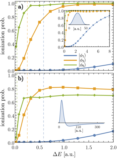
Figure 1: Ionization probability for different initial states by applying HCPs with a temporal function described by $\mathcal{F}_{\rm HCP}^{(1)}(t)$ or $\mathcal{F}_{\rm HCP}^{(2)}(t)$ HCP (Eqs. 8, 9) in dependence on the energy shift $\Delta E_{k}$ ($\Delta E_{k}$ refers to the first half cycle). Vertical lines denote the estimated ionization thresholds.

For the simulations, we used HCPs with a duration 50 a.u. (first half cycle), which were applied to the system in the ground and excited states. Although the electron orbiting times $\tau_{i}$ in these states are considerably shorter than the pulse duration, one observes satisfactory agreement between the position of the steep increase of the ionization probability and the threshold energies. For instance, the probability of ionization at threshold is approximately 32% for the second state. For the 6th state, it is already 42%. In contrast, for the ground state $\tau_{p}\gg\tau_{1}$, so that the Magnus approximation is insufficient, which is highlighted by the negligible ionization probability at the threshold energy.
The HCP application with zero momentum transfer (Fig. 1, right panel) does not qualitatively change the picture of the ionization observed for the ideal HCP. There are, however, critical quantitative differences. First, the system can never be fully ionized due to recombination. Second, different states reach different saturated levels of ionization. Further, at much larger values of the energy transfer, the ionization slowly drops down. Such behavior is anticipated for higher energy states or shorter pulses. In Ref. Wesdorp et al., 2001, it was experimentally shown that the long tails of realistic HCPs start to be significant only when the duration of the whole pulse is in the regime of impulsive kick, i.e., when the orbiting time of the electron is longer. In our one-dimensional calculations, a sizeable effect of the long tail of HCP appears for much longer pulse lengths. Further, we note the clear difference to ionization with two alternating $\delta$-pulses leading to the full ionization of the system at sufficiently large momentum transfer Grozdanov and Jaćimović (2009).
Second finding is the observation of an ionization onset at lower fields by using $\mathcal{F}_{\rm HCP}^{(2)}(t)$ instead of $\mathcal{F}_{\rm HCP}^{(1)}(t)$. For example, at the threshold energy $E_{2}$, one achieves an ionization probability of almost 10% higher for the second state (43% to 52%). This effect was also observed experimentally Wesdorp et al. (2001).

III.2 Off-resonant excitation and ionization with HCP

The application of short electromagnetic pulses of high intensity to an atomic system leads among other effects to above threshold ionization (ATI). Wassaf et al. performed detailed studies of the present one-dimensional model system Wassaf et al. (2003b, a). Their results closely mimicked experimental observations and explained the resonance-like enhancements in ATI spectra. The drawn conclusions on the origin of the effect can be considered complementary to another explanation based on the "channel closing"-hypothesis Popruzhenko et al. (2002); Borca et al. (2002). In the present work, we reproduced the aforementioned spectra, albeit with a different numerical method.

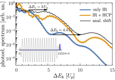
Figure 2: Photoelectron spectrum as a function of the energy of ejected electrons measured in units of the ponderomotive potential ($U_{p}$). The system is excited with a trapezoidal pulse (shown in the inset) with an intensity of $1.12\cdot 10^{14}$ W cm² and $\hbar\omega=1.57$ eV. We compare the ATI spectrum obtained without and with the presence of a HCP with a duration of 50 a.u. applied at the end of the first pulse. The solid black line denotes the hypothetical ATI spectrum obtained by applying the analytical energy shift (cf. Eq. 10).

Furthermore, we study the effects of an additional HCP. The atom is excited with an electromagnetic pulse of 1960 a.u. duration and frequency of 0.0577 a.u., the energy of the photon is typical for Ti:sapphire laser. The pulse comprises 18 optical cycles and has an intensity of $1.12\cdot 10^{14}$ W cm² (Fig. 2, inset). It should be noted that a straightforward application of these equations leads to oscillations in the ATI spectra which can be removed by averaging. We present only averaged spectra noting that several components of these oscillations are discussed in detail in Ref. Wassaf et al. (2003b). The distance between major peaks corresponds to the energy of one photon, while subpeaks signify processes involving excited states.
In our first numerical experiment (Fig. 2), we study the influence of the HCP, which is applied at the end of the few-cycle pulse, on the ATI spectrum. The HCP has a sin² shape with 50 a.u. duration and $E_{0}=2.24\cdot 10^{-2}$ a.u. maximal electric field strength. The HCP is applied at the moment $t=1950$ a.u. so that we find a small interval of time when both pulses intersect. The energy transferred to the system by the HCP ($\Delta E=0.16$ a.u.) is insufficient to ionize the system. However, its influence is prominent. It provides not only the expected energy shift (analytical treatment of this effect is depicted by the black line) of the spectrum but also substantially reduces the electron yield and introduces additional peaks (Fig. 2, cf. orange curve). The first peak with the energy of $0.65U_{p}$ originates from stripping off the electron population from the higher excited states due to the HCP action. This statement is supported by the energy balance ($U_{p}=0.24$ a.u., $q=0.56$ a.u., $\Delta E=0.65U_{p}$). However, the origin of the peak at $3U_{p}$ and the smaller photoelectron yield cannot be inferred from Fig. 2 alone. Hence, we performed a series of calculations where we apply HCPs with different durations ranging from $\tau_{p}=50$ a.u. to $\tau_{p}=1000$ a.u. and a fixed momentum transfer of 0.42 a.u.. We do so while the atom is subjected to the longer laser pulse (Fig. 3).

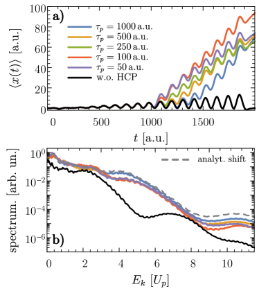
Figure 3: The time-dependent expectation value of the position (left panel) and photoelectron spectrum (right panel) for HCPs of different durations while the momentum transfer of 0.42 a.u. kept fixed. The HCPs are applied to the system at $t=1000$ a.u.. Colored curves correspond to the application of IR laser field with HCP, and the black curve to the case when only the HCP is present. Analytical energy expected shift is indicated by the gray, dashed curve in panel b).

The ATI spectrum depends strongly on the duration of the pulse. Longer pulses have a weaker influence on the electron yield, as shown in Fig. 3 (blue and orange curves). Shorter pulses, reduce significantly the emission of electrons with larger kinetic energies. This effect is more pronounced in the vicinity of the resonant enhancements, in line with the classical description of electron rescattering during ATI, as was originally suggested by Paulus et al. for two-color ATI Paulus et al. (1995).

III.3 Combination of optical vortex and HCP

For the optical vortex propagating along the $z$-axis, the helicity $\sigma$ and carried photonic orbital angular momentum $m$ have the same sign (total angular momentum is $(m+\sigma)\hbar$). Such a structured field is called a parallel class vortex and can be described by a transverse vector potential, so that $\boldsymbol{\nabla}\cdot\boldsymbol{A}(\boldsymbol{r},t)=0$ is valid to an very good approximation Wätzel and Berakdar (2020). The atom is located at the optical axis. In such a case, the vector potential is given in cylindrical coordinates $\boldsymbol{r}=\{\rho,\varphi,z\}$:

$$\boldsymbol{A}(\boldsymbol{r},t)=A_{0}\boldsymbol{e}\left(\frac{\rho}{w_{0}}\right)^{|m|}e^{im\varphi}\Omega(t)e^{-i\omega t}+c.c.,$$ (11)

where $A_{0}$ is the amplitude, $w_{0}$ is the beam waist, $\Omega(t)$ is the temporal envelope and $\boldsymbol{e}_{\sigma}=(\boldsymbol{e}_{\rho}+i\sigma\boldsymbol{e}_{\varphi})\exp(i\sigma\varphi)$ is the circular polarization vector. In the following, we consider the argon atom to be irradiated by the vortex with $\sigma=+1$, $m=+1$, and a photon energy of $\hbar\omega=14.96$ eV (0.55 a.u.). The absorption of one vortex photon is not sufficient to ionize from the ground state, but from higher unoccupied states if they were photo-excited by another pulse. Multi-photon processes are captured by the numerical propagation and result in photoelectron spectra with major peaks separated by $\hbar\omega$.
The results shown in Fig. 4 correspond to a $\sin^{2}$ envelope with a pulse length of 8 optical cycles. The amplitude belongs to a peak electric field of $E_{0}=5$ a.u. at the donut rim (waist $w_{0}=50$ nm) of the vortex. However, since the argon atom is located in the singularity (where $\boldsymbol{A}(\rho=0,t)=0$), the valence shell electron is exposed to a relatively weak electric field. The red curve in Fig. 4 corresponds to the case when only the vortex field is applied, while the black curve belongs a combination of a vortex and HCP pulses. In panel b), we present the $z$-projection of the angular momentum $\langle m\rangle=\langle\Psi(t)|\hat{L}_{z}|\Psi(t)\rangle/\langle\Psi(t)|\Psi(t)\rangle$ attained by the photoelectron in the dependence on the kinetic energy $E_{k}$. With every absorption of a vortex photon (in absence of the HCP), an angular momentum exchange of $2\hbar$ occurs so that at every major peak in the spectrum, see Fig. 4a), $\langle m\rangle$ increases by two. The third peak around $E_{k}=1.8$ a.u. is not very well developed, which can be explained by the low local field amplitude around the singularity. Now let us switch on an attosecond HCP Wu and Meyer-ter Vehn (2012); Xu et al. (2018) described by $\mathcal{F}_{\rm HCP}^{(1)}(t)$ with a duration of $\tau_{p}=100$ as (4.13 a.u.) and $E_{0}=0.05$ a.u. yielding a momentum kick $q=0.103$ a.u. ($\Delta E=0.005$ a.u.). The temporal profiles of both pulses are shown in the inset in Fig. 4a). Relative to the optical vortex (which propagates in $z$-direction), the HCP is directed along the $x$-axis, meaning it acts in the same plane as the vortex vector potential $\boldsymbol{A}(\boldsymbol{r},t)$. Similar to Sec. III.2, the HCP has a clear impact on the photoelectron spectrum and $\langle m\rangle$.

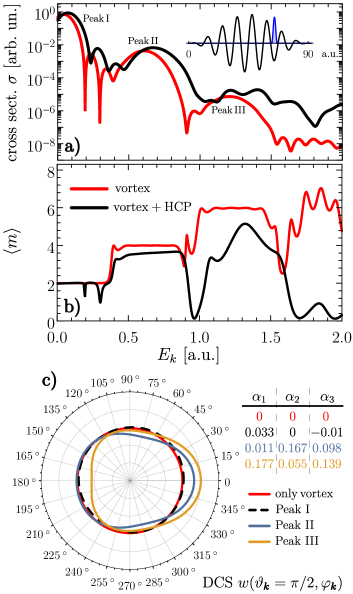
Figure 4: Ionization of the Argon atom using a combination of the optical vortex and the attosecond half-cycle pulse (shown in the inset of panel b). (a) The photoemission cross-section for using only a vortex and the combination. (b) Angular momentum attained by the photoelectron. (c) Angular distribution of the photoelectrons in the polarization plane and the $\beta$ parameters Schmidt (1997) (see main text) for the different major peaks in the photoemission spectrum. The black curve corresponds to applying only the vortex. For clarity, all DCS are normalized to the same total cross section $\sigma$.

On the one hand, the maxima of the cross section are shifted, which can be attributed to the attosecond HCP momentum kick and follows roughly Eq. (10). On the other hand, the photoelectron yield is visibly increased. Further, the attained angular momentum is clearly damped due to the action of the HCP, so that the "stair"-like behavior ($\langle m\rangle$ increases by two for every major peak) does not apply to the combined irradiation of both laser fields. Strong effects can be observed for higher energies $E_{k}>1.5$ a.u., where the effect of the vortex (relative to the HCP) is virtually non-existent. Therefore, also $\langle m\rangle$ is practically zero.
The differential cross section (DCS) has an angular dependence of the two-laser excitation/ionization process. As both electromagnetic fields act in the $x-y$ plane, we study the azimuthal variation of the DCS at $\vartheta_{\boldsymbol{k}}=\pi/2$, which is shown by Fig. 4c). Without the HCP (only the vortex field is present, red curve), the DCS is invariant with respect the azimuthal angle variation which stems from the cylindrical symmetry of the vortex field. In the presence of the HCP, however, the forward-backward symmetry of the photoionization process is broken and the degree of the asymmetry depends on the kinetic energy of the photoelectron. Here, the depicted DCS curves are averaged over the widths of the major peaks in the photoelectron spectrum, shown in Fig. 4a). Observing the photoelectron at a higher (major) peak in the cross section, increases the degree of asymmetry. For a more clear quantification of the symmetry break, we can fit the (peak-averaged) DCS curves to

$$\bar{w}_{p}(\vartheta_{\boldsymbol{k}}=\pi/2,\varphi_{\boldsymbol{k}})\propto 1+\sum_{n}^{3}\alpha_{n}P_{n}(\cos(\varphi_{\boldsymbol{k}})),$$ (12)

where $p$ is the index of the observed major peak, $P_{n}(x)$ are the Legendre polynomials of degree $n$, and $\alpha_{n}$ can be interpreted as the asymmetry parameter for the azimuthal dependency. We note that in comparison to the conventional introduction of asymmetry parameter $\beta$ Taylor (1977); Hemmers et al. (1997); Dixon (2005); Child (2008) (which describes the full solid angle dependency of the DCS), this is a very simple model whose sole purpose is the quantification of the DCS deformation in the azimuthal plane due to the action of the HCP. While $\alpha_{2}$ reflects symmetry between $\varphi_{\boldsymbol{k}}$ and $\varphi_{\boldsymbol{k}}-\pi$, $\alpha_{1}$ and $\alpha_{3}$ quantify asymmetry. We note that in most of the existing literature, the expansion in Eq. (12) refers to the polar angle $\vartheta_{\boldsymbol{k}}$ for $z$-linearly polarized fields. Here, however, both polarization vector point in the azimuthal plane, so that an expansion in the dependence on $\varphi_{\boldsymbol{k}}$ is reasonable.
Applying the vortex field only (without the HCP) yields a cylindrically symmetric DCS for all three ionization peaks. Therefore, all $\alpha_{n}$ are virtually zero. Adding now the HCP causes an asymmetry in the photoelectron’s momentum distribution. Physically, the valence shell electron is now preferentially ejected into the HCP polarization direction ($x>0$). Moreover, this effect is even more pronounced when observing the photoelectron at higher kinetic energies $E_{k}$. This is highlighted by the increased $\alpha$ parameter with odd $n$. As indicated by Fig. 4b), the presence of the HCP is – at least for the first two peaks – not obstructive for the angular momentum transfer to the electron, i.e., $\langle m\rangle$ shows the same trends. Therefore, the application of an HCP has the advantage that we can steer the emission direction of a photoelectron with encapsulated angular momentum.

IV Conclusions

This numerical study shows that the photoelectron spectra produced in an above-threshold-ionization of an atom in an intense laser field can be modified by applications of time-asymmetric pulse that shifts the linear momentum of the electron. The amount of this shift is set by the duration and the peak electron field of the applied pulse. If the laser field is an optical vortex carrying orbital angular momentum, the photoelectrons may attain an electronic angular shift that we can quantify by the expectation value of the orbital angular momentum along with the propagation directions. This orbital angular momentum can be quenched or maintained by applying appropriate time asymmetric pulses.