Huffing, and puffing, and blowing your house in:
Strong stellar winds interaction with a super massive black hole

Abstract

We present analytic and numerical models of a cluster wind flow resulting from the interaction of stellar winds of massive stars, with a super massive black hole (SMBH). We consider the motion of the stars as well as the gravitational force of the SMBH. In the numerical simulations we consider two cases: the first one with the stars is in circular orbits, and the second one with the stars in eccentric orbits around the SMBH. We found that after the system reaches an equilibrium, the circular and elliptical cases are very similar. We found a very good agreement between the analytical and numerical results, not only from our numerical simulations but also from other high resolution numerical calculations. The analytical models are very interesting, since the properties of such complex systems involving strong winds and a massive compact object, can be rapidly inferred without the need of a numerical calculation.

1 Introduction

The volume of a sufficiently evolved stellar cluster is filled by the winds from the cluster stars. The interacting stellar winds produce an inhomogeneous, outwards flow which has been called the “cluster wind”.

This cluster wind was described in terms of a steady, mass loaded flow, analytically by Cantó et al. (2000). In an earlier paper, Chevalier & Clegg (1985) found an equivalent solution for a cluster wind driven by supernova explosions.

The mass loaded cluster wind model was explored in more detail by Silich et al. (2004); Rodríguez-González et al. (2007) and Palous̆ et al. (2013) who studied the effects of different stellar distributions (within the cluster) and radiative energy losses. Falle et al. (2012) used the same “cluster wind solution” to model the flow produced by a group of photoevaporating gas clumps.

Full, 3D gasdynamical simulations of the production of a cluster wind through the interaction of many stellar winds were presented by Raga et al. (2001); Rodríguez-González et al. (2007, 2008); Hueyotl-Zahuantitla et al. (2010); Palous̆ et al. (2013). The related problem of the detonation of a single supernova within a cluster wind was studied by Rodríguez-Ramírez et al. (2014) and Castellanos-Ramírez et al. (2015).

None of these studies considered either the motions of the stars within the cluster nor the effect of the cluster’s gravitational field. This is justified since the velocities of the stars (typically of a few km s^-1) and the escape velocity from cluster are much lower than the stellar wind velocities (of $\sim 10^{3}$ km s^-1).

An interesting case is where the orbital velocities of the stars in a cluster are comparable with the velocity of the stellar winds, for instance if the stellar cluster contains in its center a super massive black hole (SMBH) (or of intermediate mass). In such a cluster the orbital velocities of the stars could be as high as $\sim 10^{4}$ km s^-1.

A clear example of this situation are the stars orbiting the black hole at the centre of the Galaxy (see, e.g., Genzel et al. 2003, Ghez et al. 2005), associated with the Sgr A^∗ radio source.

Yusef-Zadeh et al. (2016) pointed out that the extra kinetic energy of the stellar winds resulting from the rapid stellar motions, can help to explain the high $\sim 4\times 10^{7}$ K temperature of the Galactic centre X-ray emitting bubble (Baganoff et al., 2003; Wang et al., 2013), because the stellar wind velocities (of $\sim 1000$ km s^-1) alone are definitely insufficient to produce the observed temperature.

Inspired by the observations we study cluster wind models for a system of stars that are orbiting around a central, massive black hole. In our models we consider both the motion of the stars and the action of the gravitational force (from the central black hole) on the cluster wind.

Several papers have explored numerical models of cluster winds and a SMBH (Sgr A*) (Rockefeller et al., 2004; Cuadra et al., 2005, 2006; Cuadra, Nayakshin & Martins, 2008; Lützgendorf et al., 2016). Ressler, Quataert & Stone (2018) model the winds from 30 Wolf-Rayet stars that dominate the accetion budget in Sgr A*. They include the radiative cooling, collisional ionization equilibrium,up-to-date stellar mass-loss rates, wind velocities and locations of the closest stars of Sgr A*. Very recently Ressler, Quataert & Stone (2020) performed MHD simulations of Sgr A* and magnetized winds of Wolf-Rayet stars orbiting it. They found a very small impact of magnetic fields in the accretion of material in Sgr A* from Wolf-Rayet stellar winds.

In the present paper we do not take into account magnetic fields. We approach the problem in two ways:

• a generalization of the analytical steady, mass loaded flow solution of Cantó et al. (2000) to include the stellar motions and the gravitational force of the black hole,

• 3D gas-dynamic simulations including the winds from $\sim 100$ orbiting stars for two cases: circular and eccentric orbits.

The analytic models that we develop are similar to the ones of Silich et al. (2008), who also modeled a wind from a cluster with a central SMBH. Our models differ from their results in that we include both the gravitational pull of the SMBH and the motions of the stars. These motions were not included in the analytic model of Silich et al. (2008).

Our analytic models are based on equations similar to the ones of previous papers:

• Quataert (2004) derived the gasdynamic equations for a mass-loaded wind from a cluster with a central, massive compact object, and carried out time-integrations to obtain the steady, critical wind solution,

• Silich et al. (2008) presented analytical considerations and numerical solutions of the steady state version of the same equations,

• Shcherbakov & Baganoff (2010) presented numerical integrations of the cluster wind+central massive object problem including a thermal conduction and a two-temperature description of the flow,

• Yalinevich et al. (2018) studied the same problem as Silich et al. (2008), and presented analytic solutions for different limiting regimes.

The models presented in these papers differ from ours in that they do not include the motion of the stellar wind sources when calculating the energy injected by the stellar winds into the cluster wind.

Our models do not consider radiative cooling for the cluster wind flow (which is appropriate for the Galactic centre cluster).

The paper is organized as follows. In Section 2 we develop the mass loaded wind formalism, obtain solutions and explore different flow parameters. In Section 3 we present a full, 3D gas-dynamic simulation of the cluster wind flow. Finally, we discuss our results in Section 4, and the provide with the conclusions in Section 5.

2 The cluster wind as a steady, mass-loaded flow

2.1 General considerations

We consider a stellar cluster with a central massive object of mass $M_{bh}$. We assume that the stars within the cluster have identical stellar winds, with a mass loss rate ${\dot{M}}_{w}$ and terminal velocity $v_{w}$, and that the production of these winds is not affected by the possible near presence of the massive central object. In addition, we assume that the stars have a uniform distribution (with a number density $n$ of stars per unit volume), inside an outer cluster radius $R_{c}$, and that the cluster has many stars, so that the “cluster wind” (produced by the merging of the winds from the individual stars) can be modeled with a “mass loaded flow” formalism, in which the stellar winds are included as a continuous source of mass and energy. Furthermore, we consider a time-independent configuration of a steady cluster wind flow.

The rate of mass injection (per unit volume and time) is:

$${\dot{m}}=n{\dot{M}}_{w}\,,$$ (1)

which is independent of position in our constant $n$ and ${\dot{M}}_{w}$ cluster.

If the stars are moving in random orbits around the central black hole, the net injection of linear and angular momentum due to the orbital motion of the stellar wind sources is zero. This of course is true only in the limit of a high spatial density of stellar wind sources. For a real case in which the number of cluster stars is not so large, localized regions of organized linear and angular momentum are likely to exist, and they will drive turbulence in the cluster wind. To describe this effect, one has to go beyond the simple, mass-loading formalism which we are using here, and we will therefore assume no net momentum injection from the stellar winds.

In order to calculate the kinetic energy injection from the winds, it is necessary to calculate the mean kinetic energy that results from the superposition of the wind velocity $v_{w}$ and the orbital velocity $v_{o}$ of a cluster star. In a reference frame at rest with respect to the central, massive object, the square of the velocity modulus of the material ejected from the orbiting star is

$$W^{2}(\theta)=(v_{w}\cos\theta+v_{o})^{2}+v_{w}^{2}\sin^{2}\theta\,,$$ (2)

where $\theta$ is the angle measured from the direction of the orbital motion. The mean squared velocity of the ejected material then is:

$$\overline{v^{2}}=\frac{1}{4\pi}\int_{0}^{\pi}W^{2}(\theta)\,2\pi\sin\theta d\theta=v_{w}^{2}+v_{o}^{2}\,,$$ (3)

where $W^{2}(\theta)$ is given by equation (2).

In order to proceed, we make the simplest possible assumption of circular orbits around the central black hole for the cluster stars. Then the orbital velocity $v_{o}$ is

$$v_{o}=\sqrt{\frac{GM_{bh}}{R}}\,,$$ (4)

where $G$ is the gravitational constant, and $R$ the spherical radius. Thus, the rate of wind kinetic energy injection (per unit time and volume) by the stellar winds is:

$${\dot{e}}_{kin}=\frac{n{\dot{M}}_{w}}{2}\left(v_{w}^{2}+\frac{GM_{bh}}{R}\right)\,,$$ (5)

where we have used equations (3) and (4). The stellar winds also introduce gravitational potential energy into the combined cluster wind at a rate:

$${\dot{e}}_{pot}=-n{\dot{M}}_{w}\frac{GM_{bh}}{R}\,.$$ (6)

The mass and energy input rates integrated in a volume out to a radius $R$ are equal to the integral over the $R$-surface of the mass and energy fluxes (which in our spherically symmetric models amounts to multiplying the fluxes by $4\pi R^{2}$). The mass flux is

$$F_{mass}=\rho v\,,$$ (7)

where $\rho$ is the density and $v$ the velocity of the cluster wind. The energy flux is:

$$F_{en}=\rho v\left(\frac{v^{2}}{2}+\frac{\gamma}{\gamma-1}\frac{P}{\rho}-\frac{GM_{bh}}{R}\right)\,,$$ (8)

where $P$ is the gas pressure and $\gamma=c_{p}/c_{v}$ is the ratio of specific heats ($=5/3$ for a monoatomic gas). The equations resulting from equating the volume integrals of the mass (equation 1) and energy (equations 5-6) source terms with the surface integrals of the corresponding fluxes (equations 7-8) are given in the following section.

2.2 The flow equations

The resulting mass conservation equation is:

$$4\pi R^{2}\rho v=\frac{4\pi}{3}R^{3}n{\dot{M}}_{w}\,,$$ (9)

and the energy conservation gives:

$$4\pi R^{2}\rho v\left(\frac{v^{2}}{2}+\frac{\gamma}{\gamma-1}\frac{P}{\rho}-\frac{GM_{bh}}{R}\right)=$$

$$\frac{2\pi n\dot{M}_{w}}{3}\left(R^{3}v_{w}^{2}-\frac{3}{2}GM_{bh}R^{2}\right)\ \mbox{ ,}$$ (10)

where the right hand side of equation 10 is the result of integrating ${\dot{e}}_{kin}$ + ${\dot{e}}_{pot}$ over the volume.

Also, we have to consider an equation of motion of the form:

$$\rho v\frac{dv}{dR}=-\frac{dP}{dR}-n{\dot{M}}_{w}v-\rho\frac{GM_{bh}}{R^{2}}\,,$$ (11)

where the three terms on the right hand side are the pressure gradient force, the drag force necessary for incorporating the stellar winds into the cluster wind flow and the gravitational attraction of the central black hole. Note that we have ignored the gravity force of the stars.

Equations (9-11) are valid within the cluster radius, i.e., for $R\leq R_{c}$. The flow equations for $R>R_{c}$ are obtained by setting $R=R_{c}$ in the right-hand sides of equations (9) and (10), and $n=0$ in the right-hand-side of equation (11).

Combining equations (9-10) we obtain

$$\rho=\frac{n{\dot{M}}_{w}R}{3v}\,,$$ (12)

$$c_{s}^{2}=\frac{\gamma-1}{2}\left(v_{w}^{2}-v^{2}+\frac{GM_{bh}}{2R}\right)\,,$$ (13)

where $c_{s}=\sqrt{\gamma P/\rho}$ is the sound speed. Using these two relations, we can then turn the equation of motion (equation 11) into a differential equation involving only the velocity $v$ of the gas:

$$\frac{dv}{dR}=\frac{2v}{R}\frac{(1+5\gamma)v^{2}+(\gamma-1)v_{w}^{2}+2\gamma GM_{bh}/R}{2(\gamma-1)v_{w}^{2}-2(\gamma+1)v^{2}+(\gamma-1)GM_{bh}/R}\,.$$ (14)

An integration of equation (14) gives the velocity of the cluster wind as a function of radius $R$, and substituting this solution into equations (12) and (13) we obtain the spatial dependence of the density and sound speed (respectively) of the wind in the $R\leq R_{c}$ region.

Outside the edge of the cluster (for $R>R_{c}$, see the text following equation 11), the density, sound speed and velocity of the cluster wind are given by:

$$\rho=\frac{n{\dot{M}}_{w}R_{c}^{3}}{3R^{2}v}\,,$$ (15)

$$c_{s}^{2}=\frac{\gamma-1}{2}\left[v_{w}^{2}-v^{2}+GM_{bh}\left(\frac{2}{R}-\frac{3}{2R_{c}}\right)\right]\,,$$ (16)

where $c_{s}=\sqrt{\gamma P/\rho}$ is the sound speed. Using these two relations (and setting $n=0$ in equation 11), we can then turn the equation of motion into a differential equation involving only the velocity $v$ of the gas:

$$\frac{dv}{dR}=\frac{2v}{R}\times$$

$$\frac{(\gamma-1)(v_{w}^{2}-v^{2})+GM_{bh}\left[(2\gamma-3)/R-3(\gamma-1)/(2R_{c})\right]}{(\gamma+1)v^{2}-(\gamma-1)v_{w}^{2}+(\gamma-1)GM_{bh}[3/(2R_{c})-2/R]}\,.$$ (17)

2.3 The dimensionless flow equations

We use the radius at which the circular orbital velocity is equal to the velocity of the stellar winds

$$R_{0}=\frac{GM_{bh}}{v_{w}^{2}}\,,$$ (18)

and $v_{w}$ to define a dimensionless radius $r=R/R_{0}$, and velocity $u=v/v_{w}$ . The dimensionless radius of the cluster is then $r_{c}=R_{c}/R_{0}$. In terms of these dimensionless variables, the flow equations for $r\leq r_{c}$ (see equations 12-17) become:

$$\frac{\rho}{\rho_{0}}=\frac{r}{u}\,,$$ (19)

$$\left(\frac{c_{s}}{v_{w}}\right)^{2}=\frac{\gamma-1}{2}\left(1-u^{2}+\frac{1}{2r}\right)\,,$$ (20)

$$\frac{du}{dr}=\frac{2u}{r}\frac{(1+5\gamma)u^{2}+\gamma-1+2\gamma/r}{2(\gamma-1)-2(\gamma+1)u^{2}+(\gamma-1)/r}\,,$$ (21)

where $\rho_{0}=n{\dot{M}}_{w}GM_{bh}/(3v_{w}^{3})$ in equation (19).

For $r>r_{c}$ (outside the cluster radius see equations 15-17), the dimensionless flow equations can be written as:

$$\frac{\rho}{\rho_{0}}=\frac{r_{c}^{3}}{r^{2}u}\,,$$ (22)

$$\left(\frac{c_{s}}{v_{w}}\right)^{2}=\frac{\gamma-1}{2}\left(1-u^{2}+\frac{2}{r}-\frac{3}{2r_{c}}\right)\,,$$ (23)

$$\frac{du}{dr}=\frac{2u}{r}\frac{(\gamma-1)(1-u^{2})+(2\gamma-3)/r-3(\gamma-1)/(2r_{c})}{(\gamma+1)u^{2}-(\gamma-1)+(\gamma-1)[3/(2r_{c})-2/r]}\,.$$ (24)

Figure 1: Radial profiles of density (top row), velocity (middle row, and sound speed (bottom row). The solutions were obtained for different cluster radii: $r_{c}=1.55$ (left column), $r_{c}=2.0$ (middle column), and $r_{c}=5.0$ (right column).

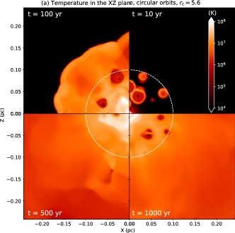
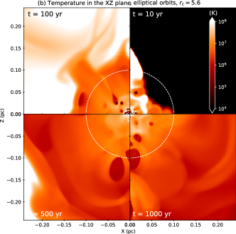
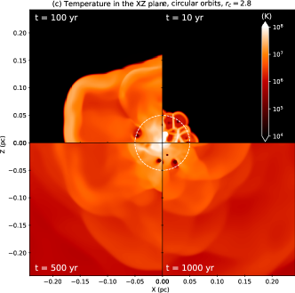
Figure 2: We show the evolution of the temperature in the Y-midplane for four integration times in the simulation: t=10 (upper-right panels), 100 (upper-left panels), 500 (lower-left panels) and 1000 yr (lower-right panels). The white circle shows the size of the stellar cluster with radius $R_{c}$. The units of the color bars are given in K. The Figure labeled “(a)”, shows the temperature evolution for the circular orbit case and $r_{c}=5.6$, the Figure labeled “(b)”, shows the evolution of the temperature for the elliptic orbit case and $r_{c}=5.6$, and the Figure labeled “(c)” shows the evolution of the circular orbit case and $r_{c}=2.8$.

2.4 Analytical considerations

An inspection of equation (21) shows that for a cluster with a finite velocity close to the origin (e.g. near the location of the massive object at the centre of the cluster) the $2\gamma/r$ and $(\gamma-1)/r$ dominates over the other terms in the numerator and denominator (respectively). Neglecting these other terms, for $r\ll 1$ we then have:

$$\frac{du}{dr}=\frac{4\gamma u}{(\gamma-1)r}\,,$$ (25)

which has the solution

$$u=\left(Ar\right)^{4\gamma/(\gamma-1)}\,,$$ (26)

where $A$ is an integration constant. We should note that for $\gamma=5/3$, the exponent in equation (26) has a value of 10.

If for larger $r$ the velocity $u$ continues to increase, $du/dr$ will eventually diverge. This divergence occurs at the point in which the denominator of equation (21) is equal to zero. From this condition, we obtain the relation:

$$u_{d}^{2}=\frac{\gamma-1}{\gamma+1}\left(1+\frac{1}{2r_{d}}\right)\,,$$ (27)

where $u_{d}$ is the (dimensionless) cluster wind velocity at the radius $r_{d}$ at which $du/dr$ diverges. Substituting equation (27) into equation (20), we see that $c_{s}/v_{w}=u_{d}$ at $r=r_{d}$. Therefore, at the point $r_{d}$ in which $du/dr$ diverges, the flow is sonic.

Now, if we look at the $r>r_{c}$ solution (equations 22-24), we see that for $r=r_{c}$ the condition for a divergence of $du/dr$ gives

$$u_{c}^{2}=\frac{\gamma-1}{\gamma+1}\left(1+\frac{1}{2r_{c}}\right)\,.$$ (28)

Therefore, if for the inner ($r\leq r_{c}$) solution we choose a radius $r_{d}=r_{c}$ (for $du/dr$ divergence), we the have a continuous transition to the outer ($r>r_{c}$) solution. This matching between the inner and outer solutions with a sonic point at $r=r_{c}$ is equivalent to the one of the “classical” cluster wind solution (i.e., with no gravity), see, e.g. Cantó et al. (2000).

We should point out that in principle, the inner solution could end at a cluster radius $r_{c}<r_{d}$, so that $du/dr$ does not diverge within the cluster. However, this would produce a subsonic velocity at $r_{c}$ (see equation 27 and the text following this equation). The $r>r_{c}$ solution (see equation 24) would then have a subsonic initial condition (at $r=r_{c}$). However, it is a well known result that an adiabatic, spherical flow does not have a sonic transition (see, e.g., the book of Lamers & Casinelli 1999), and the flow will never reach supersonic velocities.

The fact that the fluid has an effective $\gamma<5/3$ in the classical Spitzer isothermal wind (for a single star) is due to the very efficient thermal conduction that is able to maintain a close to isothermal flow. For the physical conditions of the interaction of several winds, the thermal conduction is not as efficient, and thus an adiabatic treatment is more adequate.

Therefore, the only possibility left is to have the critical point of the full, inner+outer solution coinciding with the cluster radius. This result does not hold for an isothermal flow, or for a wind with thermal conduction, in which one can in principle have the sonic point within the outer (and possibly also within the inner) solution.

Another interesting point that can be made through an inspection of the flow equations is as follows. For $r\to\infty$ the wind will reach a constant, terminal velocity. Therefore, $du/dr\to 0$ for $r\to\infty$. Looking at the numerator of equation (24) we see that $du/dr\to 0$ implies that we either have $u\to 0$ (this would be a “stalled wind” solution) or that

$$u^{2}\to u_{\infty}^{2}=1-\frac{3}{2r_{c}}\,.$$ (29)

Therefore, for $r_{c}>3/2$ we will have the terminal wind velocity given by equation (29). Using equations (4) and (18, and noting that $r_{c}=R_{c}/R_{0}$, this condition can be written as $v_{w}>\sqrt{3/2}v_{o}(R_{c})$, where $v_{o}(R_{c})$ is the circular orbital velocity at the outer boundary of the cluster. As will be discussed in the following section, there are no full cluster wind solutions when this condition is not satisfied.

2.5 Flow solutions

The inner flow ($r\leq r_{c}$, within the cluster) can be straightforwardly obtained by numerically integrating equation (21), starting with an off-center $(u,r)$ initial condition found through the $r\ll 1$ flow solution of equation (26) with an appropriately chosen value for the $A$ integration constant (this choice of $A$ is done by trying different values until the desired cluster radius $r_{c}$ is obtained). The numerical integration is continued until the flow velocity $u(r)$ becomes less or equal than the velocity expected for the cluster edge (the velocity $u_{c}$ of equation 28, computed at $r_{c}=r$).

When this condition is met, we have arrived at the edge of the cluster, and therefore switch to an integration of the outer flow equation (24), starting at the current $(u,r)=(u_{c},r_{c})$ values.

Alternatively, one can use the analytic integral:

$$f(r,u)=u^{2}+\frac{2u_{c}^{\gamma+1}}{(\gamma-1)u^{\gamma-1}}\left(\frac{r_{c}}{r}\right)^{2(\gamma-1)}-\frac{2}{r}+\frac{2}{r_{c}}-\frac{\gamma+1}{\gamma-1}u_{c}^{2}=0\,.$$ (30)

This solution can be straightforwardly obtained by noting that the outer flow follows an adiabat (i.e., that $c_{s}^{2}\propto\rho^{\gamma-1}$), and combining this condition with equations (9) and (10). In order to obtain $u(r)$, we fix values for $r$ (starting at $r=r_{c}$, where the outer flow starts) and numerically find the values of $u$ for which $f(r,u)=0$.

Interestingly, for $r_{c}\leq 3/2$ equation (30) has no zeroes for $r>r_{c}$. Therefore, in order to have a steady cluster wind the $r_{c}>3/2$ condition has to be met (see also the discussion following equation 29). For $r_{c}>3/2$, for all radii $r>r_{c}$ there are two values of $u$ for which equation (30) has zeroes: one of them supersonic (the wind solution) and the other wind subsonic (a “stalled wind” solution). The supersonic $u(r)$ solution coincides with the numerical integration of the outer wind differential equation (equation 24) described above.

In Figure 1 we show the radial structure of the flow velocity, sound speed and density obtained for clusters with $r_{c}=1.55$, 2 and 5 (for a flow with $\gamma=5/3$). For the clusters with $r_{c}=1.55$ and 2 we find that the flow velocity initially grows with $r$, reaches a peak (outside the cluster radius) and then decreases monotonically to attain the asymptotic value given by equation (29). The $r_{c}=5$ cluster has a monotonically increasing $u(r)$ (also converging at large radius to the appropriate asymptotic value).

The sound speed has a divergence at the origin, followed by a sharp decrease which produces a peak extending to $r\sim 1$ (a radius $R\sim R_{0}$, see equation 18). The sound speed then has a plateau (with a sound speed $c_{s}\sim 0.6v_{w}$) extending out to the cluster radius $R_{c}$, and a monotonic decrease with $R$ outside the cluster. The density is a monotonically decreasing function of radius, with a sharper decrease close to the cluster radius (see Figure 1).

We should point out an important difference between our cluster wind solutions and the ones of Silich et al. (2008). These authors find that in order to obtain an outflowing cluster wind, they need to have an inner region in which the flow is directed inwards, accreting onto the SMBH. Quataert (2004) found the same result through an appropriate integration of the time-dependent equations.

Our model differs from the ones of Silich et al. (2008) and Quataert (2004) because it includes the effect of the orbital motion of the stars in the stellar wind energy equation, see our equations 3-5. Because of this difference, we do obtain an outwards directed wind at all radii, provided that the condition $r_{c}=R_{c}/R_{0}>3/2$ is met (see equation 29).

Our equations do not appropriate model the region close to the central BH, i. e. we do not include accretion into the SMBH. However, in this inner region, an infall into the central object is unavoidable.

3 Numerical simulations setup

3.1 The code: guacho + N-body

We carried out 3D-grid hydrodynamic simulations with the guacho code (Esquivel et al., 2009; Esquivel & Raga, 2013). The code solves the ideal hydrodynamic equations in a uniform Cartesian grid with a second-order Godunov method with an approximate Riemann solver (in this case we use the HLLC solver, Toro E. F. 1999), and a linear reconstruction of the primitive variables using a minmod slope limiter to ensure stability. We assume a gas of pure hydrogen, along with the gasdynamic equations we solve a rate equation for neutral hydrogen of the form

$$\frac{\partial n_{HI}}{\partial t}+\nabla(n_{HI}\mathbf{u})=n_{e}n_{HII}\alpha(t)-n_{HI}n_{HII}c(t)\mbox{ ,}$$ (31)

where $n_{HI}$ is the neutral hydrogen density, $n_{HII}$ is the ionized hydrogen density, and $n_{e}$ is the electron density. In this equation we denote u as the flow velocity, $\alpha(t)$ is the recombination (case B) coefficient, and $c(t)$ is the collisional ionization coefficient. The energy equation and the hydrogen continuity equation are integrated forward in time, without the source terms in the hydrodynamic timestep. Instead, the source terms are added in a semi-implicit timestep with which the ionization fraction is updated. We do not include cooling since the cooling times at the temperatures we are working with, are much larger than the evolution time of the simulation.

In order to include the effects of the stellar orbits in the calculation we coupled an N-Body module to the guacho code. The N-body module is a version of the Varone code (Lora et al., 2009). Since we are dealing with a small number of particles/stars ($N=100$), we are able to compute all the gravitational interactions between them, and thus we use a direct variant of the Varone code/module. The N-body module updates the positions of the wind sources at every timestep of the hydrodynamic code, which also adds the orbital velocity to the wind velocity.

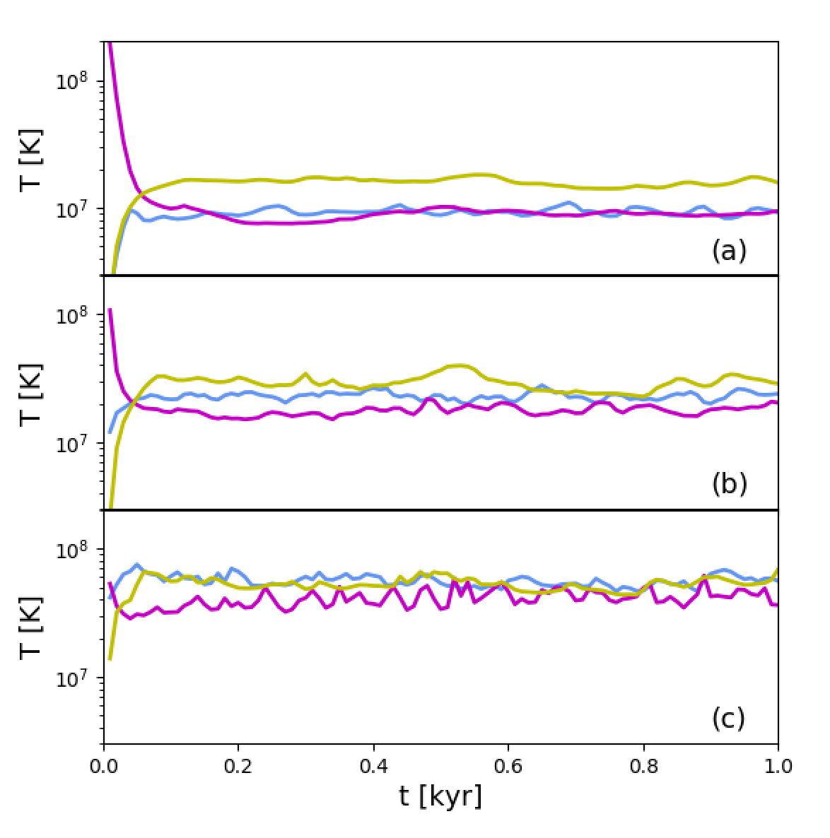
Figure 3: In this Figure we show the average of the temperature inside a sphere of a different radii. The blue lines correspond to the circular model, the magenta lines correspond to the elliptical model, and the yellow lines correspond to the small circular model. In panel $a$ we show the average temperature inside a sphere of radius $R\simeq 0.1$ pc (which is equivalent to $r_{c}$ in the circular and elliptical models). In panel $b$ we show the average temperature inside a sphere of radius $R\simeq 0.05$ pc (which is equivalent to $r_{c}/2$ for the circular and elliptical models). In panel $c$ we show the average temperature inside a sphere of radius $R\simeq 0.025$ pc (which is equivalent to $r_{c}/5$ for the circular and elliptical models).

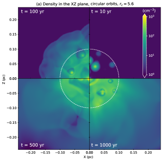
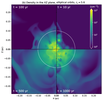
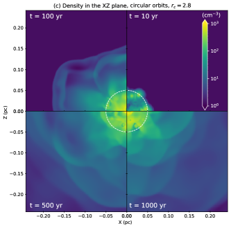
Figure 4: We show the evolution of the density in the Y-midplane for four integration times in the simulation; t=10 (upper-right panels), 100 (upper-left panels), 500 (lower-left panels) and 1000 yr (lower-right panels). The white circle shows the size of the stellar cluster with radius $R_{c}$. The units of the color bar are given in particles cm^-3. The Figure labeled “(a)”, shows the density evolution for the circular orbit case and $r_{c}=5.6$, the Figure labeled “(b)” shows the evolution of the density for the elliptic orbit case and $r_{c}=5.6$, and the Figure labeled “(c)” shows the evolution for the circular orbit case and $r_{c}=2.8$.

3.2 Cluster+SMBH initial conditions

We model a star cluster containing $100$ stars. The computational domain has a physical size of $1.5\times 10^{18}\times 1.5\times 10^{18}\times 1.5\times 10^{18}$ cm ($0.5\times 0.5\times 0.5$ pc) along the $x$-,$y$-, and $z$-axes, which is resolved with a uniform Cartesian grid of 600$\times$600$\times$600 cells.

We impose an isotropic wind for each one of these stars. The stellar winds are imposed to be fully ionized, with a mass loss rate of $\dot{M}=1\times 10^{-6}$ M_⊙/yr. The temperature associated to the star-winds is $T_{wind}=1\times 10^{5}$ K, and the velocity of the stellar wind is $v_{wind}=1\times 10^{8}$ cm/s. The star-wind is centered at each star position within a radius $r_{wind}=1\times 10^{16}$ cm. The outer boundary condition on the surface of these spheres is an outward flowing wind. In this work we do not impose an accreting flow into the black hole. The region where the wind sources are injected is significantly larger than the stellar radius. Therefore, in their orbital motion wind sources occasionally overlap, when this occurs we superimpose the winds of the overlapping sources.

We add a massive particle in the cluster’s center, with a mass $M_{BH}=4\times 10^{6}$ M_⊙ mimicking a SMBH with a mass similar to the one of the SMBH in the center of the Galaxy.

We generate the initial positions and velocities of the $N$-stars considering the mass of the SMBH in the center of the star cluster.

The initial position and orientation of the stars orbits are set randomly within a radius $R_{c}$. For the initial position we draw three random numbers ($x,~{}y,~{}z$) from a uniform distribution between $-R_{c}$ and $R_{c}$, if the position with respect to the center ($r_{*}=\sqrt{x^{2}+y^{2}+z^{2}}$) is larger than $R_{c}$ we discard the random numbers and repeat the procedure until the $N$ stars are placed. We constructed three distributions, two with $R_{c}=3\times 10^{17}~{}\mathrm{cm}$ (corresponding to a dimensionless $r_{c}=R_{c}/R_{0}=5.6$) and one with $R_{c}=1.5\times 10^{17}~{}\mathrm{cm}$ ($r_{c}=2.8$).

For the initial velocities of the stars, once the positions of each of the stars are computed, we calculated the circular velocity of each star considering only the mass of the SMBH ($v_{c,*}=(GM_{BH}/r_{*})^{1/2}$). Then, we chose a random number between zero and 1, and multiply it by the circular velocity at $r_{*}$, for each of the stars. As a result we have random eccentricities of the orbits of the stars.

For the orbital velocities, we built three different cases: in the first two cases we impose a circular orbit to each of the stars in the cluster. To do this we compute the magnitude of the circular velocity at the initial position of each star and we add this velocity, projected onto a random orientation in the plane that is perpendicular to the radial position vector. We ran two models with circular orbits, one with $r_{c}=5.6$ and the second one with $r_{c}=2.8$. In the third model we impose eccentric orbits for the stars in the cluster for a distribution with $r_{c}=5.6$. The mass of each of the stars was set to $M_{*}=1$ M_⊙ for both circular and eccentric orbit cases. The environment is initially at rest, and consists of neutral hydrogen, with a density $\rho_{env}=2.16\times 10^{-24}$ g cm^-3 and a temperature $T_{env}=1\times 10^{4}$ K.

4 Results

We allowed the models to run from the initial conditions described in 3.2 to an evolutionary time $t=1$ kyr, for our initial circular and eccentric orbit cases.

In Figure 2 we show the time evolution of the Y-midplane temperature for four integration times: $10$, $100$, $500$ and $1000$ yr. In (a) we show the case where the orbits are circular with $r_{c}=5.6$, in (b) the case where the orbits are eccentric with $r_{c}=5.6$, and in (c) the case with circular orbits and $r_{c}=2.8$. We show the radius of the cluster, $R_{c}$, as a white circle. We observe that at an integration time $t=10$ yr, almost all of the gas inside the cluster has raised its temperature to at least $\sim 10^{7}$ K. In the eccentric case (Figure 2b) the temperature is somewhat higher.

In order to study quantitatively how the temperature increases inside the star cluster radius of the circular and elliptical case ($R_{c}=3\times 10^{17}$ cm) as time evolves, we computed the average temperature taking into account each computational cell inside this radius, and repeat the procedure for all the snapshots in our simulation. In Figure 3 we plot the temperature as a function of the integration time within a radius $R\simeq 0.1$ pc (panel $a$), $R\simeq 0.05$ pc (panel $b$), and $R\simeq 0.025$ pc (panel $c$). The color code in 3 is the same in the three panels: the color blue represents the circular case (with $R_{c}=3\times 10^{17}$ cm), the magenta color represents the elliptical case (with $R_{c}=3\times 10^{17}$ cm), and the yellow color represents the small circular case (with $R_{c}=1.5\times 10^{17}$ cm).

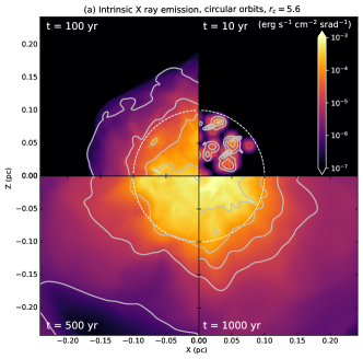
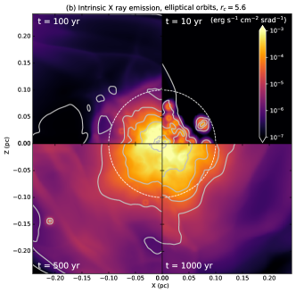
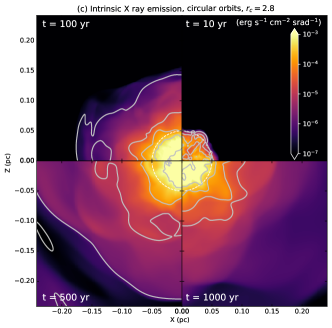
Figure 5: We show the evolution of the X-ray emission in the Y-plane for four integration times in the simulation; t=10 (upper-right panels), 100 (upper-left panels), 500 (lower-left panels) and 1000 yr (lower-right panels). The color palette shows the soft X-ray emission at $0.2$ to $2$ keV. The six white contours show the hard X-ray emission at $2-10$ keV, logarithmically spaced from $10^{-7}$ to $10^{-3}$ erg s^-1 cm^-2 srad^-1.

In the circular orbit case, the average temperature value over all evolution times, inside $R\simeq 0.1$ pc is $0.91\times 10^{7}$ K. The average temperature value inside a radius $R\simeq 0.05$ pc is $2.28\times 10^{7}$ K, and the temperature in the inner part of the cluster (inside a radius $R=\simeq 0.025$ pc) averaged over all times is $5.62\times 10^{7}$ K.

In the elliptic case, the average of the temperature over all times, inside $R\simeq 0.1$ pc is $1.18\times 10^{7}$ K. The temperature averaged over all times inside $R\simeq 0.05$ pc is $1.89\times 10^{7}$ K, and the temperature in the inner part of the cluster (inside a radius $R\simeq 0.025$ pc) is $4.09\times 10^{7}$ K.

In the small circular orbit case, the average of the temperature over all times, inside $R\simeq 0.1$ pc is $1.55\times 10^{7}$ K. The temperature averaged over all times inside $R\simeq 0.05$ pc is $2.85\times 10^{7}$ K, and the temperature in the inner part of the cluster (inside a radius $R\simeq 0.025$ pc) is $5.28\times 10^{7}$ K.

In order to compare the temperature averaged inside $R\simeq 0.025$ pc (panel $c$ in Figure 3) for the circular and elliptical models, we define the ratio $\aries_{e,c}$ as

$$\aries_{e,c}=\left|1-\frac{T_{e,c}}{T_{c,c}}\right|=0.27\mbox{ .}$$ (32)

Where $T_{e,c}$ is the average temperature in the elliptical model, and $T_{c,c}$ is the average temperature in the circular model. The sub-index $c$ refers to the case where the temperature is averaged inside $r\simeq 0.025$. The difference of having elliptical orbits instead of circular orbits in the cluster, gives as a result a decrease in the averaged temperature. That is, when the stars in the cluster have circular orbits, the energy produced from the colliding stellar winds is higher than in the elliptical case.

In the same way as in Equation 33, we define $\aries_{sc,c}$ as

$$\aries_{sc,c}=\left|1-\frac{T_{sc,c}}{T_{c,c}}\right|=0.06\mbox{ .}$$ (33)

In the latter equation $T_{sc,c}$ corresponds to the average temperature value in the small circular orbit model. The behaviour of the small circular and the circular models is very similar.

In an analogous way we computed $\aries_{e,a}=0.3$, $\aries_{sc,a}=0.7$, $\aries_{e,b}=0.17$, and $\aries_{sc,b}=0.25$. Where the sub-index $a$ and $b$ corresponds to the temperature averaged inside a radius $r\simeq 0.05$ and $r\simeq 0.1$, respectively. The net effect when considering elliptical orbits over circular orbits (for all radii analysed) is to decrease the average temperature. The net effect of reducing the size of the cluster radius a factor two, is to increase the temperature, a factor $1.25$ when considering the average temperature inside $R\simeq 0.05$ pc, and a factor $1.7$ when considering the average temperature inside $R\simeq 0.1$ pc.

In Figure 4 we show the time evolution of the Y-midplane number density ($\mathrm{cm}^{-3}$) in the same layout as in Figure 2. In panels (a) and (c) we show the case where the orbits are circular ($r_{c}=5.6$ and $~{}2.8$, respectively), and in panel (b) the case where the orbits are eccentric ($r_{c}=5.6$). We also show the radius of the cluster as a white circle.

In Figure 4 we can see that in both circular and eccentric orbits models a common cluster wind is formed, reaching a quasi stationary state somewhere between $100$ and $500~{}\mathrm{yr}$ of evolution.

With the results of the simulations (density and temperature stratifications) it is possible to estimate the intrinsic X-ray emission from the cluster + SMBH system. For this purpose we compute the X-ray emissivity in two energy bands: one from $0.2$ to $2~{}\mathrm{Kev}$ (soft X-rays), and one from $2$ to $10~{}\mathrm{Kev}$ (hard X-rays). We use the chianti atomic database and its software (Dere et al., 1997, 2019) and assume that the gas is in coronal equilibrium, and that the emission is in the low-density regime (e.g. the emissivity proportional to the square of the density). The emission coefficient is then integrated taking the y-coordinate as the line of sight. We show the resulting emission maps in Figure 5.

We can see that there is an extended emission in the soft X-ray band that is more concentrated towards the center of the cluster but fills the entire domain. At the same time there is a significant emission in hard X-rays, which occurs mostly in the regions where the individual winds interact.

As the common wind forms, the overall X-ray luminosity increases with time and reaches a quasi-steady value after $\sim 500~{}\mathrm{yr}$. The average soft X-ray intrinsic luminosity value after the initial transient is ${7.8\times 10^{34}~{}\mathrm{erg~{}s^{-1}}}$ for the model with circular orbits and $r_{c}=5.66$, ${6.9\times 10^{34}~{}\mathrm{erg~{}s^{-1}}}$ for the one with elliptical orbits and $r_{c}=5.6$, and ${9.2\times 10^{34}~{}\mathrm{erg~{}s^{-1}}}$ for the model with circular orbits and $r_{c}=2.8$. For the hard X-ray intrinsic luminosities the values are ${3.6\times 10^{34}~{}\mathrm{erg~{}s^{-1}}}$ (circular orbits with $r_{c}=5.6$), ${2.3\times 10^{34}~{}\mathrm{erg~{}s^{-1}}}$ (elliptical orbits with $r_{c}=5.6$), and ${2.9\times 10^{34}~{}\mathrm{erg~{}s^{-1}}}$ (circular orbits with $r_{c}=2.8$).

4.1 The analytic and numerical model compared

As can be seen in Figure 6, the temperature reaches a stationary state after $\sim 0.5$ kyr. When the system has reached equilibrium, the numerical results can be compared with the analytical model described in Section 2.

Figure 6 show the velocity (a), the density (b), the temperature (c), and the sound speed (d) as a function of the distance to the center of the star cluster (averaged over all directions) at the end of our simulation ($1$ kyr) for the two models with $r_{c}=5.6$. The solid blue line indicates the case where the stars are set in circular orbits, and the dashed purple line shows the results for the elliptical orbit case (all panels in Figure 6 have the same color code). It is very clear from Figure 6 that at this integration time, the net effect of stars orbiting in either circular or elliptic orbits is almost indistinguishable. Only a small deviation is seen for the velocity (panel a) in the central regions of the stellar cluster. The black lines in each panel of Figure 6 show the analytical model derived in Section 2. One difference between the analytical model and the simulations is the lack of a sharp transition at $r_{c}$ in the latter. This can be attributed to the finite number of stars which make the boundary of the cluster not as sharply defined. In fact, for the case with elliptical orbits in which the radius of the cluster is slightly varying with time produces smoother radial profiles (see for instance the velocity profile). In Figure 7 we show the comparison between the analytical model and the radial profiles resulting from the model with circular orbits and a smaller cluster radius ($r_{c}=2.8$). In this case we see also a satisfactory agreement between the analytical model and the simulation at distances $r>r_{c}$, except for the case of the velocity.

We obtain a very good agreement between the analytic and numerical approach. The agreement is specially good outside the cluster radius, which is shown as a vertical black lines in Figures 6 and 7. Inside the cluster radius the agreement between the two calculations is quite good as well, except for the velocity profile (panel a).

The difference between the analytic cluster wind velocity and the results from our simulation appears to be the result of the fact that the mean outflow velocity (computed from the numerical simulations) is strongly affected by the velocities of the individual stellar winds (while the analytic model only describes a flow made of the combined winds from all of the stars). This effect is clearly less important outside the initial stellar cluster radius (where there are basically no stars).

4.2 Comparison with previous studies

As we mentioned before, Ressler, Quataert & Stone (2018) studied the accretion from strong stellar winds into the SMBH (Sgr A^∗) in the the center of the Galaxy. They modeled the accretion flow generated by 30 Wolf-Rayet stars orbiting Sgr A^∗ (with an inner boundary of $r_{in}=6\times 10^{-5}$ pc). They adopted a mass for the SMBH of $M_{BH}=4.3\times 10^{6}$ M_⊙. The mass loss rate and the velocities of each of the stellar winds were taken from the observational data of Cuadra, Nayakshin & Martins (2008).

We calculated the average mass loss rate and velocity from Cuadra, Nayakshin & Martins (2008), and set the mass of the SMBH to $4.3\times 10^{6}$ M_⊙. With those parameters we could build an analytical approximation following Section 2. In Figure 8 we show the results of Ressler, Quataert & Stone (2018) (their Figure $18$) and compare it to our analytical results. The value of the dimensionless cluster radius for the analytical model is $r_{c}\simeq 11.9$, which corresponds to $R_{c}\simeq 0.22~{}\mathrm{pc}$, and it is indicated by the vertical gray line in Figure 8. The solid lines in Figure 8 correspond to Ressler, Quataert & Stone’s 2018 data and the dashed line correspond to our analytic results. In black we show the density with units $M_{\odot}/\mathrm{pc}^{3}$, the radial velocity is shown in red (with units $\mathrm{pc/kyr}$), and the sound speed is shown in blue (with units $\mathrm{pc/kyr}$), all of which are shown as a function of the distance to the center of Sgr A^∗.

It is very encouraging to obtain a good agreement between Ressler, Quataert & Stone’s 2018 results and our analytical approach. This is a second test which validates the analytical approach and guarantees that this approach can be used to infer some of the properties of the flow generated from strong stellar winds orbiting a massive compact object.

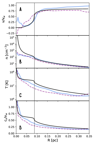
Figure 6: In this Figure we show at an integration time t=1 kyr the velocity normalized by the wind velocity ($1000~{}\mathrm{km\,s^{-1}}$, A), the number density (B), the temperature (C), and the sound speed normalised by the wind velocity (D) averaged over all directions, as a function of radius. The blue solid lines in all panels show the circular orbit case, the purple dashed lines shows the elliptical orbit case, and the black line show the analytical solution. The black vertical line shows the value of R=$R_{c}$, the star cluster radius.

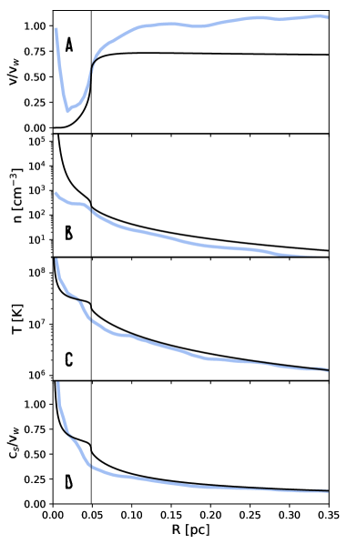
Figure 7: Same as Figure 6 but for the model with circular orbits and $r_{c}=2.8$.

5 Conclusions

In this work we studied for the first time an analytical approximation of a system consisting of a cluster of stars (where all stars present strong winds), orbiting around a massive particle (mimicking a SMBH). In order to validate the analytical model, we run 3D HD numerical simulations of a cluster of stars where each of the stars have a strong associated wind, and are orbiting a massive object in circular and elliptical orbits.

We set all stars with the same parameters of velocity, density, temperature and wind mass-loss rate. We studied three different cases for the orbits of the stars: the first two cases with stars in circular orbits around a SMBH with a mass of $4\times 10^{6}$ M_⊙ and different cluster radius, and a third case where the star orbits are elliptical. We let our numerical simulation run from the initial conditions (described in Section 3.2) to an integration time of $1$ kyr.

We found that after the system has reached a quasi-stationary state (after $\sim 0.5$ kyr) both orbital cases (circular and elliptical) behave virtually the same. We only observe a small deviation between both orbital cases in the velocity profile. In the top panel of Figure 6 it can be seen that the magnitude of the velocity profile inside the cluster is greater for the elliptical case (purple dashed line). We can explain this discrepancy since the elliptical orbital velocities are greater when the stars approach the central region of the cluster where the SMBH is located, thus having overall a greater contribution to the average velocity. Still the difference between the radial velocity profiles is rather small. A very important conclusion in this work is that the temperature and density profile (and thus the X-ray emission) from the flow generated as a consequence of shocks of the stellar winds orbiting a central SMBH, depend on the net energy injected via the mass loss of the stars. The total mass loss of the stars in our simulation is $\sim 10^{-3}$ M_⊙/yr.

We did not include the effect of magnetic fields in the stellar winds in our numerical calculations since Ressler, Quataert & Stone (2020) found that the effect of including magnetized stellar winds is of minor importance.

In general, we found a good agreement between the analytical model and the numerical simulations. The fact that such a complex system of a flow generated from the shocks of strong winds interacting with a SMBH, can be summarized in a simple “mass loaded flow” model is quite remarkable. This result allows us to make a simple and quick calculation of the properties of these systems, even if one does not have all the orbital stellar information.

Moreover, Ressler, Quataert & Stone (2018) performed 3D HD simulations where they included the most up-to-date positions, speeds and mass-loss rates of 30 (Wolf-Rayet) stars located in the central parsec of the Galactic center. They include the accretion to the BH, and the cooling from a tabulated version of the exact collisional ionization equilibrium cooling function. We also obtain an excellent agreement from our analytical calculations when compared with Ressler, Quataert & Stone’s 2018 numerical simulations.

To summarize, we have derived an analytic model for the combined wind from a cluster of stars (with strong stellar winds) with a central BH. We find that this model produces predictions of the cluster wind that are in good agreement with the results obtained from numerical simulations. Therefore, the analytic model is completely appropriate for obtaining predictions of the characteristics of the cluster wind, particularly for radii $r\gtrsim r_{c}$.

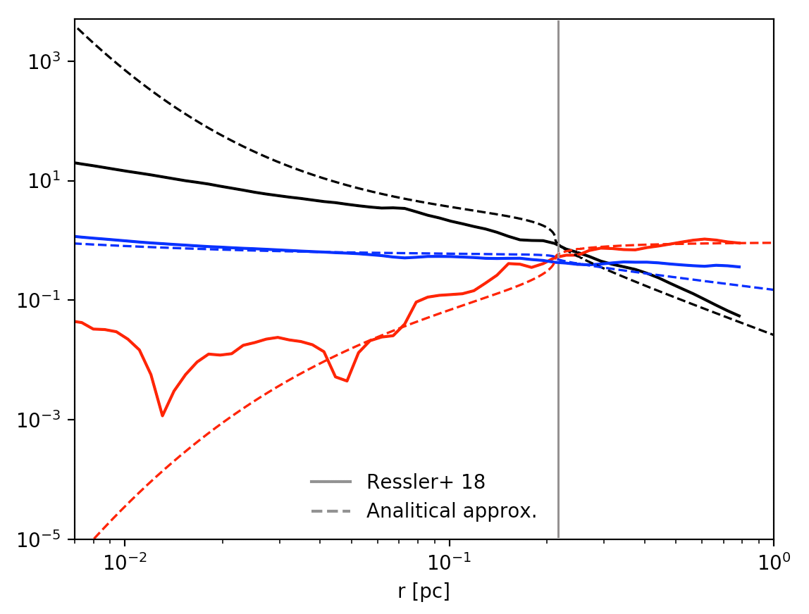
Figure 8: In this Figure we show the radial velocity in red (pc/kyr), the sound speed in blue (pc/kyr) and the density in black (M_⊙/pc³). The solid lines show the numerical results of Ressler, Quataert & Stone (2018) (their Figure 18). The dashed lines show our analytical model (derived from Section 2). The gray vertical line shows the cluster radius $R_{c}=0.22$ pc (which corresponds to $r_{c}=11.9$).

References

- Abuter et al. (2018) Gravity Collaboration; Auter, R., Amorim, A., Anugu, N., et al. 2018, A&A, 615, L15
- Baganoff et al. (2003) Baganoff, F. K., Maeda, Y., Morris, M., et al. 2003, ApJ, 591, 891
- Cantó et al. (2000) Cantó, J., Raga, A. C., Rodríguez, L. F. 2000, ApJ, 536, 896
- Cuadra et al. (2005) Cuadra, J., Nayakshin, S., Springel, V., et al. 2005, MNRAS, 360, L55
- Cuadra et al. (2006) Cuadra, J., Nayakshin, S., Springel, V., et al. 2006, MNRAS, 366, 358
- Cuadra, Nayakshin & Martins (2008) Cuadra, J., Nayakshin, S., & Martins, F. 2008, MNRAS, 383, 458
- Castellanos-Ramírez et al. (2015) Castellanos-Ramírez, A., Rodríguez-González, A.,Esquivel, A., et al. 2015, MNRAS, 450, 2799
- Chevalier & Clegg (1985) Chevalier, R. A., Clegg, A. W., 1985, Nature, 317, 44
- Dere et al. (1997) Dere, K. P., Landi, E., Mason, H. E., et al. 1997, A&AS, 125, 149
- Dere et al. (2019) Dere, K. P., Del Zanna, G., Young, P. R., et al. 2019, ApJS, 241, 22
- Esquivel et al. (2009) Esquivel, A., Raga A. C., Cantó J., Rodríguez-González A., 2009, A&A, 507, 855
- Esquivel & Raga (2013) Esquivel, A. & Raga A. C., 2013, ApJ, 779, 111
- Falle et al. (2012) Falle, S. A. E. G., Coker, R. F., Pittard, J.M., Dyson, J. E., Hartquist, T. W. 2002, MNRAS, 329, 670
- Genzel et al. (2003) Genzel, R., Schödel, R., Ott, T., et al. 2003, ApJ, 599, 812
- Ghez et al. (2005) Ghez A. M., Salim S., Hornstein S. D., et al. 2005, ApJ, 620, 744
- Hueyotl-Zahuantitla et al. (2010) Hueyotl-Zahuantitla, F., Palous, J., Wünsch, R. et al. 2010, ApJ, 766, 92
- Lora et al. (2009) Lora, V., Sánchez-Salcedo, F. J., Raga, A. C. & Esquivel, A., 2009, ApJL, 699, L113
- Lützgendorf et al. (2016) Lützgendorf, N., van der Helm, E., Pelupessy, F. I., et al. 2016, MNRAS, 456, 3645
- Martins et al. (2007) Martins F., Genzel R., Hillier D. J., Eisenhauer F., Paumard T.,Gillessen S., Ott T., Trippe S., 2007, A & A, 468, 233
- Palous̆ et al. (2013) Palous̆, J., Wünsch, R., Martínez-González, S., et al. 2013, ApJ, 772, 128
- Quataert (2004) Quataert, E. 2004, ApJ, 613, 344
- Raga et al. (2001) Raga, A. C., Velázquez, P. F., Cantó, J., Masciadri, E., Rodríguez, L. F. 2001, ApJ, 559, L33
- Ressler, Quataert & Stone (2018) Ressler, S. M., Quataert, E. & Stone, J. M. 2018, MNRAS, 478, 3544
- Ressler, Quataert & Stone (2020) Ressler, S. M., Quataert, E. & Stone, J. M. 2020, MNRAS, 492, 3272
- Rockefeller et al. (2004) Rockefeller, G., Fryer, C., Melia, F., Warren, M. S., 2004, ApJ, 604, 662
- Rodríguez-González et al. (2007) Rodríguez-González, A., Cantó, J., Esquivel, A., Raga, A. C., Velázquez, P. F. 2007, MNRAS, 380, 1198
- Rodríguez-González et al. (2008) Rodríguez-González, A., Esquivel, A.,Raga, A. C., Cantó, J. 2008, ApJ, 684, 1384
- Rodríguez-Ramírez et al. (2014) Rodríguez-Ramírez, J. C., Raga, A. C., Velázquez, P. F., Rodríguez-González, A., Toledo-Roy, J. C. 2014, MNRAS, 445, 1023