Nonlinear Tunable Vibrational Response in Hexagonal Boron Nitride

Abstract

Nonlinear light-matter interactions in structured materials are the source of exciting properties and enable vanguard applications in photonics. However, the magnitude of nonlinear effects is generally small, thus requiring high optical intensities for their manifestation at the nanoscale. Here, we reveal a large nonlinear response of monolayer hexagonal boron nitride (hBN) in the mid-infrared phonon-polariton region, triggered by the strongly anharmonic potential associated with atomic vibrations in this material. We present robust first-principles theory predicting a threshold light field $\sim 40\,$MV/m to produce order-unity effects in Kerr nonlinearities and harmonic generation, which are made possible by a combination of the long lifetimes exhibited by optical phonons and the strongly asymmetric landscape of the configuration energy in hBN. We further foresee polariton blockade at the few-quanta level in nanometer-sized structures. In addition, by mixing static and optical fields, the strong nonlinear response of monolayer hBN gives rise to substantial frequency shifts of optical phonon modes, exceeding their spectral width for in-plane DC fields that are attainable using lateral gating technology. We therefore predict a practical scheme for electrical tunability of the vibrational modes with potential interest in mid-infrared optoelectronics. The strong nonlinear response, low damping, and robustness of hBN polaritons set the stage for the development of applications in light modulation, sensing, and metrology, while triggering the search for intense vibrational nonlinear response in other ionic materials.

I Introduction

Major improvements in nanofabrication Nagpal et al. (2009); Duan et al. (2012); Davis et al. (2020) and colloid chemistry Burda et al. (2005); Cai et al. (2010) over the last two decades have enabled an extraordinary degree of control over the electromagnetic field associated with light at nanometer scales, well below the free-space light wavelength. These advances have facilitated the development of applications in fields such as optoelectronics Mak and Shan (2016), optical sensing Neumaier et al. (2015); Di Fabrizio et al. (2016); Yang et al. (2018a), photochemistry Clavero (2014), and light harvesting Atwater and Polman (2010) by exploiting the linear optical response of the involved materials. Nonlinear effects open up a wealth of possibilities in quantum optics Cox and García de Abajo (2018), harmonic generation Sivis et al. (2017), all-optical light modulation and switching Boyd (2008); Garmire (2013), and nonlinear microscopy Campagnola and Loew (2003); Wang et al. (2011); Dempsey et al. (2012); Staedler et al. (2012); Huang and Cheng (2013) and sensing Neely et al. (2009); Mesch et al. (2016); Di Fabrizio et al. (2016); Dhillon et al. (2017); Yu et al. (2016). Unfortunately, the nonlinear response of available materials is rather weak, so the manifestation of nonlinear phenomena generally demands their accumulation as light propagates across large structures (i.e., extending over many optical wavelengths Boyd (2008); Garmire (2013)), or alternatively, the use of intense optical fields. However, the light intensity that can be tolerated by nanostructures is limited due to heating damage, which can be effectively prevented by reducing the irradiation time, so understandably, progress in nonlinear optics has largely relied on the availability of ultrafast laser pulses with fluences $\lesssim 10\,$J/m².

Two-level atoms constitute the paramount example of a nonlinear system Boyd (2008) in which resonant photon absorption is prevented after it is formerly excited by a previous photon. However, individual atoms possess small transition strengths, as quantified by the f-sum rule Pines and Noziéres (1966), because only one electron is effectively involved in the excitation, thus resulting in poor coupling to light, and consequently, also a weak nonlinear response. Insulators and semiconductor materials can exhibit larger transition strength associated with a higher density of available valence electrons, and actually, there are notable examples among them offering relatively large nonlinear response combined with low optical absorption that enable applications such as optical parameter oscillators for frequency conversion Boyd (2008). The high density of conduction electrons in metals also translates into a larger transition strength, which, although accompanied by substantial optical absorption, still gives rise to relatively strong nonlinearities, particularly in noble metal nanostructures Uchida et al. (1994); Galletto et al. (1999); Russier-Antoine et al. (2007); Liu et al. (2006); Singh et al. (2009).

Localized optical resonances can produce amplification of the externally applied light intensity to enhance nonlinear effects Rodríguez Echarri et al. (2018). In particular, metal plasmons provide the means to amplify the near field intensity by several orders of magnitude, thus strongly increasing the nonlinear response Lippitz et al. (2005); Liu et al. (2006); Danckwerts and Novotny (2007); Schwartz and Oron (2009); Butet et al. (2010a, b); Stockman (2011); Harutyunyan et al. (2012); Kauranen and Zayats (2012). Unfortunately, metals suffer from large optical losses Khurgin (2015) that limit their lifetimes, so alternative less lossy materials have been explored, such as graphene, which can sustain electrically tunable Fei et al. (2012); Chen et al. (2012) and long-lived Ni et al. (2018) plasmons, while simultaneously featuring a strong nonlinear response because of the conic, anharmonic nature of its electronic band structure Mikhailov (2007); Mikhailov and Ziegler (2008). More precisely, graphene exhibits a large third-order susceptibility that manifests in relatively strong four-wave mixing Hendry et al. (2010); Gu et al. (2012); Constant et al. (2016), third-harmonic generation (THG)Kumar et al. (2013a); Hong et al. (2013); Soavi et al. (2018); Calafell et al. (2021), and the optical Kerr effect Zhang et al. (2012); Dremetsika et al. (2016). Although graphene plasmons have been only observed at low frequencies in the terahertz and mid-infrared domains, they can enhance the intrinsically large nonlinear response of their host material Cox and García de Abajo (2019); Calafell et al. (2021), with potential application in quantum optics Cox and García de Abajo (2018) and high-harmonic generation Cox et al. (2017).

The two-dimensionality of graphene is advantageous for nanophotonic devices because it facilitates exposure to the external optical field. Likewise, the vast family of two-dimensional (2D) transition metal dichalcogenides (TMDs) also host interesting nonlinear properties, as revealed by the observation of strong second-harmonic generation (SHG) in odd-layer films of MoS₂ Malard et al. (2013); Kumar et al. (2013b), MoSe₂ Chen et al. (2017), WS₂ Janisch et al. (2014), and WSe₂ Wang et al. (2015), as well as THG in MoS₂ Säynätjoki et al. (2017); Woodward et al. (2016) and spiral WS₂ Fan et al. (2017).

For sufficiently strong external fields, atomic vibrations in solids and molecules can be pushed beyond the harmonic regime, thus exhibiting nonlinear behavior. Surprisingly, harmonic generation associated with atomic vibrations has only been poorly explored, with just a few works focusing on this phenomenon at terahertz frequencies Dekorsy et al. (2003); Paarmann et al. (2016); Nicoletti and Cavalleri (2016); Winta et al. (2018), as well as a parallel effort on parametric amplification of optical phonons in SiC Cartella et al. (2018). The strength of vibrational nonlinear effects is a key question that determines the range of applications, but this line of research is still open, in search of robust materials with intense response. Mid-infrared nanophotonic devices would benefit from such strong nonlinearity, in particular in 2D platforms that enable easy access to the external field. In this context, hexagonal boron nitride (hBN) emerges as an appealing candidate that exhibits long-lived optical phonon polaritons, although their associated nonlinear response has not yet been assessed.

Here, we find that atomic vibrations in polar crystals can produce strong optical nonlinearities in the mid-infrared spectral region, on par with their electronic counterparts in strongly nonlinear media. We concentrate on monolayer hBN as a material of current interest due to its ability to host long-lived phonon polaritons at spectral bands emerging at around $\sim 100\,$meV and $\sim 170\,$meV. Through first-principles simulations, we find that the higher-energy band exhibits a substantial degree of asymmetry for atomic vibrations involving stretching of the B-N bond, giving rise to a strongly anharmonic behavior that translates into relatively intense harmonic generation, as well as sizeable Kerr nonlinearity. Phonon polaritons such as those in hBN therefore emerge as a promising platform for mid-infrared nonlinear optics, with applications that include harmonic generation, optical modulation, and quantum blockade at the few-quantum level in nanometer-sized structures, as well as active electrical modulation by applying DC lateral fields.

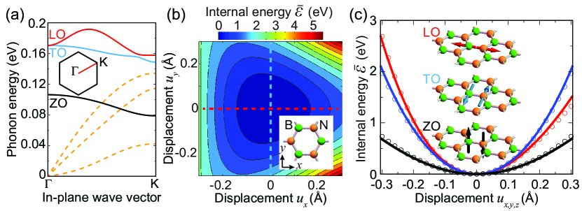
Figure 1: Anharmonicity in the atomic vibrations of monolayer hBN. (a) Linear dispersion relations of the three acoustic (dashed curves) and three optical (ZO, TO, and LO solid curves) phonon modes along the $\Gamma$-K direction (see first Brillouin zone in the inset) calculated from DFT (see Methods). (b) Total internal energy per unit cell as a function of in-plane relative B-N atomic displacement ${\bf u}$ at the $\Gamma$ point. We set the energy origin at the equilibrium configuration ${\bf u}=0$. (c) Color-coded cuts along the dashed lines in (b). For comparison, we also show the energy variation associated with out-of-plane motion (ZO mode, black curve and lowest inset). We plot DFT results (symbols) and polynomial fits (curves, see main text). The plot reveals strong non-parabolicity for motion along $x$ (LO mode).

II Results and Discussion

The dispersion diagram of monolayer hBN phonons contains three relatively high energy optical-phonon bands, one starting at $\sim 100\,$meV (ZO) and the other two above $\sim 170\,$meV (TO and LO), associated with atomic vibrations primarily involving motion perpendicular and parallel to the hexagonal atomic lattice plane, respectively. In this paper, we study vibrations at the $\Gamma$ point, where the two upper bands are degenerate (Figure 1a). Our treatment is exact when dealing with normally impinging light, but we argue that it also provides a good approximation to model strongly confined phonon-polaritons with in-plane wavelengths down to $\lambda_{\rm p}\sim 10$ nm, whose associated wave vectors $2\pi/\lambda_{\rm p}\sim 0.06\,{\AA}^{-1}$ are small compared with the wave vector at the K point $4\pi/3\sqrt{3}a\approx\,1.7{\AA}^{-1}$, where $a=1.446\,{\AA}$ is the B-N bond distance. We thus expect that the linear and nonlinear response functions derived from the present $\Gamma$-point analysis embody an accurate description of the optical properties of mid-infrared phonon-polaritons in monolayer hBN.

At the $\Gamma$ point, atoms in each crystal unit cell follow the same vibration pattern, which can be described in terms of the B-N relative displacement vector ${\bf u}$ according to the equation of motion (see Methods)

$$M\left[\ddot{{\bf u}}(t)+\tau^{-1}\dot{{\bf u}}(t)\right]=-\nabla_{{\bf u}}\left[\bar{\mathcal{E}}({\bf u})-\;\bar{{\bf p}}({\bf u})\cdot{\bf E}^{\rm ext}(t)\right],$$ (1)

where $M=M_{\rm B}M_{\rm N}/(M_{\rm B}+M_{\rm N})$ is the reduced mass, $\bar{\mathcal{E}}({\bf u})$ and $\bar{{\bf p}}({\bf u})$ are the displacement-dependent configuration energy and dipole per unit cell, respectively, ${\bf E}^{\rm ext}(t)$ is the electric field of the external light, and we introduce a phenomenological lifetime $\tau$. For concreteness, we take the B-N bond vector along $x$ with the B and N unit-cell atoms placed at $a\,\hat{\bf x}$ and $2a\,\hat{\bf x}$, respectively. For a given ${\bf u}$, the displacements of the two unit cell atoms are ${\bf u}_{\rm B}=-(M/M_{\rm B}){\bf u}$ and ${\bf u}_{\rm N}=(M/M_{\rm N}){\bf u}$ (i.e., positive $u_{x}$ corresponds to stretching), where $M_{\rm B}=10.811\,$Da and $M_{\rm N}=14.007\,$Da are the average masses corresponding to the natural isotopic abundances of these two elements. In what follows, we set $\tau=2\,$ps, which is consistent with the lifetimes observed in optical measurements Giles et al. (2018). In addition, we calculate $\bar{\mathcal{E}}({\bf u})$ and $\bar{{\bf p}}({\bf u})$ using density-functional theory (DFT), as explained in the Methods section. Because we focus on the $\Gamma$ point, atomic displacements preserve translational crystal symmetry, so DFT methods for infinite crystals can be straightforwardly applied. We concentrate on the upper optical phonon branches, associated with in-plane atomic motion (i.e., $u_{z}=0$). Retaining only up to quartic terms in $\bar{\mathcal{E}}$ and cubic terms in $\bar{\bf p}$ compatible with mirror symmetry relative to the $u_{y}=0$ line and three-fold crystal symmetry around $\hat{\bf z}$, our DFT calculations for $u\leq 0.03\,{\AA}$ lead to the fitted expressions

$$\bar{\mathcal{E}}({\bf u}) \approx e_{0}\,(u_{x}^{2}+u_{y}^{2})+e_{1}\,u_{x}(u_{x}^{2}-3u_{y}^{2})+e_{2}\,u^{4},$$ (2a)

$$\bar{{\bf p}}({\bf u}) \approx\bar{p}_{0}\,\hat{\bf x}+Q_{0}\,{\bf u}+Q_{1}\big{[}(u_{x}^{2}-u_{y}^{2})\,\hat{\bf x}-2\,u_{x}u_{y}\,\hat{\bf y}\big{]}+Q_{2}\,u^{2}\,{\bf u},$$ (2b)

with coefficients $e_{0}=0.2176$, $e_{1}=-0.1126$, $e_{2}=0.0489$, $\bar{p}_{0}=-0.6756$, $Q_{0}=-0.346$, $Q_{1}=-0.069$, and $Q_{2}=0.110$ expressed in atomic units. We note that ${\bf p}({\bf u})$ is accompanied by the external field in eq 1, so both of the expansions in eqs 2 account for corrections up third order in the external field. As a result of the crystal symmetries noted above, the energy landscape (Figure 1b) exhibits a more anharmonic profile for motion along $x$, as clearly observed when comparing cuts across $u_{x}=0$ and $u_{y}=0$ (Figure 1c). For completeness, we calculate (with coefficients in atomic units) $\bar{\mathcal{E}}\approx 0.0839\,u_{z}^{2}-0.0167\,u_{z}^{4}$ and $\bar{p}_{z}\approx-0.304\,u_{z}+0.194\,u_{z}^{3}$ for out-of-plane motion at $u_{x}=u_{y}=0$; these expressions reveal a more harmonic potential (i.e., smaller nonlinear effects) and a light-coupling dipole of similar strength in the ZO mode.

Equations 2 encapsulate all the information that is needed to study the vibrational dynamics driven by external illumination in the spectral region near the upper optical modes at the $\Gamma$ point according to eq 1. In particular, the corresponding unperturbed in-plane mode energy $\hbar\omega_{0}=\hbar\sqrt{2e_{0}/M}\approx 170\,$meV is in excellent agreement with previous theoretical Sohier et al. (2017) and experimental Rokuta et al. (1997); Cai et al. (2017) results. Incidentally, the permanent dipole $\bar{p}_{0}$ does not affect optical phonons at the $\Gamma$ point, although it contributes to the dynamics of acoustic modes.

In what follows, we study the response to a monochromatic external field ${\bf E}^{\rm ext}(t)=2{\bf E}_{0}\cos(\omega t)$ of frequency $\omega$ by solving eq 1 either perturbatively or in the time domain, thus yielding the time-dependent displacement vector ${\bf u}(t)$, and from here the unit-cell induced dipole $\bar{\bf p}({\bf u})-\bar{\bf p}(0)$, from which we extract the nonlinear response functions of monolayer hBN.

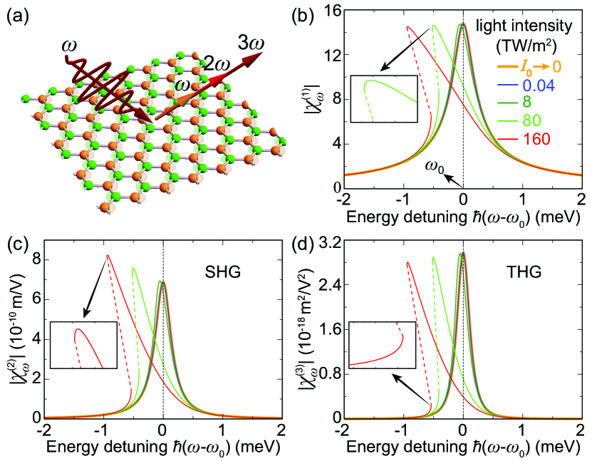
Figure 2: Nonlinear optical response of monolayer hBN in the upper optical-phonon region. (a) We consider normally impinging light with linear polarization along one of the B-N bond directions $x$. (b-d) Spectral dependence of the susceptibilities $\chi^{(s)}_{\omega}$ associated with the fundamental (b), SHG (c), and THG (d) frequencies ($s=1-3$, respectively) for a series of increasing incident light intensities (see legend in (b)). We show the low-intensity perturbative limit $\chi^{ss}_{\omega}$ for comparison (thick orange curves). The photon energy $\hbar\omega$ is referred to the linear mode resonance ($\hbar\omega_{0}\approx 170\,$meV). We assume a phonon lifetime of $\tau=2\,$ps (i.e., $\hbar\tau^{-1}\approx 0.33\,$meV).

Nonperturbative Nonlinear Response in Monolayer hBN

Based on the energy landscapes shown in Figure 1b,c, we expect a strong nonlinear response associated with atomic vibrations for in-plane displacement vectors oriented along $x$ (the unit-cell B-N bond direction). Because this is a symmetry axis, such vibrations are rigorously constrained to $u_{y}=u_{z}=0$ if the external field is also oriented along $x$, so inserting eqs 2 into eq 1 and plugging external monochromatic light of frequency $\omega$, the equation of motion reduces to

$$\ddot{u}_{x}+\tau^{-1}\dot{u}_{x}+\omega_{0}^{2}u_{x}+(3e_{1}/M)\,u_{x}^{2}+(4e_{2}/M)\,u_{x}^{3}$$

$$=(2/M)(Q_{0}+2Q_{1}u_{x}+3Q_{2}u_{x}^{2})\,E_{0}\cos(\omega t),$$ (3)

which is a generalization of the Duffing equation Tajaddodianfar et al. (2017). In Figure 2, we present results obtained by numerically integrating this equation as a function of $\omega$ for different levels of light intensity $I_{0}=2E_{0}^{2}/Z_{0}$, where $Z_{0}=\sqrt{\mu_{0}/\epsilon_{0}}\approx 376.73\,\Omega$ is the vacuum impedance. From the solution for the time-dependent displacement $u_{x}(t)$, we express the induced dipole (eq 2b) as $p_{x}(t)=Q_{0}u_{x}(t)+Q_{1}u_{x}^{2}(t)+Q_{2}u_{x}^{3}(t)$. In practice, we solve the above differential equation starting from some initial boundary conditions (see below) and integrating up to a large time $t=N\tau_{\omega}\gg\tau$ (expressed as a multiple of the optical period $\tau_{\omega}=2\pi/\omega$), so that the transient response produced after plugging the external light is attenuated to a negligible level. We then compute the susceptibility associated with a harmonic $s$ as

$$\chi^{(s)}_{\omega}=\frac{1}{\epsilon_{0}(E_{0})^{s}\mathcal{V}\tau_{\omega}}\int_{N\tau_{\omega}}^{(N+1)\tau_{\omega}}dt\;p_{x}(t)\;{\rm e}^{{\rm i}s\omega t},$$ (4)

where $\epsilon_{0}$ is the vacuum permittivity and we divide by a volume $\mathcal{V}=\mathcal{A}h$ given by the product of the unit cell area $\mathcal{A}=(3\sqrt{3}/2)\,a^{2}=5.43\,{\AA}^{2}$ and the layer thickness $h=3.3\,{\AA}$, with the latter approximated to the interatomic plane distance in bulk hBN.

At low intensities, the susceptibilities exhibit a Lorentzian profile of decreasing width as the harmonic order $s$ increases. Our numerical results converge well to the perturbative analytical limit (see Methods) for $I_{0}\rightarrow 0$ (thick orange curves in Figure 2b-d). When the intensity increases, the spectral peak is red shifted, and eventually, we reach a region of bistability. We explore this behavior by using the converged solution for each $\omega$ as the initial condition to calculate the response for a slightly different $\omega$; this leads to two branches, corresponding to increasing or decreasing frequency starting from -2 meV or 2 meV detuning, respectively. Such behavior is observed for all harmonics investigated in Figure 2. In the bistability region, a third unstable branch exists Boyd (2008), which we illustrate by dashed lines, introduced here as a guide to the eye. Nonpertubative effects are perceptible for light intensities $I_{0}\gtrsim 10\,$TW/m² (i.e., $E_{0}\gtrsim 40\,$MV/m).

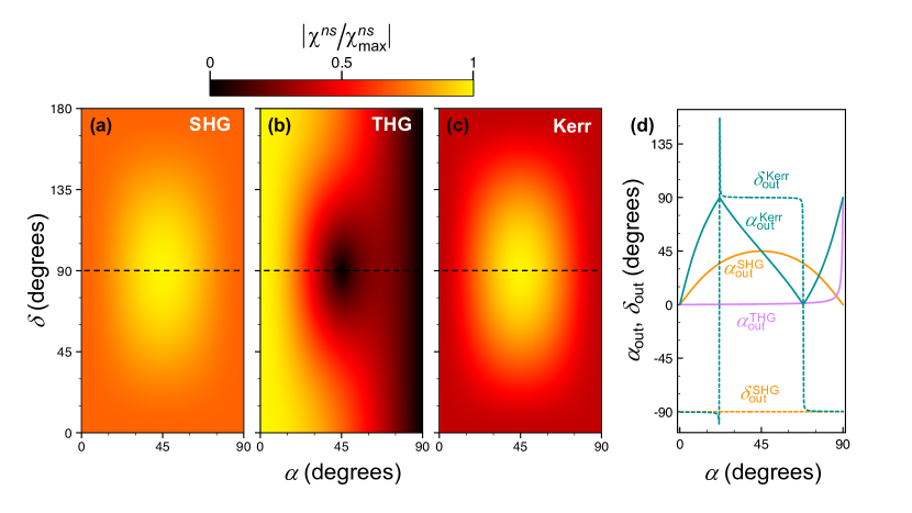
Figure 3: Polarization dependence of the nonlinear response. (a-c) Perturbative results for the dependence of the nonlinear susceptibility associated with SHG, THG, and the Kerr effect on the polarization of the external light under normal incidence on monolayer hBN. The polarization angles define the field amplitude as $\cos\alpha\,\hat{\bf x}+\sin\alpha\,{\rm e}^{{\rm i}\delta}\hat{\bf y}$. Maxima in the color scale correspond to $\chi^{22}_{\rm max}=9.7\times 10^{-10}\,$m/V, $\chi^{33}_{\rm max}=3.0\times 10^{-18}\,$m²/V², and $\chi^{31}_{\rm max}=8.3\times 10^{-15}\,$m²/V² for the SHG (a), THG (b), and Kerr (c) susceptibilities, assuming a polariton lifetime $\tau=2\,$ps. (d) Polarization angles of the output nonlinear components as a function of $\alpha$ for $\delta=90^{\circ}$ (i.e., along the dashed lines in (a-c)).

Polarization Dependence

The in-plane anisotropy of hBN translates into a strong dependence of the nonlinear response on light polarization, which we analyse in Figure 3. Specifically, we represent the perturbative susceptibilities associated with SHG, THG, and the Kerr effect (see Methods) for normally impinging light of frequency $\omega=\omega_{0}$ tuned to the in-plane $\Gamma$ phonon frequency as a function of polarization angles $(\alpha,\delta)$, defined in such a way that the incident field amplitude vector is proportional to $\cos\alpha\,\hat{\bf x}+\sin\alpha\,{\rm e}^{{\rm i}\delta}\hat{\bf y}$. The second-harmonic response (Figure 3a) is independent of the direction of the field amplitude for linear polarization ($\delta=0$), while an absolute maximum is observed for circularly polarized light (CPL, $\alpha=45^{\circ}$, $\delta=90^{\circ}$) with a relative enhancement of 41%. Interestingly, the polarization of the SHG signal under CPL irradiation is reversed (output polarization angles $\alpha_{\rm out}=45^{\circ}$, $\delta_{\rm out}=-90^{\circ}$; see Figure 3d). We find that THG (Figure 3b) is maximum for polarization along $x$ ($\delta=0$), where it is completely depleted for CPL, in agreement with the intuitive conclusions extracted from the anharmonicity observed in Figure 1c for oscillations parallel or perpendicular with respect to the B-N bond direction. We also analyze the third-order Kerr susceptibility (Figure 3c), which is maximal for CPL, in which case the polarization angles of the nonlinear Kerr response are the same as the incident ones (Figure 3d). Incidentally, right on resonance ($\omega=\omega_{0}$), we find that $\chi^{31}_{\omega_{0}}$ is $90^{\circ}$ out of phase relative to both $\chi^{11}_{\omega_{0}}$ and $\chi^{51}_{\omega_{0}}$ (see Methods), so the relative correction to the polarization intensity coming from the Kerr effect scales with the incident intensity as $I_{0}^{2}$, with contributions at that order arising from both ${\rm Re}\{\chi^{11*}_{\omega_{0}}\chi^{51}_{\omega_{0}}\}$ (i.e., through mixing with the linear amplitude) and $|\chi^{31}_{\omega_{0}}|^{2}$. This translates into a dependence of $|\chi^{(1)}|^{2}$ on $I_{0}$ as shown in Figure 4a (see also discussion in Methods), where the lowest-order correction (dashed curve for $s=1$, obtained by including $\chi^{31}_{\omega_{0}}$) leads to the wrong sign in the variation of the first-harmonic intensity, whereas the addition of $\chi^{51}$ (dotted curve) produces an initial depletion, in agreement with the nonperturbative result (solid curve), although this approximation eventually breaks down for larger incident intensity.

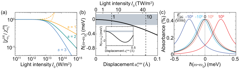
Figure 4: Nonlinear saturation of the optical response. (a) On-resonance susceptibilities $\chi^{(s)}_{\omega_{0}}$ associated with the fundamental ($s=1$), SHG ($s=2$), and THG ($s=3$) response as a function light intensity $I_{0}$ under the conditions of Figure 2, normalized to the low-$I_{0}$ limit $\chi^{ss}_{\omega_{0}}$. Analytical perturbative results are shown as broken curves, including the contribution of $\chi_{\omega_{0}}^{31}$ (dashed curve) and $\chi_{\omega_{0}}^{51}$ (dotted curve). (b) Amplitude dependence of the in-plane vibration frequency for motion along $x$. The lower horizontal axis corresponds to the maximum displacement, while the upper axis indicates the light intensity needed to reach it according to Figure 2b. The two dashed vertical lines indicate the $\sqrt{2}$ times the rms displacement in a $\sim 1\,$nm² island (18 unit cells) for a phonon population of 1 and 10 phonons, as indicated by labels. The shaded region indicates a FWHM corresponding to a lifetime $\tau=2\,$ps. (c) Spectral change in the linear absorbance spectrum of monolayer hBN produced by a uniform in-plane DC field along $x$ for different values of the field amplitudes.

Saturation and Quantum Blockade

The onset of saturation at $\sim 10\,$TW/m² is illustrated in Figure 4a, where we plot the susceptibilities associated with polarization emerging at the fundamental, SHG, and THG frequencies for on-resonance illumination at $\omega=\omega_{0}$. Saturation occurs faster as the harmonic order increases because this involves higher powers of the fundamental field amplitude. From a physical viewpoint, this plot essentially describes the combination of anharmonic oscillations and the effective coupling strength to external light. We find the first of these factors to be of interest per se because it affects the departure from harmonic behavior at the few-quanta level. In fact, this is the basis for the quantum blockade phenomenon, which we mentioned above for two-level systems: for a sufficiently anharmonic response, the energy of a two-quanta state differs from twice the energy of one quantum. Quantum blockade has been observed in cavity quantum electrodynamics experiments, whereby a two-level atom is coupled to an optical cavity Birnbaum et al. (2005), so that the system inherits a strong anharmoniticy from the former, as well as a large coupling to light from the latter. Incidentally, this type of effect has also been theoretically studied with graphene-plasmon cavities Manjavacas et al. (2012), a configuration in which Rabi vacuum splitting can be discernible Koppens et al. (2011), with a view to realizing quantum-optics devices in a solid-state environment by benefiting from the strong nonlinearity of this material. However, the fabrication of few-nanometer-sized graphene structures capable of sustaining high-quality plasmons remains an experimental challenge.

Atomic vibrations in monolayer hBN provide an excellent alternative to realize quantum blockade in compact structures, which can profit from the structural stability of this material, as well as from the long lifetime and optical strength of its phonon polaritons. We explore this possibility by estimating the oscillation frequency associated with a given maximum displacement (Figure 4b) (see Methods). Larger oscillation amplitudes initially lead to frequency redshifts as a result of the reduction in the interatomic potential relative to a perfect parabola, quantified through the $e_{1}<0$ term in eq 2a. We also indicate in this figure an estimate for the root mean square (rms) amplitude associated with the the in-plane optical phonon mode in a $\sim 1\,$nm² hBN island (18 unit cells) for an occupation of either 1 or 10 phonons (see Methods; the rms amplitude is proportional to $\sqrt{n/A}$, where $n$ is the phonon occupation number and $A$ is the area of the island). Incidentally, we multiply the rms displacement by $\sqrt{2}$ to compare with the maximum displacement used in the horizontal axis of Figure 4b. The latter produces a frequency shift that exceeds the FWHM of the resonance assuming a lifetime $\tau=2\,$ps, therefore indicating the onset of quantum blockade.

Electrical Tunability

A lateral DC field acting on the hBN monolayer along $x$ produces a change in the B-N bond distance to minimize energy. We argue that the strength of the in-plane DC field that can be applied through lateral gating can reach $\sim 10^{9}\,$V/m, which is one order of magnitude larger than the maximum optical field considered in Figure 2. Still, a resonant optical field of amplitude $2E_{0}\cos(\omega_{0}t)$ induces a maximum atomic displacement $\approx(2Q_{0}\tau/M\omega_{0})E_{0}$ assisted by the amplifying mechanism of spring motion, while the displacement due to a DC field of the same magnitude is a factor of $\omega_{0}\tau\sim 500$ smaller. Nevertheless, we show next that the effect is strong enough to shift the phonon resonance by more than its spectral width, therefore enabling a practical route towards electrical light modulation that could find application in optoelectronics. We start our analysis from eq 3 by substituting the applied field by $E_{\rm DC}+2E_{0}\cos(\omega_{0}t)$. The DC component $E_{\rm DC}$ can be readily absorbed in a new set of parameters $\omega_{0}$, $e_{1}$, $Q_{0}$, and $Q_{1}$, from which only the variation of $\omega_{0}$ produces a sizeable effect. Obviously, no constant force term can remain in eq 3, a condition from which we find an equilibrium displacement $u_{x}^{0}\approx Q_{0}E_{\rm DC}/M\omega_{0}^{2}$. Because of the lack of parabolicity of the confining potential (see Figure 2c), we expect a shift in the resonance frequency of in-plane phonon at the $\Gamma$ point; after some algebra, we find $\Delta\omega_{0}\approx(3Q_{0}e_{1}/M\omega_{0}^{2}-2Q_{1})E_{\rm DC}/M\omega_{0}$, which is linear in the DC field and reaches $\sim 0.26\,$meV for $E_{\rm DC}\sim 10^{9}\,$V/m. We also find that $E_{\rm DC}^{2}$ corrections amount to less than 1%, whereas the linear and nonlinear optical responses of the material just experience a rigid frequency shift by $\Delta\omega_{0}$, with their magnitudes remaining nearly unaffected. This is illustrated by examining the absorbance of monolayer hBN ($\approx(4\pi\epsilon_{0}h\omega/c){\rm Im}\{\chi^{(1)}_{\omega}\}$), which reveals a peak shift by nearly twice the spectral width when the DC field is varied in the $\pm 10^{9}\,$V/m range (Figure 4c). Therefore, we anticipate that lateral gating can be used as an efficient mechanism for light modulation in the mid-infrared regime using hBN vibrational modes.

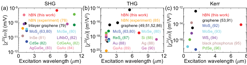
Figure 5: The nonlinear optical response of hBN in context. We compare the SHG, THG, and Kerr effect susceptibilities measured in different materials Kim et al. (2019); Shan et al. (2018); Autere et al. (2018); Woodward et al. (2016); Hao et al. (2019); Nikogosyan (2005); Harasaki and Kato (1997); Shoji et al. (1997); Popkova et al. (2021); Calafell et al. (2021); Kumar et al. (2013a); Soavi et al. (2018); Jiang et al. (2018); Cui et al. (2017); Bloembergen et al. (1969); Burns and Bloembergen (1971); Watkins et al. (1980); Zhang et al. (2012); Demetriou et al. (2016); Liu et al. (2015); Wang et al. (2014); Dong et al. (2016); Yang et al. (2018b); Jia et al. (2020) (see color-matching reference numbers in the legends) with our calculations for monolayer hBN at the in-plane $\Gamma$ phonon frequency.

III Concluding Remarks

In conclusion, we reveal monolayer hBN as an excellent nonlinear material at frequencies determined by its optical phonons. We base our results on first-principles predictive theory for the potential energy surface and induced dipole density in the material as a function of atomic positions. The optical response associated with atomic vibrations in monolayer hBN contains a substantial anharmonic component that gives rise to relatively intense second- and third-harmonic generation, as well as Kerr nonlinearity, as we show in comparison to existing experimental results for other 2D materials (Figure 5). We stress the fact that, in contrast to the nonlinear response arising from the electronic degrees of freedom, atomic vibrations offer a more robust platform with a lower level of optical losses. In particular, hBN can be compared with graphene, which operates in the same spectral range, but suffers from intrinsic losses that limit the external light intensities that can be applied without producing material damage. Atomic vibrations in hBN are indeed immune to strong optical absorption, such as that taking place in metallic systems, which leads to an elevation of the electronic temperature and an associated change in the optical response (i.e., an incoherent form of nonlinearity) that can mask and reduce the strength of coherent effects. Although graphene shows a larger nonlinear response associated with electronic degrees of freedom (Figure 5), we find hBN to be second best, and we argue that the vibrational origin of its optical response should permit elevating the applied light intensity with less heating of the material. We have focused on vibrations around the in-plane optical mode frequency in hBN, but we anticipate that future studies will explore other materials, covering a wide range of mid-infrared frequencies, and possibly hosting strongly nonlinear vibrational resonances.

Edges in finite hBN islands and defects in actual samples can modify the phonon characteristics, for example by producing localization at atomic scales Hage et al. (2020), which could affect the nonlinear response. Another interesting avenue consists in introducing strong in-plane DC fields to actively modify the nonlinear response, which we have predicted to enable phonon shifts exceeding their spectral width. In this respect, the insulator character of hBN should enable the presence of large lateral DC fields greatly exceeding those that are attainable through optical illumination. We have left aside thermal effects, which could also modify the nonlinear response, in particular in view of the fact that the in-plane mode population is $\sim 1$ at the melting temperature of hBN ($>2900$ K). The strong anharmonic response of hBN could be enhanced through resonant nanostructures Rodríguez Echarri et al. (2018), a possibility that deserves further exploration to assess the prospects for mid-infrared nonlinear nanophotonics, which could benefit from the strong interest that this material is currently attracting in the scientific community.

The isotopic purity of the material influences the phonon lifetime, and thus requires further investigation in connection to nonlinear effects. We have made some emphasis on the separation between the intrinsic anharmonic motion (i.e., the deviation in the potential energy surface from a parabolic profile) and the optical strength of the optical phonons (i.e., the dipole moment associated with atomic displacements). While the overall nonlinear response is the combined result of both of these aspects, we argue that the former needs to be examined separately, as it controls the possibility of having quantum blockade, whereby subsequent excitation is prevented by the nonlinear effects produced in response to previous excitations. In monolayer hBN, we find that nonlinear response at the few-quanta level is feasible by using structures of 1 nm lateral size, thus holding the potential for realizing quantum gates based on mid-infrared atomic vibrations in a robust solid-state material platform.

Appendix A Nonlinear Vibrational Optical Response

We examine the linear and nonlinear optical response associated with the atomic vibrations of monolayer hBN. The atomic scale under consideration is small compared with the light wavelength, so we work in the electrostatic limit and introduce the external light through an optical scalar potential $\phi^{\rm ext}({\bf r},t)$ acting on the B and N atoms (labeled by an index $l$), which oscillate around their equilibrium positions with time-dependent displacements ${\bf u}_{l}(t)$. For each configuration, defined by the set of the atomic displacements $\{{\bf u}\}$, we use DFT to calculate both the internal energy $\mathcal{E}(\{{\bf u}\})$ and the charge density distribution $\rho(\{{\bf u}\},{\bf r})$ (see below). Adopting the Born-Oppenheimer approximation to separate electronic and vibrational motions, and describing the latter classically, we write the Lagrangian of the system as $\mathcal{L}=(1/2)\sum_{l}M_{l}|\dot{{\bf u}}_{l}(t)|^{2}-\mathcal{E}(\{{\bf u}\})-\int d^{3}{\bf r}\;\rho(\{{\bf u}\},{\bf r})\;\phi^{\rm ext}({\bf r},t)$, where $M_{l}$ denotes the mass of atom $l$, whereas the integral term stands for the potential energy due to the interaction with the external potential. From the Lagrange equation $\partial_{t}\nabla_{\dot{{\bf u}}_{l}}\mathcal{L}=\nabla_{{\bf u}_{l}}\mathcal{L}$, we find

$$M_{l}\left[\ddot{{\bf u}}_{l}(t)+\tau^{-1}\dot{{\bf u}}_{l}(t)\right]=-\nabla_{{\bf u}_{l}}\left[\mathcal{E}(\{{\bf u}\})+\int d^{3}{\bf r}\;\rho(\{{\bf u}\},{\bf r})\;\phi^{\rm ext}({\bf r},t)\right],$$ (A5)

where we have introduced a phenomenological lifetime $\tau$ ($=2\,$ps in our calculations).

In the linear regime, we can approximate $\nabla_{{\bf u}_{l}}\mathcal{E}(\{{\bf u}\})\approx\sum_{l^{\prime}}\mathcal{D}_{ll^{\prime}}\cdot{\bf u}_{l^{\prime}}$ around the equilibrium configuration $\{{\bf u}=0\}$, where $\mathcal{D}_{ll^{\prime}}$ is the so-called dynamical matrix. The eigenvalues of this matrix define the phonon dispersion relations, as presented in Figure 1a for monolayer hBN based on our DFT calculations for $\mathcal{D}_{ll^{\prime}}$ (see below).

The wave vectors associated with far-field light or even tip-based illumination ($\sim 1/R_{\rm tip}<0.1\,$nm^-1 for a typical tip radius $R_{\rm tip}>10$ nm) are at least two orders of magnitude smaller than the reciprocal lattice vectors ($\geq 4\pi/3a\approx 29\,$nm^-1, where $a=1.446$ Å is the B-N bond distance), so for applications in photonics, we are generally interested in atomic vibrations close to the $\Gamma$ point (see Figure 1a). We thus study vibrations at this point as a good approximation to understand the nonlinear polaritonic dynamics in hBN. Under these conditions, the two atoms in each unit cell (B and N) move in the same way across the crystal, and therefore, we only need to consider a central unit cell with the atom label $l$ taking the values B or N. Clearly, the total potential (the quantity in square brackets in the right-hand side of eq A5) only depends on the relative coordinate ${\bf u}={\bf u}_{\rm N}-{\bf u}_{\rm B}$, whereas the center of mass moves at constant velocity. We thus have ${\bf u}_{\rm B}=-(M/M_{\rm B}){\bf u}\approx-0.564\,{\bf u}$ and ${\bf u}_{\rm N}=(M/M_{\rm N}){\bf u}\approx 0.436\,{\bf u}$, where $M=M_{\rm B}M_{\rm N}/(M_{\rm B}+M_{\rm N})\approx 6.102\,$Da is the reduced mass (assuming naturally abundant isotope distributions), while the equation of motion becomes

$$M\left[\ddot{{\bf u}}(t)+\tau^{-1}\dot{{\bf u}}(t)\right]=-\nabla_{{\bf u}}\left[\bar{\mathcal{E}}({\bf u})+\int_{\rm UC}d^{3}{\bf r}\;\rho({\bf u},{\bf r})\;\phi^{\rm ext}({\bf r},t)\right].$$ (A6)

Here, $\rho({\bf u},{\bf r})$ has the periodicity of the crystal, so the integral only extends over one unit cell (UC). Also, $\bar{\mathcal{E}}({\bf u})$ is the internal energy per unit cell, which we obtain from DFT (see below). Finally, based on the smallness of the wave vectors accessed through external illumination, we can approximate $\phi^{\rm ext}({\bf r},t)=-{\bf E}^{\rm ext}(t)\cdot{\bf r}$ in terms of an external electric field ${\bf E}^{\rm ext}(t)$, which allows us to rewrite eq A6 as in eq 1, where $\bar{{\bf p}}({\bf u})=\int_{\rm UC}d^{3}{\bf r}\;\rho({\bf u},{\bf r})\;{\bf r}$ is the unit cell dipole. In this work, we simulate the nonlinear response of monolayer hBN in the in-plane phonon spectral region by solving eq 1 together with the DFT-based parametrization given in eqs 2 for $\bar{\mathcal{E}}({\bf u})$ and $\bar{{\bf p}}({\bf u})$.

Appendix A DFT Calculations

We use the Vienna ab initio simulation package (VASP) Kresse and Furthmüller (1996a); Kresse and Hafner (1993); Kresse and Furthmüller (1996b) to carry out first-principles DFT calculations using the projector-augmented-wave (PAW) method Blöchl (1994) together with the generalized gradient approximation of Perdew-Burke-Ernzerhof (GGA-PBE) for the exchange-correlation functional Perdew et al. (1996). A vacuum spacing of 10 Å between adjacent images is introduced to prevent artificial interactions. The plane-wave energy cut-off is set to 500 eV. We use the conjugate gradient method to optimize the structure with an energy convergence criterion of $10^{-8}\,$eV between two ionic steps. A $\Gamma$-centered wave-vector sampling grid of size $18\times 18\times 1$ is used for the structural relaxation. Atomic positions and lattice vectors are relaxed until the total force in the unit cell is reduced to a value below $10^{-7}\,$eV/Å. The calculated B-N bond distance differs by just $+0.3\%$ from the measured value in bulk hBN. To obtain the charge density $\rho({\bf u},{\bf r})$, we calculate the electron densities corresponding to each atomic displacement using a sufficiently dense grid in the unit cell. The contribution from the nuclei and the K-shell electrons is incorporated by assimilating them to point charges ($3e$ for B and $5e$ for N), which add a term $\bar{\bf p}^{\rm nucl}({\bf u})=13ea\,\hat{\bf x}+eM(5/M_{\rm N}-3/M_{\rm B})\,{\bf u}$ to the unit cell dipole $\bar{\bf p}({\bf u})=\bar{\bf p}^{\rm el}({\bf u})+\bar{\bf p}^{\rm nucl}({\bf u})$, where $\bar{\bf p}^{\rm el}({\bf u})$ originates in the 8 outer electrons per unit cell. The result from this analysis for in-plane atomic displacements is well described by the polynomial expressions in eqs 2, which are compatible with the crystal symmetries of the hBN monolayer. The linear phonon frequencies and the dynamical matrix are calculated using the small displacement method.

Table 1: Peak nonlinear susceptibility in the perturbative regime. We focus on polarization along the $x$ direction (parallel to B-N bonds) and consider different incoming light frequencies $\omega_{\rm in}$, harmonics $s\omega_{\rm in}$, and perturbation orders $n$. The $\Delta\omega_{\rm in}$ column gives the FWHM of the $\big{|}\chi^{ns}_{\omega_{\rm in}}\big{|}^{2}$ as a function of incident frequency. The rightmost column shows the corresponding values of the susceptibilities in SI units for $\tau=2\,$ps.

$\omega_{\rm in}$	$(n,s)$	$s\omega_{\rm in}$	$\chi^{ns}_{\omega_{\rm in}}$	$\Delta\omega_{\rm in}$	$|\chi^{ns}_{\omega_{\rm in}}|$ (mn-1/Vn-1)
$\omega_{0}$	(1,1)	$\omega_{0}$	$\propto\tau$	$1/\tau$	$14.8$
$\omega_{0}$	(2,2)	$2\omega_{0}$	$\propto\tau^{2}$	$\approx 0.64/\tau$	$6.88\times 10^{-10}$
$\omega_{0}$	(3,3)	$3\omega_{0}$	$\propto\tau^{3}$	$\approx 1/2\tau$	$2.97\times 10^{-18}$
$\omega_{0}$	(3,1)	$\omega_{0}$	$\propto\tau^{4}$	$\approx 0.44/\tau$	$3.22\times 10^{-15}$
$\omega_{0}/2$	(2,2)	$\omega_{0}$	$\propto\tau$	$1/2\tau$	$4.37\times 10^{-11}$
$\omega_{0}/2$	(3,3)	$3\omega_{0}/2$	$\propto\tau$	$1/2\tau$	$9.73\times 10^{-23}$
$\omega_{0}/3$	(3,3)	$\omega_{0}$	$\propto\tau$	$1/3\tau$	$1.30\times 10^{-22}$

Appendix A Perturbation Limit

We find a perturbative solution to eq 1 by expanding the displacement vector as ${\bf u}=\sum_{ns}{\bf u}^{ns}{\rm e}^{-{\rm i}s\omega t}$, where $n$ is the scattering order and $s$ is the harmonic, subject to the condition $|s|\leq n$. For a monochromatic field ${\bf E}^{\rm ext}(t)=2{\bf E}_{0}\cos(\omega t)$, this leads to the recurrence relation

$$M\,\big{[}\omega_{0}^{2}-s\omega(s\omega+{\rm i}\tau^{-1})\big{]} \,u_{i}^{ns}=-e_{1}\sum_{jk}\sum_{n^{\prime}s^{\prime}}a_{ijk}u_{j}^{n^{\prime}s^{\prime}}u_{k}^{n-n^{\prime},s-s^{\prime}}$$

$$-e_{2}\sum_{jkl}\sum_{n^{\prime}s^{\prime}n^{\prime\prime}s^{\prime\prime}}b_{ijkl}u_{j}^{n^{\prime}s^{\prime}}u_{k}^{n^{\prime\prime}s^{\prime\prime}}u_{l}^{n-n^{\prime}-n^{\prime\prime},s-s^{\prime}-s^{\prime\prime}}$$

$$+Q_{0}\delta_{n,1}\big{(}\delta_{s,1}E_{0,i}+\delta_{s,-1}E_{0,i}^{*}\big{)}$$

$$+Q_{1}\sum_{j}c_{ijk}\big{(}u_{j}^{n-1,s-1}E_{0,k}+u_{j}^{n-1,s+1}E_{0,k}^{*}\big{)}$$

$$+Q_{2}\sum_{jkl}\sum_{n^{\prime}s^{\prime}}d_{ijkl}u_{j}^{n^{\prime}s^{\prime}}\big{(}u_{k}^{n-n^{\prime}-1,s-s^{\prime}-1}E_{0,l}+u_{k}^{n-n^{\prime}-1,s-s^{\prime}+1}E_{0,l}^{*}\big{)},$$

where $i,j,k,l\in\{x,y,z\}$ denote Cartesian components and the only nonzero coefficients inside the sums (extracted from eqs 2) are $a_{xxx}=-a_{yxy}/2=-a_{xyy}=3$, $b_{xxxx}=b_{xxyy}=b_{yyxx}=b_{yyyy}=4$, $c_{xxx}=-c_{yyx}=-c_{xyy}=-c_{yxy}=2$, $d_{xxxx}=d_{yyyy}=3$, $d_{yxyx}=d_{xxyy}=2$, and $d_{xyyx}=d_{yxxy}=1$. Incidentally, this equation leads to the vanishing of $u_{i}^{ns}$ if $n+s$ is odd. Through iterative solution, we obtain the displacement components $u_{i}^{ns}$, which upon insertion into eq 2b, also produce analytical expressions for the induced dipole. In particular, for incident polarization along $x$, the displacement vectors are found to be confined along $x$ as well, and we obtain the perturbation series

$$\frac{p_{x}(t)}{\epsilon_{0}\mathcal{V}}=\sum_{s}\chi^{(s)}_{\omega}E_{0}^{s}{\rm e}^{-{\rm i}s\omega t}$$

for the polarization density, where we define the field-dependent harmonic susceptibilities $\chi^{(s)}_{\omega}=\sum_{n}\chi^{ns}_{\omega}|E_{0}|^{n-s}$, which should coincide with eq 4. For incidence frequency near $\omega_{0}$, the leading terms in the perturbation series are those involving the higher powers in the resonant factor $\big{[}\omega_{0}^{2}-\omega(\omega+{\rm i}\tau^{-1})\big{]}^{-1}$, namely,

$$\chi^{11}_{\omega} \approx\frac{Q_{0}^{2}}{\epsilon_{0}\mathcal{V}M}\frac{1}{\omega_{0}^{2}-\omega(\omega+{\rm i}\tau^{-1})},$$ (A7a)

$$\chi^{22}_{\omega} \approx\frac{Q_{0}^{3}}{\epsilon_{0}\mathcal{V}M^{2}}\bigg{(}\frac{e_{1}}{M\omega_{0}^{2}}+\frac{Q_{1}}{Q_{0}}\bigg{)}\frac{1}{\big{[}\omega_{0}^{2}-\omega(\omega+{\rm i}\tau^{-1})\big{]}^{2}},$$ (A7b)

$$\chi^{33}_{\omega} \approx\frac{{\rm i}Q_{0}^{4}}{4\epsilon_{0}\mathcal{V}M^{4}\omega_{0}^{2}}\bigg{(}2e_{2}+\frac{8e_{1}Q_{1}}{Q_{0}}+\frac{3e_{1}^{2}}{M\omega_{0}^{2}}+\frac{4MQ_{2}\omega_{0}^{2}}{Q_{0}}\bigg{)}\frac{1}{\big{[}\omega_{0}^{2}-\omega(\omega+{\rm i}\tau^{-1})\big{]}^{3}},$$ (A7c)

$$\chi^{31}_{\omega} \approx\frac{6Q_{0}^{4}}{\epsilon_{0}\mathcal{V}M^{4}}\bigg{(}\frac{5e_{1}^{2}}{M\omega_{0}^{2}}-2e_{2}\bigg{)}\frac{1}{\big{[}\omega_{0}^{2}-\omega(\omega+{\rm i}\tau^{-1})\big{]}^{2}\big{|}\omega_{0}^{2}-\omega(\omega+{\rm i}\tau^{-1})\big{|}^{2}}.$$ (A7d)

These expressions are in excellent agreement with the numerical solution of the equation of motion (eq 1) for low field intensity (see Figure 2). Their scaling with the lifetime $\tau$ is summarized in Table 1, along with explicit values at $\omega=\omega_{0}$.

Incidentally, for the on-resonance Kerr effect, we have $\chi^{(1)}_{\omega_{0}}=\chi^{11}_{\omega_{0}}+\chi^{31}_{\omega_{0}}|E_{0}|^{2}+\chi^{51}_{\omega_{0}}|E_{0}|^{4}+\dots$, contributed by odd-order susceptibilities

$$\chi^{11}_{\omega_{0}} =\frac{iQ_{0}^{2}\tau}{\epsilon_{0}\mathcal{V}M\omega_{0}},$$

$$\chi^{31}_{\omega_{0}} =-\frac{6Q_{0}^{4}\tau^{4}}{\epsilon_{0}\mathcal{V}M^{4}\omega_{0}^{4}}\left(5e_{1}^{2}/M\omega_{0}^{2}-2e_{2}\right),$$

$$\chi^{51}_{\omega_{0}} =-\frac{36iQ_{0}^{6}\tau^{7}}{\epsilon_{0}\mathcal{V}M^{7}\omega_{0}^{7}}\left(5e_{1}^{2}/M\omega_{0}^{2}-2e_{2}\right)^{2}.$$

The $n=3$ term is $90^{\circ}$ out of phase with respect to $n=1$, and thus, these two do not interfere in the resulting intensity $I^{(1)}\propto|\chi^{(1)}_{\omega_{0}}|^{2}$. Actually, for low $E_{0}$, the $n=3$ contribution produces an increase in $I^{(1)}$, which is however compensated by the $n=5$ term (see Figure 4a and discussion in the main text). Nevertheless, for sufficiently off-resonance $\omega$, the perturbative result embodied in eq A7d reproduces the decay of the curves in Fig. 2(b) away from the resonance (not shown).

Appendix A Phonon Quantization and Quantum Blockade

In the linear regime, the potential energy can be approximated by the quadratic expression $\mathcal{E}(\{{\bf u}\})=(1/2)\sum_{ll^{\prime}}{\bf u}_{l}\cdot\mathcal{D}_{ll^{\prime}}\cdot{\bf u}_{l^{\prime}}$, so in the absence of external illumination, the solution to the classical equation of motion (eq A5) admits an expansion ${\bf u}_{l}=M_{l}^{-1/2}\sum_{n}c_{n}{\bf e}_{nl}$ in terms of a complete ($\sum_{n}{\bf e}_{nl}\otimes{\bf e}_{nl^{\prime}}=\delta_{ll^{\prime}}\mathcal{I}_{3}$) and orthonormal ($\sum_{l}{\bf e}_{nl}\cdot{\bf e}_{n^{\prime}l}=\delta_{nn^{\prime}}$) basis set of eigenvectors ${\bf e}_{nl}$ of the real, symmetric dynamical matrix (i.e., $\sum_{l^{\prime}}(M_{l}M_{l^{\prime}})^{-1/2}\mathcal{D}_{ll^{\prime}}\cdot{\bf e}_{nl^{\prime}}=\omega_{n}^{2}{\bf e}_{nl}$, where $\omega_{n}$ are real oscillation eigenfrequencies). In a quantum description, we can write the Hamiltonian associated with atomic vibrations in general as $\hat{\mathcal{H}}=-\sum_{l}\hbar^{2}\nabla_{{\bf u}_{l}}^{2}/2M_{l}+\mathcal{E}(\{{\bf u}\})=(1/2)\sum_{n}\big{(}-\hbar^{2}\nabla^{2}_{c_{n}c_{n}}+\omega_{n}^{2}c_{n}^{2}\big{)}$, where the rightmost expression, obtained by replacing the displacement vectors by the expansion coefficients $c_{n}=\sum_{l}\sqrt{M_{l}}{\bf e}_{nl}\cdot{\bf u}_{l}$, consists of a sum over quantum harmonic oscillators. Following a standard second quantization procedure, we interpret $c_{n}$ and $-{\rm i}\hbar\partial_{c_{n}}$ as displacement and momentum operators, respectively, from which we define phonon creation and annihilation operators $\hat{b}_{n}^{\dagger}$ and $\hat{b}_{n}$ through $c_{n}=\sqrt{\hbar/(2\omega_{n})}(\hat{b}_{n}^{\dagger}+\hat{b}_{n})$ and $-{\rm i}\hbar\partial_{c_{n}}={\rm i}\sqrt{\hbar\omega_{n}/2}(\hat{b}_{n}^{\dagger}-\hat{b}_{n})$, in terms of which the Hamiltonian reduces to $\hat{\mathcal{H}}=\hbar\sum_{n}\omega_{n}(\hat{b}_{n}^{\dagger}\hat{b}_{n}+1/2)$. The rms displacement of atom $l$ associated with the presence of one phonon in mode $n$ is thus given by $\sqrt{\langle 0|\hat{b}_{n}|{\bf u}_{l}|^{2}\hat{b}_{n}^{\dagger}|0\rangle}=\sqrt{3\hbar/(2M_{l}\omega_{n})}\,|{\bf e}_{nl}|$, where we have used the noted expansion of ${\bf u}_{l}$ in terms of eigenmodes, and the expansion coefficients $c_{n}$ in terms of ladder operators. For a hBN flake consisting of a finite number $N$ of unit cells, approximating the eigenvectors to those of an infinite crystal, orthornormality implies $|{\bf e}_{nl}|\sim 1/\sqrt{N}$, and in particular, for oscillations at the $\Gamma$ point, the rms displacement associated with one quantum reduces to $\sqrt{\langle u^{2}\rangle}\approx\sqrt{3\hbar/(2NM\omega_{0})}$.

Appendix A Oscillation Frequency beyond the Linear Regime

Focusing on atomic motion along $x$, we find the self-sustained oscillation frequency by multiplying eq 3 by the velocity $\dot{u}_{x}$, neglecting losses ($\tau^{-1}=0$) and setting the external drive to zero ($E_{0}=0$). As a function of the maximum displacement $u_{x}^{\rm max}>0$ toward the positive $x$ direction, where the potential is lower (see Figure 1a), direct integration then yields the oscillation period $T=2\int_{u_{x}^{\rm min}}^{u_{x}^{\rm max}}du_{x}/\sqrt{f(u_{x}^{\rm max})-f(u_{x})}$, where $f(u_{x})=\omega_{0}^{2}u_{x}^{2}+(2e_{1}/M)\,u_{x}^{3}+(2e_{2}/M)\,u_{x}^{4}$ and $u_{x}^{\rm min}<0$ is the lower bound of the oscillation defined by $f(u_{x}^{\rm min})=f(u_{x}^{\rm max})$. We find $u_{x}^{\rm min}$ from the analytical solution of resulting polynomial of the fourth degree, and then numerical integrate the above expression to obtain the oscillation frequency $\omega=2\pi/T$, plotted in Figure 4b as function of $u_{x}^{\rm max}$.

References

- Nagpal et al. (2009) P. Nagpal, N. C. Lindquist, S.-H. Oh, and D. J. Norris, Science 325, 594 (2009).
- Duan et al. (2012) H. Duan, A. I. Fernández-Domínguez, M. Bosman, S. A. Maier, and J. K. W. Yang, Nano Lett. 12, 1683 (2012).
- Davis et al. (2020) T. J. Davis, D. Janoschka, P. Dreher, B. Frank, F.-J. Meyer zu Heringdorf, and H. Giessen, Science 368, eaba6415 (2020).
- Burda et al. (2005) C. Burda, X. Chen, R. Narayanan, and M. A. El-Sayed, Chem. Rev. 105, 1025 (2005).
- Cai et al. (2010) J. Cai, P. Ruffieux, R. Jaafar, M. Bieri, T. Braun, S. Blankenburg, M. Muoth, A. P. Seitsonen, M. Saleh, X. Feng, et al., Nature 466, 470 (2010).
- Mak and Shan (2016) K. F. Mak and J. Shan, Nat. Photon. 10, 216 (2016).
- Neumaier et al. (2015) P. F.-X. Neumaier, K. Schmalz, J. Borngräber, R. Wylde, and H.-W. Hübers, Analyst 140, 213 (2015).
- Di Fabrizio et al. (2016) E. Di Fabrizio, S. Schlücker, J. Wenger, R. Regmi, H. Rigneault, G. Calafiore, M. West, S. Cabrini, M. Fleischer, N. F. Van Hulst, et al., J. Opt. 18, 063003 (2016).
- Yang et al. (2018a) X. Yang, Z. Sun, T. Low, H. Hu, X. Guo, F. J. García de Abajo, P. Avouris, and Q. Dai, Adv. Mater. 30, 1704896 (2018a).
- Clavero (2014) C. Clavero, Nat. Photon. 8, 95 (2014).
- Atwater and Polman (2010) H. A. Atwater and A. Polman, Nat. Mater. 9, 205 (2010).
- Cox and García de Abajo (2018) J. D. Cox and F. J. García de Abajo, Phys. Rev. Lett. 121, 257403 (2018).
- Sivis et al. (2017) M. Sivis, M. Taucer, G. Vampa, K. Johnston, A. Staudte, A. Y. Naumov, D. M. Villeneuve, C. Ropers, and P. B. Corkum, Science 357, 303 (2017).
- Boyd (2008) R. W. Boyd, Nonlinear Optics (Academic Press, Amsterdam, 2008), 3rd ed.
- Garmire (2013) E. Garmire, Opt. Express 21, 30532 (2013).
- Campagnola and Loew (2003) P. J. Campagnola and L. M. Loew, Nat. Biotech. 21, 1356 (2003).
- Wang et al. (2011) Y. Wang, C.-Y. Lin, A. Nikolaenko, V. Raghunathan, and E. O. Potma, Adv. Opt. Photon. 3, 1 (2011).
- Dempsey et al. (2012) W. P. Dempsey, S. E. Fraser, and P. Pantazis, Bioessays 34, 351 (2012).
- Staedler et al. (2012) D. Staedler, T. Magouroux, R. Hadji, C. Joulaud, J. Extermann, S. Schwung, S. Passemard, C. Kasparian, G. Clarke, M. Gerrmann, et al., ACS Nano 6, 2542 (2012).
- Huang and Cheng (2013) L. Huang and J.-X. Cheng, Annu. Rev. Mater. Res. 43, 213 (2013).
- Neely et al. (2009) A. Neely, C. Perry, B. Varisli, A. K. Singh, T. Arbneshi, D. Senapati, J. R. Kalluri, and P. C. Ray, ACS Nano 3, 2834 (2009).
- Mesch et al. (2016) M. Mesch, B. Metzger, M. Hentschel, and H. Giessen, Nano Lett. 16, 3155 (2016).
- Dhillon et al. (2017) S. S. Dhillon, M. S. Vitiello, E. H. Linfield, A. G. Davies, M. C. Hoffmann, J. Booske, C. Paoloni, M. Gensch, P. Weightman, G. P. Williams, et al., J. Phys. D: Appl. Phys. 50, 043001 (2017).
- Yu et al. (2016) R. Yu, J. D. Cox, and F. J. García de Abajo, Phys. Rev. Lett. 117, 123904 (2016).
- Pines and Noziéres (1966) D. Pines and P. Noziéres, The Theory of Quantum Liquids (W. A. Benjamin, Inc., New York, 1966).
- Uchida et al. (1994) K. Uchida, S. Kaneko, S. Omi, C. Hata, H. Tanji, Y. Asahara, A. J. Ikushima, T. Tokizaki, and A. Nakamura, J. Opt. Soc. Am. B 11, 1236 (1994).
- Galletto et al. (1999) P. Galletto, P. F. Brevet, H. H. Girault, R. Antoine, and M. Broyer, Chem. Commun. pp. 581–582 (1999).
- Russier-Antoine et al. (2007) I. Russier-Antoine, E. Benichou, G. Bachelier, C. Jonin, and P. F. Brevet, J. Phys. Chem. C 111, 9044 (2007).
- Liu et al. (2006) T.-M. Liu, S.-P. Tai, C.-H. Yu, Y.-C. Wen, S.-W. Chu, L.-J. Chen, M. R. Prasad, K.-J. Lin, and C.-K. Sun, Appl. Phys. Lett. 89, 043122 (2006).
- Singh et al. (2009) A. K. Singh, D. Senapati, A. Neely, G. Kolawole, C. Hawker, and P. C. Ray, Chem. Phys. Lett. 481, 94 (2009).
- Rodríguez Echarri et al. (2018) A. Rodríguez Echarri, J. D. Cox, R. Yu, and F. J. García de Abajo, ACS Photonics 5, 1521 (2018).
- Lippitz et al. (2005) M. Lippitz, M. A. van Dijk, and M. Orrit, Nano Lett. 5, 799 (2005).
- Danckwerts and Novotny (2007) M. Danckwerts and L. Novotny, Phys. Rev. Lett. 98, 026104 (2007).
- Schwartz and Oron (2009) O. Schwartz and D. Oron, Nano Lett. 9, 4093 (2009).
- Butet et al. (2010a) J. Butet, J. Duboisset, G. Bachelier, I. Russier-Antoine, E. Benichou, C. Jonin, and P.-F. Brevet, Nano Lett. 10, 1717 (2010a).
- Butet et al. (2010b) J. Butet, G. Bachelier, I. Russier-Antoine, C. Jonin, E. Benichou, and P.-F. Brevet, Phys. Rev. Lett. 105, 077401 (2010b).
- Stockman (2011) M. I. Stockman, Opt. Express 19, 22029 (2011).
- Harutyunyan et al. (2012) H. Harutyunyan, G. Volpe, R. Quidant, and L. Novotny, Phys. Rev. Lett. 108, 217403 (2012).
- Kauranen and Zayats (2012) M. Kauranen and A. V. Zayats, Nat. Photon. 6, 737 (2012).
- Khurgin (2015) J. B. Khurgin, Nat. Nanotech. 10, 2 (2015).
- Fei et al. (2012) Z. Fei, A. S. Rodin, G. O. Andreev, W. Bao, A. S. McLeod, M. Wagner, L. M. Zhang, Z. Zhao, M. Thiemens, G. Dominguez, et al., Nature 487, 82 (2012).
- Chen et al. (2012) J. Chen, M. Badioli, P. Alonso-González, S. Thongrattanasiri, F. Huth, J. Osmond, M. Spasenović, A. Centeno, A. Pesquera, P. Godignon, et al., Nature 487, 77 (2012).
- Ni et al. (2018) G. X. Ni, A. S. McLeod, Z. Sun, L. Wang, L. Xiong, K. W. Post, S. S. Sunku, B.-Y. Jiang, J. Hone, C. R. Dean, et al., Nature 557, 530 (2018).
- Mikhailov (2007) S. A. Mikhailov, Europhys. Lett. 79, 27002 (2007).
- Mikhailov and Ziegler (2008) S. A. Mikhailov and K. Ziegler, J. Phys. Condens. Matter 20, 384204 (2008).
- Hendry et al. (2010) E. Hendry, P. J. Hale, J. Moger, A. K. Savchenko, and S. A. Mikhailov, Phys. Rev. Lett. 105, 097401 (2010).
- Gu et al. (2012) T. Gu, N. Petrone, J. F. McMillan, A. van der Zande, M. Yu, G. Q. Lo, D. L. Kwong, J. Hone, and C. W. Wong, Nat. Photon. 6, 554 (2012).
- Constant et al. (2016) T. J. Constant, S. M. Hornett, D. E. Chang, and E. Hendry, Nat. Phys. 12, 124 (2016).
- Kumar et al. (2013a) N. Kumar, J. Kumar, C. Gerstenkorn, R. Wang, H.-Y. Chiu, A. L. Smirl, and H. Zhao, Phys. Rev. B 87, 121406(R) (2013a).
- Hong et al. (2013) S.-Y. Hong, J. I. Dadap, N. Petrone, P.-C. Yeh, J. Hone, and R. M. Osgood, Jr., Phys. Rev. X 3, 021014 (2013).
- Soavi et al. (2018) G. Soavi, G. Wang, H. Rostami, D. G. Purdie, D. De Fazio, T. Ma, B. Luo, J. Wang, A. K. Ott, D. Yoon, et al., Nat. Nanotech. 13, 583 (2018).
- Calafell et al. (2021) I. A. Calafell, L. A. Rozema, D. A. Iranzo, A. Trenti, P. K. Jenke, J. D. Cox, A. Kumar, H. Bieliaiev, S. Nanot, C. Peng, et al., Nat. Nanotech. 16, 318 (2021).
- Zhang et al. (2012) H. Zhang, S. Virally, Q. Bao, L. K. Ping, S. Massar, N. Godbout, and P. Kockaert, Opt. Lett. 37, 1856 (2012).
- Dremetsika et al. (2016) E. Dremetsika, B. Dlubak, S.-P. Gorza, C. Ciret, M.-B. Martin, S. Hofmann, P. Seneor, D. Dolfi, S. Massar, P. Emplit, et al., Opt. Lett. 41, 3281 (2016).
- Cox and García de Abajo (2019) J. D. Cox and F. J. García de Abajo, Acc. Chem. Res. 52, 2536 (2019).
- Cox et al. (2017) J. D. Cox, A. Marini, and F. J. García de Abajo, Nat. Commun. 8, 14380 (2017).
- Malard et al. (2013) L. M. Malard, T. V. Alencar, A. P. M. Barboza, K. F. Mak, and A. M. de Paula, Phys. Rev. B 87, 201401 (2013).
- Kumar et al. (2013b) N. Kumar, Q. C. S. Najmaei, F. Ceballos, P. M. Ajayan, J. Lou, and H. Zhao, Phys. Rev. B 87, 161403 (2013b).
- Chen et al. (2017) H. Chen, V. Corboliou, A. S. Solntsev, D.-Y. Choi, M. A. Vincenti, D. de Ceglia, C. de Angelis, Y. Lu, and D. N. Neshev, Light: Sci. Appl. 6, e17060 (2017).
- Janisch et al. (2014) C. Janisch, Y. Wang, D. Ma, N. Mehta, A. L. Elías, N. Perea-López, M. Terrones, V. Crespi, and Z. Liu, Sci. Rep. 4, 5530 (2014).
- Wang et al. (2015) G. Wang, X. Marie, I. Gerber, T. Amand, D. Lagarde, L. Bouet, M. Vidal, A. Balocchi, and B. Urbaszek, Phys. Rev. Lett. 114, 097403 (2015).
- Säynätjoki et al. (2017) A. Säynätjoki, L. Karvonen, H. Rostami, A. Autere, S. Mehravar, A. Lombardo, R. A. Norwood, T. Hasan, N. Peyghambarian, H. Lipsanen, et al., Nat. Commun. 8, 893 (2017).
- Woodward et al. (2016) R. I. Woodward, R. T. Murray, C. F. Phelan, R. E. P. de Oliveira, T. H. Runcorn, E. J. R. Kelleher, S. Li, E. C. de Oliveira, G. J. M. Fechine, G. Eda, et al., 2D Mater. 4, 011006 (2016).
- Fan et al. (2017) X. Fan, Y. Jiang, X. Zhuang, H. Liu, T. Xu, W. Zheng, P. Fan, H. Li, X. Wu, X. Zhu, et al., ACS Nano 11, 4892 (2017).
- Dekorsy et al. (2003) T. Dekorsy, V. A. Yakovlev, W. Seidel, M. Helm, and F. Keilmann, Phys. Rev. Lett. 90, 055508 (2003).
- Paarmann et al. (2016) A. Paarmann, I. Razdolski, S. Gewinner, W. Schöllkopf, and M. Wolf, Phys. Rev. B 94, 134312 (2016).
- Nicoletti and Cavalleri (2016) D. Nicoletti and A. Cavalleri, Adv. Opt. Photonics 8, 401 (2016).
- Winta et al. (2018) C. J. Winta, S. Gewinner, W. Schöllkopf, M. Wolf, and A. Paarmann, Phys. Rev. B 97, 094108 (2018).
- Cartella et al. (2018) A. Cartella, T. F. Nova, M. Fechner, R. Merlin, and A. Cavalleri, Proc. Natl. Academ. Sci. 115, 12148 (2018).
- Giles et al. (2018) A. J. Giles, S. Dai, I. Vurgaftman, T. Hoffman, S. Liu, L. Lindsay, C. T. Ellis, N. Assefa, I. Chatzakis, T. L. Reinecke, et al., Nat. Mater. 17, 134 (2018).
- Sohier et al. (2017) T. Sohier, M. Gibertini, M. Calandra, F. Mauri, and N. Marzari, Nano Lett. 17, 3758 (2017).
- Rokuta et al. (1997) E. Rokuta, Y. Hasegawa, K. Suzuki, Y. Gamou, and C. Oshima, Phys. Rev. Lett. 79, 4609 (1997).
- Cai et al. (2017) Q. Cai, D. Scullion, A. Falin, K. Watanabe, T. Taniguchi, Y. Chen, E. J. G. Santos, and L. H. Li, Nanoscale 9, 3059 (2017).
- Tajaddodianfar et al. (2017) F. Tajaddodianfar, M. R. H. Yazdi, and H. N. Pishkenari, Microsyst. Technol. 23, 1913 (2017).
- Birnbaum et al. (2005) K. M. Birnbaum, A. Boca, R. Miller, A. D. Boozer, T. E. Northup, and H. J. Kimble, Nature 436, 87 (2005).
- Manjavacas et al. (2012) A. Manjavacas, P. Nordlander, and F. J. García de Abajo, ACS Nano 6, 1724 (2012).
- Koppens et al. (2011) F. H. L. Koppens, D. E. Chang, and F. J. García de Abajo, Nano Lett. 11, 3370 (2011).
- Kim et al. (2019) S. Kim, J. E. Fröch, A. Gardner, C. Li, I. Aharonovich, and A. S. Solntsev, Opt. Lett. 44, 5792 (2019).
- Shan et al. (2018) Y. Shan, Y. Li, D. Huang, Q. Tong, W. Yao, W.-T. Liu, and S. Wu, Sci. Adv. 4, eaat0074 (2018).
- Autere et al. (2018) A. Autere, H. Jussila, A. Marini, J. R. M. Saavedra, Y. Dai, A. Säynätjoki, L. Karvonen, H. Yang, B. Amirsolaimani, R. A. Norwood, et al., Phys. Rev. B 98, 115426 (2018).
- Hao et al. (2019) Q. Hao, H. Yi, H. Su, B. Wei, Z. Wang, Z. Lao, Y. Chai, Z. Wang, C. Jin, J. Dai, et al., Nano Lett. 19, 2634 (2019).
- Nikogosyan (2005) D. N. Nikogosyan, Nonlinear Optical Crystals: A Complete Survey (Springer-Verlag, New York, 2005).
- Harasaki and Kato (1997) A. Harasaki and K. Kato, Jpn. J. Appl. Phys. 36, 700 (1997).
- Shoji et al. (1997) I. Shoji, T. Kondo, A. Kitamoto, M. Shirane, and R. Ito, J. Opt. Soc. Am. B 14, 2268 (1997).
- Popkova et al. (2021) A. A. Popkova, I. M. Antropov, J. E. Fröch, S. Kim, I. Aharonovich, V. O. Bessonov, A. S. Solntsev, and A. A. Fedyanin, ACS Photonics p. https://doi.org/10.1021/acsphotonics.0c01759 (2021).
- Jiang et al. (2018) T. Jiang, D. Huang, J. Cheng, X. Fan, Z. Zhang, Y. Shan, Y. Yi, Y. Dai, L. Shi, K. Liu, et al., Nat. Photon. 559, 343 (2018).
- Cui et al. (2017) Q. Cui, R. A. Muniz, J. Sipe, and H. Zhao, Phys. Rev. B 95, 165406 (2017).
- Bloembergen et al. (1969) N. Bloembergen, W. Burns, and M. Matsuoka, Opt. Commun. 1, 195 (1969).
- Burns and Bloembergen (1971) W. Burns and N. Bloembergen, Phys. Rev. B 4, 3437 (1971).
- Watkins et al. (1980) D. Watkins, C. Phipps, and S. Thomas, Opt. Lett. 5, 248 (1980).
- Demetriou et al. (2016) G. Demetriou, H. T. Bookey, F. Biancalana, E. Abraham, Y. Wang, W. Ji, and A. K. Kar, Opt. Express 24, 13033 (2016).
- Liu et al. (2015) L. Liu, K. Xu, X. Wan, J. Xu, C. Y. Wong, and H. K. Tsang, Photonics Res. 3, 206 (2015).
- Wang et al. (2014) K. Wang, Y. Feng, C. Chang, J. Zhan, C. Wang, Q. Zhao, J. N. Coleman, L. Zhang, W. J. Blau, and J. Wang, Nanoscale 6, 10530 (2014).
- Dong et al. (2016) N. Dong, Y. Li, S. Zhang, N. McEvoy, X. Zhang, Y. Cui, L. Zhang, G. S. Duesberg, and J. Wang, Opt. Lett. 41, 3936 (2016).
- Yang et al. (2018b) T. Yang, I. Abdelwahab, H. Lin, Y. Bao, S. J. Rong Tan, S. Fraser, K. P. Loh, and B. Jia, ACS Photonics 5, 4969 (2018b).
- Jia et al. (2020) L. Jia, J. Wu, T. Yang, B. Jia, and D. J. Moss, ACS Appl. Nano Mater. 3, 6876 (2020).
- Hage et al. (2020) F. S. Hage, G. Radtke, D. M. Kepaptsoglou, M. Lazzeri, and Q. M. Ramasse, Science 367, 1124 (2020).
- Kresse and Furthmüller (1996a) G. Kresse and J. Furthmüller, Phys. Rev. B 54, 11169 (1996a).
- Kresse and Hafner (1993) G. Kresse and J. Hafner, Phys. Rev. B 47, 558 (1993).
- Kresse and Furthmüller (1996b) G. Kresse and J. Furthmüller, Comput. Mater. Sci. 6, 15 (1996b).
- Blöchl (1994) P. E. Blöchl, Phys. Rev. B 50, 17953 (1994).
- Perdew et al. (1996) J. P. Perdew, K. Burke, and M. Ernzerhof, Phys. Rev. Lett. 77, 3865 (1996).