A Data-Efficient Approach to Behind-the-Meter Solar Generation Disaggregation

Abstract.

With the emergence of cost effective battery storage and the decline in the solar photovoltaic (PV) levelized cost of energy (LCOE), the number of behind-the-meter solar PV systems is expected to increase steadily. The ability to estimate solar generation from these latent systems is crucial for a range of applications, including distribution system planning and operation, demand response, and non-intrusive load monitoring (NILM). This paper investigates the problem of disaggregating solar generation from smart meter data when historical disaggregated data from the target home is unavailable, and deployment characteristics of the PV system are unknown. The proposed approach entails inferring the physical characteristics from smart meter data and disaggregating solar generation using an iterative algorithm. This algorithm takes advantage of solar generation data (aka proxy measurements) from a few sites that are located in the same area as the target home, and solar generation data synthesized using a physical PV model. We evaluate our methods with 4 different proxy settings on around 160 homes in the United States and Australia, and show that the solar disaggregation accuracy is improved by 32.31% and 15.66% over two state-of-the-art methods using only one real proxy along with three synthetic proxies. Furthermore, we demonstrate that using the disaggregated home load rather than the net load data could improve the overall accuracy of three popular NILM methods by at least 22%.

1. Introduction

Solar photovoltaic (PV) generation is the fastest growing renewable energy source today (International Energy Agency, 2020). Almost half of this growth is projected to be behind-the-meter (BTM) installations, which are typically PV systems on the roof of homes and buildings (de Hoog et al., 2020). High penetration of PV systems introduces new challenges for planning and operation of power distribution networks, requiring the system operators and electric utilities to develop low-cost techniques for forecasting and monitoring the solar power injected into their feeders. These techniques should rely on the data that is commonly available to the utilities, in particular weather information and net meter data (i.e., home load minus solar generation) from advanced metering infrastructure with time resolutions in the range of one minute to one hour (Chen et al., 2020).

Several methods are proposed in the literature to estimate the solar power generated by BTM PV systems. They can be divided into three major categories:

1. Methods that rely on satellite and aerial imagery (de Hoog et al., 2020) to identify PV systems and estimate their physical characteristics, e.g., size, tilt, and orientation. These approaches provide a rough estimate of the peak production capacity, but cannot accurately estimate solar generation at a given time.

2. Methods that rely on a few separately metered solar sites in a geographical area to estimate the total solar generation in that area (Shaker et al., 2016a, b). These methods require the knowledge of the total installed capacity of PV systems in the area, which is not available in many cases.

3. Methods that apply signal separation techniques to disaggregate solar generation from feeder-level measurement or smart meter data (Chen et al., 2017; Cheung et al., 2018). The main advantage of the solar disaggregation methods that only require smart meter data is that they are widely applicable as they do not require additional information.

Solar disaggregation is closely related to non-intrusive load monitoring (NILM) (Hart, 1992), the problem of separating a household’s total energy consumption, measured by a single meter, into individual appliance consumption data. Despite the apparent analogy between the two problems, NILM methods cannot be directly applied to separate solar generation from home load. This is partly because most NILM methods assume that the operation of each appliance can be divided into a finite number of operating states (e.g., ON, OFF, standby), and that the power consumption in each state is known and constant. Solar generation however changes continuously depending on several factors, such as solar radiation and temperature, and can have abrupt changes due to the effect of passing clouds. This diminishes the efficacy of NILM methods (Dinesh et al., 2017). Furthermore, solar generation is subtracted from the home load, whereas appliance loads are summed to construct the home load. This ‘negative’ load confuses many NILM methods. Thus, it is necessary to develop reliable solar disaggregation methods to decompose the net load data into solar generation and home load. The NILM methods can then be applied to the latter component to identify the energy consumption of different appliances.

In this paper we propose a solar disaggregation method to accurately estimate the output of a BTM PV system in an offline fashion. Our method has two key advantages over prior work on solar disaggregation. First, it requires active power measurements with low temporal resolution, which is already collected by ordinary smart meters, and proxy measurements from only one or a few PV systems located in the same geographical area. This is motivated by the strong correlation between the outputs of PV systems located in the same city even if their deployment characteristics are not identical. Utilities often have access to direct solar measurements from several sites in a city, which can provide proxy measurements for solar disaggregation. Second, our method has a low computational overhead compared to the optimization-based methods proposed in the literature, making it suitable for large scale implementation. Our contribution is threefold:

• We propose a solar disaggregation method that merely relies on net load data and just a small number of separately metered solar PV systems in the same geographical area. We show that real proxy measurements can be replaced with synthetic ones to achieve comparable performance as long as there is one real proxy.

• We compare our method against other state-of-the-art methods using two publicly available datasets. We find that the proposed method outperforms the baselines in terms of disaggregation accuracy.

• We examine how the improved accuracy of solar disaggregation affects the accuracy of three baseline NILM methods, namely Factorial Hidden Markov Model (FHMM) (Kim et al., 2011), Sequence-to-Point (Seq2Point) (Zhang et al., 2018), and Denoising Autoencoder (DAE) (Kelly et al., 2015).

To our knowledge, there is no prior work that quantifies the improvement in the accuracy of NILM techniques when they run on the disaggregated home load rather than the net load measured by a smart meter. Our results confirm that performing solar disaggregation prior to NILM offers clear benefits.

2. Related Work

2.1. Solar Disaggregation

Solar disaggregation methods can be categorized based on the type of models they use for estimating solar power. In the first category, a physics-based model is used to estimate solar generation. The model parameters are typically inferred from the available data. Reference (Chen et al., 2017) uses the PV system’s location and net load data to build a model for maximum clear sky solar generation. It then estimates the true solar generation using a general weather model to account for the percentage reduction in the clear sky solar irradiance due to clouds, humidity, precipitation, etc. The method requires net load data from two days with clear sky and low energy consumption that have a large temperature difference. A solar disaggregation toolkit based on (Chen et al., 2017) is developed in (Bashir et al., 2019), which is used as a baseline in our work.

Reference (Kabir et al., 2019) proposes an unsupervised solar disaggregation framework that does not require net load data or the location of the PV system (i.e., its latitude and longitude). Instead, the authors estimate the home load by using a physical PV model together with Hidden Markov Model Regression. They start with an initial guess of the physical PV model parameters and iteratively estimate the home load and solar generation from the net load data. This method can achieve satisfactory performance after many iterations, which makes it too slow for real-world applications. In addition, accurate weather and irradiance data from the vicinity of the the target home are necessary for accurate disaggregation. We use this method as a baseline. The authors extend this work in (Kabir et al., 2021) to jointly disaggregate the net load data of a group of customers into aggregated solar generation and aggregated home load.

In the second category of solar disaggregation methods, a data-driven black-box model is used for the solar generation. Some of the methods rely on the aggregate data at the feeder, distribution or substation transformer level (Tabone et al., 2018; Kara et al., 2018; Bu et al., 2020a). The common shortcoming of these methods is that they are not accurate enough for disaggregating a single home’s net load. A promising method that disaggregates solar generation in the frequency domain is proposed in (Sossan et al., 2018). This method is also more suitable for feeder-level disaggregation because high resolution data are not commonly available at the customer level.

There are many methods that rely on customer-level net meter data. Reference (Cheung et al., 2018) uses a mixture model of representative customers without PV systems to model demands of customers with PV systems. The authors extend this work in (Chueng et al., 2020) by considering BTM battery storage. In recent work (Bu et al., 2020b), a disaggregation method is proposed based on the observation that there is a strong correlation between monthly nocturnal and diurnal home loads. Leveraging this, the authors estimate the customer’s monthly solar generation and subsequently their hourly solar generation. A shortcoming of this method is that each customer has some unique characteristics that cannot be captured using the home loads of other customers. This could lower the accuracy of this disaggregation method. On the plus side, it does not require any historical home load or solar generation data from the target home. It relies on low resolution smart meter data and a number of solar proxies. In this respect, it is similar to our disaggregation method. However, the performance of this method is only tested when several solar proxies are available. In contrast, our method can work with only one solar proxy, thanks to additional synthetic proxies that we take advantage of. Despite the novelty of this approach, we cannot use it as a baseline because the proposed method requires 3 years of data, which is not included in the two datasets we used. Besides, the publicly available version of the dataset used in that paper only contains the aggregated household demand at secondary distribution transformers.

2.2. NILM

Since the early days of smart meter rollouts, NILM has been extensively studied in the literature. At a high level, NILM methods aim to disaggregate the net load measured at a single point of measurement. A wide range of sampling rates are explored in the literature, from less than 1Hz to thousands of Hz. Despite the recent efforts in high frequency range (Völker et al., 2020; Singh et al., 2020), and the intuition that sampling the load profiles at high rates provides more useful features for NILM, collecting this data requires special hardware. The smart meter devices that are being installed widely in distribution grids can only provide low resolution data. A recent study concludes that the data sampled at 1/30 Hz would be sufficient to achieve a high accuracy in NILM (Huchtkoetter et al., 2020). It is also mentioned that such a low sampling rate allows the NILM algorithms to benefit from additional information pertaining to the past power consumption of some long-running appliances. A NILM method is proposed in (Shi et al., 2019) that is suitable for low-resolution data. The performance of this method is evaluated for a range of resolutions, from 5 minutes to 1 hour.

Since combining the temporal information with active power measurements can facilitate disaggregation (Gu-yuan Lin et al., 2010), most recent work utilizes Hidden Markov Model (HMM) and Deep Neural Networks (DNN). Reference (Kim et al., 2011) studies four variants of HMM for energy disaggregation using low frequency data. Another low frequency power disaggregation method is proposed in (Mauch et al., 2016) that is based on HMM and DNN. Reference (Kelly et al., 2015) studies different deep learning architectures for NILM. These methods can only generalize to unseen homes if the training set has enough variety, which is rare in NILM training sets. Reference (Zhang et al., 2018) proposes a sequence-to-point learning via a Convolutional Neural Network (CNN) that outperforms the sequence-to-sequence method introduced in (Kelly et al., 2015). Reference (Kukunuri et al., 2020) studies different DNN compression schemas and suggests a multi-task learning-based architecture to further compress the models.

The majority of NILM methods assume that the net load is simply the total power consumed by home appliances. There is just a few NILM papers that consider BTM solar generation. Reference (Wang et al., 2020) proposes a method to disaggregate three types of loads, namely traditional loads, distributed generation (e.g., PVs), and flexible loads (e.g., electric vehicles), at the substation level. However, the focus of our work is on customer-level solar disaggregation. The closest line of work to ours is by Dinesh et. al (Dinesh et al., 2017), which proposes a NILM method for customers with BTM solar generation. The authors construct a unique set of signatures for appliances and solar generation, and classify their operating modes using a spectral clustering based method. Finally, they identify their state and operating mode through a subspace component power level matching algorithm. The main drawback of this approach is that it relies on the synthesized net load measured at 1 second intervals. This is much faster than the sampling rate of smart meters that are currently installed in many jurisdictions (which is typically in the order of minutes).

3. Problem Definition

Customer-level solar disaggregation concerns decomposing the customer’s net load, presumably measured by a smart meter, into home load and solar generation. Since historical (disaggregated) data regarding solar generation and home load may not be available from a customer with a BTM PV system, the problem should be solved in an unsupervised or semi-supervised fashion.

3.1. Notation

As a general rule, matrices and vectors are denoted respectively by bold face uppercase and lowercase letters. We use a subscript to refer to a specific row of a matrix or an element of a vector.

Let $\textbf{y}\in\mathbb{R}^{T}$ be a vector that collects the measured net load of one customer over $T$ intervals. Hence, $\textbf{y}_{t}$ denotes the net load measurement of this customer at time $t\in\{1,2,...T\}$. Similarly, let $\hat{\bm{\ell}},\hat{\textbf{s}}\in\mathbb{R}^{T}$ denote respectively their estimated home load and behind-the-meter solar generation in the same period. These quantities must satisfy the following equality constraint: $\textbf{y}=\hat{\bm{\ell}}-\hat{\textbf{s}}$.

Let $\textbf{X}^{L}\in\mathbb{R}^{T\times K_{l}}$ be the set of $K_{l}$ features that determine the customer’s home load, and $\textbf{X}^{S}\in\mathbb{R}^{T\times K_{s}}$ be the set of $K_{s}$ proxy measurements that can be used to approximate the customer’s solar generation via a mixture model. We can train a non-linear model $g$ to map the features to the home load, and a linear solar mixture model to estimate the customer’s solar generation. The model $g$ can be a neural network, a support vector machine, a random forest, or any other nonlinear model used for regression. We can write:

(1) $$\hat{\bm{\ell}} =g(\textbf{X}^{L};\bm{\theta}),$$

(2) $$\hat{\textbf{s}} =\textbf{X}^{S}\textbf{w},$$

where $\bm{\theta}$ is a vector that represents parameters of the load model, and $\textbf{w}\in\mathbb{R}^{K_{s}}$ is the weight vector of the mixture model. Hence, $\textbf{w}_{k}$ is a scalar that represents the weight assigned to the $k^{\text{th}}$ proxy. The motivation for using a linear mixture model for estimating solar generation is explained in Section 4.1.

3.2. Assumptions

We postulate that no information is available about the customers except their approximate location (i.e., the city or district they are located in) and their smart meter data. Hence, we do not know the exact longitude and latitude information of each customer. This is a reasonable assumption because (a) some customers are reluctant to provide their home address, and (b) there might be data privacy requirements that prevent the utility from sharing their address with a third party that performs solar disaggregation or NILM. In addition to the smart meter data, solar irradiance, wind speed, and ambient temperature at the city scale can be downloaded via an API. We assume that deployment characteristics of BTM PV systems are not known a priori. These include the panel size, orientation, tilt, temperature coefficient, etc.

We assume that there is at least one separately metered solar installation in the same city or district as our target home. This site provides proxy measurements that are used to estimate solar generation of the target home. The deployment characteristics of this site could differ from the characteristics of the PV system installed at the target home. We argue that this is not a strong assumption as utilities usually have access to direct solar measurements from several sites in a city. Moreover, the cost of installing and maintaining one or a few PV systems can be easily justified by the potential benefits of observing customer-level PV generation.

4. methodology

We now introduce the models we use for estimating solar generation and home load. We present our solar disaggregation algorithm, which has two main parts: a weight initialization technique and an iterative algorithm for updating the model parameters.

4.1. Models

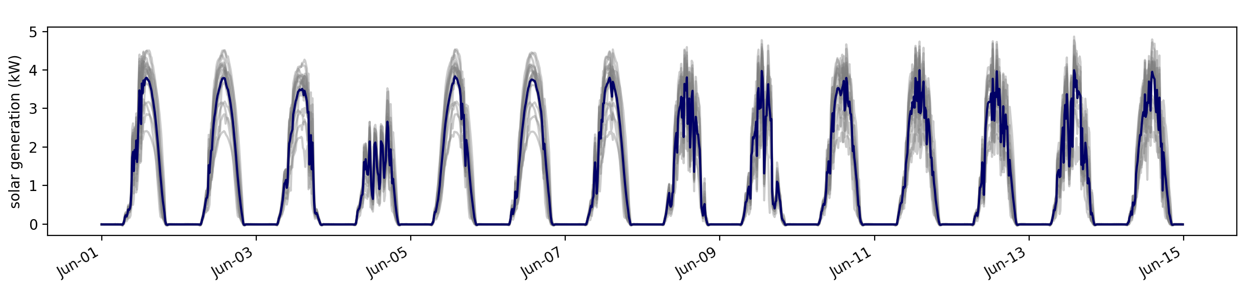
Figure 1. The solar generation of 19 homes in the Pecan Street dataset over 2 weeks. The thicker line shows the average solar generation across all the homes.

Solar mixture model: We aim to approximate that solar power generated by the BTM PV system installed at the target home using a mixture of proxy measurements from PV systems located in the same city or district. The intuition behind this approximation is that PV systems in the same geographical area have more or less the same solar generation pattern regardless of their deployment characteristics. This can be verified by inspection of Figure 1 which displays the solar power generated by 19 homes with BTM PV systems in Austin, Texas. The PV systems that have the same orientation but different sizes and tilts have almost identical solar generation patterns, though with different scales.

There are two specific challenges that must be addressed to get a good approximation. First, we do not have control over the deployment characteristics of the PV systems that provide proxy measurements. If they had exactly the same orientation angle as the PV system installed at the target home, estimating the target home’s solar generation would reduce to learning a single scaling factor. One way to address this challenge is to adopt a solar mixture model to approximate the target home’s solar generation as a weighted sum of a number of proxy measurements, as shown in Equation (2). This increases the chance of getting proxy measurements from PV systems with similar deployment characteristics to the target home. A higher weight will be eventually assigned to these PV systems in the mixture model. The second challenge is that proxy measurements from a large number of neighbouring PV systems might not be available in practice. To address this challenge, we combine proxy measurements from real PV systems with measurements synthesized by a physical PV model that takes into account solar irradiance data of an arbitrary location in the same city. We discuss in Section 6 that it is essential to use proxy measurements from at least one real PV system as some fluctuations in solar generation cannot be accurately explained by the physical PV model when coarse-grained solar irradiance data is fed to this model. We also demonstrate the importance of incorporating synthetic proxies that have different orientation angles in Figure 5. These synthetic proxies help us estimate the peak time of solar generation more accurately.

The physical PV model that we use to obtain data for synthetic proxies is based on PVWatts (Dobos, 2014). We develop this model using the PV Performance Modeling Collaborative (Stein, 2012). The output power of the PV model with the specified rating $P_{dc0}$ can be computed given the transmitted plane of array (POA) irradiance $I_{tr}$ and cell temperature $T_{cell}$:

(3) $$P_{dc}=\frac{I_{tr}}{E_{ref}}P_{dc0}(1+\gamma(T_{cell}-T_{ref}))$$

Here $\gamma$ represents the temperature coefficient, $E_{ref}$ represents the reference irradiance, and $T_{ref}$ represents the reference cell temperature. We set them respectively to -0.47%/${}^{\circ}C$, 1000W/$m^{2}$, and 25${}^{\circ}C$ to create synthetic proxies. $I_{tr}$ is determined by solar irradiance data (direct normal irradiance, diffuse horizontal irradiance, global horizontal irradiance), PV system characteristics (e.g., tilt, orientation) and its location. $T_{cell}$ is a function of wind speed, ambient air temperature, and solar irradiance data. We use different preset technical parameters for different synthetic proxies.

Home load model: To estimate the home load, we adopt a random forest regression, which is a supervised learning algorithm that uses an ensemble learning method for regression. We use the scikit-learn (Pedregosa et al., 2011) library to train this model. Four explanatory variables are used as features, $\textbf{X}^{L}$, for all customers. These variables include ambient temperature c, exponentially weighted moving average of temperature over the last 24 hours $\textbf{c}_{wmv}$, hour of the day h, and a binary variable d that indicates if it is a weekday or weekend. Thus, we have $\textbf{X}^{L}=[\textbf{c},\textbf{c}_{wmv},\textbf{h},\textbf{d}]$.

4.2. Solar Disaggregation

Weight initialization: The first step for implementing our method is to initialize the weight vector w of the solar mixture model using the net load data of the target home and the solar generation data collected from the proxies. A good initialization can enhance the performance of the disaggregation method and reduce its convergence time. Our weight initialization method has 3 main steps:

1. Estimating the physical characteristics of PV systems installed at the target home and real solar proxies.

2. Finding the maximum solar generation of each PV system.

3. Solving an optimization problem to determine the initial weight vector w.

We use an open source toolkit, SolarTK (Bashir et al., 2019), to estimate the physical characteristics of PV systems including its tilt, orientation, and panel size. To estimate these parameters, the toolkit takes the real solar generation data as input and finds the maximum solar generation. We can run this toolkit on proxy measurements, but we lack the real solar generation data from the target home. To solve this problem, we approximate the solar generation of the target home given the net load data y from this expression $\hat{\textbf{s}}\approx[\ell_{base}-\textbf{y}]^{+}$, where $[\leavevmode\nobreak\ \leavevmode\nobreak\ ]^{+}$ is an operator that truncates negative elements of a vector to zero, and $\ell_{base}$ is the target home’s base power consumption calculated as the minimum consumption level at night time. SolarTK is then applied to the estimated solar generation of the target home and the real solar generation of solar proxy/proxies to obtain the estimated parameters for all PV systems. Since we use a city’s longitude and latitude as an approximate location for all the PV systems located in it, the estimated parameters may not be highly accurate.

We then calculate the maximum solar generation for each proxy and target home using the estimated deployment characteristics obtained in Step 1. The maximum solar generation is the potential generation of a PV system under clear sky condition, that is determined by the system’s physical characteristics, the ambient temperature and the location of PV. We denote the maximum solar generation of the $k^{\text{th}}$ proxy by $\textbf{m}^{p}_{k}\in\mathbb{R}^{T}$, and the maximum solar generation of target home by $\textbf{m}^{c}\in\mathbb{R}^{T}$.

In the last step, we determine the initial weight vector, w, for the solar mixture model following the idea of (Shaker et al., 2016b; Sossan et al., 2018); the solar generation of a target home with unknown deployment characteristics is estimated utilizing metered solar generation of sites with nonuniform deployment characteristics. Formally, we can write

(4) $$\textbf{s}^{target}_{t}=\alpha\cdotp\textbf{s}^{proxy}_{t}$$

where $\alpha$ depends on time, site location, and other site-specific factors. In our method, we simplify $\alpha$ to be a constant weight factor for each site, i.e., $\textbf{w}_{k}$. Since we do not have the true solar generation from target home in Equation (4), we use the maximum solar generations to determine the initial weight of each solar proxy. Specifically, the weight factor $\textbf{w}_{k}$ for the $k^{\text{th}}$ proxy can be determined by solving the following optimization problem:

(5) $$\min_{\textbf{w}_{k}} \|\textbf{w}_{k}\cdotp\textbf{m}^{p}_{k}-\textbf{m}^{c}\|_{2}$$

subject to $$\textbf{w}_{k}>0$$

Input :  Net load of the target customer, $\textbf{y}\in\mathbb{R}^{T}$;

               Proxy measurements from $K$ sites, $\textbf{X}^{S}\in\mathbb{R}^{T\times K}$;

               Initial weights of the solar mixture model, $\textbf{w}\in\mathbb{R}^{K}$;

               Load related features, $\textbf{X}^{L}$;

Output : Estimated solar generation and home load of the target customer, $\mathbf{\hat{\textbf{s}}}$, $\mathbf{\hat{\bm{\ell}}}$;

Init: $\textbf{w}^{0}\leftarrow\textbf{w}/K$;

          $\textbf{s}^{0}\leftarrow\textbf{X}^{S}\textbf{w}^{0}$;

          Initialize parameters $\bm{\theta}^{0}$ for load model $g$;

1 while $iter<Max\ Iteration$ and $|\textbf{w}^{iter}-\textbf{w}^{iter-1}|>\epsilon$ do

2       $\bm{\ell}^{iter}\leftarrow\textbf{s}^{iter}+\textbf{y}$;

3       Incrementally train the model g with input feature $\textbf{X}^{L}$ and output $\bm{\ell}^{iter}$;

4       Update load $\bm{\ell}^{iter}\leftarrow g(\textbf{X}^{L},\bm{\theta}^{iter})$;

5       $\textbf{s}^{iter}=\bm{\ell}^{iter}-\textbf{y}$;

6       $\textbf{w}^{iter}\leftarrow\operatorname*{argmin}_{\textbf{w}}\|\textbf{X}^{S}\textbf{w}-\textbf{s}^{iter}\|_{2}$;

7       $\textbf{s}^{iter}\leftarrow\textbf{X}^{S}\textbf{w}^{iter}$;

8      

9 end while

Algorithm 1 Solar disaggregation for one target customer

Disaggregation algorithm: In this step, we iteratively estimate the home load and solar generation until the parameters of our model converge. Algorithm 1 presents the pseudocode of the proposed solar disaggregation algorithm. After obtaining the initial weights w for the solar mixture model, we first estimate the solar PV generation $\textbf{s}^{iter}$ using a linear combination of the solar proxies. Then, we use $\textbf{y}=\hat{\bm{\ell}}-\hat{\textbf{s}}$ to calculate the estimated home load $\bm{\ell}^{iter}$ (line 2) and incrementally train the load model using $\bm{\ell}^{iter}$ and load related features $\textbf{X}^{L}$ (line 3). Based on the updated home load $\bm{\ell}^{iter}$ (line 4), we determine solar generation $\textbf{s}^{iter}$ (line 5), update the weights for solar proxies (line 6), and recalculate the solar generation using the updated weights (line 7). We repeat the above steps until the solar proxy weights w converge or we reach the maximum number of iterations. In our experiments, it typically takes between 20 and 80 iterations for this algorithm to converge depending on the number of proxies and goodness of initial weights.

5. Evaluation

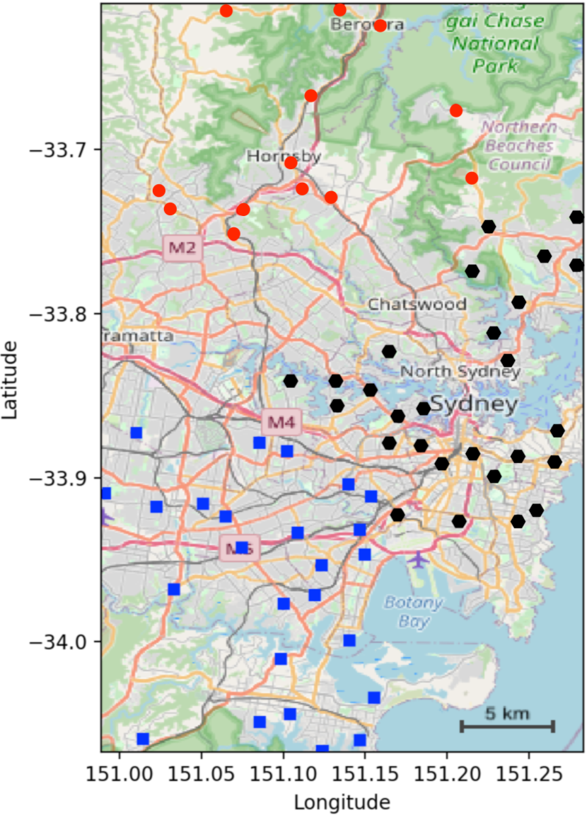
Figure 2. The approximate locations of customers in Ausgrid dataset. The unit of scale bar is 5 km.

5.1. Datasets

We use two publicly available datasets, namely Pecan Street (Pecan Street Inc., [n.d.]) and Ausgrid (Ausgrid, [n.d.]), to evaluate the estimation accuracy of different solar disaggregation methods. Both datasets include net load measurements in addition to direct measurements of home load and solar generation from homes with rooftop PV systems.

Pecan Street dataset: This dataset contains customer-level measurements of solar generation and appliance loads from homes that are located in different cities in New York, California, and Texas. Since the target home and solar proxies need to be in the same city, we restrict our focus to 19 homes that are located in Austin, Texas (in the northern hemisphere), and have solar generation and home load data. We set the latitude and longitude of all PV systems to 30.292432 and -97.699662, which are the coordinates of a randomly selected location in Austin. We collect 15-minute interval data from each home over two time periods, one in the summer and one in the winter. Specifically, the summer period ($T$=2880) is from June 1, 2018 to June 30, 2018 and the winter period ($T$=2688) is from December 3, 2018 to December 30, 2018.

Ausgrid dataset: This dataset consists of 150 customers with rooftop PV systems in Sydney, Australia (in the southern hemisphere) with the latitude and longitude of -33.888575 and 151.187349 respectively. Figure 2 shows the locations of these customers. These locations are approximate since we only have the postal code of each customer. It is also likely that a marker in this figure represents multiple customers that have the same postal code. Since Sydney is a sprawling city, we cluster the customers into three clusters according to their latitude and longitude. Points within each cluster are drawn in the same color and shape in Figure 2. As it can be seen, each cluster still spans a large area of the city. Unlike the data obtained from Pecan Street, the solar generation and home load in this dataset are sampled at 30-minute intervals. We consider two periods in two seasons, one from November 1, 2012 to November 30, 2012 in the summer season ($T$=1440) and the other one from May 1, 2013 to May 30, 2013 in the winter season ($T$=1440). A small number of customers are removed due to data quality issues in each season.

Weather data: For the city of Austin, we acquire solar radiation, wind speed, and outside air temperature from the National Solar Radiation Database (Laboratory, [n.d.]). This gives us one reading every 30 minutes. To match the temporal resolution of the load data, we use linear interpolation to upsample the weather data (to one reading every 15 minutes). For the city of Sydney in Australia, we pull in the respective weather and irradiance data with 30-minute temporal resolution using the Solcast API (Solcast, [n.d.]). The load data has the same temporal resolution in this case.

5.2. Variants of our Disaggregation Method

Table 1. Physical parameters of synthetic proxies in different proxy settings.

	orientation (∘)		tilt (∘)		DC rating (kW)
Method	Pecan	Ausgrid	Pecan	Ausgrid	Pecan	Ausgrid
1P+1SP(SP1)	180	0	30.3	33.9	3	3
1P+3SP(SP1)	180	0	30.3	33.9	3	3
1P+3SP(SP2)	90	90	30.3	33.9	3	3
1P+3SP(SP3)	270	270	30.3	33.9	3	3

1P+3SP(SPx) refers to the $x^{\text{th}}$ synthetic proxy in 1P+3SP; The panel faces respectively N, E, S, and W when the orientation angle is $0^{\circ}$, $90^{\circ}$, $180^{\circ}$, $270^{\circ}$.

We implement our method with 4 different solar proxy settings.

• 3Proxies: we directly use solar generation data for the same periods from 3 real rooftop PV systems in the same city.

• 1P+1SP: we only use 1 real solar proxy combined with 1 synthetic proxy. In this case, the ideal orientation angle in each hemisphere is used to create the synthetic proxy. It is specifically $180^{\circ}$ in the northern hemisphere and $0^{\circ}$ in the southern hemisphere.

• 1P+3SP: we use 1 real solar proxy combined with 3 synthetic proxies with different orientation angles.

• 3SP: we use 3 synthetic proxies with different orientation angles just like the previous setting.

The parameters for different synthetic proxies are shown in Table 1. We set the tilt angle to the absolute value of the city’s latitude and use a uniform DC rating for all synthetic proxies. The tilt and DC rating have a similar effect on solar generation curve, i.e., they scale the curve up or down (Chen et al., 2017), whereas the orientation shifts the peak of the generation curve to earlier or later. Therefore, we can set the tilt angle and DC rating similarly for all the synthetic solar proxies because the elements of our weight vector w will be adjusted by Algorithm 1.

5.3. Baselines

We compare the performance of our solar disaggregation method with two methods that also use the data that is commonly available to the utility and outperform other solar disaggregation methods proposed in the literature. Specifically, we use the solar disaggregation methods proposed in (Kabir et al., 2019) and (Bashir et al., 2019) as our baselines; these methods are labelled “Baseline 1” and “Baseline 2”, respectively. For a fair comparison, we implement the one-nearby-proxy-based solar estimation method in (Bashir et al., 2019) that was adopted in the case study of computing the clear sky index. In each experiment, we use the same real solar proxy for our method and Baseline 2. It is worth mentioning that in some homes the PV system’s physical characteristics estimated by Baseline 2 can be quite different from their true values due to the inaccuracy of location information and lack of directly measured solar generation from the respective homes. Therefore, in our implementation of Baseline 2 we constrain the system’s orientation within specific bounds based on the hemisphere in which the home is located.

5.4. Evaluation Metrics

We use two metrics to assess the performance of our disaggregation method with different proxies, and compare them with the two baselines. The first metric is the root-mean-square error (RMSE) which has been used in many solar disaggregation papers. The second one is a normalized RMSE metric, called nRMSE. Equation (6) is the definition of nRMSE for the estimated solar generation of a customer. It is the RMSE normalized by the mean value of the real solar generation.

(6) $$\begin{split}nRMSE&=\frac{\sqrt{\sum_{t=1}^{T}(\textbf{s}_{t}-\hat{\textbf{s}}_{t})^{2}/T}}{\sum_{t=1}^{T}\textbf{s}_{t}/T}=\frac{\text{RMSE}}{\text{Mean}}\\ \end{split}$$

Compared to RMSE, this normalized metric can help us compare the disaggregation performance on signals with different magnitudes (i.e., generation from PV panels with different sizes).

Table 2. Comparison of various disaggregation methods. Each cell contains two slash-separated metrics: nRMSE and RMSE.

	Summer				Winter
	Ausgrid		Pecan		Ausgrid		Pecan
Method	Solar	Load	Solar	Load	Solar	Load	Solar	Load
3Proxies	0.469/0.0621	0.232/0.0593	0.357/0.359	0.157/0.353	0.771/0.0602	0.199/0.0582	0.300/0.142	0.164/0.136
1P+1SP	0.543/0.0723	0.273/0.0686	0.484/0.489	0.211/0.474	0.841/0.0677	0.226/0.0649	0.375/0.179	0.211/0.175
1P+3SP	0.525/0.0691	0.254/0.0650	0.510/0.515	0.223/0.500	0.797/0.0638	0.212/0.0617	0.336/0.161	0.189/0.158
3SP	0.643/0.0858	0.305/0.0780	0.604/0.610	0.259/0.581	0.854/0.0702	0.231/0.0669	0.420/0.204	0.239/0.198
Baseline 1	0.612/0.0778	0.287/0.0778	0.516/0.493	0.221/0.493	1.713/0.1210	0.375/0.1210	0.516/0.254	0.284/0.254
Baseline 2	0.631/0.0857	0.337/0.0857	0.518/0.478	0.224/0.478	0.927/0.0767	0.272/0.0767	0.508/0.232	0.280/0.232

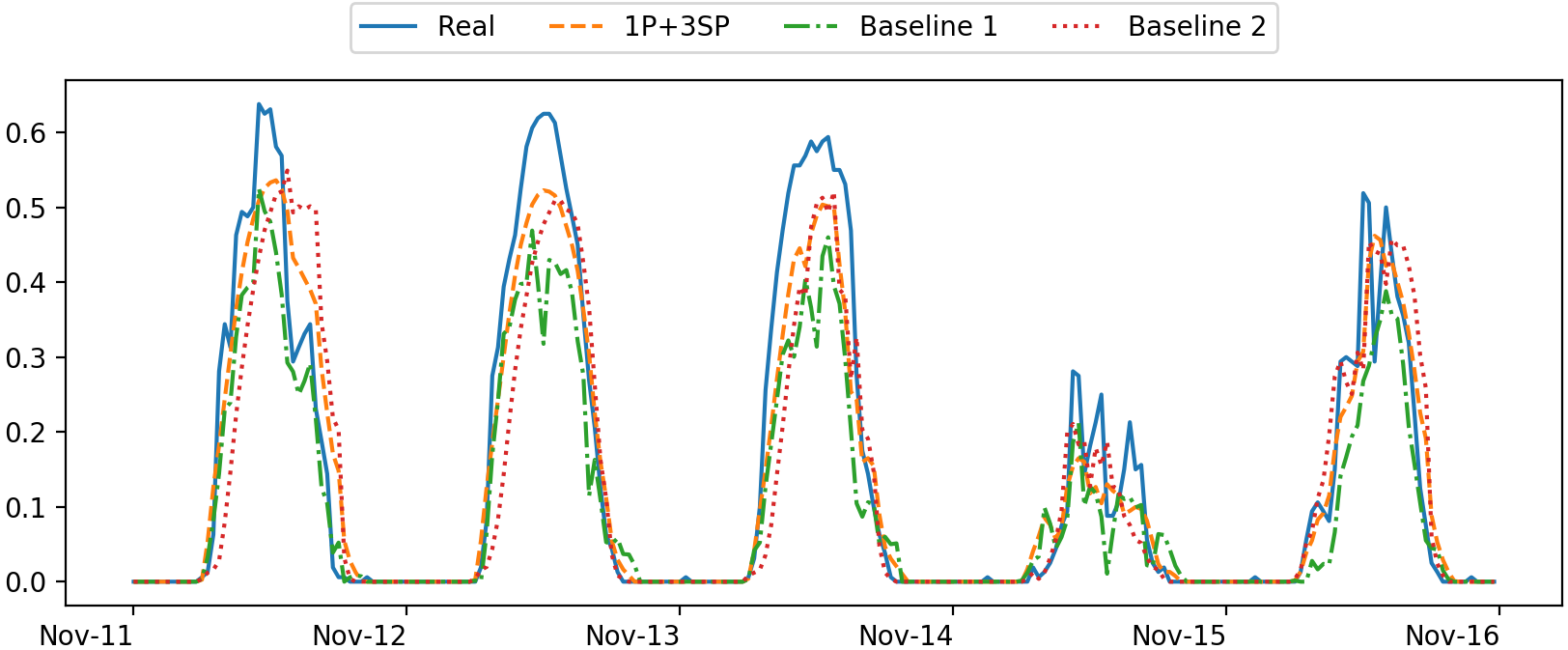
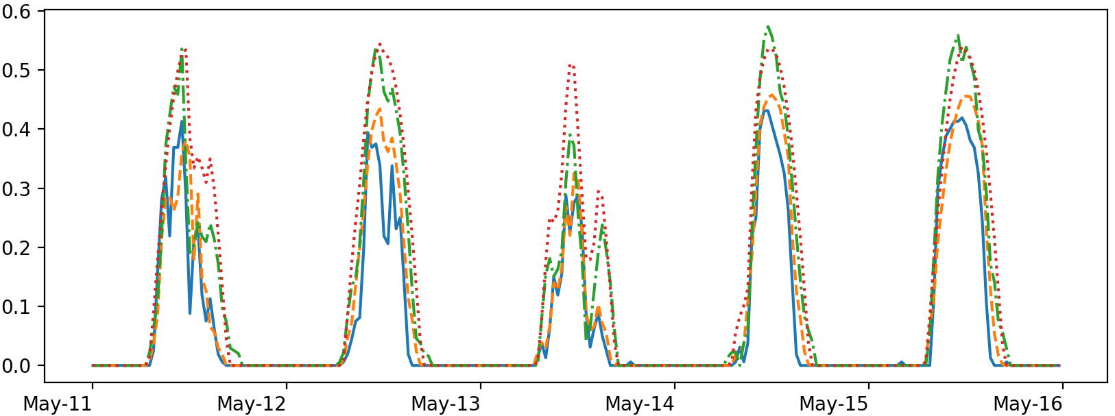
Figure 3. Comparison of disaggregated solar generation in summer (top) and winter (bottom) for a customer.

6. Experimental Results

We first evaluate the performance of our methods in disaggregating BTM solar generation using the metrics introduced in the previous section. We analyze the sensitivity of our methods to the amount of net meter data used for disaggregation, the choice of solar proxies, and the weight initialization method. Lastly, we investigate the impact of running NILM methods on the disaggregated solar generation, real solar generation, and net load. This will reveal the potential benefits of disaggregating solar generation prior to performing NILM.

Figure 4. The distribution of nRMSE values for the estimated solar generation in Ausgrid (left column) and Pecan Street (right column) datasets. The legend shows the solar disaggregation methods shown in each panel (from left to right). The length of the whiskers is 1.5 times IQR.

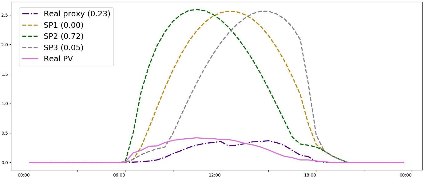
Figure 5. PV generation (kW) of a sample home. Dashed curves show proxy measurements. The relative weights (normalized to sum to 1) of proxies are put in the legend.

6.1. Solar Disaggregation Performance

We compare 4 variants of our method – 3Proxies, 1P+1SP, 1P+3SP, and 3SP – with the two baselines described in Section 5.2. For each variant, we evaluate the disaggregation performance for all customers with PV systems in the dataset. Since our method utilizes proxy measurements, we run the experiment 10 times for each target home with real solar proxies that are randomly selected from the pool (excluding the target home). For the Ausgrid dataset, we select real solar proxies from the same cluster as the target home (shown in Figure 2).

Estimation accuracy: Table 2 shows the average nRMSE and RMSE of solar generation and home load estimation across all customers in two seasons and two different datasets. We observe that 3Proxies yields the lowest error compared to the other variants of our method and the two baselines. 1P+1SP outperforms the two baselines in both seasons, reducing nRMSE by 29.74% and 12.14% on average, respectively. Similarly, 1P+3SP outperforms the two baselines in all cases except summer in the Pecan the Street dataset; in this case, Baseline 1 and Baseline 2 have comparable performance to 1P+3SP. Specifically, 1P+3SP has lower nRMSE for solar estimation, while Baseline 1 and Baseline 2 have lower RMSE (on average) for solar and load estimation. Overall, 1P+3SP reduces nRMSE of solar estimation by 32.31% and 15.66% on average compared to Baseline 1 and Baseline 2, respectively. This observation suggests that by utilizing as few as only one directly measured solar generation site, we can get a better estimate of solar generation and home load than the state-of-the-art solar disaggregation methods. Interestingly, 3SP has the worst performance among the four variants of our method, although it still beats Baseline 1 and Baseline 2 in winter. This underscores the importance of having at least one real proxy for solar disaggregation to account for high frequency variations (e.g., due to a passing cloud) in the solar generation. We do not consider 3SP in the next section for sensitivity analysis as it does not use a real proxy.

Figure 3 illustrates the disaggregated solar generation in two seasons by 1P+3SP and the two baseline methods for a randomly selected home from the Ausgrid dataset. It can be seen that our estimated solar is generally closer to true solar generation in terms of estimating peak generation time and generation scale. Figure 4 shows box and whisker plots indicating the nRMSE distribution for each disaggregation method. All the methods have relatively small variances in the Pecan Street dataset, though the variances are noticeably larger for the Ausgrid dataset, especially in winter where there are several outliers. It can be seen that our method (1P+3SP) outperforms both baselines for most homes. In a small number of homes, its performance is on par with Baseline 2 that also utilizes proxy solar measurements from a neighbouring site. This suggests that using synthetic proxies in addition to the real proxy improves the estimation accuracy in most cases.

Figure 5 shows real solar generations of a target home besides the four proxy measurements used in 1P+3SP. It can be seen that the peak generation of the target home and real solar proxy happen at different times as they have different orientations. In this case, the synthetic proxy with an orientation angle close to the target home’s orientation angle gets a much higher weight compared to the other synthetic proxies and the real proxy. This highlights the advantage of incorporating the synthetic proxies.

Computation time: We now compare our method (the 1P+3SP variant) with the baselines in terms of their running time. Excessively high running times could be prohibitively costly for the utilities that intend to run the solar disaggregation method at scale. We use an Intel Xeon Silver 4114 CPU to run the experiments. The total running time for disaggregating one month data from a target home in Ausgrid using 1P+3SP is around 35 seconds (25 seconds for weight initialization and 10 seconds for solar disaggregation). The other variants of our method have similar running times. In comparison, the total running time of Baseline 1 is about 70 minutes, which is roughly 120 times greater than the running time of our method. We attribute this to the fact that this method solves a nonlinear optimization problem for the solar model and trains a Markov switching regression model for load estimation in every iteration. Although Baseline 2 has a running time that is similar to our proposed method (i.e., 30 seconds), its estimation accuracy is worse than ours as explained in the previous section.

6.2. Sensitivity Analysis

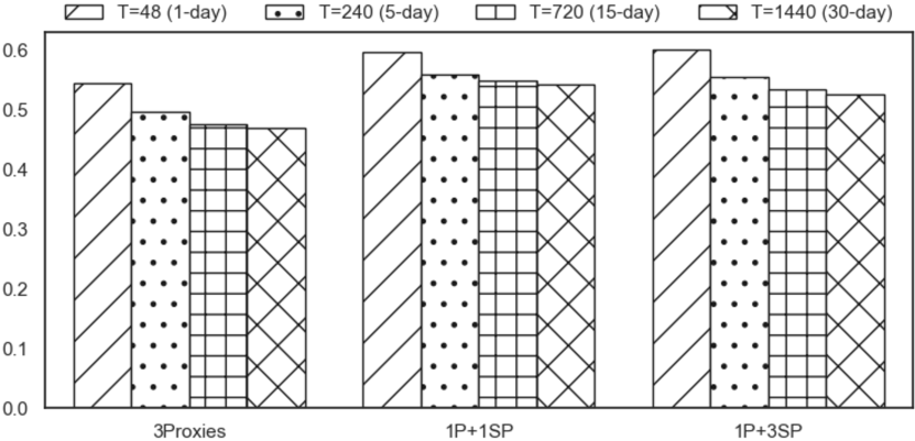
Figure 6. nRMSE of disaggregated solar for different disaggregation lengths in the Ausgrid dataset.

Disaggregation length: We now investigate how extending the length of solar generation data would impact the performance of our disaggregation method. We set the disaggregation length $T$ to be {48, 240, 720, 1,440} time intervals corresponding to {1, 5, 15, 30} days of data from Ausgrid. Then, we apply our method to each $T$ consecutive intervals separately. Similar to the implementation in the previous subsection, we run 10 independent experiments and average the error values for each target home to account for the randomness caused by choosing different solar proxies. Figure 6 shows the nRMSE of 3Proxies, 1P+1SP, and 1P+3SP for different disaggregation length. For all three variants, the nRMSE is larger for shorter disaggregation periods. This could be because more data is available for longer periods, which is helpful to capture the true relationship between the solar generation of the target home and solar proxies.

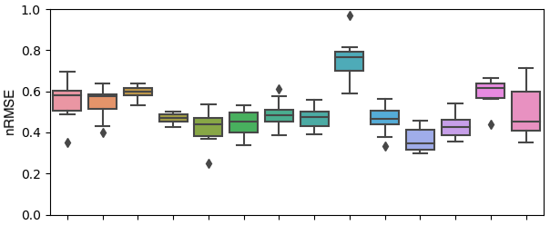
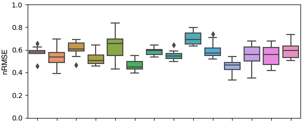
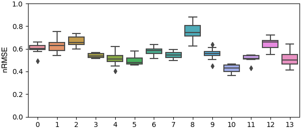
Figure 7. The distribution of nRMSE values obtained using different choices for the proxy measurement. The top plot shows the results from 3Proxies, the middle plot shows the results from 1P+1SP, and the bottom one shows the results from 1P+3SP. The x-axis indicates the home index.

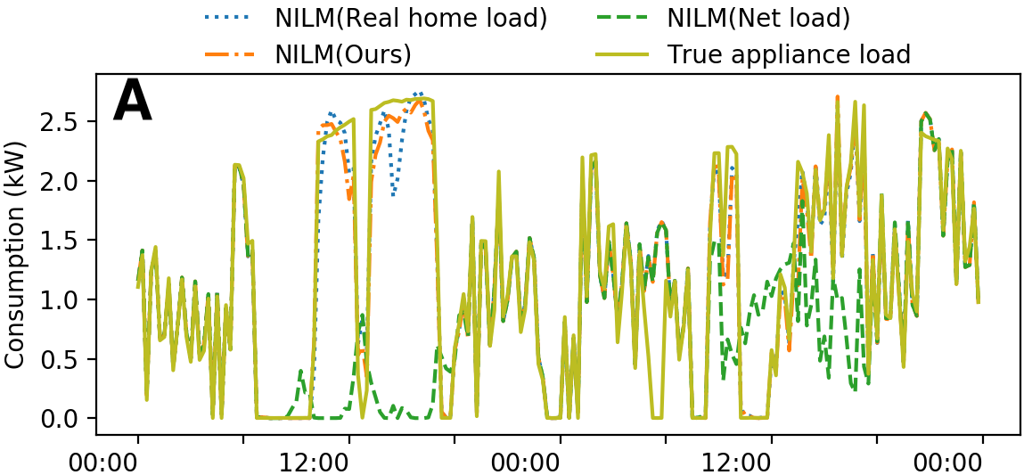
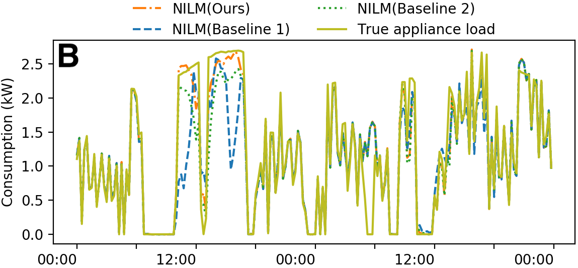
Figure 8. Comparison between the true and estimated air conditioner (AC) loads. The top plot shows the results of running Seq2Point on real home load, net load, and the home load disaggregated by our method (1P+3SP). The bottom plot shows the results of running Seq2Point on the home load disaggregated by our method (1P+3SP) and 2 baselines.

Selection of solar proxies: To evaluate the sensitivity of our methods to the choice of solar proxies, we randomly choose 14 target homes in Ausgrid and run 10 independent experiments with solar proxies that are randomly chosen in each experiment. Figure 7 shows the nRMSE distribution for the 14 different target homes. It can be seen that the nRMSE distributions obtained for a few target homes are wider than the rest, implying that the disaggregation method is more sensitive to the choice of solar proxies. This is because these homes are located far from the majority of homes in this dataset. Expectedly, 1P+3SP is the least sensitive variant to the choice of solar proxy because it only requires one real solar proxy and incorporates three synthetic proxies.

Table 3. Comparing nRMSE of disaggregated solar using different methods to initialise the weight vector w.

	Constant	Random	Ours
3Proxies	0.78553	1.49346	0.46856
1P+1SP	2.80917	2.93639	0.54347
1P+3SP	3.80280	8.85139	0.52521

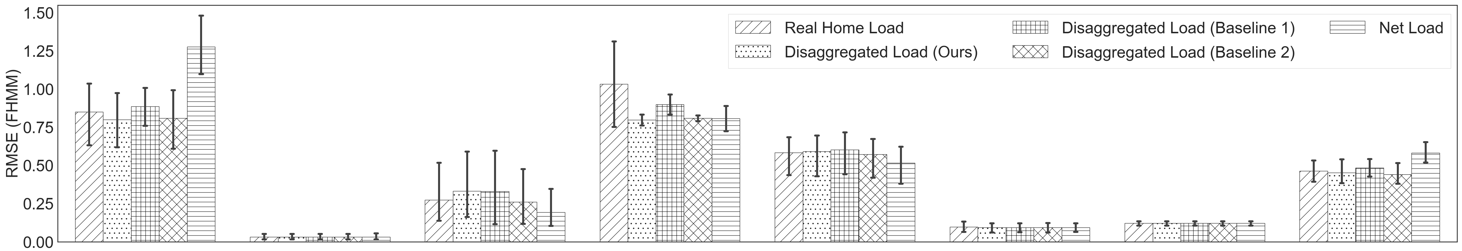
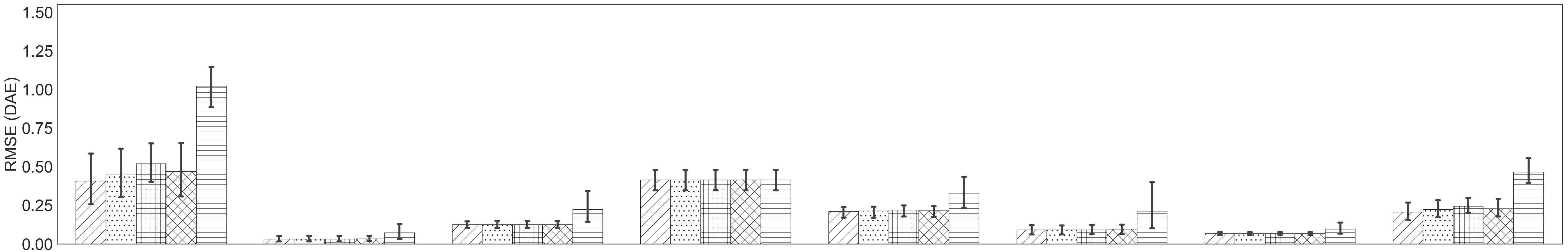
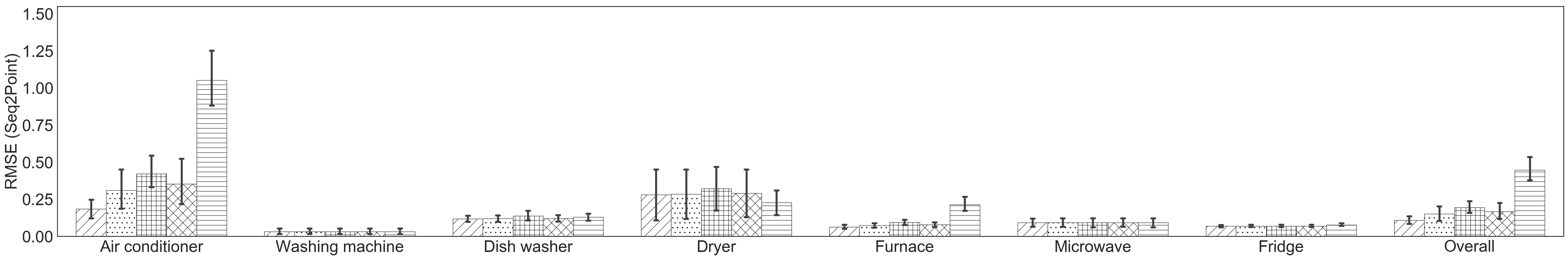
Figure 9. Average RMSE of each appliance among all selected homes. The top plot shows the disaggregation performance of FHMM, the middle plot shows the performance of DAE, and the bottom one shows the performance of Seq2Point. Error bars show the 95% confidence interval.

Weight initialization: To evaluate the efficacy of our initialization method, we compare it with constant and random initialization methods. We simply set w to $\mathbf{1}$ for constant initialization. For random initialization, we assign random numbers in the range of $[0,1]$ to the weights. Table 3 compares the results. It is evident that our weight initialization method can significantly increase the accuracy of solar disaggregation, especially when we use only one real solar proxy (i.e., 1P+1SP and 1P+3SP). We attribute this to the fact that we take into account the PV system deployment characteristics estimated by SolarTK.

6.3. NILM Performance

We study the effect of BTM solar generation on the performance of NILM techniques. For the purpose of this study, we select 6 homes from the Pecan Street dataset that have both solar generation and individual appliance consumption data, and apply three benchmark NILM techniques, namely FHMM (Kim et al., 2011), Seq2Point (Zhang et al., 2018), and DAE (Kelly et al., 2015). These techniques are implemented in NILMTK (Batra et al., 2019). Following the recommendation of (Huchtkoetter et al., 2020), which explored the impact of the temporal resolution of data on the accuracy of NILM methods, we use data with 1-minute resolution.

We evaluate the performance of these 3 NILM methods in disaggregating the loads of 7 appliances, including the washing machine, microwave, air conditioner, furnace, fridge, dryer and dish washer, in each of the 6 homes. Since a dryer is not present in 4 of these homes, we only report the results for the remaining 2 homes for this appliance. We train appliance models using real home load and individual appliance load data collected between June 1 and June 22, 2018. We then calculate the error of disaggregating each appliance’s load in the test data (from June 23 to June 30, 2018) with 5 different sets of input data, including the true home load, the net load (i.e., home load - BTM solar generation), and 3 versions of the disaggregated home load obtained by applying our disaggregation method (1P+3SP), and the two baseline methods described earlier.

Figure 9 shows the average RMSE for each appliance and the overall RMSE for all appliances in these homes. Two important observations can be made. First, solar disaggregation will improve the overall NILM accuracy but different appliances are affected to a different extent. The overall RMSE for all appliances will be 0.446 if we directly apply Seq2Point (the best performing NILM method) on the net load data. However, the RMSE will be 0.150 if we apply it to the disaggregated home load estimated by 1P+3SP, an impressive 66.2% improvement in disaggregation accuracy. We also observed 52.3% and 22.0% improvements for DAE and FHMM methods, respectively. Among all appliances, the air conditioner shows the most significant improvement in accuracy, while the disaggregation accuracy of the washing machine, dryer, microwave, and dish washer does not exhibit a statistically significant change. This may be due to the fact that these appliances are usually used after the sunset, when the net load is equal to the home load, while the air conditioner is used throughout the day. It is also worth mentioning that the fridge yields quite similar performance for all 5 different types of input data using the 3 NILM techniques. Our hypothesis is that this is because the fridge has a distinct power consumption pattern that is easier to detect.

Our second observation is that a higher accuracy in solar disaggregation leads to a better NILM performance, especially for appliances with more variable power usage patterns (e.g., the air conditioner). The overall RMSE of Seq2Point when it runs on the disaggregated home load obtained by the 1P+3SP method is 22.3% and 9.7% lower than when it runs on the disaggregated home load obtained by applying Baseline 1 and Baseline 2, respectively. Among the 7 appliances, the NILM performance improvement achieved by our method over the two baselines is particularly noticeable for air conditioner, which is the most power-hungry appliance in our study.

From the results depicted in Figure 9 it is clear that Seq2Point yields a better performance than the other 2 NILM methods. To further study the effect of solar disaggregation on the the performance of NILM, we compare the air conditioning load obtained by applying Seq2Point to the net load, true home load, and disaggregated home load using our 1P+3SP method in Figure 8(A). We also show the true air conditioning load as a point of reference. We can see that the error of directly applying Seq2Point to the net load data is specially high around noon which solar generation is usually at its peak. Figure 8(B) compares the air conditioner load obtained by applying Seq2Point to the home load disaggregated by 1P+3SP and the 2 baselines. It can be seen that among the three solar disaggregation methods, our method enables tracking the true air conditioner’s demand more closely.

7. Conclusion

Solar disaggregation will be essential for the reliable operation of a nimble and transparent power distribution system. We proposed a method for disaggregating solar generation of BTM PV systems in an offline fashion. This method relies on net load data and proxy measurements from a few solar PV systems located in the same geographic area as the target home. We evaluated our proposed method on two different dataset from two countries with different climates. We found that the solar estimation accuracy improves by 15.66% on average over the best baseline (i.e., Baseline 2) when one real proxy and three synthetic proxies are used. Finally, we investigated whether a more accurate disaggregation technique could lead to higher accuracy in NILM. Our results suggest that using the disaggregated home load rather than the net load improves the overall accuracy of NILM by 22.0% to 66.2%.

There are several avenues for future work. First, we plan to test our method in a different climate where snow accumulation can greatly affect the output of PV systems. We will explore how the proposed solar disaggregation technique can be used to estimate and predict the total amount of solar power generated in a neighbourhood. Another interesting direction that will be pursued is to design a solar disaggregation method that can be used in the presence of BTM battery storage.

References

- (1)
- Ausgrid ([n.d.]) Ausgrid. [n.d.]. Solar home electricity data. https://www.ausgrid.com.au/Industry/Our-Research/Data-to-share/Solar-home-electricity-data.
- Bashir et al. (2019) Noman Bashir et al. 2019. Solar-TK: A Data-Driven Toolkit for Solar PV Performance Modeling and Forecasting. In Proc. 16th International Conference on Mobile Ad Hoc and Sensor Systems (MASS). IEEE, 456–466.
- Batra et al. (2019) Nipun Batra et al. 2019. Towards Reproducible State-of-the-Art Energy Disaggregation. In Proc. 6th International Conference on Systems for Energy-Efficient Buildings, Cities, and Transportation. ACM, 193–202.
- Bu et al. (2020a) Fankun Bu et al. 2020a. A Data-Driven Game-Theoretic Approach for Behind-the-Meter PV Generation Disaggregation. IEEE Transactions on Power Systems 35, 4 (2020), 3133–3144.
- Bu et al. (2020b) Fankun Bu et al. 2020b. Disaggregating Customer-level Behind-the-Meter PV Generation Using Smart Meter Data. arXiv (2020), 1–8.
- Chen et al. (2017) Dong Chen et al. 2017. SunDance: Black-box Behind-the-Meter Solar Disaggregation. Proc. 8th International Conference on Future Energy Systems (2017), 45–55.
- Chen et al. (2020) Xinlei Chen et al. 2020. Solar Disaggregation: State of the Art and Open Challenges. In Proc. 5th International Workshop on Non-Intrusive Load Monitoring. ACM, 6–10.
- Cheung et al. (2018) Chung M. Cheung et al. 2018. Behind-the-Meter Solar Generation Disaggregation using Consumer Mixture Models. In International Conference on Communications, Control, and Computing Technologies for Smart Grids. IEEE, 1–6.
- Chueng et al. (2020) Chung M. Chueng et al. 2020. Disaggregation of Behind-the-Meter Solar Generation in Presence of Energy Storage Resources. In Conference on Technologies for Sustainability (SusTech). IEEE.
- de Hoog et al. (2020) Julian de Hoog et al. 2020. Using Satellite and Aerial Imagery for Identification of Solar PV: State of the Art and Research Opportunities. In Proc. 11th International Conference on Future Energy Systems. ACM, 308–313.
- Dinesh et al. (2017) Chinthaka Dinesh et al. 2017. Non-intrusive load monitoring under residential solar power influx. Applied Energy 205 (2017), 1068–1080.
- Dobos (2014) Aron Dobos. 2014. PVWatts Version 5 Manual. Technical Report. Research Organization: National Renewable Energy Lab. (NREL), Golden, CO (United States).
- Gu-yuan Lin et al. (2010) Gu-yuan Lin et al. 2010. Applying power meters for appliance recognition on the electric panel. In Proc. 5th Conference on Industrial Electronics and Applications. IEEE, 2254–2259.
- Hart (1992) George W. Hart. 1992. Nonintrusive appliance load monitoring. Proc. IEEE 80, 12 (1992), 1870–1891.
- Huchtkoetter et al. (2020) Jana Huchtkoetter et al. 2020. On the Impact of Temporal Data Resolution on the Accuracy of Non-Intrusive Load Monitoring. In Proc. 7th International Conference on Systems for Energy-Efficient Buildings, Cities, and Transportation. ACM, 270–273.
- International Energy Agency (2020) International Energy Agency. 2020. Global Energy Review 2020. https://www.iea.org/reports/global-energy-review-2020. Accessed 01.02.2021.
- Kabir et al. (2019) Farzana Kabir et al. 2019. Estimation of Behind-the-Meter Solar Generation by Integrating Physical with Statistical Models. In IEEE International Conference on Communications, Control, and Computing Technologies for Smart Grids. 1–6.
- Kabir et al. (2021) Farzana Kabir et al. 2021. Joint Estimation of Behind-the-Meter Solar Generation in a Community. IEEE Transactions on Sustainable Energy 12, 1 (2021), 682–694.
- Kara et al. (2018) Emre Kara et al. 2018. Disaggregating solar generation from feeder-level measurements. Sustainable Energy, Grids and Networks 13 (2018), 112–121.
- Kelly et al. (2015) Jack Kelly et al. 2015. Neural NILM: Deep Neural Networks Applied to Energy Disaggregation. Proc. 2nd ACM International Conference on Embedded Systems for Energy-Efficient Built Environments (2015).
- Kim et al. (2011) Hyungsul Kim et al. 2011. Unsupervised Disaggregation of Low Frequency Power Measurements. Proc. SIAM Conference on Data Mining 11, 747–758.
- Kukunuri et al. (2020) Rithwik Kukunuri et al. 2020. EdgeNILM: Towards NILM on Edge Devices. In Proc. 7th International Conference on Systems for Energy-Efficient Buildings, Cities, and Transportation. ACM, 90–99.
- Laboratory ([n.d.]) The National Renewable Energy Laboratory. [n.d.]. National solar radiation database. https://nsrdb.nrel.gov/.
- Mauch et al. (2016) Lukas Mauch et al. 2016. A novel DNN-HMM-based approach for extracting single loads from aggregate power signals. In International Conference on Acoustics, Speech and Signal Processing (ICASSP). IEEE, 2384–2388.
- OpenStreetMap contributors (2017) OpenStreetMap contributors. 2017. Planet dump retrieved from https://planet.osm.org . https://www.openstreetmap.org.
- Pecan Street Inc. ([n.d.]) Pecan Street Inc. [n.d.]. Dataport. https://www.pecanstreet.org/dataport/.
- Pedregosa et al. (2011) Fabian Pedregosa et al. 2011. Scikit-learn: Machine learning in Python. Journal of Machine Learning Research 12, Oct (2011), 2825–2830.
- Shaker et al. (2016a) Hamid Shaker et al. 2016a. A Data-Driven Approach for Estimating the Power Generation of Invisible Solar Sites. IEEE Transactions on Smart Grid 7, 5 (2016), 2466–2476.
- Shaker et al. (2016b) Hamid Shaker et al. 2016b. Estimating Power Generation of Invisible Solar Sites Using Publicly Available Data. IEEE Transactions on Smart Grid 7, 5 (2016), 2456–2465.
- Shi et al. (2019) Xin Shi et al. 2019. Nonintrusive load monitoring in residential households with low-resolution data. Applied Energy 252 (2019), 113283.
- Singh et al. (2020) Shikha Singh et al. 2020. Compressive Non-Intrusive Load Monitoring. In Proc. 7th International Conference on Systems for Energy-Efficient Buildings, Cities, and Transportation. ACM, 290–293.
- Solcast ([n.d.]) Solcast. [n.d.]. Weather Dataset. https://toolkit.solcast.com.au/.
- Sossan et al. (2018) Fabrizio Sossan et al. 2018. Unsupervised Disaggregation of Photovoltaic Production From Composite Power Flow Measurements of Heterogeneous Prosumers. IEEE Transactions on Industrial Informatics 14, 9 (2018), 3904–3913.
- Stein (2012) Joshua Stein. 2012. The Photovoltaic Performance Modeling Collaborative (PVPMC). In 38th Photovoltaic Specialists Conference. IEEE, 003048–003052.
- Tabone et al. (2018) Michaelangelo Tabone et al. 2018. Disaggregating Solar Generation behind Individual Meters in Real Time. In Proc. 5th Conference on Systems for Built Environments. ACM, 43–52.
- Völker et al. (2020) Benjamin Völker et al. 2020. FIRED: A Fully-Labeled HIgh-FRequency Electricity Disaggregation Dataset. In Proc. 7th International Conference on Systems for Energy-Efficient Buildings, Cities, and Transportation. ACM, 294–297.
- Wang et al. (2020) Shuangyuan Wang et al. 2020. Regional nonintrusive load monitoring for low voltage substations and distributed energy resources. Applied Energy 260 (2020), 114225.
- Zhang et al. (2018) Chaoyun Zhang et al. 2018. Sequence-to-Point Learning With Neural Networks for Non-Intrusive Load Monitoring. In AAAI.