X-ray Observations of 1ES 1959+650 in its high activity state in 2016-2017 with AstroSat and Swift

Abstract

We present a comprehensive multi-frequency study of the HBL 1ES 1959+650 using data from various facilities during the period 2016-2017, including X-ray data from AstroSat and Swift during the historically high X-ray flux state of the source observed until February 2021. The unprecedented quality of X-ray data from high cadence monitoring with the AstroSat during 2016-2017 enables us to establish a detailed description of X-ray flares in 1ES 1959+650. The synchrotron peak shifts significantly between different flux states, in a manner consistent with a geometric (changing Doppler factor) interpretation. A time-dependent leptonic diffusive-shock-acceleration and radiation transfer model is used to reproduce the spectral energy distributions (SEDs) and X-ray light curves, to provide insight into the particle acceleration during the major activity periods observed in 2016 and 2017. The extensive data of Swift-XRT from December 2015 to February 2021 (Exp. = 411.3 ks) reveals a positive correlation between flux and peak position.

1 Introduction

Blazars are a subclass of active galactic nuclei (AGN) with a jet of relativistic plasma streaming along or very close to the line of sight (Blandford & Rees, 1978). The observed electromagnetic (EM) emission, which is predominantly non-thermal in nature, is considered to be emanating from the relativistic jet. The observed features of blazars include superluminal motion of radio-jet components, high optical polarisation and strong continuum emission variable at time scales ranging from a few minutes to years, across the entire EM spectrum.

The broadband spectral energy distribution (SED; $\nu$ v/s $\nu$F_ν plot) of blazars consists of two distinct broad continuum hump like structures with the first one peaking somewhere in sub-mm to soft X-rays, whereas the second one peaks at MeV to TeV energies (Urry & Padovani, 1995). The low-energy component of the SED is mostly due to the synchrotron emission from relativistic electrons/positrons gyrating around the magnetic field in the relativistic jet. This emission component, in some cases, is superimposed by significant thermal contributions from, e.g., the accretion disk, a hot corona accompanying the accretion disk, and/or an obscuring dusty torus. On the other hand, the physical mechanisms behind high energy emission (MeV to TeV) are not well established and two families of models namely, a) leptonic models, and, b) hadronic models, both appear to be viable mechanisms to explain the X-ray through $\gamma$-ray emission. In hadronic models the high energy emission is produced by relativistic protons through proton synchrotron radiation and photo-pion production, followed by pion decay and electromagnetic cascades (e.g., Mannheim & Biermann, 1992; Nellen et al., 1993; Mannheim, 1993; Protheroe & Mücke, 2001; Mücke et al., 2003; Böttcher et al., 2013a). Leptonic models assume the jet protons to be cold enough not to contribute to the radiative output, and high-energy emission is produced by inverse Compton scattering of low energy seed photons by the ultra-relativistic leptons (e^-/e⁺). The seed photons may come from the synchrotron radiation field in the emission region, which are up-scattered by the same leptons that produced the synchrotron radiation (Synchrotron Self-Compton = SSC) (Ghisellini & Maraschi, 1989; Bloom & Marscher, 1996; Mastichiadis & Kirk, 1997)). Alternatively, if the seed photons originate external to the emission region (e.g., from the accretion-disk, the dusty torus, or the broad-line region) then the process is termed as External Compton (EC). (Dermer et al., 1992; Ghisellini et al., 1998)).

1ES 1959+650 ($z=0.048$; Perlman et al., 1996) is a prominent high-synchrotron-peaked blazar. It was first detected in X-rays during the Slew Survey with the Einstein Imaging Proportional Counter (IPC) (Elvis et al., 1992), followed by BeppoSAX (Beckmann et al., 2002), RXTE, Swift, XMM-Newton (Tagliaferri et al., 2003; Massaro et al., 2008) in later years. This source is also a prominent TeV $\gamma$-ray emitter, with the first detection at TeV energies, reported by the Utah Seven-Telescope Array collaboration in 1998 (Nishiyama, 1999).

The historical observations establish 1ES 1959+650 to be a High-frequency peaked BL Lac object (HBL) in which the synchrotron peak of the broadband SED appears in UV – X-ray band (Krawczynski et al., 2004a; Kapanadze et al., 2016a; Abdo et al., 2010). This source exhibits strong flux variability across almost the entire EM spectrum. The flux increase of up to 3-4 orders of magnitude in the optical, X-ray, and TeV energy bands during the short/erratic flares have been witnessed for 1ES 1959+650 (Perlman et al., 2005; Krawczynski et al., 2004a; Kapanadze et al., 2016b). The rapid variability and its frequency dependence provide crucial insight into the physical processes of particle acceleration and radiation mechanisms as well as the geometry and size of the emission region (e.g., Dondi & Ghisellini, 1995).

Recent high-sensitivity X-ray observations have found several high flux states and strong X-ray outbursts of this source. XMM-Newton and RXTE-PCA observations in 2002 – 2003 revealed strong X-ray flares with flux variations by a factor up to $\sim$ 4.2 (Perlman et al., 2005; Krawczynski et al., 2004a). Many of such frequently occurring strong X-ray flares were reported by Kapanadze et al. (2016b) during 2006 – 2014 using Swift-XRT observations. The source underwent a number of active states and an unprecedented X-ray flaring activity during August 2015 – January 2016 that was observed by Swift-XRT. The observed count rate was reported to vary by a factor of $\sim$5.7 with maximum value above 20 cts/s, with simultaneous high flux activity in TeV energy band (Kapanadze et al., 2016a; Kaur et al., 2017; Patel et al., 2018; MAGIC Collaboration et al., 2020). During this large flare, the synchrotron peak position of the SED showed a tendency to shift towards the higher X-ray energies accompanied by a hard X-ray spectral index. The detailed X-ray spectral studies further confirmed the harder-when-brighter trend (Tagliaferri et al., 2003; MAGIC Collaboration et al., 2020). However, during most of these epochs with an X-ray flare, the TeV counterpart was found to be in low flux states. On the other hand, in several multi-wavelength campaigns, “orphan” flares in VHE (Very High Energy, used for TeV) $\gamma$-rays (not accompanied by a simultaneous X-ray flare) have been reported in June 2002 (Krawczynski et al., 2004b) and April – June 2012 (Aliu et al., 2014).

The uncorrelated variability is inconsistent with the simplest one-zone SSC models, which are often successful in reproducing the broadband emission of HBLs, but have proven to be inadequate to explain several aspects of emission in many studies (Krawczynski et al., 2004a; Patel et al., 2018; MAGIC Collaboration et al., 2020). “Orphan” flares hint at a more complex geometry and/or underlying particle distribution, such as those invoked in multiple-component SSC models and/or external Compton models (e.g., the synchrotron mirror model, Böttcher & Dermer (1999)) within the leptonic schemes. Recently, Shah et al. (2021), have reported an anti-correlation between the photon index and X-ray flux using a broken power-law for analysing only a segment of X-ray data presented here.

In this work, we present a detailed investigation of the X-ray spectral and light curve features of 1ES 1959+650 observed by AstroSat in 2016 – 2017. Our main focus here is to understand the distinct, irregular X-ray outbursts observed during this period by both the Soft X-Ray Telescope (SXT) & Large Area Proportional Counter (LAXPC) instruments aboard AstroSat.

These data are supplemented with simultaneous/quasi-simultaneous XRT data extending before and after 2016–2017, spanning over 6 years from January 30, 2015 – February 09, 2021, and also other multi-wavelength data to probe the evolution of the underlying non-thermal particle distribution. In order to consistently fit the SEDs and the light curves obtained during these erratic flares observed with AstroSat, we adopt the time-dependent multi-zone shock acceleration and radiation transfer model, as described by Böttcher & Baring (2019), to investigate the nature of shocks responsible for the observed spectral variability. We further provide a detailed analysis of the time resolved spectra and light curves and their correlation over the span of $\sim$ 6 years.

The paper is structured as follows. Section 2 describes the multi-wavelength observation details and the data analysis procedures. In section 3, we provide the results of the timing and spectral analysis and the detailed correlation study. Section 3 contains the results and the interpretation through the modeling of snap-shot SEDs and light curves. In section 4 we summarize our work followed by a comprehensive discussion.

2 Observations and Data Analysis

1ES 1959+650 was observed in campaign mode during 2016 and 2017 at various epochs, representing different flux states, using a number of observing facilities including AstroSat, Swift, and Mt. Abu Infrared Observatory, India (MIRO). The details of the observing epochs, and the respective total exposure times are mentioned in the Table 2. PASS8 photon data from Fermi-LAT are also analysed to study the high energy (GeV) emission. The following sub-sections provide the details of the observations and analysis procedures.

Table 1: Details of the data used for the present study.

S.N.	Instrument	Total Exposure	Epoch of Observations
1	Fermi-LAT	-	57037.0 to 58072.0
2	AstroSat	143.9 ks	57666.2 - 57666.7
			57708.4 - 57709.2
			57695.9 - 57699.4
			58051.1 - 58052.6
4	Swift	411.2 ks	57052.1 - 59254.4
5	MIRO	—-	57690.81-57696.85
		R band: 8.4 hrs	”
		B band: 0.65 hrs	”
		V band: 0.65 hrs	”
6	FACT	12.4 days	57632.88-57719.83
			57997.88-58098.83

Note: MIRO: Mt. Abu Infrared Observatory, Rajasthan, India
FACT: First G-APD Cherenkov Telescope, La Palma, Spain

Table 2: Details of AstroSat observations.

S.N.	Date of Observation	Time Start/Range	SXT Exp.	LAXPC Exp.	Time-Seg.
	(UTC)	(MJD)	(ks)	(ks)
1	2015-11-20T05:28:57	57346.27	2.9	-	PV
2	2016-10-05T03:49:57	57666.2 - 57666.6	13.4	25.4	T0
3	2016-11-03T20:47:00	57695.9	82.6	147.8	F1: T1, T2, T3
					T4, T5, T6
		………….	……………..	…………….	…………….
		57695.9 - 57696.4	8.6	30.0	T1
		57696.5 - 57697.3	13.5	27.4	T2
		57697.3 - 57698.3	21.6	18.7	T3
		57698.3 - 57699.4	24.3	17.5	T4
		57696.5 - 57697.8	26.6	46.3.3	T5
		57697.8 - 57699.0	25.6	17.4	T6
		………….	……………..	…………….	…………….
4	2016-11-16T10:30:11	57708.4 - 57709.1	16.0	33.3	T7
5	2017-10-25T02:28:50	58051.1	35.1	85.7	F2: T8, T9, T10
		………….	……………..	…………….	…………….
		58051.1 - 58051.7	14.15	38.7	T8
		58051.7 - 58052.3	11.0	25.7	T9
		58052.3 - 58052.6	9.9	16.7	T10
		………….	……………..	…………….	…………….

Note: The small time segments T1-T6 and T8-T10 are used to generate time-resolved spectra to understand the various phases of flaring activities in 2016 and 2017. The time segment PV represents the first target of opportunity (ToO) observations made in 2015.

2.1 Fermi-LAT

The PASS8 (P8R3) Fermi-LAT photon data and corresponding spacecraft data from the beginning of November 2015 to the end of December 2017 are downloaded from the LAT data center with a search radius of 30 degree and in an energy range of 30 MeV to 500 GeV. The Fermitools package (version 1.2.1 conda-release) distributed by the Fermi Science Support Center, installed with the most recent release of point source (4FGL) and extended source catalogs, are used to analyse the data. The python package, fermipy(Wood et al., 2017) is used, which facilitates handy wrappers for various procedures of LAT data analysis, as described by the instrument teams, including model optimization, the localization, sanity checks and product extractions etc. The initial selection of parameters includes a bin size of 0.1 pixels for map creation, a zenith angle of accepted events of 90^∘ to exclude or eliminate most of the contamination from secondary $\gamma$-rays contributed by Earth’s limb, an energy range 100 MeV - 500 GeV, event type 3 and event class 128. The P8R3_SOURCE_V2 instrument response functions (IRFs) are used. The initial source model (XML) is created by including all the point-like and extended sources located within 25^∘ radius of the location of 1ES 1959+650 as listed in the Fourth Fermi-LAT Source catalog (4FGL Abdollahi et al., 2020), as well as the Galactic diffuse (gll_iem_v07.fits) and isotropic background emission (iso_P8R3_SOURCE_V2_v1.txt). The source model for 1ES 1959+650 imported from the 4FGL catalog is “LogParabola”; however, due to poor photon statistics for the duration of interest to this work, a re-optimization of the source model is performed after forcing the spectral shape of 1ES 1959+650 to “PowerLaw”. The spectral parameters of sources within 5^∘ of 1ES 1959+650 are kept variable while others are kept frozen to their best fit values from the catalog. TS (Test Statistics) maps and diffuse maps are generated to look for any possible GeV source (point and/or diffuse) not included in our model, but none are found. Once the model is optimized, the best fit spectral parameters for the GeV part of the SED are estimated using the sed procedure of fermipy with 2 spectral points per decade in energies. The lightcurve procedure of the fermipy package is used for generating light curves with 1 day, 2 day and 3 day binning.

The SED and light curve data points with TS $\geq$ 9 (equivalent to $\geq$ 3 $\sigma$ significance) and TS $\geq$ 25 ($\geq$ 5 $\sigma$) are used for spectral and temporal studies. For lower-significance points, 95 % upper limits are shown.

2.2 X-ray Data Analysis

The data from extensive monitoring over the course of two years using AstroSat is used for this study. Complementary data from the Neil Gehrels Swift Observatory is also used for various epochs. Table LABEL:tab:swtspec_par lists the details of the data used for this work. The general FTools and several mission specifics tools distributed as part of the heasoft package (version 6.25) and the most recent calibration database are utilized as appropriately to analyse data from various facilities.

2.2.1 AstroSat-Soft X-ray Telescope (SXT)

The SXT aboard AstroSat is a 2-m approximate Wolter-I type focusing instrument sensitive mainly in 0.3-7.1 keV energy band (Singh et al., 2014, 2016, 2017). Its camera assembly uses an e2v CCD, identical to the one flown with XMM-Newton-MOS and Swift-XRT, at its focal plane as the main detector system. The observations were carried out in photon counting mode. The source was observed throughout all the satellite orbits when the SXT was pointed at it, taking care that the Sun avoidance angle is$\geq$ 45 degrees and the RAM angle (the angle between the payload axis to the velocity vector direction of the spacecraft) $>$ 12 degrees to ensure the safety of the mirrors and the detector.

Level-2 data provided by the SXT payload operation center (POC) in Mumbai, India, are reduced using the most recent pipeline and calibration database (version 1.4b).

The level-2 cleaned events files are used in the XSELECT tool distributed with heasoft to extract source light curves, images and spectra. The clean process removed events during the occultation by the Earth, any contamination by the charged particles due to passage of the satellite through the South Atlantic Anomaly region and selected events with grade 0–12 (single-quadruple events). The filter “pha_cutoff” is applied to select various energy channels [e.g., channel 30-700 for 0.3-7.0 keV band] for the light curves.

The pile-up effect is very common for the CCD based detectors, however, due to the large PSF of the SXT, it becomes effective only for extremely bright sources like Crab or brighter (source count rate $>$ 180 s^-1). 1ES 1959+650 being only a moderately bright (max SXT count rate $\sim$ 25 s^-1, Ref. Figure 10) has no detectable pileup issue. A circular region of 16 arcmin radius around the source location, which encircles more than 95% of all photons as estimated by the standard sxtEEFmake module distributed through the POC website, is used to extract the source spectra and light curves. The appropriate ARF file suitable for the specific source region is generated using the command line auxiliary tool sxtARFModule. Because of the large point spread function (PSF) of SXT, we are unable to extract background products from the same frame and hence the background spectrum provided by the POC is used for spectral modelling. The background correction in the lightcurves corresponding to various energy bands is done by subtracting a constant which is the rate of background counts for a specific energy band normalized to the area of the source region, estimated by importing the background spectrum in XSPEC (version 12.10.1) and applying the corresponding energy filter. This background spectrum is extracted using the data from various blank-sky observations at various locations in the sky taken over the first 3 years of AstroSat operations. The light curves thus generated are re-binned, and hardness ratio plots are generated using the lcurve utility of the heasoft package. The spectral modeling of the SXT spectra is performed using XSPEC. The nH column density is fixed to 1.07$\times$10²¹ cm^-2 as estimated by the web-based tool of the Leiden/Argentine/Bonn (LAB) Survey of Galactic HI in the direction of 1ES 1959+650 (beam size of 0.266^∘) throughout this work to account for the Galactic photoelectric absorption in Milky Way. Temporally resolved SXT spectra are extracted and modelled to study the temporal variability of the spectral parameters (see §2.2.4 for more details).

2.2.2 AstroSat-Large Area Proportional Counters (LAXPC)

AstroSat hosts three identical units of proportional counters, filled with highly pressurized Xenon gas, in a specific arrangement to provide collective effective area of 6000 cm². This instrument is non-focusing and has a field of view of $\sim$1^∘ $\times$ $\sim$1^∘. It is sensitive mainly in the 3.0$-$80.0 keV band (Yadav et al., 2016; Antia et al., 2017).

The LAXPC field of view axis is nearly coincident to the other on-axis instruments on board AstroSat, namely CZTI, SXT and UVIT. Thus all sources observed with the SXT as the prime instrument are automatically observed by the hard X-ray detector LAXPC. The AstroSat-LAXPC observations of 1ES 1959+650 performed at various epochs are analysed using the recent LAXPC pipeline package laxpcSoft managed and distributed by the LAXPC POC in Mumbai, India. The background models, response functions, and gain variations are appropriately applied to generate the multi-band light curves and spectra. The modelled background spectrum is properly shifted for the gain values appropriate for the time of observations using the command line utility gainshift, distributed with laxpcSoft. The resulting spectra and light curves are then used for further investigations utilizing XSPEC and lcurve. The details of observations are listed in Table.2.

2.2.3 Neil Gehrels Swift Observatory X-ray Telescope (XRT)

Swift has performed a number of observations covering the duration of interest to this work, sometimes even overlapping with the AstroSat pointings (See Table. LABEL:tab:swtspec_par for details of Swift observations analysed). The X-ray data from XRT were reprocessed with the mission-specific heasoft tool xrtpipeline (version 0.13.4) with standard input parameters as recommended by the instrument team. This step generates new cleaned events files with the most recent calibrations. The events files thus generated are used in the multi-mission tool XSELECT for extracting source and background products. We have analysed the data taken in both operational modes, namely the PC and WT modes. For PC mode data an annular region centred at ($\alpha$=19:59:59.929, $\delta$=+65:08:54.65), with an inner radius of 10^" and outer radius of 70^" is used as source region. Whereas, for the background, another annular region centred at same location but with inner and outer radii of 150^" and 350^", is used. The choice of an annular source region for the PC mode data is made to mitigate the pile-up effect because for all the observations in this mode show count rates $>$ 0.6 c/s. We cross-checked for the presence of another X-ray source contaminating the source or background regions. The choice of the source region for the WT mode observations is made following the recommendations by the instrument team. A circular region of radius 64^" centred at the location of 1ES 1959+650 is used for extracting source products. An annular region centred at 1ES 1959+650 with inner and outer radii of 188.59^" and 282.88^", respectively, is used for the extraction of the background. This background region selection ensures symmetrical placing about 100 pixels (the half-width of the WT window) and hence no matter where the source is in the WT window, the background region will contain r₂ - r₁ - 1 (where r₁ & r₂ are the inner and outer radii of the annular region) pixels in 1D (minus one, as the end-of-window pixels are flagged as bad by the ground software processing and are therefore not available for use). The spectra and multi-band lightcuves thus generated are used in XSPEC and lcurve for high end investigations. It should be noted that the BACKSCAL keyword of the source and background spectra are edited to proper values, as applicable to the current source and background source selections, before performing the spectral analysis.

2.2.4 Short-term time-resolved spectra from XRT + SXT

Around 400 Swift-XRT spectra taken between 2015.0$-$2021.2 are analyzed using the absorbed Log Parabola photon spectrum model to obtain the spectral changes during various flux states of the source. Additionally, the AstroSat-SXT observations are split into segments of $\sim$3500s duration in order to generate time-resolved spectra, which are then fitted with the aforementioned model (see §3.2 for the model). The time-resolved spectra from SXT are extracted by applying time filtering in XSELECT using different merged cleaned events files (one merged file for each individual observation). The total SXT observations thus yield 81 spectra with exposure times $\geq$1500s. A similar splitting of the LAXPC observations in such small time bins results in poor spectral data and hence cannot constrain the spectral shapes beyond 8.0 keV. Therefore, the LAXPC spectra are not used for this part of the study. The best-fit XRT model parameters are obtained in the 0.3-10.0 keV band, whereas the unabsorbed fluxes are estimated for the common energy band i.e., 0.3-7.0 keV, in order to combine the flux estimations from the two X-ray instruments. Tables LABEL:tab:astspec_par and LABEL:tab:swtspec_par, available only as supplementary material, provide the details of the best fit parameters.

2.3 Optical/UV Observations

2.3.1 Neil Gehrels Swift Observatory-UVOT

The UVOT observations in six optical/UV filters for all the relevant observations listed in Table LABEL:tab:swtspec_par are analysed using recent mission specific tools such as uvotimsum, uvotsource and uvot2pha distributed with the heasoft package. The sky images in a particular filter corresponding to individual observations are combined using uvotimsum to get a single frame per observation, whenever more than one image was taken. The combined images are then analysed utilizing the tool uvotsource using a circular region of 5” radius centred at the sky location of 1ES 1959+650 as source region. Another circular region of 35.76” located in a source free region around 3.5’ away from 1ES 1959+650 is used to extract background counts.

A correction due to reddening, E(B-V)=0.178, due to the presence of the neutral hydrogen along the line of sight within our own Milky Way Galaxy, is applied to the fluxes before using these values into SEDs. The reddening is estimated by the Python module extinctions using the two-dimensional dust map of the entire sky by Schlegel et al. (1998) which was recently updated by Schlafly & Finkbeiner (2011) [SFD hereafter]. The estimation of the same parameter using the two-dimensional dust map at NASA/IPAC archive yields a value of 0.172. We also estimate this parameter using the recent three dimensional dust map by Green et al. (2015) which turns out to be 0.180. This implies that we can safely use 0.178 measured using SFD. The empirical formalism by Cardelli et al. (1989) with A_V = R_V * E(B-V) and R_V = 3.1 is used to estimate the correction factor A_λ for individual UVOT filters. Multiple UVOT observations taken during periods over which individual SEDs were collected, were averaged to give one data point per filter.

2.3.2 Mt. Abu Infrared Observatory, India

In addition to the optical/UV observations from the Neil Gehrels Swift Observatory-UVOT, optical photometry observations from the Mt. Abu Infrared Observatory (MIRO) are used in this investigation.

A number of optical photometric observations were made during several epochs between December 2015 and December 2017 using the Mt. Abu Infrared Observatory, India (MIRO), including several observations contemporaneous to the AstroSat monitoring in 2016. Table 1 provides further information about these observations. The data were obtained using the EMCCD based optical camera installed at the f/13 cassegrain focus of the 1.2 m telescope. The data reduction and the photometry procedures adopted are discussed in Kaur et al. (2017). Differential photometry, using several comparison stars in the same frame as the source, was used to minimize atmospheric seeing effects. The calibrated magnitudes thus obtained were converted to the fluxes and corrected for Galactic extinction. The nightly averaged fluxes in mJy are shown in the bottom panel of the Figure 3.

2.4 Other Publicly available Resources

For coverage at lower frequencies, we use the publicly available radio data from the Owens Valley Radio Observatory (OVRO) at 15 GHz(Richards et al., 2011). For completeness of the SED, we extract the quasi-simultaneous TeV data from MAGIC Collaboration et al. (2020), obtained by the MAGIC telescope, which have been corrected for $\gamma-\gamma$ absorption by extra-galactic background light (EBL). The TeV $\gamma-$ray quick look lightcurve from the FACT (First G-APD Cherenkov Telescope; Anderhub et al., 2013; Biland et al., 2014; Dorner et al., 2015) during September 2016 to November 2017 are also used to investigate the high energy counterparts of the observed X-ray activities.

3 Results

This section presents the results of our comprehensive multi-wavelength study of flux and spectral-variability of 1ES 1959+650 using AstroSat and other facilities.

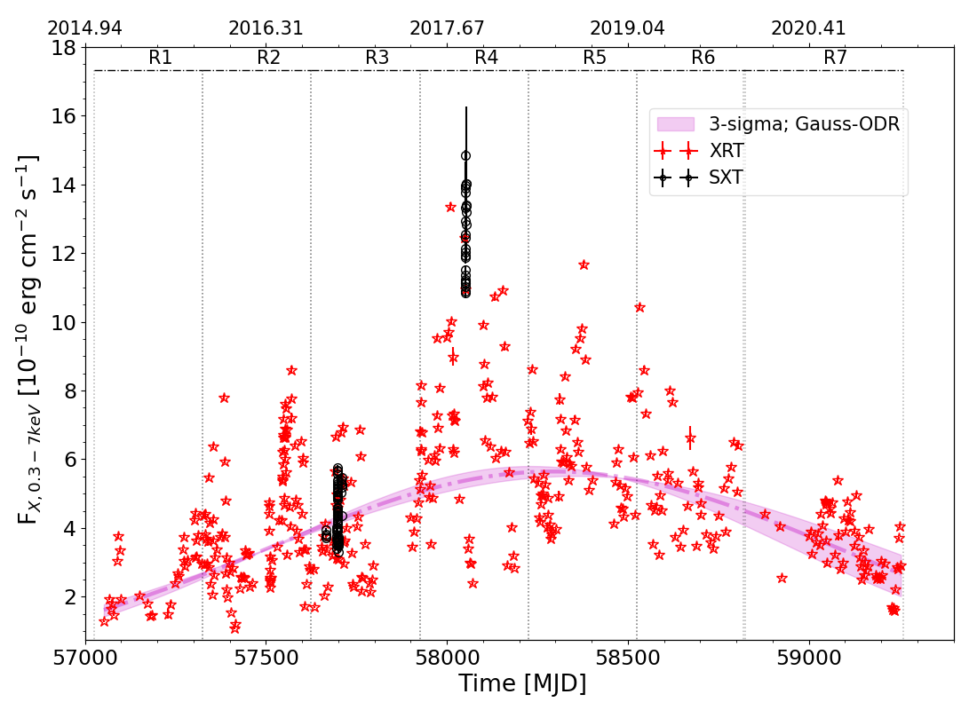
Figure 1: X-ray light curves in the energy range of 0.3-7.0 keV obtained using XRT and SXT data from 2015 December to February 2021. The red stars represent XRT fluxes, whereas the black open circles show SXT fluxes. The shaded region around the best fit dotted curve represents the 3$\sigma$ confidence interval.

3.1 Light Curves and Flux Variations

X-ray light curve in the energy band of 0.3-7.0 keV taken over  6 years (between MJD 57000 to 59260) is shown in Figure 1. The open stars symbolize the integrated fluxes from XRT, whereas the open circles represent the fluxes from SXT. The long SXT exposures are split into several small time intervals of 3500s, within which spectra are extracted and the best fit fluxes are used to construct the light curve (see §2.2.4 for details). However, in order to generate the light curve from XRT, the fluxes are extracted from the best fit model spectra from the individual observations between January 2015 to February 2021.

The overall long-term average flux variation trend which is mathematically characterized by a broad Gaussian peaking at $\sim$ MJD 58233 and FWHM of $\approx$ 785 days. The long-term trend is superimposed by several flares.

The 6 years long XRT lightcurve (Fig.1) is divided into seven segments of 300 days each except the last one which corresponds to 440 days. These segments, R1, R2, R3, R4, R5, R6 and R7, encompass a number of X-ray flares at different epochs sampling the different parts of the above said Gaussian function [See Fig. 1]. The AstroSat observations from 2016 and 2017 fall into R3 and R4, respectively. The following paragraphs summarize the quantitative analysis of the multi-wavelength variability during various X-ray flares around the AstroSat monitoring.

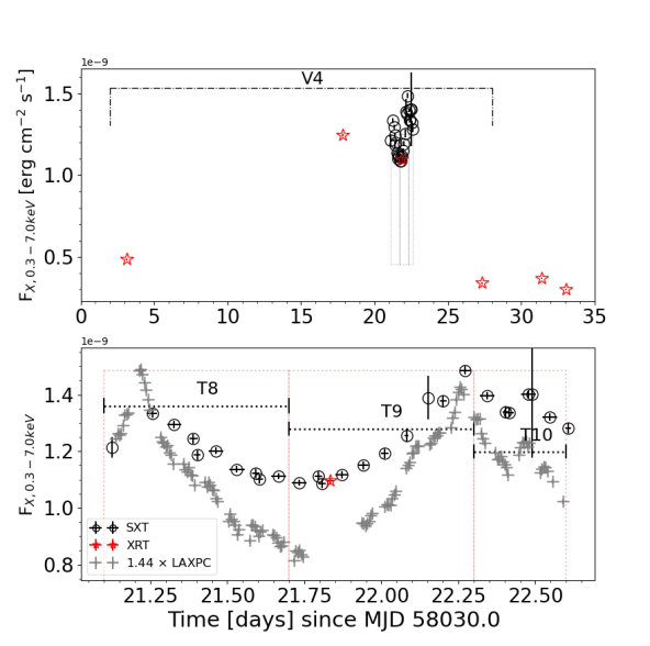
Figure 2: Zoomed-in light curves focusing on the time around the flares observed by AstroSat in 2016 and 2017. Left, hereafter Fig.2a: Various time segments (V1,…,V3) and subgroups (T0,…,T7) during 2016, zooming into the flaring activities in the top and bottom panels. Right, hereafter Fig.2b: Time segment V4 and various subgroups (T8,T9,T10) during 2017, zooming into the bright flaring activities in the bottom panel. The LAXPC light curves are also shown by grey ’+’ markers in the zoomed windows after scaling up to fit in the panels.

The SXT light curves reveal that 1ES 1959+650 exhibits significant flux variations with different time-scales at all the epochs as shown in Figure 2. Therefore, in order to understand the nature of the flux variability during and around the AstroSat observations, four time-segments are created. The basic criteria behind the division of these variability profiles is to distinguish and characterize the X-ray outbursts (doubling/halving time scales & peak flux) which are probably related to the same physical processes which triggered the X-ray activities recorded by the AstroSat. These segments are termed as variability profiles and are denoted by V1, V2, V3 and V4 [See Fig. 2]. Note that the V1, V2 and V3 are subsets of R3, while V4 is a subset of R4. In order to investigate the time dependent spectral behaviour of the flaring activities observed with AstroSat  small portions of V1, V2, V3 and V4 are further subdivided into time-segments denoted by T0, T1,…,T10 [See Fig.2 and Table2 for the details]. These segments zoom-in on to the flux variations during the AstroSat monitoring. Another AstroSat monitoring data with total exposure of $\sim$ 2.9 ks from November 2015, denoted by ‘PV’, is also included in this list to compare the X-ray activities at earlier epochs [See §3.2 for details].

Table 3: Estimation of $\Delta t$ and $F_{var}$

Ttag,prof.	Duration	$\Delta$tD/$\Delta$tH	Fvar,com/Fvar,SXT	FX,p	Ttag,SXT
	[MJD]	[Days]		[erg cm-2 s-1]
				$\times 10^{-10}$
V1	57660.0 - 57670.0	$\uparrow_{XRT}$: 2.69$\pm$0.02	COM.: 0.25$\pm$0.005	4.12
		$\downarrow_{COM.}$: 8.68$\pm$0.05
	57666.22-57666.63	$\uparrow_{SXT}$: 3.09$\pm$0.17	SXT: 0.02 $\pm$0.004		T0
		$\downarrow_{SXT}$: 1.69$\pm$0.01
		$\uparrow_{LAXPC}$: 1.01$\pm$0.008	LAXPC: 0.07$\pm$0.002		T0
		$\downarrow_{LAXPC}$: 0.63$\pm$0.01
V2	57682.6 - 57700.0	–	COM.: 0.19$\pm$0.002
SF1	57682.70–57695.25	$\uparrow_{XRT}$: 8.59$\pm$0.06	SF1: 0.31$\pm$0.006	7.05
		$\downarrow_{XRT}$: 2.31$\pm$0.01
SF2	57696.30-57700.00	$\uparrow_{COM.}$: 2.92$\pm$0.003	SF2: 0.15$\pm$0.003	5.74	T1+T2+(T3/2)
		$\downarrow_{COM.}$: 1.95$\pm$0.01			(T3/2)+T4
	57696.46-57700.00	$\uparrow_{LAXPC}$: 1.49$\pm$0.01	LAXPC: 0.26$\pm$0.001		T1+T2+(T3/2)
		$\downarrow_{LAXPC}$: 0.65$\pm$0.009			(T3/2)+T4
V3	57700.36 - 57714.3	–	COM.: 0.18$\pm$0.004
SF1	57700.36–57709.40	$\uparrow_{XRT}$: 5.93$\pm$0.07	SF1: 0.30$\pm$0.007	6.78
		$\downarrow_{COM.}$: 5.19$\pm$0.08
SF2	57709.40–57713.80	$\uparrow_{COM.}$: 8.89$\pm$0.03	SF2 0.26$\pm$0.009	6.94
		$\downarrow_{XRT}$: 1.10$\pm$0.001
	57708.45-57709.11	$\uparrow_{SXT}$: 1.23$\pm$0.001	SXT: 0.09$\pm$0.003		T7
		–	LAXPC: 0.15$\pm$0.002		T7
		$\uparrow_{LAXPC}$: 0.36$\pm$0.003	LAXPC,SF1: 0.17$\pm$0.003
		$\downarrow_{LAXPC}$: 0.53$\pm$0.005
		$\uparrow_{LAXPC}$: 0.52$\pm$0.004	LAXPC,SF2: 0.12$\pm$0.003
		$\downarrow_{LAXPC}$: 0.18$\pm$0.003
V4	58032.0 - 58058.0	–	COM. : 0.18$\pm$0.002
SF1		$\uparrow_{XRT}$: 10.81$\pm$0.04	SF1: 0.56$\pm$0.005	12.45
		$\downarrow_{XRT}$: 5.06$\pm$0.03
	58051.1-58052.6	–	SXT: 0.09$\pm$0.008		T8+T9+T10
	58051.1 - 58051.7	$\downarrow_{SXT}$: 2.06$\pm$0.03	T8: 0.07$\pm$0.003		T8
SF2	58051.7 - 58052.3	$\uparrow_{SXT}$: 1.14$\pm$0.01	T9: 0.10$\pm$0.009	14.8	T9
	58052.3 - 58052.6	$\downarrow_{SXT}$: 1.60$\pm$0.009	T10: 0.04$\pm$0.004		T10
		–	LAXPC: 0.15$\pm$0.003		T8+T9+T10
		$\downarrow_{LAXPC}$: 0.63$\pm$0.004	T8: 0.17$\pm$0.001		T8
		$\uparrow_{LAXPC}$: 0.54$\pm$0.003	T9: 0.13$\pm$0.001		T9
		$\downarrow_{LAXPC}$: 0.46$\pm$0.003	T10: 0.07$\pm$0.001		T10

Note: T_tag,prof. and T_tag,SXT refer to the tags adopted for defining the variability profiles and time-segments within the SXT light curves, respectively [Ref. Fig.2a, 2b for the details]. SF represents a small flare observed in each segment, where $\uparrow$ and $\downarrow$ represent its doubling ($\Delta t_{D}$) and halving ($\Delta t_{H}$) timescales, estimated for various flares. The subscripts XRT, SXT, LAXPC and COM., refer to the data used from XRT, SXT, LAXPC and combined from the both XRT/SXT, respectively. The F_X,p represents the peak flux in a particular time segment.

The characteristic flux doubling/halving timescales ($\Delta t_{D}$/$\Delta t_{H}$) of the flares in the different variability profiles (V1, V2, V3, V4), using the combined X-ray lightcurve from both SXT & XRT, are derived with $\Delta t=t_{d}\,\times\,ln\,2/|ln(F2/F1)|$ (Saito et al., 2013). Here, $F1$ and $F2$ are the fluxes observed at a time interval of $t_{d}$. The methodology is also applied to the detailed X-ray lightcurve from SXT to obtain the parameters over shorter time-scales [See Table 3 for details]. The variations are further characterised by the fractional variability amplitude ($F_{var}$) defined in Vaughan et al. (2003) and given by

$$F_{var}=\sqrt{\frac{S^{2}-\sigma^{2}_{err}}{x_{m}^{2}}}$$ (1)

$\sigma^{2}_{err}$ is the mean square error of each observations and $S^{2}$ is the sample variance, where $\sigma_{XS}=S^{2}-\sigma^{2}_{err}$ is the excess variance. $x_{m}$ is the unweighted sample mean for N points. The error in $F_{var}$ is given by

$$\sigma_{F_{var}}=\sqrt{\left(\sqrt{\frac{1}{2N}}\,\frac{\sigma^{2}_{err}}{x_{m}^{2}F_{var}}\right)^{2}+\left(\sqrt{\frac{\sigma^{2}_{err}}{N}}\,\frac{1}{x_{m}}\right)^{2}}$$ (2)

The variability time scales ($\Delta$t_D/$\Delta$t_H), $F_{var}$, and peak flux (F_X,p) are derived for the flares in each time-segment (V1, V2, V3, V4) of the long light curves shown in Fig. 2, including both XRT and combined XRT-SXT observations. The values are reported in Table 3.

The multi-wavelength light curves shown in Fig. 3 illustrate the prominent X-ray activities and its counterparts in other energy bands. Some of the X-ray outbursts seem to have associated high energy counterparts in GeV and TeV bands. There have been several communications from the FACT collaboration through ‘Astronomers Telegrams (ATels)’ (Buson et al., 2016; Biland et al., 2016a, b; Biland & FACT Collaboration, 2016a, b) reporting fluxes beyond 1 Crab unit (CU), and 36 private communications to the partners to trigger multi-wavelength observations during moderately high flux states (F_γ $\geq$ 0.5 CU) over the period of 2016-2017. The FACT quick look analysis (QLA) light curve of 1ES 1959+650 shows several flaring episodes. In the following subsections, the detailed variability profiles, the nature of the X-ray flux variations and its multi-wavelength associations are discussed.

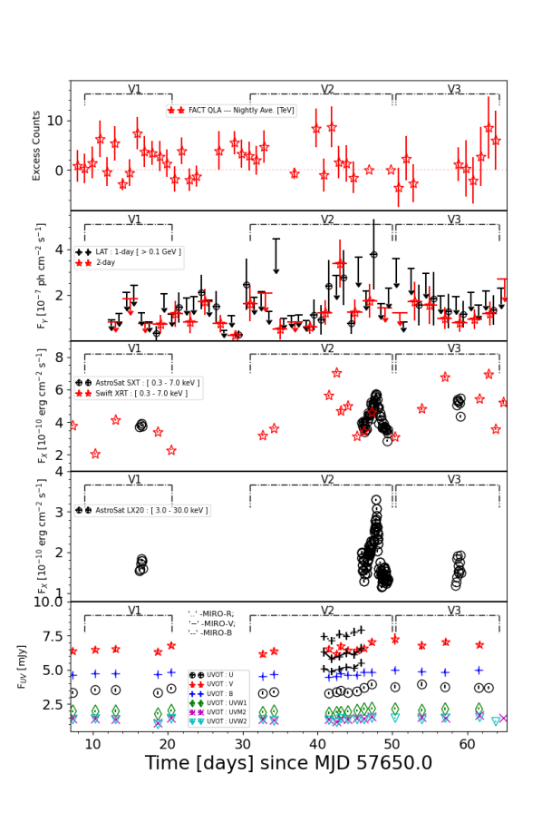
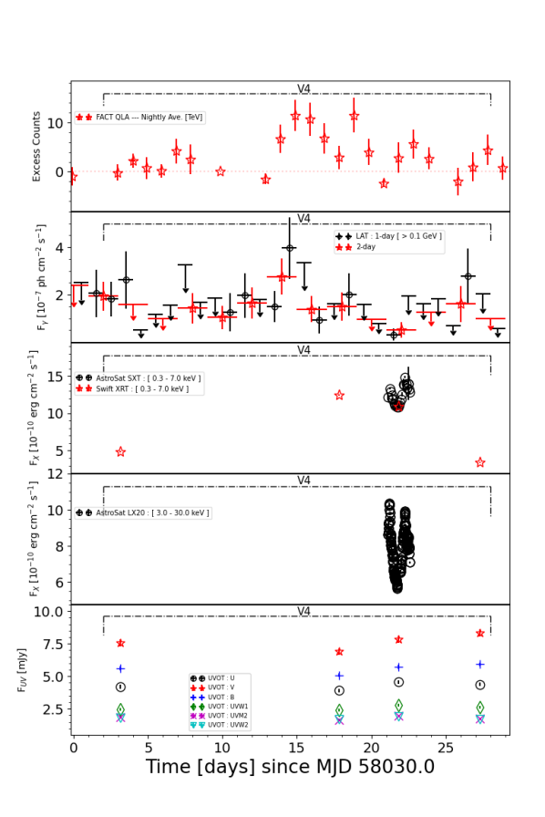
Figure 3: Left: hereafter Fig.3a Multi-wavelength light curves of 1ES 1959+650. From top to bottom: FACT (quick look analysis, binned nightly), Fermi-LAT (binned in 1 day and 2 days), SXT and XRT (binned by orbit), LAXPC and UVOT (U, V, B, UVW1, UVM2 and UVW2 bands) and MIRO (B,V and R bands, binned nightly) during October-November 2016 (corresponds to segments V2 and V3). Right: hereafter Fig.3b Same as left, but for the observations during November 2017 (corresponds to segment V4). Note that 95 % upper limits instead of flux points are used for time-bins where the test statistics (TS) in the LAT light curves are TS$\leq$25.

3.1.1 Variability profile 1 (V1)

The variability profile V1 refers to the light curves around T0 starting from MJD 57660.0 to 57670.0. It also includes four pointings by Swift. The X-ray light curves (see Fig. 2a) show that the observations performed during T0 have been part of a fast varying flux state (F_var $\sim$ 0.25$\pm$0.005) with initial rise ($\Delta$t_D $\sim$ 2.7 days) and fall ($\Delta$t_D $\sim$ 8.7 days). The X-ray light curves in 0.3-7.0 keV (SXT) and 3.0-30.0 keV (LAXPC) bands over T0 show significant flare-like variations (See Table 3 for details). The flux variation in the 3-30.0 keV band is more prominent than in the 0.3-7.0 keV band. As shown in Fig3a, V1 comprises hints of flux variations in the TeV band whereas no variations are observed in the optical/UV and GeV bands.

3.1.2 Variability profile 2 (V2)

V2 corresponds to the light curves during MJD 57682.6 and 57700.0 (see Fig. 2a) which starts 12.5 days after the end of V1. The combined light curves clearly show that V2 encompasses two consecutive X-ray flares with the first one barely covered by XRT (SF1) and the second one entirely observed by the AstroSat (SF2). The peak to peak time difference of the SF1 and SF2 is $\sim$ 6.9 days.

SF1 is highly asymmetric in X-rays, and shows noticeable TeV and GeV activities. SF2, however, while also highly asymmetric in X-rays, hardly shows any variations at other energies. The fastest variations during V2 are observed with LAXPC during SF2 (${\Delta}t_{D}$ = 1.5 days and ${\Delta}t_{H}$=0.65 days). Hence, the X-ray variations during both SF1 and SF2 can be characterized by ‘slow rise and fast decay’ profiles [See Table 3].

The AstroSat light curves are further subdivided into time-segments T1, T2, T3, T4, T5, and T6 [See Fig. 2a]. In addition to the average flux variations over the AstroSat observations, the variability time scales and fractional variability indicate significant variations even during above mentioned T-segments [See Table 3]. Combining the optical/UV fluxes from MIRO and UVOT, we deduce that no significant optical and UV counterparts of the X-ray flares during V2 are seen [Ref. Fig.3a].

3.1.3 Variability profile 3 (V3)

The variability profile V3 extends from MJD 57704.3 - 57714.3, that is, it starts soon after the end of V2. The combined XRT and SXT X-ray light curves during V3 (see Fig. 2a), show that AstroSat pointing T7 is most probably the falling part of an X-ray flare which peaks at the flux (6.78 $\times$ 10^-10 erg cm^-2 s^-1) comparable to the same of V2-SF1. The V3 profile contains two (SF1 and SF2) X-ray flares of nearly similar peak fluxes with the second one decreasing very fast (${\Delta}$t_H = 1.1 day). Both SF1 and SF2 show the ‘slow rise and fast decrease’ already seen in V2. A similar trend is also seen in the LAXPC light curve (3.0-30 keV band), however, the fractional variability is higher than in the SXT band [See Table 3]. There are no obvious counterparts in other energy bands, with the noteworthy exception of a TeV enhancement during SF2.

3.1.4 Variability profile 4 (V4)

The profile V4 extends from MJD 58032.0 to 58058.0 (see Fig. 2b). This time segment signifies the X-ray flux variability around the major activity observed in November 2017.

V4 includes 4 pointings of Swift with one coinciding with the AstroSat observations. The combined X-ray light curve during V4 shows that the X-ray flare observed with AstroSat is part of a prominent MWL activity lasting over $\sim$ 24 days. The Swift light curve alone shows that the source has doubled its flux in merely 15 days from MJD 58033.0 to 58048.0, reaching a record flux of 12.45 $\times$ 10^-10 erg cm^-2 s^-1 in the 0.3-7.0 keV band [Ref. Fig. 2b]. The AstroSat pointing was made 3 days after the XRT peak, that is MJD 58051.0. The AstroSat observations in V4 reveal the highest flux state ever observed (14.8 $\times$ 10^-10 erg cm^-2 s^-1).

The observations with AstroSat lasting $\sim$ 2 days reveal two major sub-flares. The doubling and halving times indicate a slow decline and fast rise in them. Figure 5 and Table LABEL:tab:swtspec_par reveal a significant shift in the synchrotron peak position (E_s,p) over the flare compared to the observations in 2016.

The LAXPC light curve shows a similar behavior as the SXT light curve but exhibits a more pronounced amplitude variability, which is underlined by a higher excess fractional variance ($EV=0.15$) compared to the SXT light curve ($EV=0.08$). As shown in Fig3b, V4 comprises GeV and TeV flares nearly three days prior to the observed X-ray peak. The GeV/TeV fluxes double within $\sim$ 1 day. Interestingly, the GeV flare exhibits a narrower profile than the TeV flare and leads the TeV flare by $\sim$ 1 day. The lack of X-ray data prohibits us to judge whether the GeV/TeV peak corresponds to the (in this case unknown) X-ray maximum or if the X-ray response is delayed. The sub-flare observed with AstroSat, however, corresponds to a low state in the GeV/TeV bands. No significant UV/optical counterparts are seen.

The correlated X-ray activity, along with the shift of the peak position mentioned above, implies that it’s not a simple variation in electron density, but a more complicated spectral change throughout the flare that is responsible for the X-ray flare. This requires time-dependent changes in the magnetic field, the maximum electron Lorentz factor, the Doppler factor of the emission region, or a combination thereof. A more detailed analysis is provided below.

Figure 4: X-ray spectra fitted with a log-parabola model. Top-Left, hereafter 4a: E²F_E v/s E for T0 (black) and T7 (red) extracted from AstroSat observations performed during 05-06 October 2016 and during 16-17 November 2016. Top-Right, hereafter 4b: Same as panel a, but for periods T1, T2, T3, T4, T5, and T6. The various spectra represent different flux and spectral states segmenting different parts of the outburst observed between MJD 57695.9 $-$ 57699.0 (03$-$07, November 2016). Bottom-Left, hereafter 4c: Same as panel a, but for T8, T9 and T10 from the outburst between MJD 58051.1 $-$58052.6, i.e. between 25-26 October 2017. Bottom-Right, hereafter 4d: E²F_E v/s E plots with the respective butterfly diagram representing the best-fit parameters and their uncertainties for all 16 X-ray spectra shown in panels a – d.

3.2 X-Ray Spectral Modeling

The combined X-ray spectra from SXT and LAXPC covering the 0.3-30 keV band from various epochs are fitted to derive the time dependent spectral behavior of the source. For these investigations, the total AstroSat observations are split into 12 segments (see Table 2 and Fig. 2). These time segments are designated as PV, T0, …, T10. The PV segment refers to the $\sim$ 3ks AstroSat pointing of 1ES 1959+650 performed on 20 November 2015. These segments are defined to highlight the changes in the X-ray spectral parameters sampling different parts of the flares and also different average flux states [See Table 2 and Fig. 2 for the definitions of these time-segments].

The combined SXT+LAXPC spectra from the 12 segments are individually modelled with two spectral models (1) TBabs * LogParabola, hereafter M1, and (2) TBabs * Cuttoffpl, hereafter M2. The absorption model component TBabs with the WILM abundance model (Wilms et al., 2000) is used to fit the Galactic neutral hydrogen absorption in the source direction. The LogParabola and CutoffPl models fit a log-parabola and a cut-off power-law shape to the intrinsic spectra, respectively. The input parameter $nH$ is kept fixed to 0.107 $\times$ 10^-22 cm^-2 in both the models M1 and M2 throughout. This value is estimated using 21 cm observations in the source direction (GAL. Coordinate L=98.003370^∘, B=17.669746^∘) using the online tool by the LAB Survey (Kalberla et al., 2005, and relevant reference therein) with the default 0.27^∘ beam. The PV segment does not have a usable LAXPC spectrum and hence, the spectral results correspond to the SXT observations (0.3-7.0 keV) only. The $\chi^{2}$ statistics is used for the spectral modeling throughout.

The best fit parameters from the spectral fitting along with their 2$\sigma$ uncertainties are listed in Table 4. The best fit results show that the observed X-ray spectra can be represented equally well by M1 and M2. We prefer M1 over M2, as (1) it has been used in previous studies, thus allowing for an easy comparison, and (2) the fitting with M2 requires higher systematic uncertainties to be added to the statistical errors to converge the fit. On the other hand, the PV spectrum is fitted with the absorbed powerlaw model (TBabs*powerlaw with fixed nH).

In order to get acceptable $\chi^{2}_{\nu}$ values 4-5% systematic uncertainties are needed in many cases. Normally, 3% systematic uncertainties are recommended for the SXT+LAXPC joint spectral fitting. Panels (a, b, c) in Fig. 4 show the observed spectra for T0 to T10 with the respective best fit models. Fig. 4d presents the model generated spectra in the energy band 0.2$-$12.0 keV. The colored regions around the model spectra are 1$\sigma$ uncertainty intervals for the best fit parameters.

Table 4: The best fit parameters for time-resolved X-ray spectra. The C parameter refers to the relative cross normalization for LAXPC keeping the SXT normalization fixed to 1.

TTag	Log parabola						Exponential Cutoff Power-law
	C	$\alpha$	$\beta$	FX,0.3-8.0keV	Es,p	$\chi^{2}_{\nu}$/dof	$\Gamma$	Ecut	FX,0.3-8.0keV	$\chi^{2}_{\nu}$/dof
				[erg cm-2 s-1]	[keV]				[erg cm-2 s-1]
				$\times$ 10-10					$\times$ 10-10
PV†	-	2.48$\pm$0.04	-	2.09$\pm$0.04	-	1.21/197	2.37$\pm$0.04	13.68	2.02$\pm$0.02	1.31/195
T0	0.85$\pm$0.03	1.98$\pm$0.02	0.36$\pm$0.02	3.17$\pm$0.02	1.07$\pm$0.07	1.6/142	1.97$\pm$0.02	13.68${}^{+1.24}_{-1.06}$	3.26$\pm$0.02	1.80/142
T1	0.85$\pm$0.03	2.07$\pm$0.02	0.33$\pm$0.02	3.20$\pm$0.02	0.78$\pm$0.06	1.08/311	2.11$\pm$0.03	14.75${}^{+1.43}_{-1.21}$	3.16$\pm$0.02	0.91/288
T2	0.84$\pm$0.03	2.03$\pm$0.02	0.36$\pm$0.02	3.57$\pm$0.02	0.91$\pm$0.05	1.29/360	2.06$\pm$0.02	13.28${}^{+0.99}_{-0.87}$	3.69$\pm$0.02	1.21/330
T3	0.83$\pm$0.02	1.99$\pm$0.01	0.38$\pm$0.02	4.42$\pm$0.02	1.03$\pm$0.03	1.78/397	2.04$\pm$0.02	13.07${}^{+0.91}_{-0.80}$	4.57$\pm$0.02	1.09/367
T4	0.89$\pm$0.03	2.09$\pm$0.01	0.40$\pm$0.02	3.14$\pm$ 0.01	0.77$\pm$0.03	1.55/416	2.13$\pm$0.02	11.43${}^{+0.86}_{-0.76}$	3.26$\pm$0.01	1.14/386
T5	0.81$\pm$0.02	2.01$\pm$0.01	0.37$\pm$0.02	4.00$\pm$0.01	0.97$\pm$0.03	1.60/456	2.05$\pm$0.02	13.10${}^{+0.82}_{-0.73}$	4.14$\pm$0.01	1.27/426
T6	0.72$\pm$0.02	2.05$\pm$0.01	0.40$\pm$0.02	3.64$\pm$0.01	0.87$\pm$0.03	1.67/447	2.08$\pm$0.02	11.29${}^{+0.79}_{-0.71}$	3.77$\pm$0.01	1.23/412
T7	1.03$\pm$0.04	1.98$\pm$0.02	0.52$\pm$0.03	3.72$\pm$0.02	1.05$\pm$0.05	1.84/132	1.96$\pm$0.02	9.41${}^{+0.62}_{-0.56}$	3.71$\pm$0.02	1.70/132
T8	0.81$\pm$0.02	1.84$\pm$0.02	0.25$\pm$0.02	10.7$\pm$0.06	2.09$\pm$0.19	1.33/133	1.86$\pm$0.02	25.28${}^{+1.92}_{-1.68}$	10.09$\pm$0.06	1.41/135
T9	0.92$\pm$0.03	1.85$\pm$0.02	0.29$\pm$0.003	10.56$\pm$0.06	1.89$\pm$0.12	1.45/139	1.86$\pm$0.02	19.56${}^{+1.51}_{-1.32}$	10.79$\pm$0.06	1.84/127
T10	0.78$\pm$0.02	1.65$\pm$0.02	0.41$\pm$0.02	12.47$\pm$0.07	2.67$\pm$0.18	1.89/129	1.75$\pm$0.02	14.48${}^{+0.79}_{-0.72}$	12.51$\pm$0.07	1.79/133

Note: The exponential cutoff power-law seems to show low reduced $\chi^{2}$ values in comparison to that from Log Parabola model because of higher systematic (4% instead of 3%). E_s,p values are evaluated from the best-fit Log parabola parameters as described in Appendix A. $\dagger$: The data fits well with powerlaw instead of logparabola model. Also due to poor statistics the cutoff energy is fixed to 13.68 keV as observed during next observations.

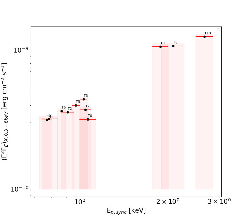
Figure 5: Positions of the synchrotron peaks estimated for the different time bins (T0 …T10) defined in Table 2 and Fig. 2.

Fig. 4 clearly establishes prominent flux and spectral variations. The vertical dashed lines show the positions of the synchrotron peaks (E_s,p) which are calculated using equation A5 and reported in Table 4. The projected synchrotron peak position E_s,p,pv is below 0.2 keV. It also represents the faintest state as observed with AstroSat. The spectra observed in 2016 (T0, …,T7) clearly show significant variations in E_s,p throughout. Fig. 5 illustrates the shift in the synchrotron peaks for various time bins; see also Table 2. Within the 1$\sigma$ confidence intervals (Fig. 5), the shifts in E_s,p are correlated to the flux states for the outbursts in 2016 and 2017.

This investigation establishes that the spectra of 1ES 1959+650 in the 0.3$-$30 keV band become harder with increasing X-ray flux, and subsequently, the peak of the synchrotron emission shifts towards higher energies. The hardening of spectra and shift in E_s,p is linked to the particle energization. These motivate us to investigate the relationship between fluxes and E_s,p further by utilizing a) modelling SXT spectra sampling smaller portions of the flares and, and b) fitting around 400 XRT spectra observed between January 2015 to February 2021. The spectral modelling of the SXT spectra with such a sampling provides us with a unique independent data set representing the two major outbursts in 2016 and 2017, while the integration of the XRT data, sampling the X-ray variations over 6 years, adds to a general understanding of the above relationship. Additional details are discussed in §3.3.

3.3 Correlation Analysis

Table 5: Results from correlation studies:

	$R1=MJD57025.0-57325.0$			$R2=MJD57325.0-57625.0$			$R3=MJD57625.0-57925.0$
	$r_{s}$	$p$		$r_{s}$	$p$		$r_{s}$	$p$
$\alpha$ and $F_{X}$	$-$0.70	1.08$\times 10^{-5}$		$-$0.72	1.45$\times 10^{-17}$		$-$0.69	3.64$\times 10^{-8}$
$E_{s,p}$ and $F_{X}$	0.50	4.0$\times 10^{-3}$		0.79	2.64$\times 10^{-23}$		0.71	9.74$\times 10^{-9}$
$E_{s,p}$ and $\alpha$	$-$0.79	1.26$\times 10^{-7}$		$-$0.85	6.02$\times 10^{-29}$		$-$0.95	1.24$\times 10^{-26}$
$\beta$ and $F_{X,0.3-7\rm\,keV}$	$-$0.11	0.55		$-$0.40	3.37$\times 10^{-5}$		$-$0.25	8.19$\times 10^{-2}$
$\alpha$ and $\beta$	$-$0.10	0.59		0.04	0.69		0.15	0.28
$m$	$-$0.15$\pm$0.03	–		$-$0.06$\pm$0.006	–		$-$0.074$\pm$0.01	–
$b$	2.20$\pm$0.08	–		2.01$\pm$0.03	–		2.19$\pm$0.05	–
Fvar	0.37$\pm$0.009			0.41$\pm$0.001			0.35$\pm$0.002
	$R4=MJD57925.0-58225.0$			$R5=MJD58225.0-58525.0$			$R6=MJD58525.0-58825.0$
	$r_{s}$	$p$		$r_{s}$	$p$		$r_{s}$	$p$
$\alpha$ and $F_{X}$	$-$0.87	1.80$\times 10^{-19}$		$-$0.68	1.75$\times 10^{-9}$		$-$0.37	1.43$\times 10^{-2}$
$E_{s,p}$ and $F_{X}$	0.84	7.55$\times 10^{-17}$		0.74	1.65$\times 10^{-11}$		0.47	1.71$\times 10^{-3}$
$E_{s,p}$ and $\alpha$	$-$0.92	3.26$\times 10^{-24}$		$-$0.98	6.79$\times 10^{-41}$		$-$0.89	4.34$\times 10^{-15}$
$\beta$ and $F_{X,0.3-7\rm\,keV}$	$-$0.13	0.32		$-$0.22	8.64$\times 10^{-2}$		0.02	0.92
$\alpha$ and $\beta$	0.05	0.71		$-$0.21	0.11		$-$0.56	1.27$\times 10^{-4}$
$m$	$-$0.057$\pm$0.005	–		$-$0.05$\pm$0.006	–		$-$0.03$\pm$0.01	–
$b$	2.10$\pm$0.04	–		2.15$\pm$0.04	–		1.98$\pm$0.06	–
Fvar	0.36$\pm$0.002			0.28$\pm$0.001			0.30$\pm$0.002
	$R7=MJD58820.0-59260.0$			$AstroSat$ - Oct., Nov., 2016			$AstroSat$ - Nov., 2017
	$r_{s}$	$p$		$r_{s}$	$p$		$r_{s}$	$p$
$\alpha$ and $F_{X}$	$-$0.63	4.13$\times 10^{-8}$		$-$0.44	7.66$\times 10^{-5}$		$-$0.81	4.07$\times 10^{-7}$
$E_{s,p}$ and $F_{X}$	0.69	3.71$\times 10^{-10}$		0.52	2.04$\times 10^{-6}$		0.83	7.75$\times 10^{-8}$
$E_{s,p}$ and $\alpha$	$-$0.90	1.09$\times 10^{-23}$		$-$0.77	6.79$\times 10^{-16}$		$-$0.68	9.71$\times 10^{-5}$
$\beta$ and $F_{X,0.3-7\rm\,keV}$	0.068	0.59		$-$0.089	0.44		$-$0.11	0.58
$\alpha$ and $\beta$	$-$0.48	7.41$\times 10^{-5}$		$-$0.47	1.88$\times 10^{-5}$		$-$0.23	0.25
$m$	$-$0.09$\pm$0.01	–		$-$0.04$\pm$0.009	–		$-$0.05$\pm$0.004	–
$b$	2.13$\pm$0.05	–		2.01$\pm$0.04	–		2.23$\pm$0.05	–
Fvar	0.26$\pm$0.002			0.24$\pm$0.003			0.087$\pm$0.007

Note: Here, $r_{s}$ is the Spearman rank co-efficient and $p$ denotes its null hypothesis probability. $m$ and $b$ are respectively, the slope and the intercept of the best-fit EMCEE straight line between $\alpha$ v/s $F_{X,0.3-7\rm\,keV}$. F_var is the fractional variability amplitude.

This section describes the detailed correlation analysis between various spectral parameters and other dependent quantities for the time-segments R1,…,R7 and two sets of AstroSat observations [Fig. 1], separately. The $\alpha$ v/s F_X,0.3-7keV distribution is fitted with a straight-line and is depicted in the Fig.6a. The various pairs of colors and symbols represent the different R segments. The lines are modelled with slope (m) and intercept (b) as free parameters. In order to extract the best fit parameters, the least square regression (LS), maximum likelihood minimization (ML) and Monte Carlo Markov Chain (MCMC) techniques are used. For the MCMC calculations, the EMCEE tool in python (Foreman-Mackey et al., 2013), which is an MIT licensed pure-Python implementation of the Goodman & Weare (2010) Affine Invariant MCMC Ensemble sampler, is used. The best fit parameters derived from the LS and ML techniques are used as initial parameters for the MCMC technique. The thin colored lines in Fig. 6 represent sample lines obtained with the MCMC method, whereas thick dashed lines correspond to the best fits derived with the MCMC technique.

The total of 81 time-resolved spectra extracted from SXT, as described in §2.2.4, are grouped into two parts. The first part covers the three epochs in 2016 and the second for the observations in 2017. These data sets are also modeled using the same methods as described above. The correlations between best fit spectral parameters ($\alpha$ and $\beta$) v/s X-ray flux (F_X,0.3-7keV), E_s,p v/s F_X,0.3-7keV, and $\alpha$ and $\beta$ are explored for all the R segments. The readers are referred to Table 5 for the details of the correlation indicators of various pairs from different R segments and respective best fit parameters of the line.

The index $\alpha$ shows strong correlations with the integrated flux in the 0.3-7.0 keV band for all data segments. It is clear from this figure that most of the time the X-ray spectrum of 1ES 1959+650 gets harder with increasing flux. However, the slopes of the index v/s $F_{0.3-7.0keV}$ relationships for the different time segments differ quite a lot. Especially, the slopes (m) for R1 and R7 are higher than for the other segments. Interestingly, R1 and R7 sample the increasing and decreasing tails of the Gaussian fit of the long-term X-ray light curve, respectively.

The ($m$, $b$) pairs, where $m$ and $b$ are slope and intercept for the fit on the $\alpha$–F_X,0.3-7keV plane, for the AstroSat observations in 2016 and R3, differ significantly. Whereas, the slope of AstroSat observations in 2017 matches the one in R4, though both showing different intercepts. Note that the AstroSat observations mainly sample spectra around particular outbursts, while the Swift observations are spread over a longer duration and hence represent a general behaviour over long periods.

The right panel of Fig. 6b shows the flux dependence of the index (top) and the curvature parameter (bottom). The best fit lines for the R segments are not plotted in the top panel for the sake of clarity. The two sets of AstroSat observations clearly represent two spectrally distinct states of variability of 1ES 1959+650. As clearly shown in Fig. 6, the outburst in 2017 does not only exhibit the highest X-ray flux, but also follows an entirely different track in the spectral-index – flux plane.

Fig. 7 visualizes the confidence intervals and probability distribution for the best fit parameters corresponding to the AstroSat observations in 2016 and R3, respectively. The plots are made using the python package corner, which corresponds to the MCMC fitting method. These diagnostic plots are indicative of a reasonably good convergence and an acceptable quality of the parameter estimations. The correlations between flux enhancements and changes in the spectral parameters $\alpha$ and $\beta$ may provide unique information about the energization of particles responsible for the flux enhancements during a particular flare. Studies by other authors (MAGIC Collaboration et al., 2020; Kapanadze et al., 2018b, a; Krawczynski et al., 2004a) have shown that for a handful of blazars the curvature and index are inversely correlated with an increase in flux. More specifically, an increase in flux is accompanied by a hardening of the spectrum (decreasing $\alpha$) and a decrease in curvature (decreasing $\beta$). The spectral constraints derived for the AstroSat-SXT and Swift-XRT observations confirm the strong positive correlations between the flux and the hardening of the spectrum. However, owing to the large uncertainties, the curvature parameter $\beta$ (shown in the bottom panel of Fig. 6b) does not show a significant correlation with the flux.

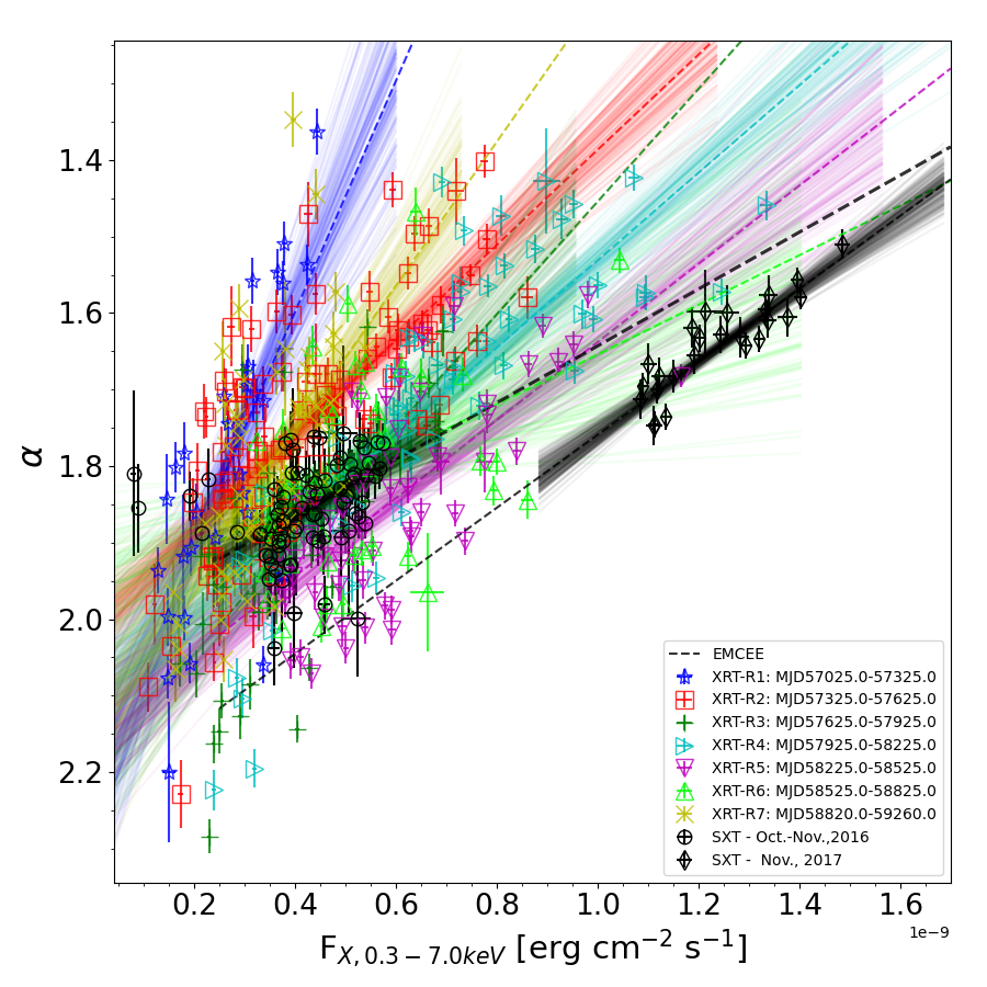
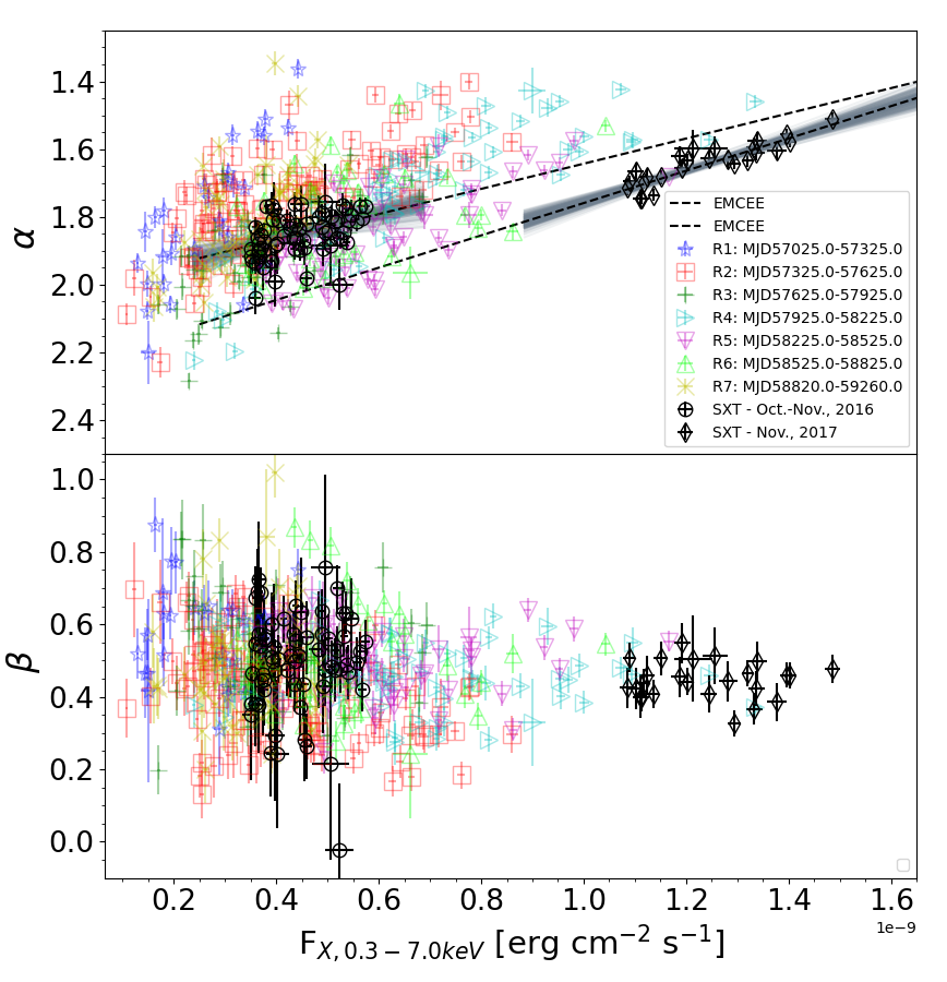
Figure 6: Left, hereafter Fig. 6a: Spectral slope $\alpha$ vs. integrated X-ray flux in the 0.3-7.0 keV band extracted from the time-resolved spectral modeling of SXT observations and the spectra from individual XRT observations starting from 2015-01-04 to 2021-02-15. The open black circles and open black diamonds refer to the SXT observations in 2016 and 2017, respectively. The other XRT observations are divided into seven time segments(R1,…,R7) and are shown by various symbols and colors as described in the legends. The dashed lines of different colors show the best fit linear regressions using the EMCEE method. The various colored thin solid lines indicate the spread around the best fit lines for a particular group of data. Right, hereafter Fig. 6b: Best fit linear correlations with data on $\alpha$ (top panel) and $\beta$ (without any fit — bottom panel) vs. flux. For clarity, the top panel does not include best fit lines for the various time-groups of XRT observations to illustrate the offset between the spectral-index dependencies on flux between the flares in 2016 and 2017.

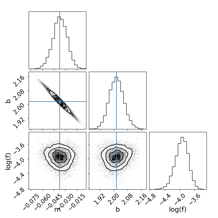
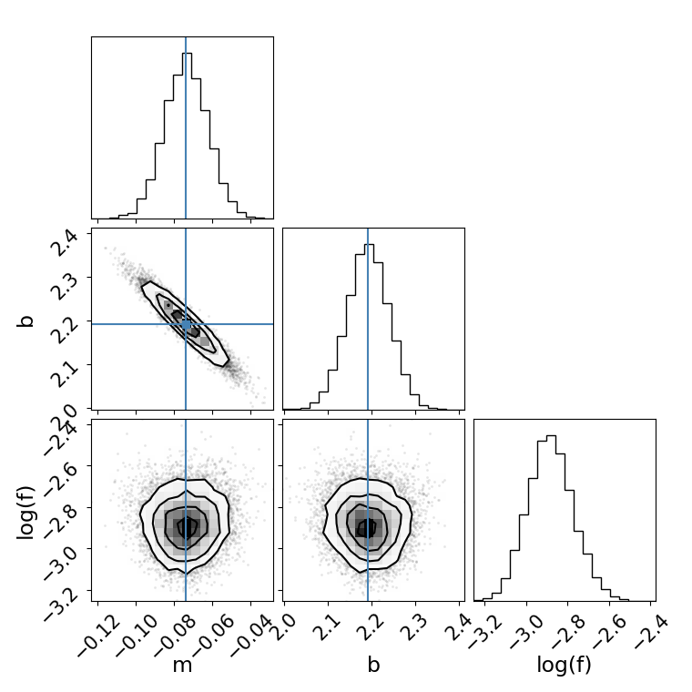
Figure 7: Diagnostics plots for the best fit parameters for the $\alpha$ v/s flux correlations. Left, hereafter Fig. 7a: Plot for the time-resolved SXT spectra from the 2016 flare. Right, hereafter Fig. 7b: Plot for all the XRT spectra observed by Swift over the period MJD 57026 to MJD 57637.

These spectral changes result in a shift of the peak position of the X-ray part of the SED and hence in the position of the synchrotron peak. Such a shift of the synchrotron peak towards higher energies with increasing integrated flux is seen in most HBLs and is equivalent to the “bluer-when-brighter” trend seen in the optical continuum spectra of many BL Lac objects (Böttcher et al., 2010; Dai et al., 2011; Bhatta et al., 2018; Kaur et al., 2017). The best fit $\alpha$ and $\beta$ values are used in equation A5 to derive the position of the peak of the synchrotron component.

Fig. 8a shows the relationship between the synchtrotron peak energy (E_s,p) and the spectral parameters $\alpha$ and $\beta$, respectively. The index parameter $\alpha$ is well correlated with the synchrotron peak position above an energy of $\sim 0.5$ keV, while such a statement cannot be made for the curvature parameter $\beta$.

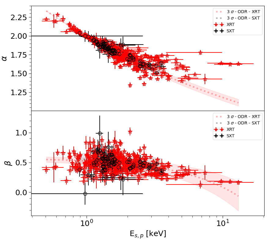
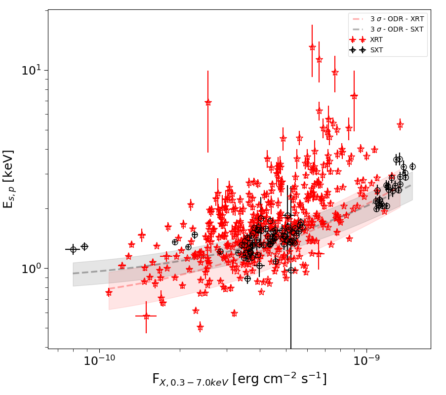
Figure 8: Synchrotron Peak Position and Unabsorbed X-ray flux. Top, hereafter Fig. 8a: Dependence of the spectral slope ($\alpha$; top panel) and the curvature ($\beta$; bottom panel) on the position of the synchrotron peak (E_s,p). The filled red stars represent the XRT data whereas the measurements from the SXT are shown by filled black circles. Bottom, hereafter Fig. 8b: Correlations between the estimated synchrotron peak positions and the integrated X-ray flux measured in the 0.3-7.0 keV band.The dotted red and black lines represent the best fit linear correlations for XRT and SXT observations, respectively. The shaded areas around the best fit curves in both the figures represents 3$\sigma$ confidence interval.

Fig. 8b shows the relationship between E_s,p and the integrated flux F_X,0.3-7.0keV, confirming the trend of the synchrotron peak shifting to higher energies with increasing flux. While the relationship between E_s,p v/s $\alpha$ is well represented by a power-law function, the relationship between F_X,0.3-7.0keV and E_s,p is reasonably fitted with a linear function (All XRT: slope=1.47$\pm$0.11, intercept=0.63$\pm$0.04; All SXT:slope=1.21$\pm$0.07, intercept=0.84$\pm$0.05). In order to further test the correlations, we have performed a Spearman rank correlation analysis of these observable parameters for the spectra obtained during R1,…,R6, and the results are reported in Table 5.

3.4 SEDs, Modeling and Interpretation

The X-ray light curves shown in Fig. 3 indicate the presence of clearly discernible, individual flares, both in 2016 and 2017. We interpret these events as the result of mildly relativistic shocks propagating through the jet of 1ES 1959+650. In order to model the light curves and SEDs during the period of our AstroSat observations in 2016 and 2017, we employ the time-dependent shock-in-jet model of Böttcher & Baring (2019). In this model, hybrid thermal + non-thermal electron distributions are generated via a Monte-Carlo simulations (Summerlin & Baring, 2012) of diffusive shock acceleration by a mildly relativistic, oblique shock. As a representative choice of shock parameters, we assume a shock speed of $v_{s}=0.71$ c (in the co-moving frame of the jet material), a magnetic-field obliquity of $\Theta_{\rm Bf1}=32^{o}.3$, an up-stream gas temperature of $5.45\times 10^{7}$ K, and a compression ratio of $r=3.71$ (see Böttcher & Baring, 2019, for a motivation and discussion of these choices). The Monte-Carlo simulations of diffusive shock acceleration parameterize the electrons’ mean free path to pitch-angle scattering as $\lambda_{\rm pas}=\eta_{0}\,r_{g}\,p^{\alpha-1}$ where $r_{g}$ is an electron’s Larmor radius and $p$ its momentum. $\eta_{0}$ and $\alpha$ are free parameters in the simulation. Since $r_{g}\propto p$, the mean free path scales as $\lambda_{\rm pas}\propto p^{\alpha}$.

The time-dependent radiative output from the resulting hybrid electron distributions is evaluated using the radiation transfer schemes of Böttcher & Chiang (2002); Böttcher et al. (2013b). In addition to $\eta_{0}$ and $\alpha$, free parameters of the model are the shock-dissipated power transferred to relativistic electrons (termed “injection luminosity”, $L_{\rm inj}$, in the following), the magnetic-field strength $B$, the bulk Lorentz factor $\Gamma$ of the emission region’s propagation along the jet, the viewing angle $\theta_{\rm obs}$, and the radius $R$ of the emission region, which is assumed spherical for the purpose of the radiation-transfer simulations. $L_{\rm inj}$, $B$, and $R$ are defined in the co-moving frame of the emission region, while $\theta_{\rm obs}$ is the viewing angle in the observer’s frame.

Since we find a satisfactory fit to snap-shot SEDs and light curves of 1ES 1959+650 with synchrotron and synchrotron-self-Compton (SSC) as the dominant radiation mechanisms (i.e., a pure leptonic SSC model), we do not consider any contribution from putative external radiation fields to the target photon field for Compton scattering to produce the $\gamma$-ray emission.

Our fitting procedure starts out with a quiescent-state configuration, reproducing the low-state SED of 1E 1959+650, shown by the black model curves in Figs. 9a and 10a, with model parameters listed in Tab. 6.

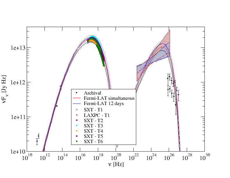
Figure 9: Model fits to SEDs and light curves of 1ES 1959+650 during the AstroSat observations in 2016. Top left (a): Snap-shot SEDs at various times during the simulation; top right (b): Model fits to the AstroSat light curves; bottom left (c): Predicted hardness-intensity correlations in various energy bands. Note that for plotting on the same scale, the 100 keV curve has been shifted up in flux (i.e., right) by a factor of 10, while the 1 GeV curve has been shifted up in spectral index (i.e., down in the plot) by 1; bottom right (d): Predicted discrete correlation functions between light curves in various energy bands.

Table 6: Parameters of our model fits to the quiescent-state SEDs of 1ES 1959+650 in 2016 and 2017, respectively.

Parameter [units]	2016	2017
$\eta_{0}$	60	40
$\alpha$	1.9	1.8
$L_{\rm inj}$ [erg/s]	$2.5\times 10^{40}$	$2.8\times 10^{40}$
$B$ [G]	0.15	0.08
$\Gamma$	20	20
$\theta_{\rm obs}$ [deg]	2.87	2.34
$R$ [cm]	6.e15	1.e16

The zoomed-in light curves in Figs. 9b and 10b clearly suggest that the observed X-ray flaring behaviours both in 2016 and 2017 cannot be modelled by one single, impulsive particle acceleration event, but they are indicative of a succession of several shocks throughout the emission region. Specifically, in order to find a satisfactory representation of both the SXT and the LAXPC light curves during 2016, a succession of 4 shocks of different strength is required. All shocks are characterized by an increased injection luminosity and a global decrease of the pitch-angle mean free path, parameterized by a slightly smaller value of $\eta_{0}$. A consequence of this change is more efficient particle acceleration to higher energies, resulting in the observed larger variability amplitude in the LAXPC (3 – 30 keV) band compared to the SXT (0.3 – 7 keV) band. The parameters adopted for the 4 shocks in our 2016 simulation are listed in Table 7. Representative snap-shot SEDs are shown in Fig. 9a, and the LAXPC and SXT light curves and model fits are presented in Fig. 9b. Since both the UV and Fermi-LAT $\gamma$-ray light curves consist of only very few points (and upper limits), they are not constraining for our fits and are not shown in the figure. We have, however, verified that our model predictions are consistent with the data. Figs. 9c and 9d show the predicted spectral hysteresis in a hardness-intensity diagram at various photon energies, and the predicted cross-correlations between the light curves at different photon energies, respectively.

Table 7: Parameter variations for the fits to MWL light curves and SEDs in 2016.

Parameter [units]	$L_{\rm inj}$ [erg/s]	$\eta_{0}$	$\alpha$
Quiescence	$2.5\times 10^{40}$	60	1.9
Shock 1	$3.0\times 10^{40}$	50	1.9
Shock 2	$3.5\times 10^{40}$	50	1.9
Shock 3	$4.1\times 10^{40}$	40	1.9
Shock 4	$3.4\times 10^{40}$	50	1.9

The observed hardness-intensity correlations plotted in Fig. 6 (left) indicate a systematic offset by a factor of $\sim 2$ in flux of the data from 2017 with respect to the 2016 data in flux. However, within the individual yearly data sets, they show consistent harder-when-brighter trends. Such a systematic offset may be explained by a slight change of the Doppler factor (by a factor of $\sim 1.2$) without any changes in the underlying particle-acceleration and emission physics. A slight change of the viewing angle (from $\theta_{\rm obs}=2.^{o}87$ in 2016 to $2.^{o}34$ in 2017) is sufficient to reproduce such a change in Doppler factor (from 20 to 24). This forms the basis of our modeling of SEDs and X-ray light curves in 2017. Only slight modification of other model parameters are required for our quiescent-state fit to the 2017 SEDs (see Tab. 6).

Figure 10: Same as Fig. 9, but for the AstroSat observations in 2017. Note that in the panel c (bottom left), the 1 GeV hardness-intensity curve has been shifted up (i.e., right) in flux by a factor of 10 and up in spectral index by 1 (i.e., down in the plot) for plotting on the same scale as the other curves.

The X-ray light curves (Fig. 10b) from the 2017 AstroSat observations show two clearly distinct major flaring episodes near the beginning and the end of the observations. Clearly, again, multiple shocks are required in order to provide a satisfactory representation of these complex light curves. Specifically, we find a good match with the SXT and LAXPC adopting a succession of 5 shocks, all characterized by a larger injection luminosity compared to the quiescent state as well as more efficient particle acceleration to higher energies. The latter is primarily achieved through a change in the mean-free-path parameter $\eta_{0}$. The parameters adopted for the 5 subsequent shocks are listed in Tab. 8.

Table 8: Parameter variations for the fits to MWL light curves and SEDs in 2017.

Parameter [units]	$L_{\rm inj}$ [erg/s]	$\eta_{0}$	$\alpha$
Quiescence	$2.8\times 10^{40}$	40	1.8
Shock 1	$3.5\times 10^{40}$	30	1.7
Shock 2	$3.0\times 10^{40}$	30	1.8
Shock 3	$3.6\times 10^{40}$	25	1.8
Shock 4	$4.3\times 10^{40}$	25	1.8
Shock 5	$5.1\times 10^{40}$	15	1.8

Given the relative simplicity of our model setup and the complexity of the SXT and LAXPC light curves both in 2016 and 2017, the correspondence between the observed X-ray light curves and our model predictions is remarkable. For both years, we reproduce the observed general harder-when-brighter trend (see Fig. 6) with only very moderate spectral hysteresis, which is smaller than the error bars on the SXT and LAXPC flux and spectral-index points, especially for 2016. The model 1 keV vs. 10 keV time lags may be considered as a proxy to the observed trends between SXT and LAXPC. For 2016, our model predicts a lag of $\sim 1$ hr of the SXT (1 keV) light curve behind the LAXPC (10 keV) one, while for 2017, this lag is predicted to be slightly larger, at $\sim 1.5$ hr. Predicted lags between X-ray and $\gamma$-ray bands are equally of the order of $\lesssim 1$ hr.

4 Discussion and Summary

Our analysis, presented above, clearly establishes that 1ES 1959+650 underwent significant flaring activity in X-rays over the 6 years during 2015 to 2021 (see Fig. 1). The overall long-term X-ray variability over these years shows a profile that is symmetric and well represented by a broad (FWHM$\sim$785 days) Gaussian function peaking around April 2018. Such a long-term symmetric flux variation is suggestive of a change in the viewing angle, and hence in the Doppler boosting, as the main driver. Most probably the inner jet is curved. Unfortunately, the data coverage is not sufficient to test the jet-precession theory, which predicts periodic changes in the flux. The X-ray light curves show that there are many short-time-scale variations superimposed on the long-term symmetric variations throughout (Fig. 2).

The detailed light curves observed with AstroSat cover different prominent X-ray flares and exhibit shorter-time-scale variations (see Table 3 for time-scales and the variability amplitudes.) During the X-ray outburst in 2016 the source also exhibits noticeable activity at $\gamma$-ray energies, even though no clear correlation pattern emerges. Most importantly, V2-SF1 is accompanied by simultaneous GeV/TeV activity, whereas V2-SF2 (total span of $\sim$ 2 days) seems to be a pure orphan X-ray flare.

In 2017 1ES 1959+650 underwent several prominent X-ray outbursts including the one observed with AstroSat, which seems to have a twin-flare-like profile within $\sim$ 2 days (see Fig. 2b). During this period, 1ES 1959+650 broke its historical X-ray flux record (in the 0.3$-$7.0 keV band) reaching a new maximum, which has not been exceeded until the time of writing (see Fig. 1). The observed X-ray flux showed two high-amplitude, short-time-scale flares without any counterpart at other wavelengths. Therefore, the variations observed with AstroSat are again orphan. Interestingly, a few days prior to the X-ray observations prominent variability took place at $\gamma$-ray energies. Unfortunately, the lack of multiwavelength observations during that time precludes any correlation analyses.

The AstroSat observations of the X-ray activity periods in 2016 and 2017 are unique as these provide such a detailed variability profiles for 1ES 1959+650 for the first time. The light curves in the 0.3-7.0 keV band are highly correlated with the ones in the 3.0-30 keV band for all the epochs in 2016 and 2017.

However, during all epochs, the variability amplitude is larger in the hard X-ray band compared to the soft X-rays. The shortest variability time-scale ($\Delta$t; here characterized by the doubling or halving time scales) may be used to calculate an upper limit on the size of the emission region using the light-travel-time argument, R $\leq$ $\frac{c\delta{\Delta}t}{(1+z)}$. The smallest inferred limit on the size of the emission region for the activity periods in 2016 and 2017 are 2.9 mpc and 7.4 mpc, respectively.

The X-ray spectral investigations reveal significant changes in the spectral shapes for different flares and also for the different segments of the AstroSat observations (T0, T1,…,T10). The spectral changes follow a harder-when-brighter trend as is typical for many blazars. The broad-band X-ray spectra (0.3-30 keV) are best represented by a log-parabola model. A similar investigation using time-resolved spectra from SXT and long-term observations from XRT provide similar trends. However, different sets of flares (R1,…,R7) show a slightly different relation between flux and spectral index: Different R’s populate significantly different tracks in the $\alpha$ -F_X,0.3-7keV plane. The R-segments representing the the beginning (R1) and end (R7) of our data set, on the other hand, show extreme slopes (See Table 3 for details).

The time-resolved spectroscopy of the AstroSat observations reveals a strong correlation between the slope ($\alpha$) and the flux (F_X,0.3-7.0keV) for both observation periods in 2016 and 2017, similar to the enveloping R-segments (R3 and R4, respectively). However, the tracks in the $\alpha$ v/s F_X,0.3-7.0keV plane of the AstroSat data sets are significantly different from the corresponding R-segments. The best fit lines of $\alpha$ v/s F_X,0.3-7.0keV for the two sets comprise significantly different tracks indicating that the spectrum exhibits stronger hardening with increasing flux in 2017 compared to 2016 (see Table 3). This indicates that the ”bluer-when-brighter” trend was stronger in 2017 than in 2016, which is also supported by the strong, positive correlation of the synchrotron peak energy ($E_{s,p}$) with the X-ray flux.

The various X-ray SEDs, namely T1 to T6 from the flare in 2016 and T8 to T10 from the flare in 2017, are combined to generate two broad-band SEDs. A model based on diffusive shock acceleration by mildly relativistic shocks in the jet of 1ES 1959+650 is able to simultaneously reproduce those snap-shot SEDs and the AstroSat light curves of both flaring episodes in 2016 and 2017. In this model, multi-wavelength flares are caused by shock-generated turbulence, leading to a reduction of the electrons’ mean free path to pitch-angle scattering ($\lambda_{\rm pas}$) and, thus, more efficient particle acceleration. The instantaneous interplay between shock acceleration and self-consistent radiative (synchrotron, SSC, and external Compton) cooling of the particles in the emission region results in characteristic flux and spectral variability patterns, consistent with the observed ones. The different flux states between the two flares are well reproduced by a change in the Doppler factor, mediated by a slight change of the viewing angle ($\Delta\theta$ $\sim$ 0.5^∘) within $\sim$ 1 year, and a reduction of the magnetic field.

This manuscript highlights the flux evolution of various X-ray flares observed between December 2015 and February 2021, their spectral properties, and their correlations. Additionally, a time-dependent leptonic model indicates the particle acceleration responsible for the two X-ray flares in 2016 and 2017 covered in detail with AstroSat. This work additionally avails a huge dataset to the community with the spectral parameters spanning 6 years of X-ray monitoring of 1ES 1959+650. While a detailed study of the spectral parameters of the $\gamma$-ray bands, as well as their correlation with the X-ray bands, is not possible with the currently available data, such a study may shed light on the emission mechanisms during flaring activities. The future MeV/GeV/TeV facilities like AMIGO and CTA, shall provide key data for the such investigations.

Appendix A Appendix - I; Synchrotron Peak Frequency

The functional form of the mathematical model used to fit the X-ray spectra of 1ES 1959+650 is given by :

$$\frac{dN}{dE}=N_{0}\left(\frac{E}{E_{0}}\right)^{-\left[\alpha+\beta\times\log_{10}\left(\frac{E}{E_{0}}\right)\right]}$$ (A1)

where E₀ is known as pivot energy, $\alpha$ is the photon index and $\beta$ is the curvature parameter of the model. The equivalent equation valid for fitting the $\nu$F_ν plot i.e. X-ray part of the SEDs

$$\nu F_{\nu}=N_{0}\left(\frac{\nu}{\nu_{0}}\right)^{\left[2-\alpha-\beta\times\log_{10}\left(\frac{\nu}{\nu_{0}}\right)\right]}$$ (A2)

It is well established that in most of the flux states the synchrotron peak of the broad-band SED of 1ES 1959+650lies between 0.3 to 10.0 keV. Hence it is most likely that the maxima of equation A2 refers to the synchrotron peak energy. That is, $\nu_{syn,peak}$ or $\nu_{s,p}$ [E_s,p] corresponds to the solution of equation $\frac{d(\nu F_{\nu})}{d\nu}$ = 0

$$\frac{d(\nu F_{\nu})}{d\nu}=N_{0}(2-\alpha)\left(\frac{\nu}{\nu_{0}}\right)^{(1-\alpha)}\left(\frac{\nu}{\nu_{0}}\right)^{-\beta\times\log_{10}(\frac{\nu}{\nu_{0}})}-N_{0}\left(\frac{\nu}{\nu_{0}}\right)^{(2-\alpha)}\times\left(\frac{2\beta\times\log_{10}\left(\frac{\nu}{\nu_{0}}\right)}{\nu}\right)\times\left(\frac{\nu}{\nu_{0}}\right)^{-\beta\times\log_{10}(\frac{\nu}{\nu_{0}})}$$ (A3)

i.e.,

$$\frac{d(\nu F_{\nu})}{d\nu}=N_{0}\left[(2-\alpha)-2\beta\times\log_{10}\left(\frac{\nu}{\nu_{0}}\right)\right]\times\left(\frac{\nu}{\nu_{0}}\right)^{[1-\alpha-\beta\times\log_{10}\left(\frac{\nu}{\nu_{0}}\right)]}$$ (A4)

This means $\frac{d(\nu F_{\nu})}{d\nu}$ = 0 $=>$

$$\nu_{s,p}=\nu_{0}\times 10^{(\frac{2-\alpha}{2\beta})}\,\,\,or;\,\,\,E_{s,p}=E_{0}\times 10^{(\frac{2-\alpha}{2\beta})}$$ (A5)

here, $\nu_{0}$ corresponds to the frequency of the photons at 1 keV i.e., $\nu_{0}$ = 2.4180 $\times$ 10¹⁷ Hz. Therefore, for a given index $\alpha$ and curvature $\beta$ we can estimate the position of the synchrotron peak using equation A5. The same formalism is derived as equation 3 in Massaro et al. (2004).

Table 9: AstroSat  data and the best fit parameter corresponding the model : M1. The complete table is available in a machine-readable format in the published journal or via email on request.

ObsID	Time	Exp.	$\alpha$	$\beta$	$\chi^{2}_{\nu}$/dof	FX,0.3-7keV	Es,p
						$\times$ 10-10
	[MJD]	[s]				[erg cm-2 s-1]	[keV]
A02_199T01_9000000708	57666.25	2886.3	1.85$\pm$0.02	0.45$\pm$0.06	267.3/230	3.71$\pm$0.06	1.46$\pm$0.12
A02_199T01_9000000708	57666.39	4041.7	1.77$\pm$0.02	0.56$\pm$0.05	348.9/267	3.81$\pm$0.05	1.61$\pm$0.1
A02_199T01_9000000708	57666.52	2938.6	1.81$\pm$0.02	0.5$\pm$0.06	228.5/238	3.94$\pm$0.06	1.56$\pm$0.12
A02_199T01_9000000708	57666.6	3430.7	1.84$\pm$0.02	0.45$\pm$0.05	280.9/248	3.76$\pm$0.05	1.51$\pm$0.12
G06_086T01_9000000774	57695.9	380.4	1.99$\pm$0.07	0.29$\pm$0.18	46.9/53	3.98$\pm$0.19	1.03$\pm$0.29
G06_086T01_9000000774	57695.93	1286.2	1.89$\pm$0.04	0.47$\pm$0.08	146.2/159	3.97$\pm$0.08	1.32$\pm$0.13
G06_086T01_9000000774	57696.0	924.8	1.87$\pm$0.04	0.56$\pm$0.1	112.1/114	3.77$\pm$0.1	1.3$\pm$0.13
G06_086T01_9000000774	57696.07	577.7	1.9$\pm$0.06	0.38$\pm$0.14	75.1/74	3.66$\pm$0.13	1.34$\pm$0.28
G06_086T01_9000000774	57696.13	233.0	1.88$\pm$0.09	0.24$\pm$0.21	33.4/33	4.02$\pm$0.22	1.78$\pm$1.17
G06_086T01_9000000774	57696.19	706.1	1.93$\pm$0.05	0.25$\pm$0.12	94.5/86	3.89$\pm$0.12	1.39$\pm$0.39
G06_086T01_9000000774	57696.26	370.9	1.78$\pm$0.08	0.54$\pm$0.18	47.1/53	3.95$\pm$0.17	1.61$\pm$0.38

Table 10: Swift  data and the best fit parameter corresponding the model : M1. The complete table is available in a machine-readable format in the published journal or via email on request.

ObsID	Time	Exp.	$\alpha$	$\beta$	$\chi^{2}_{\nu}$/dof	FX,0.3-7keV	Es,p
						$\times$ 10-10
	[MJD]	[s]				[erg cm-2 s-1]	[keV]
00035025010	53884.16	3280.4	2.01$\pm$0.01	0.49$\pm$0.03	336.6/307	3.26$\pm$0.02	0.97$\pm$0.03
00035025118	56856.74	1276.3	1.83$\pm$0.04	0.72$\pm$0.09	105.1/115	1.32$\pm$0.03	1.32$\pm$0.09
00035025132	57052.09	1881.8	1.94$\pm$0.03	0.52$\pm$0.07	171.5/163	1.29$\pm$0.02	1.15$\pm$0.08
00035025133	57068.11	772.1	1.91$\pm$0.04	0.78$\pm$0.09	116.2/104	1.94$\pm$0.04	1.15$\pm$0.07
00035025134	57071.54	1322.6	1.8$\pm$0.03	0.87$\pm$0.08	167.5/158	1.64$\pm$0.03	1.3$\pm$0.06
00035025135	57073.91	1437.9	2.0$\pm$0.03	0.63$\pm$0.07	182.6/165	1.8$\pm$0.03	1.0$\pm$0.05
00035025136	57080.16	1694.1	2.08$\pm$0.03	0.57$\pm$0.07	180.8/164	1.47$\pm$0.02	0.86$\pm$0.05
00035025137	57087.9	1335.2	1.86$\pm$0.02	0.64$\pm$0.06	226.8/211	3.05$\pm$0.04	1.29$\pm$0.06
00035025139	57091.49	623.7	1.94$\pm$0.03	0.62$\pm$0.07	177.4/156	3.76$\pm$0.07	1.12$\pm$0.07
00035025141	57097.51	1919.8	2.06$\pm$0.02	0.61$\pm$0.06	215.9/194	3.36$\pm$0.05	0.9$\pm$0.04
00035025142	57099.47	1605.1	2.06$\pm$0.03	0.62$\pm$0.06	148.8/176	1.92$\pm$0.03	0.9$\pm$0.04

References

- Abdo et al. (2010) Abdo, A. A., Ackermann, M., Agudo, I., et al. 2010, ApJ, 716, 30, doi: 10.1088/0004-637X/716/1/30
- Abdollahi et al. (2020) Abdollahi, S., Acero, F., Ackermann, M., et al. 2020, ApJS, 247, 33, doi: 10.3847/1538-4365/ab6bcb
- Aliu et al. (2014) Aliu, E., Archambault, S., Arlen, T., et al. 2014, ApJ, 797, 89, doi: 10.1088/0004-637X/797/2/89
- Anderhub et al. (2013) Anderhub, H., Backes, M., Biland, A., et al. 2013, Journal of Instrumentation, 8, P06008, doi: 10.1088/1748-0221/8/06/P06008
- Antia et al. (2017) Antia, H. M., Yadav, J. S., Agrawal, P. C., et al. 2017, ApJS, 231, 10, doi: 10.3847/1538-4365/aa7a0e
- Astropy Collaboration et al. (2013) Astropy Collaboration, Robitaille, T. P., Tollerud, E. J., et al. 2013, A&A, 558, A33, doi: 10.1051/0004-6361/201322068
- Barbary (2016) Barbary, K. 2016, extinction, v0.3.0, Zenodo, doi: 10.5281/zenodo.804967
- Beckmann et al. (2002) Beckmann, V., Wolter, A., Celotti, A., et al. 2002, A&A, 383, 410, doi: 10.1051/0004-6361:20011752
- Bertin & Arnouts (1996) Bertin, E., & Arnouts, S. 1996, A&AS, 117, 393, doi: 10.1051/aas:1996164
- Bhatta et al. (2018) Bhatta, G., Mohorian, M., & Bilinsky, I. 2018, A&A, 619, A93, doi: 10.1051/0004-6361/201833628
- Biland & FACT Collaboration (2016a) Biland, A., & FACT Collaboration. 2016a, The Astronomer’s Telegram, 9139, 1
- Biland & FACT Collaboration (2016b) —. 2016b, The Astronomer’s Telegram, 9239, 1
- Biland et al. (2016a) Biland, A., Mirzoyan, R., FACT Collaboration, & MAGIC Collaboration. 2016a, The Astronomer’s Telegram, 9203, 1
- Biland et al. (2014) Biland, A., Bretz, T., Buß, J., et al. 2014, Journal of Instrumentation, 9, P10012, doi: 10.1088/1748-0221/9/10/P10012
- Biland et al. (2016b) Biland, A., Dorner, D., Mirzoyan, R., et al. 2016b, The Astronomer’s Telegram, 9148, 1
- Blandford & Rees (1978) Blandford, R. D., & Rees, M. J. 1978, Phys. Scr, 17, 265, doi: 10.1088/0031-8949/17/3/020
- Bloom & Marscher (1996) Bloom, S. D., & Marscher, A. P. 1996, ApJ, 461, 657, doi: 10.1086/177092
- Böttcher & Baring (2019) Böttcher, M., & Baring, M. G. 2019, ApJ, 887, 133, doi: 10.3847/1538-4357/ab552a
- Böttcher & Chiang (2002) Böttcher, M., & Chiang, J. 2002, ApJ, 581, 127, doi: 10.1086/344155
- Böttcher & Dermer (1999) Böttcher, M., & Dermer, C. D. 1999, Astrophysical Letters and Communications, 39, 129
- Böttcher et al. (2013a) Böttcher, M., Reimer, A., Sweeney, K., & Prakash, A. 2013a, ApJ, 768, 54, doi: 10.1088/0004-637X/768/1/54
- Böttcher et al. (2013b) —. 2013b, ApJ, 768, 54, doi: 10.1088/0004-637X/768/1/54
- Böttcher et al. (2010) Böttcher, M., Hivick, B., Dashti, J., et al. 2010, ApJ, 725, 2344, doi: 10.1088/0004-637X/725/2/2344
- Buson et al. (2016) Buson, S., Magill, J. D., Dorner, D., et al. 2016, The Astronomer’s Telegram, 9010, 1
- Cardelli et al. (1989) Cardelli, J. A., Clayton, G. C., & Mathis, J. S. 1989, ApJ, 345, 245, doi: 10.1086/167900
- Dai et al. (2011) Dai, Y., Wu, J., Zhu, Z.-H., Zhou, X., & Ma, J. 2011, AJ, 141, 65, doi: 10.1088/0004-6256/141/2/65
- Dermer et al. (1992) Dermer, C. D., Schlickeiser, R., & Mastichiadis, A. 1992, A&A, 256, L27
- Dondi & Ghisellini (1995) Dondi, L., & Ghisellini, G. 1995, MNRAS, 273, 583, doi: 10.1093/mnras/273.3.583
- Dorner et al. (2015) Dorner, D., Ahnen, M. L., Bergmann, M., et al. 2015, arXiv e-prints, arXiv:1502.02582. https://arxiv.org/abs/1502.02582
- Elvis et al. (1992) Elvis, M., Plummer, D., Schachter, J., & Fabbiano, G. 1992, ApJS, 80, 257, doi: 10.1086/191665
- Foreman-Mackey et al. (2013) Foreman-Mackey, D., Hogg, D. W., Lang, D., & Goodman, J. 2013, Publications of the Astronomical Society of the Pacific, 125, 306–312, doi: 10.1086/670067
- Foreman-Mackey et al. (2013) Foreman-Mackey, D., Hogg, D. W., Lang, D., & Goodman, J. 2013, PASP, 125, 306, doi: 10.1086/670067
- Foreman-Mackey et al. (2019) Foreman-Mackey, D., Farr, W., Sinha, M., et al. 2019, The Journal of Open Source Software, 4, 1864, doi: 10.21105/joss.01864
- Ghisellini et al. (1998) Ghisellini, G., Celotti, A., Fossati, G., Maraschi, L., & Comastri, A. 1998, MNRAS, 301, 451, doi: 10.1046/j.1365-8711.1998.02032.x
- Ghisellini & Maraschi (1989) Ghisellini, G., & Maraschi, L. 1989, ApJ, 340, 181, doi: 10.1086/167383
- Goodman & Weare (2010) Goodman, J., & Weare, J. 2010, Communications in Applied Mathematics and Computational Science, 5, 65, doi: 10.2140/camcos.2010.5.65
- Green et al. (2015) Green, G. M., Schlafly, E. F., Finkbeiner, D. P., et al. 2015, ApJ, 810, 25, doi: 10.1088/0004-637X/810/1/25
- Kalberla et al. (2005) Kalberla, P. M. W., Burton, W. B., Hartmann, D., et al. 2005, A&A, 440, 775, doi: 10.1051/0004-6361:20041864
- Kapanadze et al. (2016a) Kapanadze, B., Dorner, D., Vercellone, S., et al. 2016a, Monthly Notices of the Royal Astronomical Society: Letters, 461, L26, doi: 10.1093/mnrasl/slw054
- Kapanadze et al. (2016b) Kapanadze, B., Romano, P., Vercellone, S., et al. 2016b, Monthly Notices of the Royal Astronomical Society, 457, 704, doi: 10.1093/mnras/stv3004
- Kapanadze et al. (2018a) Kapanadze, B., Vercellone, S., Romano, P., et al. 2018a, ApJ, 858, 68, doi: 10.3847/1538-4357/aabbac
- Kapanadze et al. (2018b) Kapanadze, B., Dorner, D., Vercellone, S., et al. 2018b, MNRAS, 473, 2542, doi: 10.1093/mnras/stx2492
- Kaur et al. (2017) Kaur, N., Chandra, S., Baliyan, K. S., Sameer, & Ganesh, S. 2017, ApJ, 846, 158, doi: 10.3847/1538-4357/aa86b0
- Krawczynski et al. (2004a) Krawczynski, H., Hughes, S. B., Horan, D., et al. 2004a, ApJ, 601, 151, doi: 10.1086/380393
- Krawczynski et al. (2004b) —. 2004b, ApJ, 601, 151, doi: 10.1086/380393
- MAGIC Collaboration et al. (2020) MAGIC Collaboration, Acciari, V. A., Ansoldi, S., et al. 2020, A&A, 638, A14, doi: 10.1051/0004-6361/201935450
- Mannheim (1993) Mannheim, K. 1993, Phys. Rev. D, 48, 2408, doi: 10.1103/PhysRevD.48.2408
- Mannheim & Biermann (1992) Mannheim, K., & Biermann, P. L. 1992, A&A, 253, L21
- Massaro et al. (2004) Massaro, E., Perri, M., Giommi, P., Nesci, R., & Verrecchia, F. 2004, A&A, 422, 103, doi: 10.1051/0004-6361:20047148
- Massaro et al. (2008) Massaro, F., Tramacere, A., Cavaliere, A., Perri, M., & Giommi, P. 2008, A&A, 478, 395, doi: 10.1051/0004-6361:20078639
- Mastichiadis & Kirk (1997) Mastichiadis, A., & Kirk, J. G. 1997, A&A, 320, 19. https://arxiv.org/abs/astro-ph/9610058
- Mücke et al. (2003) Mücke, A., Protheroe, R. J., Engel, R., Rachen, J. P., & Stanev, T. 2003, Astroparticle Physics, 18, 593, doi: 10.1016/S0927-6505(02)00185-8
- Nasa High Energy Astrophysics Science Archive Research Center (2014) (Heasarc) Nasa High Energy Astrophysics Science Archive Research Center (Heasarc). 2014, HEAsoft: Unified Release of FTOOLS and XANADU. http://ascl.net/1408.004
- Nellen et al. (1993) Nellen, L., Mannheim, K., & Biermann, P. L. 1993, Phys. Rev. D, 47, 5270, doi: 10.1103/PhysRevD.47.5270
- Newville et al. (2014) Newville, M., Stensitzki, T., Allen, D. B., & Ingargiola, A. 2014, LMFIT: Non-Linear Least-Square Minimization and Curve-Fitting for Python, 0.8.0, Zenodo, doi: 10.5281/zenodo.11813
- Nishiyama (1999) Nishiyama, T. 1999, in International Cosmic Ray Conference, Vol. 3, 26th International Cosmic Ray Conference (ICRC26), Volume 3, 370
- Patel et al. (2018) Patel, S. R., Shukla, A., Chitnis, V. R., et al. 2018, A&A, 611, A44, doi: 10.1051/0004-6361/201731987
- Perlman et al. (1996) Perlman, E. S., Stocke, J. T., Schachter, J. F., et al. 1996, ApJS, 104, 251, doi: 10.1086/192300
- Perlman et al. (2005) Perlman, E. S., Madejski, G., Georganopoulos, M., et al. 2005, The Astrophysical Journal, 625, 727, doi: 10.1086/429688
- Protheroe & Mücke (2001) Protheroe, R. J., & Mücke, A. 2001, in American Institute of Physics Conference Series, Vol. 558, High Energy Gamma-Ray Astronomy: International Symposium, ed. F. A. Aharonian & H. J. Völk, 700–703, doi: 10.1063/1.1370856
- Richards et al. (2011) Richards, J. L., Max-Moerbeck, W., Pavlidou, V., et al. 2011, ApJS, 194, 29, doi: 10.1088/0067-0049/194/2/29
- Saito et al. (2013) Saito, S., Stawarz, Ł., Tanaka, Y. T., et al. 2013, ApJ, 766, L11, doi: 10.1088/2041-8205/766/1/L11
- Schlafly & Finkbeiner (2011) Schlafly, E. F., & Finkbeiner, D. P. 2011, ApJ, 737, 103, doi: 10.1088/0004-637X/737/2/103
- Schlegel et al. (1998) Schlegel, D. J., Finkbeiner, D. P., & Davis, M. 1998, ApJ, 500, 525, doi: 10.1086/305772
- Shah et al. (2021) Shah, Z., Ezhikode, S. H., Misra, R., & R, R. T. 2021, AstroSat observation of the HBL 1ES 1959+650 during its October 2017 flaring. https://arxiv.org/abs/2104.13472
- Singh et al. (2014) Singh, K. P., Tandon, S. N., Agrawal, P. C., et al. 2014, in Society of Photo-Optical Instrumentation Engineers (SPIE) Conference Series, Vol. 9144, Space Telescopes and Instrumentation 2014: Ultraviolet to Gamma Ray, ed. T. Takahashi, J.-W. A. den Herder, & M. Bautz, 91441S, doi: 10.1117/12.2062667
- Singh et al. (2016) Singh, K. P., Stewart, G. C., Chandra, S., et al. 2016, in Society of Photo-Optical Instrumentation Engineers (SPIE) Conference Series, Vol. 9905, Space Telescopes and Instrumentation 2016: Ultraviolet to Gamma Ray, ed. J.-W. A. den Herder, T. Takahashi, & M. Bautz, 99051E, doi: 10.1117/12.2235309
- Singh et al. (2017) Singh, K. P., Stewart, G. C., Westergaard, N. J., et al. 2017, Journal of Astrophysics and Astronomy, 38, 29, doi: 10.1007/s12036-017-9448-7
- Summerlin & Baring (2012) Summerlin, E. J., & Baring, M. G. 2012, ApJ, 745, 63, doi: 10.1088/0004-637X/745/1/63
- Tagliaferri et al. (2003) Tagliaferri, G., Ravasio, M., Ghisellini, G., et al. 2003, A&A, 412, 711, doi: 10.1051/0004-6361:20034051
- Urry & Padovani (1995) Urry, C. M., & Padovani, P. 1995, PASP, 107, 803, doi: 10.1086/133630
- Vaughan et al. (2003) Vaughan, S., Edelson, R., Warwick, R. S., & Uttley, P. 2003, MNRAS, 345, 1271, doi: 10.1046/j.1365-2966.2003.07042.x
- Wilms et al. (2000) Wilms, J., Allen, A., & McCray, R. 2000, ApJ, 542, 914, doi: 10.1086/317016
- Wood et al. (2017) Wood, M., Caputo, R., Charles, E., et al. 2017, in International Cosmic Ray Conference, Vol. 301, 35th International Cosmic Ray Conference (ICRC2017), 824. https://arxiv.org/abs/1707.09551
- Yadav et al. (2016) Yadav, J. S., Agrawal, P. C., Antia, H. M., et al. 2016, in Society of Photo-Optical Instrumentation Engineers (SPIE) Conference Series, Vol. 9905, Space Telescopes and Instrumentation 2016: Ultraviolet to Gamma Ray, ed. J.-W. A. den Herder, T. Takahashi, & M. Bautz, 99051D, doi: 10.1117/12.2231857