Backbone diffusion and first-passage dynamics in a comb structure with confining branches under stochastic resetting

Abstract

We study the diffusive motion of a test particle in a two-dimensional comb structure consisting of a main backbone channel with continuously distributed side branches, in the presence of stochastic Markovian resetting to the initial position of the particle. We assume that the motion along the infinitely long branches is biased by a confining potential. The crossover to the steady state is quantified in terms of a large deviation function, which is derived for the first time for comb structures in present paper. We show that the relaxation region is demarcated by a nonlinear ”light-cone” beyond which the system is evolving in time. We also investigate the first-passage times along the backbone and calculate the mean first-passage time and optimal resetting rate.

1 Introduction

Anomalous is more of a rule rather than an exception. Indeed, the generality of the statement ”anomalous is normal” [1] is found to hold true time and again whenever we look at transport in complex and heterogeneous systems. While most fundamental texts [2, 3] introduce us to normal-diffusive transport in which the fluctuations grow linearly in time, $\langle x^{2}(t)\rangle\simeq t$, as indeed fulfilled for the diffusion of tracer particles in simple liquids or fragrance molecules in still air, reality teaches us in a very wide variety of cases [4, 6, 5, 7, 8] that this linearity is just a special case of the more general situation of anomalous transport, in which the mean squared displacement (MSD) takes on the power-law form $\langle x^{2}(t)\rangle\simeq t^{\alpha}$. Here the anomalous diffusion exponent $\alpha$ defines different diffusive regimes [4, 9]: for $0<\alpha<1$ we talk about subdiffusion [5, 10], $\alpha=1$ corresponds to normal diffusion [11], and the case $\alpha>1$ is referred to as superdiffusion [12, 13, 14, 15]. Sometimes for $\alpha>2$ the term hyperdiffusion is used [16, 17, 18]. We note that the case $\alpha=1$ in heterogeneous media does not necessarily imply that the process has a Gaussian probability density function (PDF), instead, for instance, exponential or stretched Gaussian forms may be observed [19, 20]. We also note that the MSD may also grow exponentially, for a multiplicative noise such as geometric Brownian motion or heterogeneous diffusion processes [21, 22, 23, 24], or logarithmically in strongly disordered environments [25, 26].

A by-now classical model for heterogeneous systems, popularised by Mandelbrot, are fractals, such as the Sierpiński gasket [27, 28, 29]. However, such ideal mathematical fractals are often insufficient to adequately describe real fractals such as networks of rivers, blood vessels, or nerve fibres, for which random fractals such as percolation clusters are more appropriate [27, 28, 29]. In many cases such structures have a characteristic backbone from which various branches emerge [28, 29]. A highly effective model addressing transport on such random loopless structures is a comb, in which infinite branches branch off the central backbone. The comb model was introduced to understand anomalous transport in percolation clusters [30, 31, 32, 33, 34]. Now, comb-like models are widely employed to describe various experimental applications. Comb-like structures are particularly important from a biophysical point of view as they provide a way to address transport along spiny dendrites [35, 36, 37], in which the transport properties crucially depend on the underlying geometry [38]. Similar approaches are being used in the modelling of river basins with their often very ramified geometry [39, 40]. In fact, long time retention data of tracers in water catchments reveal scaling exponents consistent with comb dynamics [41, 42].

Depending on the specific setting the geometry of comb structures effects both subdiffusion [43, 44, 45], including ultraslow diffusion [46], and superdiffusion [17, 47, 48]. The nontrivial nature of transport along a comb is discernible from the fact that motion along the branches results in a long-range memory for motion along the backbone which is generically responsible for the anomalous behaviour of transport [49]. In fact, the comb model can be regarded as the discrete version of a continuous time random walk, in which the return time distribution from a side branch to the main backbone effects power-law waiting times with diverging mean [33], and thus weak ergodicity breaking and ageing effects [50, 51]. Given the wide relevance and interesting properties of comb-like, loopless structures, these represent very powerful mathematical constructs to address motion in heterogeneous media. We here combine the analysis of diffusion on a comb with the idea of stochastic resetting.

The concept of stochastic resetting (SR) has attracted considerable attention in non-equilibrium statistical physics [52]. In SR a moving particle is reset, i.e., returned to its initial location at regular or stochastic intervals. This results in a non-equilibrium steady-state even in cases in which the system under consideration does not relax to a steady-state in absence of any resets, see, e.g., free Brownian motion in $d$ dimensions [53, 54]. The effect of resetting is particularly relevant for the first-passage properties of the motion of interest [55, 56, 57]. Indeed, even in generic cases in finite domains the probability density of first-passage times is remarkably broad, and the typical first-passage time often orders of magnitude smaller than the mean first-passage time, the latter being sampled by relatively extreme events [58, 59]. In nature, on the scale of molecular regulation in biological cells this defocusing is prevented by designed short distances between interacting genes [60, 61] or by cutting off long first-passage times via inactivation of the respective regulatory molecules [62]. Another example comes from the search of larger animals for food, in which resetting to locations of previous search success is a typical element of the search process, see [63] and references therein. Indeed, SR is a powerful way to reduce the first-passage times [52, 64]. In this sense SR can ”tame the violent” fluctuations in first-passage times thereby reducing the mean time to reach a threshold in a nontrivial manner [65]. Notably SR leads to universal fluctuations of first-passage times [66].

SR can be phrased as a renewal [67, 68] or a non-renewal [69] process. Moreover, SR dynamics was studied for motion in bounded domains [70, 71], as well as in monotonic [23, 72, 73] and non-monotonic potentials [74, 75], and under time-dependent resetting [76]. Efficient escape under resetting was investigated [77], and it was shown that interesting phase transitions occur in the parameter space for the optimal resetting rate [63, 70, 78, 79, 80]. A dynamical phase transition was revealed in relaxation to the non-equilibrium steady-state [81]. Recently the concept of resetting by random amplitudes has been put forward [82]. Further aspects revealed in SR are collected in a recent review [83].

The dynamics effected by combining the comb model for the description of diffusion in loopless heterogeneous structures with SR was studied recently [84], unveiling various transport properties. The 3$d$ comb considered in [84] was based on branches of infinite length. However, in any real system the branches are expected to have a finite size, and the mean time $\langle t\rangle$ a particle spends in a branch is finite. Of course, when the resetting rate $r$ in a combined process is high, such that $\langle t\rangle\gg 1/r$, the finite size of the branches can be neglected. Here we study the case of a general resetting rate in infinite branches, in which a potential directed towards the backbone ensures finite mean residence times in the branches. We set up the general equation of motion for a two-dimensional comb with a backbone along the $x$-axis and branches extending orthogonally in $y$-direction in section 2 and study the crossover to the non-equilibrium steady state in section 3. The process is characterised in terms of the particle PDF and the MSD. Concretely, we find that the transport along the backbone crosses over from short-term anomalous diffusion along the backbone, due to the residence of the particle in the branches, to normal diffusion at time scales beyond the mean residence time in the branches. We show that resetting further tames the spread along the backbone, and the system is found to eventually relax to a steady-state governed by the geometry and resetting rates. We also address the relaxation to the steady-state by analysing the associated dynamical phase transition. In section 4 we then consider the first-passage dynamics in terms of the first-passage time density, the mean first-passage time and the statistic of zero-crossings which depend on higher order correlations [85]. This provides a mean to study the effects of confinement along the branches and see how resetting affects the underlying escapes. We draw our conclusions in section 5. In A we develop an alternative viewpoint in terms of a coupled Langevin equation approach with subordination, while in B we give additional explanation of the confinement along the branches of the comb.

2 Resetting dynamics in a potential

We consider a comb structure, whose backbone is described by the $x$-axis and whose branches extend along the $y$-axis. For a test particle performing Brownian motion in this two-dimensional comb structure with a potential $V=V(y)$ along the branches, the Fokker-Planck equation describing the dynamics of the PDF $p_{r}(x,y,t)$ under a constant resetting rate $r$ reads (see Refs. [84, 86] for the case without potential)

$$\frac{\partial}{\partial t}p_{r}(x,y,t) = D_{x}\delta(y)\frac{\partial^{2}}{\partial x^{2}}p_{r}(x,y,t)+\left(\frac{\partial}{\partial y}V^{\prime}(y)+D_{y}\frac{\partial^{2}}{\partial y^{2}}\right)p_{r}(x,y,t)$$ (1)

$$-rp_{r}(x,y,t)+r\delta(x-x_{0})\delta(y),$$

where $p_{r}(x,y,t=0)=\delta(x-x_{0})\delta(y)$, and we choose the potential function to be piecewise linear,

$$V(y)=\left\{\begin{array}[]{ll}-U_{0}y,&y\leq 0,\\[5.69046pt] U_{0}y,&y\geq 0.\end{array}\right.$$ (2)

Here we assume that the particle is reset to its initial position $(x_{0},0)$ at a constant resetting rate $r$. Each resetting event to the initial position $x_{0}$ renews the process at a rate $r$, i.e., between two consecutive renewal events the particle undergoes diffusion on the comb in the non-monotonic potential (2) along the branches. The last two terms on the right-hand side of equation (1) represent the loss of probability from the position $(x,y)$ due to the reset to the initial position $(x_{0},0)$, and the probability gain at $(x_{0},0)$ due to resetting from all other positions, respectively. The term $\delta(y)$ implies that the diffusion along the $x$-direction is allowed only at $y=0$ (the backbone). In this sense the branches have the role of traps, as explained in the original paper by Weiss and Havlin [33].

Applying a Laplace transform, $\mathscr{L}\left\{f(t)\right\}=\int_{0}^{\infty}f(t)e^{-st}dt=\tilde{f}(s)$ with respect to time $t$ to the dynamic equation (1) we obtain

$$s\tilde{p}_{r}(x,y,s)-\delta(x-x_{0})\delta(y) = D_{x}\delta(y)\frac{\partial^{2}}{\partial x^{2}}\tilde{p}_{r}(x,y,s)$$ (3)

$$+\left(U_{0}\,\mathrm{sign}(y)\frac{\partial}{\partial y}+2U_{0}\delta(y)+D_{y}\frac{\partial^{2}}{\partial y^{2}}\right)\tilde{p}_{r}(x,y,s)$$

$$-r\tilde{p}_{r}(x,y,s)+\frac{r}{s}\delta(x-x_{0})\delta(y),$$

with $p_{r}(x,y,t=0)=\delta(x-x_{0})\delta(y)$. Reflecting the symmetry of the system, equation (3) is symmetric with respect to $y$-inversion, $y\to-y$. Thus, after substitution $z=|y|$ we find the following system of equations

$$(s+r)\tilde{p}_{r}(x,z,s)=U_{0}\frac{\partial}{\partial z}\tilde{p}_{r}(x,z,s)+D_{y}\frac{\partial^{2}}{\partial z^{2}}\tilde{p}_{r}(x,z,s),$$ (4)

$$-s^{-1}(s+r)\delta(x-x_{0})=\left(D_{x}\frac{\partial^{2}}{\partial x^{2}}+2U_{0}+2D_{y}\frac{\partial}{\partial z}\right)\left.\tilde{p}_{r}(x,z,s)\right|_{z=0}.$$ (5)

From equations (4) and (5) we find the solution in the form

$$\tilde{p}_{r}(x,y,s)=\tilde{g}_{r}(x,s)\times\exp\left(-\frac{U_{0}}{2D_{y}}\left[1+\Delta_{s+r}\right]z\right),$$ (6)

where $\Delta_{s+r}=\sqrt{1+4D_{y}(s+r)/U_{0}^{2}}$. Therefore, for the marginal PDF along the backbone we have

$$\tilde{p}_{r,1}(x,s)=\int_{-\infty}^{\infty}\tilde{p}_{r}(x,y,s)dy=2\int_{0}^{\infty}\tilde{p}_{r}(x,z,s)dz=\frac{4D_{y}}{U_{0}}\frac{\tilde{g}_{r}(x,s)}{1+\Delta_{s+r}}.$$ (7)

From equations (5), (6), and (7) we then obtain

$$s\tilde{p}_{r,1}(x,s)-\delta(x-x_{0})=\frac{D_{x}}{4D_{y}}U_{0}s\times\frac{1+\Delta_{s+r}}{s+r}\frac{\partial^{2}}{\partial x^{2}}\tilde{p}_{r,1}(x,s),$$ (8)

and by the inverse Laplace transform we obtain the generalised diffusion equation [87]

$$\frac{\partial}{\partial t}{p}_{r,1}(x,t)=\frac{D_{x}}{2\sqrt{D_{y}}}\frac{\partial}{\partial t}\int_{0}^{t}\eta(t-t^{\prime})\frac{\partial^{2}}{\partial x^{2}}p_{r,1}(x,t^{\prime})dt^{\prime}$$ (9)

with the memory kernel $\eta(t)$, which is determined by the inverse Laplace transform

$$\tilde{\eta}(s)=\frac{1}{s+r}\left[\frac{U_{0}}{2\sqrt{D_{y}}}+\left(s+r+\frac{U_{0}^{2}}{4}D_{y}\right)^{1/2}\right].$$ (10)

In time domain this memory kernel reads

$$\eta(t)=\frac{U_{0}}{2\sqrt{D_{y}}}e^{-r\,t}+e^{-r\,t}\left(\frac{\exp\left(-\frac{U_{0}^{2}}{4D_{y}}t\right)}{\sqrt{\pi t}}+\frac{U_{0}}{2\sqrt{D_{y}}}\mathrm{erf}\left(\frac{U_{0}}{2\sqrt{D_{y}}}\sqrt{t}\right)\right).$$ (11)

Fourier-Laplace transforming equation (9) we find

$$\tilde{p}_{r,1}(k,s)=\frac{\frac{1}{s\eta(s)}}{\frac{1}{\eta(s)}+\frac{D_{x}}{2\sqrt{D_{y}}}k^{2}},$$ (12)

which by inverse Fourier transform yields

$$\tilde{p}_{r,1}(x,s)=\frac{1}{2s}\sqrt{\frac{2\sqrt{D_{y}}}{D_{x}\tilde{\eta}(s)}}\times\exp\left(-\sqrt{\frac{2\sqrt{D_{y}}}{D_{x}\tilde{\eta}(s)}}|x-x_{0}|\right).$$ (13)

More explicitly, after substituting for the memory kernel,

$$\tilde{p}_{r,1}(x,s) = \frac{1}{2}\sqrt{\frac{2\sqrt{D_{y}}}{D_{x}}}\frac{s^{-1}(s+r)^{1/2}}{\sqrt{\left(s+r+\frac{U_{0}^{2}}{4D_{y}}\right)^{1/2}+\frac{U_{0}}{2\sqrt{D_{y}}}}}$$ (14)

$$\times\exp\left(-\sqrt{\frac{2\sqrt{D_{y}}}{D_{x}}}\frac{(s+r)^{1/2}|x-x_{0}|}{\sqrt{\left(s+r+\frac{U_{0}^{2}}{4D_{y}}\right)^{1/2}+\frac{U_{0}}{2\sqrt{D_{y}}}}}\right).$$

According to the final value theorem of the Laplace transformation, in the long time limit ($s\rightarrow 0$) the stationary distribution reads

$$p_{r,1,\mathrm{st}}(x)=\lim_{t\to\infty}p_{r,1}(x,t)=\lim_{s\to 0}s\tilde{p}_{r,1}(x,s)$$

$$=\frac{\frac{r^{1/2}}{2}\sqrt{\frac{2\sqrt{D_{y}}}{D_{x}}}}{\sqrt{\left(r+\frac{U_{0}^{2}}{4D_{y}}\right)^{1/2}+\frac{U_{0}}{2\sqrt{D_{y}}}}}\times\exp\left(-\sqrt{\frac{2\sqrt{D_{y}}}{D_{x}}}\frac{r^{1/2}\,|x-x_{0}|}{\sqrt{\left(r+\frac{U_{0}^{2}}{4D_{y}}\right)^{1/2}+\frac{U_{0}}{2\sqrt{D_{y}}}}}\right).$$

(15)

For the unconfined case $U_{0}=0$, we recover from equation (14) the result for the PDF along the backbone in the case of diffusion in a comb with stochastic resetting in absence of the potential [84, 86],

$$\tilde{p}_{r,1}(x,s)=\frac{s^{-1}(s+r)^{1/4}}{2}\sqrt{\frac{2\sqrt{D_{y}}}{D_{x}}}\times\exp\left(-\sqrt{\frac{2\sqrt{D_{y}}}{D_{x}}}(s+r)^{1/4}|x-x_{0}|\right),$$

and the corresponding stationary distribution

$$p_{r,1,\mathrm{st}}(x)=\frac{1}{2}\sqrt{\frac{2\sqrt{D_{y}}}{D_{x}}}r^{1/4}\times\exp\left(-\sqrt{\frac{2\sqrt{D_{y}}}{D_{x}}}r^{1/4}|x-x_{0}|\right).$$ (17)

Note that in absence of resetting, the system does not reach stationarity, as can be seen from equation (14) by setting $r=0$. In that case we have

$$\tilde{p}_{0,1}(x,s) = \frac{1}{2}\sqrt{\frac{2\sqrt{D_{y}}}{D_{x}}}\frac{s^{-1/2}}{\sqrt{\left(s+\frac{U_{0}^{2}}{4D_{y}}\right)^{1/2}+\frac{U_{0}}{2\sqrt{D_{y}}}}}$$ (18)

$$\times\exp\left(-\sqrt{\frac{2\sqrt{D_{y}}}{D_{x}}}\frac{s^{1/2}|x-x_{0}|}{\sqrt{\left(s+\frac{U_{0}^{2}}{4D_{y}}\right)^{1/2}+\frac{U_{0}}{2\sqrt{D_{y}}}}}\right)$$

$$\stackrel{{\scriptstyle[}}{{s}}\to 0]{}{\simeq} \frac{1}{2}\sqrt{\frac{2D_{y}}{D_{x}U_{0}}}s^{-1/2}\times\exp\left(-\sqrt{\frac{2D_{y}}{D_{x}U_{0}}}s^{1/2}\,|x-x_{0}|\right),$$

from where, by the inverse Laplace transform we obtain the Gaussian PDF [9]

$$p_{0,1}(x,t)=\frac{1}{\sqrt{4\pi D_{1}t}}\times\exp\left(-\frac{(x-x_{0})^{2}}{4D_{1}t}\right),$$ (19)

where $D_{1}=\frac{D_{x}U_{0}}{2D_{y}}$ is the diffusion coefficient. It will be shown later that the MSD in the long time limit corresponds to normal diffusion in absence of resetting. A graphical representation of the PDF and the transition to the steady state is shown in figure 1. From figure 1(a) we observe the cusp at the resetting point $x_{0}=0$ since the resetting mechanism introduces a source of probability at $x_{0}=0$. At this point the first derivative is discontinuous. In figure 1(b) we see that at $t=\frac{1}{r}=10$ the stationary distribution (15) is almost reached.

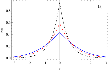
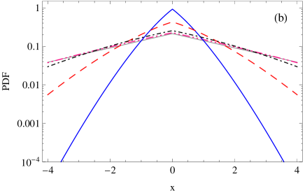
Figure 1: PDF (14) as function of $x$ for (a) time $t=1$ and resetting rates $r=0.1$ (blue solid line), $r=1$ (red dashed line), $r=5$ (black dot-dashed line); (b) $r=0.1$ and $t=0.1$ (blue solid line), $t=1$ (red dashed line), $t=5$ (black dot-dashed line), $t=10$ (violet dot-dot-dashed line), which approaches the stationary distribution (15) (solid thin grey line). We set $D_{x}=1$, $D_{y}=1$ and $U_{0}=1$.

From equation (12) we derive the MSD via the relation $\langle x^{2}(t)\rangle=\mathscr{L}^{-1}\left.\left\{-\partial^{2}\tilde{p}_{r,1}(k,s)/\partial x^{2}\right\}\right|_{k=0}$ [87]

$$\langle x^{2}(t)\rangle = 2\left(\frac{D_{x}}{2\sqrt{D_{y}}}\right)\mathscr{L}^{-1}\left\{s^{-1}\tilde{\eta}(s)\right\}$$ (20)

$$= \frac{D_{x}}{2D_{y}}U_{0}\frac{1-e^{-rt}}{r}-\frac{D_{x}}{2D_{y}}U_{0}\frac{e^{-rt}}{r}\mathrm{erf}\left(\frac{U_{0}}{2\sqrt{D_{y}}}\sqrt{t}\right)$$

$$+\frac{D_{x}}{2D_{y}}U_{0}\frac{\Delta_{r}}{r}\mathrm{erf}\left(\frac{U_{0}}{2\sqrt{D_{y}}}\Delta_{r}\sqrt{t}\right),$$

where $\Delta_{r}=\sqrt{1+4D_{y}r/U_{0}^{2}}$.

Let us consider two relevant limiting cases. In absence of confinement, $U_{0}=0$, the MSD reads

$$\langle x^{2}(t)\rangle=\frac{D_{x}}{\sqrt{D_{y}}}\frac{\mathrm{erf}\left(\sqrt{rt}\right)}{\sqrt{r}},$$ (21)

as it should be for diffusion in a comb with stochastic resetting in absence of a potential [84, 86]. Conversely, in the absence of resetting ($r=0$) the MSD (20) turns to

$$\langle x^{2}(t)\rangle=\frac{D_{x}}{2D_{y}}U_{0}\left[t+\frac{2\sqrt{D_{y}}}{U_{0}}\frac{t^{1/2}}{\Gamma(1/2)}\exp\left(-\frac{U_{0}^{2}}{4D_{y}}t\right)+\left(t+\frac{2D_{y}}{U_{0}^{2}}\right)\mathrm{erf}\left(\frac{U_{0}}{2\sqrt{D_{y}}}\sqrt{t}\right)\right],$$

which in the long time limit behaves as $\langle x^{2}(t)\rangle\simeq t$, also confirmed by the Gaussian PDF (19). This means that due to the confining potential along the branches the particle returns back to the backbone more frequently, resulting in normal diffusion along the $x$-axis. In this sense the confining potential is an integral part of the resetting mechanism. It is known that the stochastic resetting of a particle from the branch to the backbone also leads to normal diffusion along the $x$-axis [84]. An additional explanation of the confinment along the branches and resulting normal diffusion along the backbone is given in B.

From the final result (20) for the MSD we observe a saturation in the long time limit,

$$\langle x^{2}(t)\rangle\simeq\frac{D_{x}}{2D_{y}}U_{0}\frac{1+\Delta_{r}}{r},$$ (23)

which occurs due to the resetting of the particle, while in the short time limit, we observe the subdiffusive behaviour

$$\langle x^{2}(t)\rangle\sim 2\frac{D_{x}}{\sqrt{D_{y}}}\frac{t^{1/2}}{\Gamma(1/2)},$$ (24)

typical for free diffusion in a comb, since both resetting and potential do not affect the particle dynamics at short times. A graphical representation of the MSD is shown in figure 2. In figure 2(a) we observe the transition from subdiffusion, $\simeq t^{1/2}$, to the saturation plateau effected by resetting, for different values of the potential energy $U_{0}$. Figure 2(b) shows the behaviour of the MSD for fixed potential strength, $U_{0}=1$, and different values of the resetting rate $r$. For $r=0$ normal diffusion is observed in the long time limit (blue solid line), which occurs due to the confining potential in the fingers.

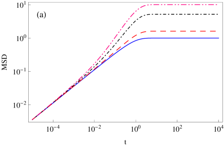
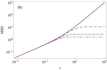
Figure 2: MSD (20) as function of time $t$ for (a) resetting rate $r=1$ and potential strength $U_{0}=0$ (blue solid line), $U_{0}=1$ (red dashed line), $U_{0}=5$ (black dot-dashed line), $U_{0}=10$ (violet dot-dot-dashed line); (b) for $U_{0}=1$ and $r=0$ (blue solid line), $r=0.1$ (red dashed line), $r=0.5$ (black dot-dashed line), $r=1$ (violet dot-dot-dashed line). We set $D_{x}=1$ and $D_{y}=1$.

We finally write down the Fokker-Planck equation for the marginal PDF along the branches, $p_{r,2}(y,t)=\int_{-\infty}^{\infty}p_{r}(x,y,t)\,dx$, in the form

$$\frac{\partial}{\partial t}p_{r,2}(y,t)=\left(\frac{\partial}{\partial y}V^{\prime}(y)+D_{y}\frac{\partial^{2}}{\partial y^{2}}\right)p_{r,2}(y,t)-r\,p_{r,2}(y,t)+r\delta(y),$$ (25)

which is the diffusion equation with resetting in presence of the confining potential [75].

3 Crossover to the steady state

We now analyse the crossover dynamics to the steady state. We rewrite the PDF (14) as follows

$$\tilde{p}_{r,1}(x,s) = \frac{1}{2}\sqrt{\frac{2\sqrt{D_{y}}}{D_{x}}}\frac{s^{-1}(s+r)\left(s+r+\frac{U_{0}^{2}}{4D_{y}}-\frac{U_{0}^{2}}{4D_{y}}\right)^{-1/2}}{\sqrt{\left(s+r+\frac{U_{0}^{2}}{4D_{y}}\right)^{1/2}+\frac{U_{0}}{2\sqrt{D_{y}}}}}$$

$$\times\exp\left(-\sqrt{\frac{2\sqrt{D_{y}}}{D_{x}}}{\left[\left(s+r+\frac{U_{0}^{2}}{4D_{y}}\right)^{1/2}-\frac{U_{0}}{2\sqrt{D_{y}}}\right]^{1/2}}|x-x_{0}|\right)$$

$$\equiv \tilde{p}_{0,1}(x,s+r+U_{0}^{2}/[4D_{y}])+s^{-1}r\tilde{p}_{0,1}(x,s+r+U_{0}^{2}/[4D_{y}]),$$

where we split the fraction $s^{-1}(s+r)$. Performing the inverse Laplace transform, we obtain

$$p_{r,1}(x,t)=\exp\left(-\left[r+\frac{U_{0}^{2}}{4D_{y}}\right]t\right)p_{0,1}(x,t)+\int_{0}^{t}r\exp\left(-\left[r+\frac{U_{0}^{2}}{4D_{y}}\right]t^{\prime}\right)p_{0,1}(x,t^{\prime})dt^{\prime}.$$

Here, $p_{0,1}(x,t)$ is given by

$$p_{0,1}(x,t)=\frac{1}{2}\sqrt{\frac{2\sqrt{D_{y}}}{D_{x}}}\mathscr{L}^{-1}\left\{\frac{\exp\left(-\sqrt{\frac{2\sqrt{D_{y}}}{D_{x}}}\left(s^{1/2}-\frac{U_{0}}{2\sqrt{D_{y}}}\right)^{1/2}|x-x_{0}|\right)}{\left(s-\frac{U_{0}^{2}}{4D_{y}}\right)^{1/2}\left(s^{1/2}+\frac{U_{0}}{2\sqrt{D_{y}}}\right)^{1/2}}\right\}.$$ (28)

This Laplace inversion of $p_{0,1}(x,t)$ for arbitrary $U_{0}\neq 0$ is not straightforward. However when $U_{0}=0$, this procedure is feasible. Therefore, for the clarity of the analysis we first consider this simplified case in absence of confinement in the branches. Then considering the simplified asymptotic form of the PDF $p_{0,1}(x,t)$ we will be able to compare with the difference in the presence of confinement, $U_{0}\neq 0$.

3.1 The case confinement-free branches ($U_{0}=0$)

In absence of the potential ($U_{0}=0$), the result of the Laplace inversion in equation (28) is exact and expressed in the form

$$p_{0,1}(x,t) = \frac{1}{2}\sqrt{\frac{2\sqrt{D_{y}}}{D_{x}}}\mathscr{L}^{-1}\left\{s^{-3/4}\exp\left(-\sqrt{\frac{2\sqrt{D_{y}}}{D_{x}}}s^{1/4}|x-x_{0}|\right)\right\}$$ (31)

$$= \frac{1}{2}\sqrt{\frac{2\sqrt{D_{y}}}{D_{x}}}t^{-1/4}H_{1,1}^{1,0}\left[\left.\sqrt{\frac{2\sqrt{D_{y}}}{D_{x}}}\frac{|x-x_{0}|}{t^{1/4}}\right|\begin{array}[]{l}(3/4,1/4)\\ (0,1)\end{array}\right],$$

where $H_{p,q}^{m,n}(z)$ is the Fox $H$-function [88]. Here we used the identity

$$e^{-z}=H_{0,1}^{1,0}\left[z\left|\begin{array}[]{l}-\\ (0,1)\end{array}\right.\right]$$ (32)

and the inverse Laplace transform

$$\mathscr{L}^{-1}\left\{s^{-\rho}H_{p,q}^{m,n}\left[a\,s^{\sigma}\left|\begin{array}[]{l}(a_{p},A_{p})\\ (b_{q},B_{q})\end{array}\right.\right]\right\}=t^{\rho-1}H_{p+1,q}^{m,n}\left[\frac{a}{t^{\sigma}}\left|\begin{array}[]{l}(a_{p},A_{p}),(\rho,\sigma)\\ (b_{q},B_{q})\end{array}\right.\right].$$ (37)

This density form can be employed to evaluate the distribution $p_{r,1}(x,t)$ in the presence of resetting,

$$p_{r,1}(x,t)=e^{-rt}p_{0,1}(x,t)+\int^{t}_{0}dt^{\prime}re^{-rt^{\prime}}p_{0,1}(x,t^{\prime}),$$ (39)

where the first term is given by equation (31) multiplied by $e^{-rt}$.

For further analysis it is convenient to use the asymptotic form for large argument of the Fox $H$-function in equation (31). We find the non-Gaussian form [89]

$$p_{0,1}(x,t)\sim\exp\left(-\frac{3}{2^{8/3}}\left[\frac{a|x-x_{0}|}{t^{1/4}}\right]^{4/3}\right).$$ (40)

Substituting this expression into the integral in the renewal equation (39) and focusing on the long time limit we have

$$\int_{0}^{t}e^{-rt^{\prime}}p_{0,1}(x,t^{\prime})dt^{\prime}\approx\int^{1}_{0}d\tau\exp\left(-t\,\Phi(\tau,|x-x_{0}|/t)\right),$$ (41)

where

$$\Phi(\tau,|x-x_{0}|/t)=r\tau+\frac{3a^{4/3}}{2^{8/3}}\left(\frac{|x-x_{0}|}{t}\right)^{4/3}\tau^{-1/3},\,\,\,a=\sqrt{2\sqrt{D_{y}}/D_{x}}.$$

We evaluate the integral in the Laplace approximation [90], which requires evaluation of the minimum of $\Phi$, defined as $0=\frac{d}{d\tau}\Phi|_{\tau=\tau_{0}}$, such that $\tau_{0}=\frac{1}{4r^{3/4}}\frac{a|x-x_{0}|}{t}$. Physically, this corresponds to the relaxation behavior of $p_{r,1}(x;t)$ with the saddle point $\tau_{0}$ determining the spatial region in which relaxation has been achieved, at time t. Outside the region the system is still in a transient state, and corresponds to the saddle point lying outside the unit interval. Thus, in the transient space-time region, the maximal contribution to the integral comes from the end point at $\tau=1$. Therefore, within this Laplace approximation, the large deviation form for the PDF $p_{r,1}(x,t)$ can be written as follows

$$p_{r,1}(x,t)\sim\exp\left(-t\,I_{r}\left(\frac{|x-x_{0}|}{t}\right)\right),$$ (43)

where the large deviation function is

$$I_{r}\left(\frac{|x-x_{0}|}{t}\right)=\left\{\begin{array}[]{ll}ar^{1/4}\frac{|x-x_{0}|}{t},&|x-x_{0}|<\frac{4r^{3/4}}{a}t,\\[5.69046pt] r+\frac{3a^{4/3}}{2^{8/3}}\left(\frac{|x-x_{0}|}{t}\right)^{4/3},&|x-x_{0}|>\frac{4r^{3/4}}{a}t.\end{array}\right.$$ (44)

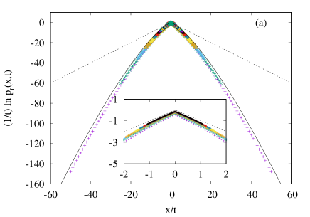
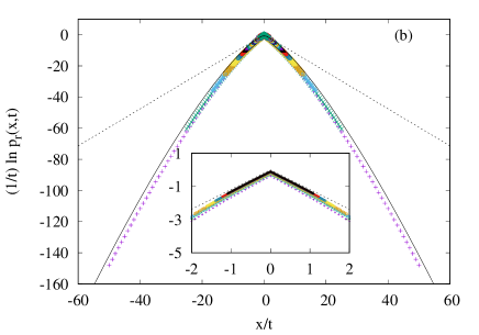
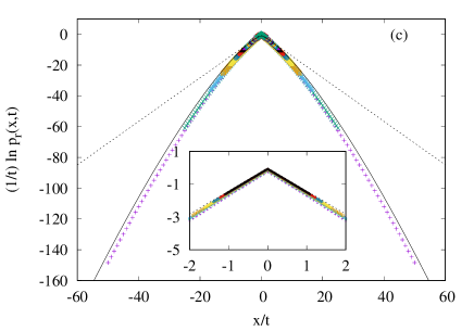
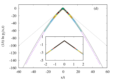
Figure 3: Logarithm of the PDF scaled by time, $(1/t)\log{p_{r,1}(x,t)}$, vs $x/t$ for (a) $r=1/4$, (b) $r=1/2$, (c) $r=1$, and (d) $r=2$. The data are obtained by numerical inverse Laplace transform of the PDF (LABEL:p1_final_laplace_U0_2) in Mathematica for $U_{0}=0$. The inset in the figures shows blow-up for small values of argument $|x|/t$. The black dotted line and the black solid lines indicate the two forms for the large deviation function $I_{r}$, see Eq. (44).

From the form of the large deviation function (44) it is evident that there occurs a qualitative change in the density profile $p_{r,1}(x,t)$ at a space-time point defined by $\tau_{0}<1$. This demarcates a “light-cone” region within which relaxation has been achieved and outside it the system is still relaxing. This relaxation behavior is, however, slower than the case of a Brownian motion relaxing to its nonequilibrium steady state under resetting [81]. The reason for this difference is that unlike Brownian motion on a line, a random walk on a two dimensional comb is subdiffusive ($U_{0}=0$). And hence, even though resetting is the common mechanism responsible for bringing about relaxation in both cases, the rate of relaxation, which is governed primarily by systemic details, is significantly different. Here we note that even though the stationary distribution in case of a diffusion in combs with resetting has been analysed before [84], this is the first time to explicitly find the corresponding large deviation function.

In order to verify our analytical estimates of the large deviation approximation of $p_{r}(x,t)$, we numerically invert the Laplace transform $\tilde{p}_{r}(x,s)$ for different values of the resetting rate $r$ as presented in figure 3. It is evident from the graphs that the numerical estimates very nicely corroborate our analytical results.

3.2 Presence of confinement in the branches ($U_{0}>0$)

In the presence of the confining potential, $U_{0}>0$, one cannot perform an analytical Laplace inversion of the PDF (LABEL:p1_final_laplace_U0_2). We therefore resort to numerical Laplace inversion of expression (LABEL:p1_final_laplace_U0_2), as shown in figure 4.

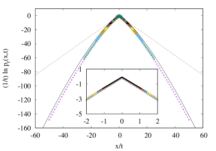
Figure 4: Logarithm of the PDF scaled by time, $(1/t)\log{p_{r,1}(x,t)}$, vs $x/t$, for $r=1$ and $U_{0}=1$. The black solid line and the black dotted line are drawn following a scaling form similar to the large deviation function in (44). It is to be noted, however, that these are numerically obtained results via analogy from the case $U_{0}=0$, see text.

In order to understand the result in figure 4 let us compare equations (3) and (39), which respectively are renewal equations for motion under resetting on a comb with and without confining branches. A careful inspection of the two equations makes it immediately evident that the confinement $U_{0}$ tends to modify the resetting rate $r$, except for the common prefactor of the integrals in (3) and (39). This is because both resetting and confinement have the effect of bringing the particle towards the backbone with one minor difference. Whereas resetting is instantaneous and takes the particle from anywhere on the comb to its initial location, the effect of confinement is non-instantaneous. The Brownian particle spends some time in its excursion along the branches before returning to the backbone. Furthermore, the location of return along the backbone due to confinement is not necessarily its initial location. Notwithstanding these slight differences, we see in figure 4 that the scaling function rendering the collapse of $p_{r,1}(x,t)$ at different times exhibits a behavior similar to case of nonconfining branches.

4 First-passage times along the backbone

We now turn to consider the first-time passage statistic along the backbone, by placing an absorbing boundary at $x=L>0$, i.e., $p_{1}(L,t)=0$. Without loss of generality we choose $x_{0}<L$. The equation of motion for the density function $p_{1}(x,t)$ in Laplace space along the backbone in absence of resetting follows from equation (8),

$$s\tilde{p}_{1}(x,s)-\delta(x-x_{0})=\frac{U_{0}D_{x}}{4D_{y}}(1+\Delta_{s})\frac{\partial^{2}\tilde{p}_{1}}{\partial x^{2}},$$ (45)

to be augmented with the boundary condition $p_{1}(L,t)=0$. We rephrase this expression as

$$\frac{\partial^{2}\tilde{p}_{1}}{\partial x^{2}}-As\tilde{p}_{1}=-A\delta(x-x_{0}),$$ (46)

where $A=4D_{y}/[U_{0}D_{x}(1+\Delta_{s})]$. Now, the auxiliary equation for the case $x\neq x_{0}$ for the above differential equation is $0=m^{2}-As$, implying $m=\pm\sqrt{As}$. We thus obtain

$$\tilde{p}_{1}(x,s)=\left\{\begin{array}[]{ll}b_{+}\exp\left(\sqrt{As}x\right)+b_{-}\exp\left(-\sqrt{As}x\right),&x<x_{0},\\[5.69046pt] c_{+}\exp\left(\sqrt{As}x\right)+c_{-}\exp\left(-\sqrt{As}x\right),&x>x_{0}.\end{array}\right.$$ (47)

Since $-\infty<x\leq L$ the requirement for physically meaningful solutions in the region $x<x_{0}$ is $b_{-}=0$. Continuity of the solution at $x=x_{0}$ and discontinuity of the derivative owing to the probability source at $x=x_{0}$ provide us with two relations between the parameters $b_{+}$ and $c_{\pm}$,

$$c_{+}\exp\left(\sqrt{As}x_{0}\right)+c_{-}\exp\left(-\sqrt{As}x_{0}\right)-b_{+}\exp\left(\sqrt{As}x_{0}\right) = 0,$$

$$c_{+}\exp\left(\sqrt{As}x_{0}\right)-c_{-}\exp\left(-\sqrt{As}x_{0}\right)-b_{+}\exp\left(\sqrt{As}x_{0}\right) = -\sqrt{A/s}.$$

In order to determine the value of these constants in terms of the system parameters we need one more relation, provided by the absorbing boundary condition at $x=L>x_{0}$, i.e., $\tilde{p}_{1}(L,s)=0$. Along with the previous two relations, this constraint fixes the parameters uniquely, and we obtain the density

$$\tilde{p}_{1}(x,s)=\left\{\begin{array}[]{ll}\displaystyle\sqrt{\frac{A}{s}}\sinh\left[\sqrt{As}(L-x_{0})\right]\exp\left(\sqrt{As}(x-L)\right),&x<x_{0},\\[11.38092pt] \displaystyle\sqrt{\frac{A}{s}}\sinh\left[\sqrt{As}(L-x)\right]\exp\left(\sqrt{As}(x_{0}-L)\right),&x>x_{0}.\end{array}\right.$$ (49)

Note that in the presence of the absorbing boundary the quantity $p_{1}(x,t)$ is no longer a PDF, as the cumulative (survival) probability becomes a decaying function of time. We then are in the position to derive the first-passage time density (FPTD)

$$\wp_{1}(t)=-\frac{d}{dt}\int_{-\infty}^{L}p_{1}(x,t)dx,$$ (50)

where the integral on the right hand side represents the survival probability. In Laplace domain,

$$\tilde{\wp}_{1}(s) = -\int^{L}_{-\infty}\Big{[}s\tilde{p}_{1}(x,s)-\delta(x-x_{0})\Big{]}dx=\left.-\frac{1}{A}\frac{\partial\tilde{p}_{1}}{\partial x}\right|_{x=L}$$ (51)

$$= \exp\left((x_{0}-L)\sqrt{\frac{4D_{y}s}{U_{0}D_{x}(1+\Delta_{s})}}\right),$$

where $\Delta_{s}=\sqrt{1+\frac{4sD_{y}}{U^{2}_{0}}}$. After Laplace inversion, the first-passage time reads

$$\wp_{1}(t) =\mathscr{L}^{-1}\left\{\exp\left(-\sqrt{\frac{4D_{y}s(\Delta_{s}-1)}{U_{0}D_{x}(\Delta_{s}^{2}-1)}}(L-x_{0})\right)\right\}$$

$$=\mathscr{L}^{-1}\left\{\exp\left(-\sqrt{\frac{U_{0}(\Delta_{s}-1)}{D_{x}}}(L-x_{0})\right)\right\}$$

$$=\mathscr{L}^{-1}\left\{\exp\left(-\sqrt{\frac{2\sqrt{D_{y}}}{D_{x}}}\left[\left(s+\frac{U_{0}^{2}}{4D_{y}}\right)^{1/2}-\frac{U_{0}}{2\sqrt{D_{y}}}\right]^{1/2}(L-x_{0})\right)\right\}.$$

For the long time limit, we find

$$\wp_{1}(t) \stackrel{{\scriptstyle[}}{{t}}\rightarrow\infty]{}{\sim}\left.\mathscr{L}^{-1}\left\{\exp\left(-\sqrt{\frac{2D_{y}}{D_{x}U_{0}}}(L-x_{0})s^{1/2}\right)\right\}\right|_{s\rightarrow 0}$$ (53)

$$\sim\mathscr{L}^{-1}\left\{1-\sqrt{\frac{2D_{y}}{D_{x}U_{0}}}(L-x_{0})s^{1/2}\right\}.$$

Therefore,

$$s^{-1}\tilde{\wp}_{1}(s) \stackrel{{\scriptstyle[}}{{s}}\to 0]{}{\sim}s^{-1}-\sqrt{\frac{2D_{y}}{D_{x}U_{0}}}(L-x_{0})s^{-1/2},$$ (54)

from where, by inverse Laplace transform, it follows that

$$\int_{0}^{t}\wp_{1}(t^{\prime})dt^{\prime}\sim 1-\sqrt{\frac{2D_{y}}{D_{x}U_{0}}}(L-x_{0})\frac{t^{-1/2}}{\Gamma(1/2)}\quad\rightarrow\quad\wp_{1}(t)\stackrel{{\scriptstyle[}}{{t}}\rightarrow\infty]{}{\sim}\sqrt{\frac{D_{y}}{2D_{x}U_{0}}}(L-x_{0})\frac{t^{-3/2}}{\Gamma(1/2)}.$$

A graphical representation of the FPTD is given in fiigure 5. It is evident that in the long time limit the FPTD behaves as $\wp_{1}(t)\simeq t^{-3/2}$

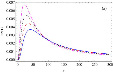
Figure 5: FPTD (LABEL:F1) as function of time $t$ for $D_{x}=1$, $D_{y}=1$, $U_{0}=1$, $L=10$ and $x_{0}=-1$ (blue solid line), $x_{0}=0$ (red dashed line), $x_{0}=1$ (black dot-dashed line) and $x_{0}=2$ (violet dot-dot-dashed line) (a) Linear-linear plot, (b) Log-log plot.

The mean first-passage time for normal diffusion on a semi-infinite line is infinite [55]. The same divergence will therefore occur in our comb structure for the motion along the semi-infinite domain on the backbone in absence of resetting. In that case we either have a crossover from subdiffusion to normal diffusion when the diffusion in the branches is confined ($U_{0}>0$), or continuing subdiffusion when there is no confinement, see also [52, 91]. Once we switch on the resetting dynamics, however, we expect the mean first-passage time to be finite. Using the results of [66] we find that expression (LABEL:F1) for the first-passage time density in absence of resetting helps us evaluate the mean first-passage time when resetting occurrs,

$$\langle T_{r}(x_{0})\rangle=\frac{1}{r}\left[\exp\left((L-x_{0})\sqrt{\frac{U_{0}}{D_{x}}(\Delta_{r}-1)}\right)-1\right],$$ (56)

where $\Delta_{r}=\sqrt{1+\frac{4rD_{y}}{U^{2}_{0}}}$. The divergence of the mean first-passage time in absence of resetting from this expression is obvious when we take the limit $r\to 0$. We also note the rapid growth of the mean first-passage time when the particle is rapidly reset to its initial location. In such a case the particle has an increasingly smaller chance to ever reach the absorbing boundary before the next reset. According to expression (56) the divergence of $\langle T_{r}(x_{0})\rangle$ corresponds to a pole of the form $1/r$ whereas the divergence for large $r$ is exponential. The non-monotonic behaviour of the mean first-passage time with the resetting rate is shown in figure 6 where we plot $\langle T_{r}(x_{0})\rangle$ as function of $\Delta_{r}$ for different (normalised) resetting locations $z=x_{0}/L$.

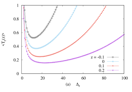
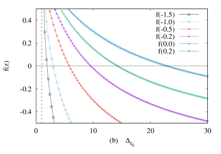
Figure 6: (a) Non-monotonic dependence of the mean first-passage time on the resetting rate $r$ and (b) zero-crossings of $f(z,x)=0$. The vertical dashed line in panel (b) indicates $\Delta_{r}=1$, signifying the fact that as the (normalised) resetting location $z=x_{0}/L$ approaches large negative values the optimal resetting rate $r_{0}$ approaches zero.

Apart from these immediate conclusions it is interesting to look at the behaviour of the mean first-passage time $\langle T_{r}(x_{0})\rangle$ as a function of the resetting rate $r$ in more detail. To this end we introduce two dimensionless quantities, $\tau_{0}=2D_{y}/U^{2}_{0}$ and $\mu=U_{0}L/(D_{x}/L)$ representing, respectively, a dimensionless time-scale and the ratio of the energy barrier to diffusion strength. Now, without any loss of generality we can choose the dimensionless time-scale as unity, i.e., $\tau_{0}=1$. In addition, as the orientations of the confining potential and the backbone are orthogonal to each other, we are at liberty to independently choose the values of $U_{0}$ and $D_{x}$. For simplicity we therefore choose $\mu=1$, without limiting generality. Then the mean first-passage time simplifies to

$$\langle T_{r}(z)\rangle=\frac{2}{\Delta^{2}_{r}-1}\left[\exp\left((1-z)\sqrt{\Delta_{r}-1}\right)-1\right],$$ (57)

where now $\Delta_{r}=\sqrt{1+2r}$. It is evident from this expression that the mean first-passage time to the absorbing wall in the presence of resetting exists for every $z\leq 1$ with $\langle T_{r}(1)\rangle=0$. The latter result is obvious, as the initial position coincides with the absorbing boundary. Expression (57) also allows the calculation of the optimal resetting rate $r_{0}$, at which the mean first-passage time is minimal, $\frac{d}{dr}\langle T_{r}(x_{0})\rangle|_{r=r_{0}}=0$, resulting in the transcendental equation

$$f(z)\equiv\frac{4\Delta_{r_{0}}}{(\Delta_{r_{0}}+1)\sqrt{\Delta_{r_{0}}-1}}\left[1-\exp\left(-(1-z)\sqrt{\Delta_{r_{0}}-1}\right)\right]-(1-z)=0,$$

which uniquely fixes $\Delta_{r_{0}}$ for a given value of $z$. Numerical analysis of this relation between the optimal $\Delta_{r_{0}}$ and function $f(z)$ for the corresponding resetting position $z$ as shown in figure 6 demonstrates that the optimal resetting rate $r_{0}$ approaches zero as the reset location $z$ takes large negative values. In other words, the optimal resetting rate exhibits a vanishing transition given that the mean first-passage time in absence of resetting is infinite.

5 Conclusions

SR is a phenomenon with almost ubiquitous relevance in a large range of systems, from diffusion controlled regulation in molecular biological processes to the search of higher animals for food. We here combined SR with the well established comb structure, a widely used model for loopless heterogeneous structures, with applications ranging from biologically relevant cases such as nerve fibres or blood vessels to aquifer backbones in groundwater dispersion. In our two-dimensional comb model we applied a confining potential of strength $U_{0}$, mimicking a finite length of the comb’s branches such that the mean residence time in these branches is kept finite. On top of the diffusivities $D_{x}$ and $D_{y}$ along the comb’s backbone and the branches, respectively, our system is therefore described by two additional relevant parameters, the confinement strength $U_{0}$ and the resetting rate $r$.

We demonstrated that while in absence of resetting a crossover occurs from initial subdiffusion to long time normal diffusion with Gaussian PDF (for the normal diffusion in absence of resetting see also an alternative viewpoint of the backbone diffusion in B), in the presence of resetting the initial subdiffusion eventually crosses over to a non-equilibrium steady state behaviour characterised by a plateau of the MSD. Depending on the choice of parameters, an intermediate normal diffusion regime may be observed. The PDF in the non-equilibrium steady state was shown to be of stretched exponential shape. We analysed the crossover dynamics to the steady state based on the large deviation function (44) using the asymptotic Laplace approximation method. This result also shows that the space-time region is now demarcated by a light-cone within which the system has relaxed to its nonequilibrium steady state, similar to the case of Brownian motion on a line. Outside this light-cone region, however, the rate of relaxation is slower in comparison to that of Brownian motion under resetting. This is because in the present geometry the particle tends to spend a finite amout of time along the branches rendering the relaxation, which is governed by the systemic details, to be achieved at a slower pace.

We also investigated the first-passage dynamics along the backbone. In particular we investigated the first-passage behaviour as function of the resetting rate and the amplitude of the confining potential. We calculated the mean first-passage time and the optimal resetting rate, at which the minimal first-passage time is obtained. Good agreement with a numerical evaluation is observed.

Appendix A Coupled Langevin equation approach and subordination

From equation (12) we find that the backbone’s marginal PDF satisfies

$$\tilde{p}_{1}(k,s)=\frac{\frac{1}{s\tilde{\eta}(s)}}{\frac{1}{\tilde{\eta}(s)}+\mathcal{D}k^{2}},$$ (59)

where $\mathcal{D}=\frac{D_{x}}{2\sqrt{D_{y}}}$. Alternatively, in integral form,

$$\tilde{p}_{1}(k,s) = \frac{1}{s\tilde{\eta}(s)}\int_{0}^{\infty}\exp\left(-u(1/\tilde{\eta}(s)+\mathcal{D}k^{2})\right)du$$ (60)

$$= \int_{0}^{\infty}e^{-u\mathcal{D}k^{2}}\tilde{h}(u,s)du,$$

where

$$\tilde{h}(u,s)=\frac{1}{s\tilde{\eta}(s)}e^{-u/\tilde{\eta}(s)}.$$ (61)

From inverse Fourier-Laplace transform we find [87]

$$p_{1}(x,t)=\int_{0}^{\infty}\frac{\exp(-x^{2}/[4\mathcal{D}u])}{\sqrt{4\pi\mathcal{D}u}}h(u,t)\,du.$$ (62)

The function $h(u,t)$ is called the subordinator which re-expresses the random process governed by the generalised diffusion equation (9) in physical time $t$ to the Wiener process with Gaussian PDF $f(x,u)=(4\pi\mathcal{D}u)^{-1/2}\exp\left(-x^{2}/[4\mathcal{D}u]\right)$, in terms of the operational time $u$.

This result can in fact be obtained from CTRW theory by considering the stochastic equations [92]

$$\left\{\begin{array}[]{ll}\frac{d}{du}x(u)=\xi(u),\\ \\ \frac{d}{du}T(u)=\zeta(u),\end{array}\right.$$ (66)

where $\xi(u)$ is a white Gaussian noise with zero mean and autocorrelation $\langle\xi(u)\xi(u^{\prime})\rangle=2\delta(u-u^{\prime})$ while $\zeta(u)$ is a completely one-sided Lévy stable noise. This means that the random walk $x(t)$ is parametrised in terms of the ”number of steps” $u$. The inverse process $S(t)$ of the Lévy process $T(u)$ with characteristic function $\langle\exp(-sT(u))\rangle=\exp(-\Psi(s)u)$ represents a collection of first-passage times, $S(t)=\inf\{u>0:T(u)>t\}$ [92]. Then the CTRW can be defined by the subordinated process $X(t)=x(S(t))$. The PDF $h(u,t)$ of the inverse process $S(t)$ can be found from the relation [92]

$$h(u,t)=-\frac{\partial}{\partial u}\langle\Theta(t-T(u))\rangle,$$ (67)

where $\Theta(z)$ is the Heaviside step function. Laplace transform then yields

$$\tilde{h}(u,s) = -\frac{\partial}{\partial u}\frac{1}{s}\left<\int_{0}^{\infty}\delta(t-T(u))e^{-st}dt\right>$$ (68)

$$= -\frac{\partial}{\partial u}\frac{1}{s}\langle e^{-sT(u)}\rangle=-\frac{\partial}{\partial u}\frac{1}{s}e^{-\Psi(s)u}=\frac{\Psi(s)}{s}e^{-\Psi(s)u}.$$

Therefore,

$$p_{1}(x,t)=\langle\delta(x-X(t))\rangle=\langle\delta(x-X(S(t))\rangle=\int_{0}^{\infty}f(x,u)h(u,t)dt,$$ (69)

from where one can easily arrive at the generalised diffusion equation (9), when $\tilde{\Psi}(s)=1/\tilde{\eta}(s)$, where $\tilde{\eta}(s)$ is given by equation (10). The corresponding CTRW model represents a random process with Gaussian jump length PDF and waiting time PDF in the Laplace domain of the form $\tilde{\psi}(s)=(1+1/\tilde{\eta}(s))^{-1}\sim 1-1/\tilde{\eta}(s)$.

Appendix B Confinement along the branches

As a result of confinement along the branches, the particle tends to exhibit a normal diffusive transport along the backbone at longer times. Furthermore the potential along the $y$-axis branches results in a steady-state

$$p_{0,2,st}(y)\simeq\exp\left(-\frac{U_{0}}{D_{y}}|y|\right).$$ (70)

If we look at distribution of the maxima of excursions along the $y$-branch, then

$$P(M_{n}\geq y)=P(Y_{1}\geq y,\ldots,Y_{n}\geq y)=[P(Y\geq y)]^{n}\sim\exp\left(-\left[\frac{nU_{0}}{D}\right]y\right),$$ (71)

which implies that the maximal excursions along the confining branches are exponentially distributed. In other words, the confinement effectively confined diffusion in branch regions of finite length [31].

References

References

- [1] J. M. Sancho, A. M. Lacasta, K. Lindenberg, I. M. Sokolov, and A. H. Romero, Phys. Rev. Lett. 92, 250601 (2004).
- [2] E. M. Lifshitz and L. P. Pitaevskii, Landau and Lifshitz Course on Theoretical Physics: Physical Kinetics, Butterworth-Heinemann, London, UK (1981).
- [3] N. G. van Kampen, Stochastic Processes in Physics and Chemistry, North-Holland, Amsterdam (1981).
- [4] J.-P. Bouchaud and A. Georges, Phys. Rep. 195, 127 (1990).
- [5] M. J. Saxton, Biophys. J. 92, 1178 (2007).
- [6] R. Metzler, J.-H. Jeon, A. G. Cherstvy, and E. Barkai, Phys. Chem. Chem. Phys. 16, 24128 (2014).
- [7] F. Höfling and T. Franosch, Rep. Progr. Phys. 76, 046602 (2013).
- [8] K. Nørregaard, R. Metzler, C. Ritter, K. Berg-Sørensen, and L. Oddershede, Chem. Rev. 117, 4342 (2017).
- [9] R. Metzler and J. Klafter, Phys. Rep. 339, 1 (2000).
- [10] J.-H. Jeon, N. Leijnse, L. B. Oddershede, and R. Metzler, New J. Phys. 15, 045011 (2013).
- [11] D. T. Gillespie, Am. J. Phys. 64, 225 (1996).
- [12] A. Caspi, R. Granek, and M. Elbaum, Phys. Rev. Lett. 85, 5655 (2000).
- [13] K. Chen, B. Wang, and S. Granick, Nat. Mater. 14, 589 (2015).
- [14] M. S. Song, H. C. Moon, J.-H. Jeon, and H. Y. Park, Nat. Commun. 9, 344 (2018).
- [15] M. F. Shlesinger, B.West, and J. Klafter, Phys. Rev. Lett. 58, 1100 (1987).
- [16] P. Siegle, I. Goychuk, and P. Hänggi, Phys. Rev. Lett. 105, 100602 (2010).
- [17] E. Baskin and A. Iomin, Phys. Rev. Lett. 93, 120603 (2004).
- [18] S. Singh, R. K. Singh, and S. Kumar, Phys. Rev. E 102, 012605 (2020).
- [19] B. Wang, J. Kuo, S. C. Bae, and S. Granick, Nat. Mater. 11, 481 (2012).
- [20] R. Metzler, Euro. Phys. J. Special Topics 229, 711 (2020).
- [21] T. Sandev, A. Iomin, and L. Kocarev, Phys. Rev. E 102, 042109 (2020).
- [22] V. Stojkoski, T. Sandev, L. Basnarkov, L. Kocarev, and R. Metzler, Entropy 22, 1432 (2020); V. Stojkoski, T. Sandev, L. Kocarev, and A. Pal, arXiv:2104.01571.
- [23] T. Sandev, V. Domazetoski, A. Iomin, and L. Kocarev, Mathematics 9, 221 (2021).
- [24] A. G. Cherstvy and R. Metzler, Phys. Chem. Chem. Phys. 15, 20220 (2013).
- [25] Y. G. Sinai, Theor. Probab. Appl. 27, 256 (1982).
- [26] A. Godec, A. V. Chechkin, E. Barkai, H. Kantz, and R. Metzler, J. Phys. A: Math. Theor. 47, 492002 (2014).
- [27] B. B. Mandelbrot, The Fractal Geometry of Nature, Freeman, San Francisco CA (1982).
- [28] D. ben-Avraham and S. Havlin, Diffusion and Reactions in Fractals and Disordered Systems, Cambridge University Press, Cambridge (2000).
- [29] J. Feder, Fractals, Plenum Press, New York, NY (1988).
- [30] T. A. L. Ziman, J. Phys. C: Solid State Phys. 12, 2645 (1979).
- [31] S. R. White and M. Barma, J. Phys. A: Math. Gen. 17, 2995 (1984).
- [32] Y. Gefen and I. Goldhirsch, J. Phys. A: Math. Gen. 18, L1037 (1985).
- [33] G. H. Weiss and S. Havlin, Physica A 134, 474 (1986).
- [34] V. E. Arkhincheev and E. M. Baskin, Zh. Eskp. Teor. Fiz. 100, 292 (1991); V. E. Arkhincheev and E. M. Baskin, Sov. Phys. JETP 73, 161 (1991).
- [35] F. Santamaria, S. Wils, E. De Schutter, and G. J. Augustine, Neuron 52, 635 (2006).
- [36] S. Fedotov and V. Méndez, Phys. Rev. Lett. 101, 218102 (2008).
- [37] V. Méndez and A. Iomin, Chaos, Solitons & Fractals 53, 46 (2013).
- [38] A. Biess, E. Korkotian, and D. Holcman, Phys. Rev. E 76, 021922 (2007).
- [39] F. Colaiori, A. Flammini, A. Maritan, and J. R. Banavar, Phys. Rev. E 55, 1298 (1997).
- [40] A. Rinaldo, A. Marani, and R. Rigon, Wat. Res. Res. 27, 513 (1991).
- [41] J. W. Kirchner, X. Feng, and C. Neal, Nature 403, 524 (2000).
- [42] H. Scher, G. Margolin, R. Metzler, J. Klafter, and B. Berkowitz, Geophys. Res. Lett. 29, 1061 (2002).
- [43] A. Iomin, Phys. Rev. E 83, 052106 (2011).
- [44] E. K. Lenzi, T. Sandev, H. V. Ribeiro, P. Jovanovski, A. Iomin, and L. Kocarev, J. Stat. Mech. 2020, 053203 (2020).
- [45] V. Méndez, A. Iomin, W. Horsthemke, and D. Campos, J. Stat. Mech. 2017, 063205 (2017).
- [46] T. Sandev, A. Iomin, H. Kantz, R. Metzler, and A. Chechkin, Math. Model. Nat. Phenom. 11, 18 (2016).
- [47] A. Iomin, Phys. Rev. E 86, 032101 (2012).
- [48] H. V. Ribeiro, A. A. Tateishi, L. G. A. Alves, R. S. Zola, and E. K. Lenzi, New J. Phys. 16, 093050 (2014).
- [49] A. Iomin, V. Méndez, and W. Horsthemke, Fractal Fract. 3, 54 (2019).
- [50] Y. He, S. Burov, R. Metzler, and E. Barkai, Phys. Rev. Lett. 101, 058101 (2008).
- [51] J. H. P. Schulz, E. Barkai, and R. Metzler, Phys. Rev. X 4, 011028 (2014).
- [52] M. R. Evans and S. N. Majumdar, Phys. Rev. Lett. 106, 160601 (2011).
- [53] M. R. Evans and S. N. Majumdar, J. Phys. A: Math. Theor. 47, 285001 (2014).
- [54] S. Eule and J. Metzger, New J. Phys. 18, 033006 (2016).
- [55] S. Redner, A Guide to First Passage Processes, Cambridge University Press, Cambridge (2001).
- [56] R. Metzler, S. Redner, and G. Oshanin, editors, First-passage Phenomena and their Applications, World Scientific, Singapore (2014).
- [57] A. J. Bray, S. N. Majumdar, and G. Schehr, Adv. Phys. 62, 225 (2013).
- [58] A. Godec and R. Metzler, Phys. Rev. X 6, 041037 (2016).
- [59] D. Grebenkov, R. Metzler, and G. Oshanin, Comm. Chem. 1, 96 (2018).
- [60] G. Kolesov, Z. Wunderlich, O. N. Laikova, M. S. Gelfand, and L. A. Mirny, Proc. Natl. Acad. Sci. USA 104, 13948 (2007).
- [61] O. Pulkkinen and R. Metzler, Phys. Rev. Lett. 110, 198101 (2013).
- [62] J. Ma, M. Do, M. A. Le Gros, C. S. Peskin, C. A. Larabell, Y. Mori, and S. A. Isaacson, PLoS Comp. Biol. 16, e1008356 (2020).
- [63] A. Falcón-Cortés, D. Boyer, L. Giugiolli, and S. N. Majumdar, Phys. Rev. Lett. 119, 140603 (2017).
- [64] A. Pal, L. Kuśmierz, and S. Reuveni, Phys. Rev. Res. 2, 043174 (2020).
- [65] A. Pal and S. Reuveni, Phys. Rev. Lett. 118, 030603 (2017).
- [66] S. Reuveni, Phys. Rev. Lett. 116, 170601 (2016).
- [67] A. Chechkin and I. M. Sokolov, Phys. Rev. Lett. 121, 050601 (2018).
- [68] A. S. Bodrova, A. V. Chechkin, and I. M. Sokolov, Phys. Rev. E 100, 012120 (2019).
- [69] A. S. Bodrova, A. V. Chechkin, and I. M. Sokolov, Phys. Rev. E 100, 012119 (2019).
- [70] C. Christou and A. Schadschneider, J. Phys. A: Math. Theor. 48, 258003 (2015).
- [71] A. Pal and V. V. Prasad, Phys. Rev. E 99, 032123 (2019).
- [72] S. Ray, D. Mondal, and S. Reuveni, J. Phys. A: Math. Theor. 52, 255002 (2019); D. Gupta, A. Pal, and A. Kundu, J. Stat. Mech. 2021, 043202 (2021).
- [73] S. Ray and S. Reuveni, J. Chem. Phys. 152, 234110 (2020).
- [74] A. Pal, Phys. Rev. E 91, 012113 (2015); A. Pal, L. Kuśmierz, and S. Reuveni, New J. Phys. 21, 113024 (2019).
- [75] R. K. Singh, R. Metzer, and T. Sandev, J. Phys. A 53, 505003 (2020).
- [76] A. Pal, A. Kundu, and M. R. Evans, J. Phys. A: Math. Theor. 49, 225001 (2015); A. Masó-Puigdellosas, D. Campos, and V. Méndez, Phys. Rev. E 100, 042104 (2019).
- [77] M. R. Evans and S. N. Majumdar, J. Phys. A: Math. Theor. 44, 435001 (2011).
- [78] L. Kuśmierz, S. N. Majumdar, S. Sabhapandit, and G. Schehr, Phys. Rev. Lett. 113, 220602 (2014).
- [79] D. Campos and V. Méndez, Phys. Rev. E 92, 062115 (2015).
- [80] S. Ahmad, I. Nayak, A. Bansal, A. Nandi, and D. Das, Phys. Rev. E 99, 022130 (2019).
- [81] S. N. Majumdar, S. Sabhapandit, and G. Schehr, Phys. Rev. E 91, 052131 (2015).
- [82] M. Dahlenburg, A. V. Chechkin, R. Schumer, and R. Metzler, arXiv:2104.14866.
- [83] M. R. Evans, S. N. Majumdar, and G. Schehr, J. Phys. A: Math. Theor. 53, 193001 (2020).
- [84] V. Domazetoski, A. Masó-Puigdellosas, T. Sandev, V. Méndez, A. Iomin, and L. Kocarev, Phys. Rev. Res. 2, 033027 (2020).
- [85] S. C. Lim and S. V. Muniandy, Phys. Rev. E 66, 021114 (2002).
- [86] A. A. Tateishi, H. V. Ribeiro, T. Sandev, I. Petreska, and E. K. Lenzi, Phys. Rev. E 101, 022135 (2020); M. A. F. Dos Santos, Fractal Fract. 4, 28 (2020).
- [87] T. Sandev, I. M. Sokolov, R. Metzler, and A. Chechkin, Chaos, Solitons & Fractals 102, 210 (2017); T. Sandev, R. Metzler, and A. Chechkin, Fract. Calc. Appl. Anal. 21, 10 (2018).
- [88] A. M. Mathai, R. K. Saxena, and H. J. Haubold, The -function: Theory and Applications, Springer, New York (2010).
- [89] G. Rangarajan and M. Ding, Phys. Rev. E 62, 120 (2000).
- [90] G. B. Arfken and H. J. Weber, Mathematical Methods for Physicists, 6th ed. Elsevier Academic Press (2005).
- [91] R. Metzler and J. Klafter, J. Phys. A: Math. Gen. 37, R161 (2004).
- [92] H. C. Fogedby, Phys. Rev. E 50, 1657 (1994).