Pushing the limits of time beyond the Big Bang singularity: Scenarios for the branch cut universe

Abstract

In this contribution we identify two scenarios for the evolutionary branch cut universe. In the first scenario, the universe evolves continuously from the negative complex cosmological time sector, prior to a primordial singularity, to the positive one, circumventing continuously a branch cut, and no primordial singularity occurs in the imaginary sector, only branch points. In the second scenario, the branch cut and branch point disappear after the realisation of the imaginary component of the complex time by means of a Wick rotation, which is replaced by the thermal time. In the second scenario, the universe has its origin in the Big Bang, but the model contemplates simultaneously a mirrored parallel evolutionary universe going backwards in the cosmological thermal time negative sector. A quantum formulation based on the WDW equation is sketched and preliminary conclusions are drawn.

1 The illusion of time

Newton’s conception of the clockwork universe, evolving like a mechanical perfect clock and whose movements of its gears are governed by the laws of physics, with an inherent predictability, prevailed for more than three centuries, until a revolutionary concept emerged, thanks to the genius mind of Hermann Minkowski(Minkowski, 1915), with profound consequences for our current understanding of its structure and evolution.

According to his view, instead of being considered separate entities (though intimately related), space and time were combined into a single continuum entity, the spacetime.

Time in physics is usually considered a fundamental variable, defined by its measurement as the reading of a clock. In opposition to this view, John Weeler and Bryce DeWitt developed in 1967 the so called WdW equation (DeWitt, 1967) based on the audacious idea of physics without time, a theoretical framework that sought to combine quantum mechanics and general relativity, representing a step towards a consistent theory of quantum gravity.

More recently, Carlo Rovelli affirmed that the flow of time is an illusion and that our naive perception of it doesn’t correspond to physical reality (Rovelli, 2019), a vision that is in tune with Albert Einstein’s perception of time. Carlos Rovelli also recently revisited the idea of ‘physics without time’ (Rovelli, 2004; Rovelli  Smerlak, 2011; Rovelli, 2015) bearing in mind that, in accordance with the second law of thermodynamics, forward in time is the direction in which entropy increases, and in which we gain information, so the flow of time is a subjective feature of the universe, not an objective part of physical reality. In this realm, in which the observable universe does not show time reversal symmetry, events, rather than particles or fields, are the basic constituents of the universe, and the task of physics would be to describe the relationship between events.

These conceptions present some points of contact with a line of thought we recently developed (Vasconcellos ., 2020, 2021) where we applied the tools of singular semi-Riemannian geometry to push the limits of general relativity and time beyond a primordial singularity, giving rise to a branch cut universe. In this contribution we sought to identify evolutionary scenarios for the branch cut universe.

2 Wick rotation of cosmological time

Wick rotation is a well known theoretical method that encapsulates a connection between quantum mechanics and quantum statistical mechanics and in another ground relativistic field theory in Minkowski spacetime manifolds and Euclidean field theory in Riemannian spacetime manifolds.

2.1 Path integral formalism

The path integral formalism (Feynman  Hibbs, 1965) describes the quantum transition amplitudes of the unitary time evolution operator, $\hat{U}(t_{\rm{b}},t_{\rm{a}})$ (a representation of the abelian group of time translations), between the localised quantum mechanical states of a particle ($x_{a},t_{\rm{a}}$) to ($x_{b},t_{\rm{b}}$), with $x$ and $t$ denoting space and time Cartesian coordinates. The matrix elements of the quantum time evolution amplitudes, using bra’s ($\langle x_{b}|$) and ket’s ($|x_{a}\rangle$) notation, read

$$(x_{b}t_{\rm{b}}|x_{a}t_{\rm{a}})=\langle x_{b}|\hat{U}(t_{\rm{b}},t_{\rm{a}})|x_{a}\rangle\,\,t_{\rm{b}}>t_{\rm{a}}\,,$$ (1)

For a system with a time-independent Hamiltonian operator, $\hat{H}$, the time evolution operator is simply

$$\hat{U}(t_{\rm{b}},t_{\rm{a}})=\hat{\bar{\tau}}e^{-\frac{i}{\hbar}\hat{H}(t_{\rm{b}}-t_{\rm{a}})}\,,$$ (2)

where $\hat{\bar{\tau}}$ denotes the time-ordering operator. In the continuum limit, we write the amplitude $(x_{b}t_{\rm{b}}|x_{a}t_{\rm{a}})$ as a path integral

$$(x_{b}t_{\rm{b}}|x_{a}t_{\rm{a}})\equiv\int_{x_{a}}^{x_{b}}{\cal D}_{x}e^{i{\cal A}(x)/\hbar}\,.$$ (3)

This equation is the corresponding Feynman’s formula for the quantum-mechanical amplitude (1) and represents the sum over all paths in configuration space with a phase factor containing the action ${\cal A}[x]$.

2.2 Wick rotation in statistical and quantum mechanics

In statistical mechanics, the quantum partition function $Z(T)$, which contains all information about the thermodynamical equilibrium properties of a quantum system, reads

$$Z(T)\equiv Tr\Bigl{(}e^{-\hat{H}/k_{B}T}\Bigr{)}\equiv Tr\Bigl{(}e^{-H(\hat{p},\hat{x})/k_{B}T}\Bigr{)}\,.$$ (4)

In this expression, $Tr(\hat{F})$ denotes the trace of the operator

$$\hat{F}=e^{-H(\hat{p},\hat{x})/k_{B}T}\,,$$ (5)

and $k_{B}$ is the Boltzmann constant. For a $N$-particle system described by the Schrödinger equation for instance, the quantum-statistical system refers to a canonical ensemble.

The quantum statistical partition function $Z(T)$ may be related to the quantum-mechanical time evolution operator $Z_{QM}(t_{\rm{b}}-t_{\rm{a}})$

$$Z_{QM}(t_{\rm{b}}-t_{\rm{a}})\equiv Tr\Bigl{[}\hat{U}(t_{\rm{b}},t_{\rm{a}})\Bigr{]}=Tr\Bigl{[}e^{-i(t_{\rm{b}}-t_{\rm{a}})\hat{H}/\hbar}\Bigr{]}\,,$$ (6)

by making an analytical continuation of the time interval $t_{\rm{b}}-t_{\rm{a}}$ to the negative imaginary value using a Wick rotation:

$$t_{\rm{b}}-t_{\rm{a}}\rightarrow-i\hbar/k_{B}T\,.$$ (7)

In quantum mechanics and quantum field theory, the Hamiltonian density ${\cal H}$ acts as the generator of the Lie group of time translations while in statistical mechanics the Hamiltonian represents a Boltzmann weight in an ensemble. The contour-rotation from the real to the imaginary time-axis, results in a correspondence between the imaginary time component and the inverse of the temperature, $T$ and it can be understood as a realisation of the imaginary component of time.

2.3 Euclidean quantum gravity

Euclidean quantum gravity refers to a quantum theory of Riemannian manifolds in which the quantisation of gravity occurs in a Euclidean spacetime, generated by means of a Wick rotation. The corresponding gravitational path integral in the presence of a field $\phi$ may be expressed as

$${\cal Z}=\int{\cal D}[g]{\cal D}[\phi]e^{\int d^{4}x\sqrt{|{\mathbf{g}}|}\,R}\,.$$ (8)

Additional assumptions imposed to the manifolds as compactness, connectivity and boundaryless (no singularities), make this formulation a strong candidate for overcoming the limitations presented by general relativity in the domain of strong gravity, more precisely, the elimination of singularities in extreme physical conditions. There are other techniques that sought to overcome these limitations of general relativity. Among these, we highlight the pseudo-complex general relativity, a very powerful technique based on pseudo-complex spacetime coordinates (Hess ., 2015; Hess, 2017; Hess  Boller, 2020) with observational predictions given in (Schönenbach ., 2014).

3 Cosmography in an universe with a branch cut

The tracking of the analytically continued scale factor $\ln^{-1}[\beta(t)]$ and the background cosmological Hubble rate $H_{\rm{ac}}(t)$, analytically continued to the complex plane enable us to trace the evolutive paths of the branch cut universe from its initial stages to the present days (for the details see Vasconcellos . (2021)).

The scale factor $\ln^{-1}[\beta(t)]$, a dimensionless quantity, describes the change in sizes of portions of space (or patches) due to the expansion or contraction of the branch cut universe. The Hubble parameter $H_{\rm{ac}}(t)$ in turn measures the expansion rate of the branch cut universe. We assume the observable universe corresponds today to a patch of space with radius $R(t_{0})$, and that the patch size of the branch cut universe at any other period of time is given by

$$\frac{\ln^{-1}[\beta(t)]}{\ln^{-1}(\beta_{0})}R(t_{0})=\frac{\ln(\beta_{0})}{\ln[\beta(t)]}R(t_{0})\,.$$ (9)

3.1 Cosmological parameters

The analytically continued energy-stress conservation law in the expanding universe may be written as (for the details see Vasconcellos . (2021)):

$$\frac{1}{\rho(t)}\frac{d}{dt}\rho(t)\!+\!3\Bigl{(}\!1+\frac{p(t)}{c^{2}\rho(t)}\!\Bigr{)}\frac{1}{\ln^{-1}[\beta(t)]}\frac{d\ln^{-1}[\beta(t)]}{dt}$$ (10)

$$\!\Rightarrow\!\frac{d}{dt}\ln(\rho(t))\!+\!3\Bigl{(}1+\frac{p(t)}{c^{2}\rho(t)}\Bigr{)}\frac{d}{dt}\ln[\ln^{-1}[\beta(t)]\!=\!0.$$

From this equation it results

$$\rho(t)=\rho_{0}exp\Biggl{(}-2\int\epsilon(t)d\!\!\ln\,(\ln^{-1}[\beta(t)])\Biggr{)}\,,$$ (11)

where

$$\epsilon(t)\equiv\frac{3}{2}\Bigl{(}1+\frac{p(t)}{c^{2}\rho(t)}\Bigr{)}\,,$$ (12)

represents a dimensionless thermodynamical connection between the energy density $\rho(t)$ and pressure $p(t)$ of a perfect fluid thus enabling the fully description of the equation of state (EoS) of the system. Positive pressure corresponds to $\epsilon>3/2$, negative pressure to $\epsilon<3/2$ and for a universe dominated by a cosmological constant, $\epsilon\to 0$.

In the limit in which the dimensionless thermodynamical connection obeys $\epsilon(t)\to\epsilon=$ constant, the integral (11) reduces to

$$\ln[\rho(t)/\rho_{0}] = -2\lim_{\epsilon(t)\to\epsilon}\int\epsilon(t)\,d\!\!\ln(\ln^{-1}[\beta(t)])$$ (13)

$$\simeq -2\epsilon\ln(\ln^{-1}[\beta(t)])\Rightarrow\ln\,(\ln^{-1}[\beta(t)])^{-2\epsilon}$$

$$\Rightarrow \rho(t)\simeq\frac{\rho_{0}}{\ln^{-2\epsilon}[\beta(t)]}\,,$$

which corresponds to an analytically continued expression for the density of the branch cut universe. Applying complex conjugation to this expression we get

$$\rho^{*}(t^{*})=\frac{\rho^{*}_{0}}{\ln^{-2\epsilon}(\beta^{*}(t^{*}))}\,.$$ (14)

3.2 Horizons and cosmological curvatures

An event’s causality is limited to its frontal light cone since information cannot travel faster than the speed of light. Light rays travel in null geodesics, so the following expressions results for the analytically continued (ac) co-moving (cm), ${\cal D}^{\rm{cm}}_{\rm{ac}}(t)$, and proper (p), ${\cal D}^{\rm{p}}_{\rm{ac}}(t)$, distances to the horizon:

$${\cal D}^{\rm{cm}}_{\rm{ac}}(t)=\int_{t_{\rm{P}}}^{t}\frac{cdt}{\ln^{-1}[\beta(t)]}\,;\,\,\,{\cal D}^{\rm{p}}_{\rm{ac}}(t)=\ln^{-1}[\beta(t)]\int_{t_{\rm{P}}}^{t}\frac{cdt^{\prime}}{\ln^{-1}[\beta(t^{\prime})]}\,.$$ (15)

We also develop expressions for the analytically continued time-dependent and dimensionless cosmic curvature factor (ccf), $\Omega^{\rm{ccf}}_{\rm{ac}}(t)$ (apparent spatial curvature), and the cosmic anisotropy factor (caf), $\Omega^{\rm{caf}}_{\rm{ac}}(t)$ (apparent anisotropy):

$$\Omega^{\rm{ccf}}_{\rm{ac}}(t)\!=\!-\frac{kc^{2}}{\ln^{-2}[\beta(t)]}H_{\rm{ac}}^{-2}(t)\,;\,\,\,\Omega^{\rm{caf}}_{\rm{ac}}(t)\!=\!\frac{\sigma^{2}}{\ln^{-6}[\beta(t)]}H_{\rm{ac}}^{-2}(t)\,.$$ (16)

Combining these expressions with the definition of $H_{\rm{ac}}$ (Vasconcellos ., 2021), we get

$$\Omega^{\rm{ccf}}_{\rm{ac}}(t)=-\frac{k\beta^{2}(t)}{\dot{\beta}^{2}(t)\ln^{-4}[\beta(t)]}\,;\,\,\,\Omega^{\rm{caf}}_{\rm{ac}}(t)=\frac{\sigma^{2}\beta^{2}(t)}{\dot{\beta}^{2}(t)\ln^{-8}[\beta(t)]}.$$ (17)

Applying complex conjugation to these expressions we obtain

$$\Omega^{*\rm{ccf}}_{\rm{ac}}(t^{*})=-\frac{k\beta^{*2}(t^{*})}{\dot{\beta}^{*2}(t^{*})\ln^{-4}[\beta^{*}(t^{*})]}\,,$$ (18)

$$\mbox{and}\,\,\,\,\Omega^{*\rm{caf}}_{\rm{ac}}(t^{*})=\frac{\sigma^{*2}\beta^{*2}(t^{*})}{\dot{\beta}^{*2}(t^{*})\ln^{-8}[\beta^{*}(t^{*})]}\,.$$ (19)

In appendix A, we present solutions for the cosmography parameters in a branch cut universe.

3.3 Cosmological Redshift

Light emitted by distant objects from our galaxy travels from the point of emission at $t=t_{\rm{e}}$, $r=r_{\rm{e}}$ to the observation point today $t=t_{\rm{o}}$, $r=r_{\rm{o}}$ along the geodesic curves of a manifold, which correspond essentially to local straight lines ($d\theta\sim d\phi\sim 0$), satisfying $ds_{\xi}^{2}=0$.

The line element of the modified FLWR metric of a three-dimensional spatial slice of an analytically continued spacetime, in co-moving coordinates may be written as

$$ds_{\xi}^{2}=c^{2}dt_{\xi}^{2}-a_{\xi}^{2}(t)\left(\frac{dr_{\xi}^{2}}{1-k\,r_{\xi}^{2}}+r_{\xi}^{2}\Bigl{[}d\theta^{2}+\sin^{2}\theta\,d\phi^{2}\Bigr{]}\right).$$ (20)

The conditions $d\theta\sim d\phi\sim 0$ and $ds_{\xi}^{2}=0$ applied to this equation allows the mapping (Vasconcellos ., 2020, 2021)

$$\rightarrow c^{2}dt_{\xi}^{2}-a_{\xi}^{2}(t)\frac{dr_{\xi}^{2}}{1-k\,r_{\xi}^{2}}=0\stackrel{{\scriptstyle}}{{\longrightarrow}}\frac{1}{1+z_{\rm{ac}}}\equiv\frac{\ln^{-1}[\beta(t)]}{\ln^{-1}(\beta_{0})},$$ (21)

$$\longrightarrow z_{\rm{ac}}\equiv\frac{\ln[\beta(t)]-\ln(\beta_{0})}{\ln(\beta_{0})}\,;$$

$z_{\rm{ac}}$ represents the analytically continued cosmological corresponding to the metric (20), $t$ denotes the proper time measured by a co-moving observer and the radial and angular coordinates in the co-moving frame are represented by $r$, $\theta$ and $\phi$. From equation (21), variations of $z_{\rm{ac}}$, more specifically $\Delta z$ obey

$$\Delta z_{\rm{ac}}=\frac{\ln[\beta(t)]/\beta_{0}}{ln(\beta_{0})}\,.$$ (22)

A Taylor expansion of the analytically continued Hubble’s law for two objects at a distance $d$ apart gives:

$$\ln^{-1}[\beta(t)] = \ln^{-1}(\beta_{0})+\frac{d}{dt}\Bigl{(}\ln^{-1}[\beta(t)]\Bigr{)}\Bigr{|}_{t=t_{0}}\Bigl{(}t-t_{0}\Bigr{)}$$ (23)

$$+ \frac{1}{2}\frac{d^{2}}{dt^{2}}\Bigl{(}\ln^{-1}[\beta(t)]\Bigr{)}\Bigr{|}_{t=t_{0}}\Bigl{(}t-t_{0}\Bigr{)}^{2}+\cdot\cdot\cdot$$

On small scales, the distance to an emitter, $d$ is approximately related to the time of emission, $t$, so we can then rewrite (21) as

$$\frac{1}{1+z_{\rm{ac}}}-H_{\rm{ac}0}\frac{d}{c}-\frac{q_{\rm{ac}0}}{2}H^{2}_{\rm{ac}0}\Bigl{(}\frac{d}{c}\Bigr{)}^{2}+\cdot\cdot\cdot$$ (24)

with $\ln^{-1}(\beta_{0})$ normalised to $1$ and where

$$q_{\rm{ac}0}=-\frac{\Bigl{(}\frac{d^{2}}{dt^{2}}\ln^{-1}[\beta(t)]\Bigr{)}\ln^{-1}[\beta(t)]}{\bigl{(}\frac{d}{dt}\ln^{-1}[\beta(t)]\bigr{)}^{2}}\,,$$ (25)

represents the analytically continued deceleration parameter. On small scales and at small redshifts we obtain the analytically continued Hubble’s law,

$$cz_{\rm{ac}}=H_{\rm{ac}0}d\,.$$ (26)

4 On the road of a quantum approach

The challenge of building a quantum theory of gravitation based on the simple combination of quantum mechanics and general relativity, due to their so distinct characteristics, is significant. In the following we present a few remarks about the physical and geometric meaning of $\ln^{-1}[\beta(t)]$ and $\beta(t)$ and we sketch first steps on the road of a quantum approach for the branch cut universe.

4.1 The problem of time

It is believed that general relativity and quantum mechanics should be reconciled in a theory of quantum gravity, merging at the Planck scale. It is also believed that the spacetime geometry cannot be measured below the Planck scale (Garay, 1999; Calmet ., (2004), since quantum spacetime fluctuations would spoil at this scale its description as a smooth spacetime manifold (Garay, 1999).

The essential difference between quantum mechanics and general relativity that makes their reconciliation extremely difficult is the interpretation and the role of time. In quantum mechanics, time corresponds to a universal and absolute parameter. As a consequence, the formal treatment of time in quantum mechanics differs from the other coordinates that may be raised to the category of quantum operators and observables. In general relativity, in turn, time is said to be malleable and relative (Isham, 1993). As a consequence, unification of quantum mechanics and general relativity requires reconciling their absolute and relative notions of time.

4.2 Wheeler-DeWitt Equation

An illuminating example is the formulation and interpretation of the Wheeler-DeWitt (WdW) equation (DeWitt, 1967). The Wheeler-DeWitt formulation for quantum gravity consists in constraining a wave function which applies to the universe as a whole, — the so called wave function of the universe —, in accordance with the Dirac recipe:

$$\hat{\cal H}\Psi=0\,,$$ (27)

i.e., a stationary, timeless equation, instead of a time-dependent quantum mechanics wave equation as for instance

$$i\frac{\partial}{\partial t}\hat{H}\Psi\,.$$ (28)

Here, $\hat{H}$ denotes the Hamiltonian operator of a quantum subsystem, while $\hat{\cal H}$ in the previous equation represents a quantum operator which describes a general relativity constraining, resulting in a second order hyperbolic equation of gravity variables, a Klein-Gordon-type equation, having therefore a ‘natural’ conserved associated current (${\cal J}$),

$${\cal J}=\frac{i}{2}\Bigl{(}\Psi^{\dagger}\,\nabla\cdot\Psi-\Psi\,\nabla\cdot\Psi^{\dagger}\Bigr{)};\,\,\,\mbox{with}\,\,\nabla\cdot{\cal J}=0\,.$$ (29)

Primordial technical deficiencies have historically led to a tendency to underestimate the WdW equation as a consistent formulation of quantum gravity, despite supporting several approaches, from quantum geometrodynamics to loop quantum gravity. More recently, however, an opposite trend has emerged, related to the understanding of the fundamental reasons for the intriguing explicit absence of the time variable in the WdW equation, i.e., that the time variable has no physical significance in general relativity (Rovelli  Smerlak, 2011; Rovelli, 2015; Shestakova, 2018). Based on this understanding, in the following we sketch a quantum formulation of the present approach based on the WdW equation analytically continued to the complex plane.

4.3 Analytically continued WdW equation

4.3.1 Einstein-Hilbert action in the new metric

The define the analytically continued FLRW metric (Vasconcellos ., 2021):

$$ds_{[\rm{ac}]}^{2}=-\sigma^{2}N^{2}(t)c^{2}dt^{2}+\sigma^{2}\ln^{-2}[\beta(t)]d\Omega^{2}(r,\theta,\phi)\,,$$ (30)

with

$$d\Omega^{2}(r,\theta,\phi)\equiv\Biggl{[}\frac{dr^{2}}{\bigl{(}1-kr^{2}(t)\bigr{)}}+r^{2}(t)\Bigl{(}d\theta^{2}+sin^{2}\theta d\phi^{2}\Bigr{)}\Biggr{]}.$$ (31)

In expression (30), $N(t)$ is an arbitrary lapse function, and $\sigma^{2}=2/3\pi$ is just a normalisation factor.

We assume as a starting point a homogeneous and isotropic multiverse described by a mini-superspace model (see for instance Kim (1997)) with only one dynamical variable, the scale factor $\ln^{-1}[\beta(t)]$, and a very simple scenario for the Einstein-Hilbert action $S_{\rm{EH}}$ (He  Cai, 2020)

$$S_{\rm{EH}} = \frac{1}{16\pi G}\int{\cal L}\,dtd^{3}x$$ (32)

$$= \frac{1}{16\pi G}\int\sqrt{-g}\Bigl{(}R_{[gac]}c^{3}-\frac{16\pi G\rho}{\sigma^{2}c}\Bigr{)}dtd^{3}x\,,$$ (33)

where $R_{[gac]}$ represents the analytically continued scalar curvature (for the details see Vasconcellos . (2021)):

$$R_{[gac]} = 6\Biggl{[}\Biggl{(}\frac{\frac{d^{2}}{dt^{2}}{\ln^{-1}[\beta(t)]}}{\sigma^{2}c^{2}N^{2}(t)\ln^{-1}[\beta(t)]}\Biggr{)}$$ (34)

$$+ \Biggl{(}\frac{\frac{d}{dt}{\ln^{-1}[\beta(t)]}}{\sigma cN(t)\ln^{-1}[\beta(t)]}\Biggr{)}^{2}+\frac{k}{\sigma^{2}\ln^{-2}[\beta(t)]}\Biggr{]},$$

and $\rho$ represents the energy density of the multiverse.

Combining (32) and (34) and using the approximation $\sqrt{-g}\approx N(t)\ln^{-3}[\beta(t)]$, we obtain

$$S \!=\! \int\frac{6\sigma^{2}N(t)c^{4}}{16\pi G}\Biggl{(}\frac{\ln^{-2}[\beta(t)]}{N^{2}(t)c^{2}}\frac{d^{2}}{dt^{2}}\ln^{-1}[\beta(t)]$$

$$\!+\! \ln^{-1}[\beta(t)]\Biggl{[}\!\Bigl{(}\!\frac{\frac{d}{dt}\ln^{-1}[\beta(t)]}{N(t)c}\!\Bigr{)}^{2}+k\!\Biggr{]}\!-\!\frac{8\pi G\rho}{3c^{4}}\ln^{-3}[\beta(t)]\!\Biggr{)}\,d^{4}x.$$

We integrate this equation by parts to remove the second derivative in $\ln^{-1}[\beta(t)]$, resulting in

$$S=\frac{Nc^{4}}{2G}\int\Biggl{(}\!\!\!\! - \ln^{-1}[\beta(t)]\Bigl{(}\frac{\frac{d}{dt}\ln^{-1}[\beta(t)]}{Nc}\Bigr{)}^{2}$$

$$+ k\ln^{-1}[\beta(t)]-\frac{8\pi G\rho}{3c^{4}}\ln^{-3}[\beta(t)]\!\Biggr{)}dt\,.$$

Making the choice $N=G=c=1$ (see footnote 6), from this equation we obtain the Lagrangian density of the multiverse:

$${\cal L}=\frac{1}{2}\Biggl{(}k\ln^{-1}[\beta(t)]\, - \,\ln^{-1}[\beta(t)]\Bigl{(}\frac{d}{dt}\ln^{-1}[\beta(t)]\Bigr{)}^{2}$$ (37)

$$- \,\frac{8\pi\rho}{3}\ln^{-3}[\beta(t)]\Biggr{)}.$$

In the following, on basis of this Lagrangian formulation, we proceed with the quantisation of the system.

4.4 Topological Quantisation

The conjugate momentum $p_{\rm{\ln}}$ of the dynamical variable $\ln^{-1}[\beta(t)]$ is

$$p_{\rm{\ln}}=\frac{\partial{\cal L}}{\partial\bigl{(}\frac{d}{dt}\ln^{-1}[\beta(t)]\bigr{)}}=-\ln^{-1}[\beta(t)]\frac{\dot{\beta}(t)}{\beta(t)}\,.$$ (38)

Therefore the corresponding Hamiltonian becomes

$${\cal H} = p_{\rm{\ln}}\frac{d}{dt}\ln^{-1}[\beta(t)]-{\cal L}\,,$$

$$= -\frac{1}{2}\Biggl{(}\frac{p^{2}_{\ln}}{\ln^{-1}[\beta(t)]}+k\ln^{-1}[\beta(t)]+\frac{8\pi\rho}{3}\ln^{-3}[\beta(t)]\Biggr{)}\,.$$

The quantisation of the Lagrangian density is achieved by raising the dynamical variable $\ln^{-1}[\beta(t)]$ and the conjugate momentum $p_{\rm{\ln}}$ to the category of operators in the form

$$\ln^{-1}[\beta(t)]\rightarrow\hat{\ln}^{-1}[\beta(t)]\,$$ (40)

$$\mbox{and}\,\,p_{\rm{\ln}}\rightarrow\widehat{p}_{\rm{\ln}}=-i\hbar\frac{\partial}{\partial\ln^{-1}[\beta(t)]};$$

(for simplicity, in the following we skip using the hat symbol in the operators $\hat{\rm{p}}$ and $\hat{\ln}$). Ambiguities in ordering of the operators may be overcome by the introduction of an ordering-factor $\alpha$ in the form

$$p^{2}=-\frac{1}{\ln^{-\alpha}}\frac{\partial}{\partial\ln^{-1}[\beta(t)]}\Biggl{(}\ln^{-\alpha}[\beta(t)]\frac{\partial}{\partial\ln^{-1}[\beta(t)]}\Biggr{)}\,,$$ (41)

with $\alpha$ usually chosen in general as $\alpha=[0,1]$; $\alpha=0$ corresponds to the semiclassical value; intermediate values have no meaning.

Combining (4.4) and (41), using the prescription $\alpha=0$, recovering the original values of the physical constants $G$ and $c$, and changing variable ($u\equiv\ln^{-1}[\beta(t)]$ and $du\equiv d\ln^{-1}[\beta(t)]$) we obtain the following expression for the WdW equation:

$$\Biggl{(}-\frac{\hbar^{2}}{2m_{\rm{P}}}\frac{\partial^{2}}{\partial u^{2}}+\frac{E_{\rm{P}}k}{2\ell^{2}_{\rm{P}}}u^{2}-\frac{4\pi\rho}{3\ell_{\!\!P}}u^{4}\Biggr{)}\Psi(u)=0\,,$$ (42)

where $m_{\rm{P}}$, $E_{\rm{P}}$, and $\ell_{\rm{P}}$ are the Planck mass, energy and length, respectively (for comparison see for instance He  Cai (2020)). This expression represents a Schrödinger-type equation of a particle with the Planck mass $m_{\rm{P}}$ under the action of the WdW quantum potential

$${\cal V}_{[\rm{ac}]\rm{WdW}}\bigl{(}\ln^{-1}[\beta(t)]\bigr{)}=\frac{E_{\rm{P}}k}{2\ell^{2}_{\rm{P}}}\ln^{-2}[\beta(t)]-\frac{4\pi\rho}{3\ell_{\!\!P}}\ln^{-4}[\beta(t)])\,.$$ (43)

4.4.1 Topological quantisation of spacetime

The scale factor $\ln^{-1}[\beta(t)]$ as the only dynamical variable of the model may be raised, in a quantum approach, at the level of a quantum operator. This new status gives the scale factor $\ln^{-1}[\beta(t)]$ an additional role in describing the evolutionary process of the branch cut universe, that of representing the formal confluence between the classic description and its quantum version through a process that we call spacetime topological quantisation, as far as we know, a new nomenclature which characterises a new perspective in the quantisation of spacetime. Our formulation describes in short the relative evolution of the variable $\ln^{-1}[\beta(t)]$ over worldlines $\gamma_{\rm{\ln}}$ associated with hypersurfaces ${\cal H}_{\rm{\ln}}$ analytically continued to the complex plane.

4.5 Analytically continued WdW equation

In the following we consider an extended version of the analytically continued WdW equation (42) with extrinsic curvature contributions implemented by using the projectable Hořava-Lifshitz gravity model:

$$\Bigl{(}-\frac{\partial^{2}}{\partial u^{2}}+{\cal V}_{\rm{WdWHL}}(u)\Bigr{)}\Psi(u)=0\,,$$ (44)

with

$${\cal V}_{\rm{WdWHL}}(u)=\Bigl{(}2{\cal V}_{[\rm{ac}]\rm{WdW}}(u)+{\cal V}_{\rm{HL}}(u)\Bigr{)}\,,$$ (45)

where ${\cal V}_{\rm{HL}}(u)$ represents an adaptation of the Hořava-Lifshitz gravity potential:

$${\cal V}_{\rm{HL}}(u)=g_{c}k-g_{\Lambda}u-\frac{g_{r}k^{2}}{u}-\frac{g_{s}k}{u^{2}}\,;$$ (46)

(for comparison see Bertolami  Zarro (2011); Cordero . (2019); He  Cai (2020)). Here, $g_{C}>0$, stands for the curvature coupling constant with the sign of $g$ following the sign of the cosmological constant (Bertolami  Zarro, 2011); $g_{r}$ corresponds to the coupling constant for the radiation contribution and $g_{s}$ stands for the “stiff” matter contribution (which corresponds to the $\rho=p$ equation of state); $g_{r}$ and $g_{s}$ can be either positive or negative since their signal does not alter the stability of the Hořava-Lifshitz gravity (Bertolami  Zarro, 2011).

Combining (42), (44), (45), and (46), the following equation results:

$$\Biggl{(}\!\!-\frac{\partial^{2}}{\partial u^{2}}+g_{c}k-g_{\Lambda}u+ku^{2}-\frac{8\pi\rho}{3}u^{4}-\frac{g_{r}k^{2}}{u}-\frac{g_{s}k}{u^{2}}\!\!\Biggr{)}\Psi(u)\!=\!0.$$ (47)

This equation, when expressed in terms of non-composed functions, as in the conventional quantum FLRW approach, is highly non-linear and has no exact solution.

4.5.1 Solutions

Assuming the first two terms of the potential given by (47), $g_{c}k$ and $-g_{\Lambda}u$, are dominant, the substitution

$$\xi\Rightarrow(g_{\Lambda})^{-2/3}\bigl{(}g_{c}k-g_{\Lambda}u\bigr{)},$$ (48)

leads to an Airy equation:

$$\Biggl{(}\frac{\partial^{2}}{\partial\xi^{2}}-\xi\Biggr{)}\Psi(\xi)=0,$$ (49)

whose solution is

$$\Psi(\xi)=C_{1}Ai(\xi)+C_{2}B(\xi)\,,$$ (50)

where $Ai(\xi)$ and $B(\xi)$ are the Airy functions of the first and second kind, respectively. The system of equations also supports complex conjugated solutions:

$$\Psi^{*}(\xi^{*})=C^{*}_{1}Ai^{*}(\xi^{*})+C^{*}_{2}B^{*}(\xi^{*})\,.$$ (51)

4.5.2 Boundary Conditions

The evolution phases of the universe can lead to different combinations of pressure and density characterised by different values of the dimensionless thermodynamical connection $\epsilon(t)$ (12). In the following, however, for simplicity we chose a symmetric evolution description of the universe for positive and negative cosmological time.

It is expected that the most appropriate solutions of the WdW equation give rise, in the late universe, to a classic spacetime, and provide an initial condition for the inflationary period, necessary for the resolution of the flatness and horizon problems of classical cosmology. To meet these expectations, it is crucial to impose appropriate boundary conditions to the WdW equation. Here, as a first sketch of our quantum proposal, we do not enter in those specific aspects and impose the following boundary conditions:

$$\lim_{\xi\to-\infty}\Psi(-\xi)\to 0\,;\lim_{\xi\to\infty}\Psi(\xi)\to 0\,.$$ (52)

5 Results

In Fig. (1) we show characteristic plots of the Riemann surface associated to the real parts of $\ln[\beta(t)]$ and $\ln[1/\beta(t)]$, assuming that $\beta(t)$ is a orthomodular function. Fig. (2)shows the corresponding plots of $\ln^{-1}[\beta(t)]$ and $\ln^{-1}[1/\beta(t)]$.

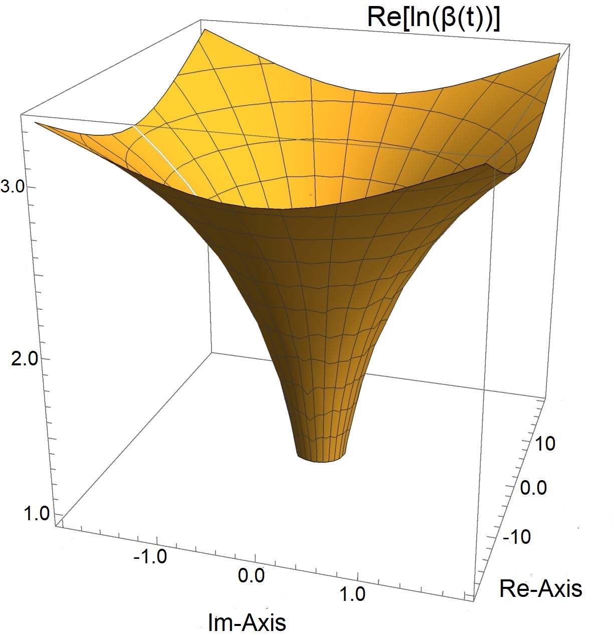
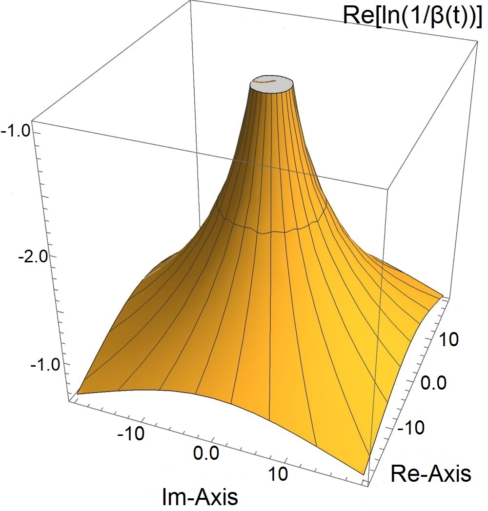
Figure 1: Left figure: Characteristic plot of the Riemann surface $R$ associated to the real part of the $\ln[\beta(t)]$ function, represented by $Re[\ln[\beta(t)]]$, limited to one Riemann sheet in the region surrounding the Planck scale, the transition region corresponding to the domain where general relativity and quantum mechanics reconcile. Right figure: Plot of the real part of the $Re[\ln[1/\beta(t)]]$, assuming that the $\beta(t)$ function is orthomodular. The domain of the quantum leap is indicated in the figure.

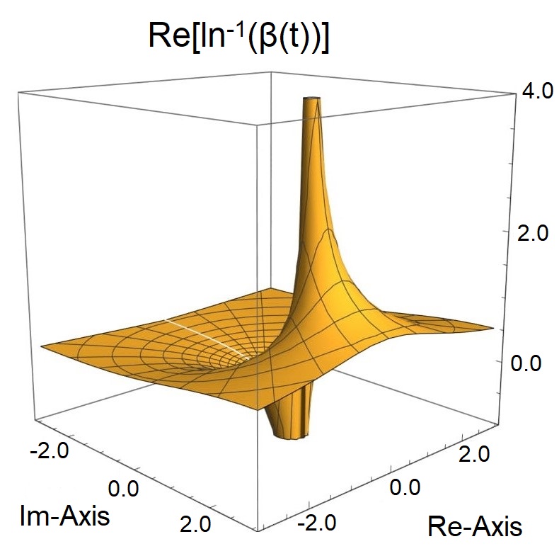
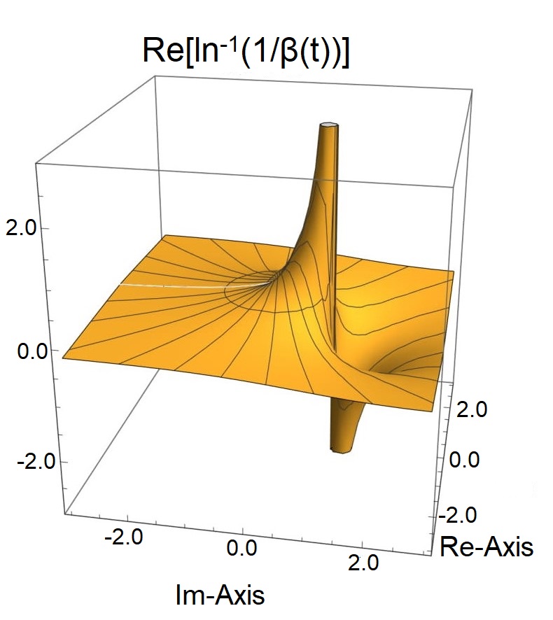
Figure 2: Left figure: Characteristic plot of the Riemann surface $R$ associated to the real part of the $\ln^{-1}[\beta(t)]$ function, represented by $Re[\ln^{-1}[\beta(t)]]$ limited to one Riemann sheet in the region surrounding the Planck scale. Right figure: Plot of the real part of the inverse of the previous figure, $Re[\ln^{-1}[1/\beta(t)]]$.

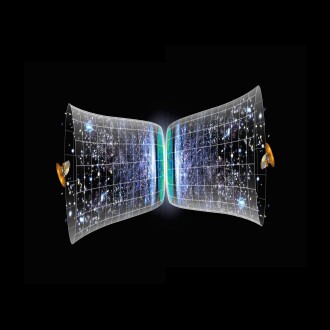
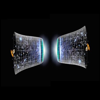
Figure 3: Left figure shows an artistic representation of the branch cut universe evolution with two scenarios. The figures were based on the artistic impressions by ESO / M. Kornmesser (Kornmesser, 2020).

5.1 Scenarios for the branch cut universe

Our previous results delineate two scenarios for the evolution of the branch cut universe which are sketched in an artistic representation (see Fig. (3)), with a branch point and a branch cut on the left figure, and no primordial singularity on the right one. The figures indicate the cosmic contraction and expansion phases of the branch cut universe. In the representation sketched on the left figure, the branch cut universe evolves from negative to positive values of the complex cosmological time $t_{C}$, — or the thermal time $T$, as a result of a Wick rotation —, circumventing continuously a a branch cut and no primordial singularity occurs, only branch points. The right figure on (3) sketches an alternative artistic representation of two mirrored evolving universes, originated both from primordial singularities. As an example, in Fig. (4) characteristic plots of the unnormalised solutions of equation (50), for the first scenario, are shown.

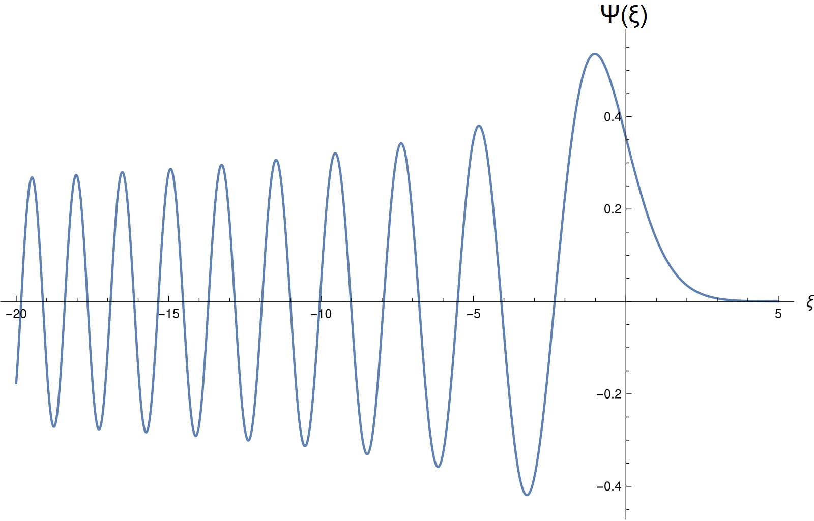
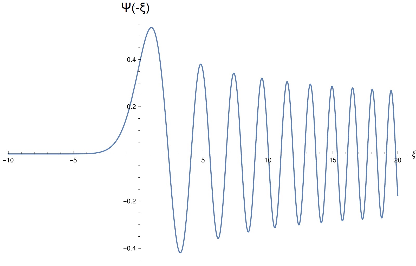
Figure 4: Characteristic solution of equation (50).

6 Discussion

The first scenario of the branch cut universe is characterised by its continuous expansion and by a systematic decrease of the temperature in its positive complex cosmological time sector. In the second scenario, the branch cut and branch point disappear after the realisation of imaginary time by means of a Wick rotation, which is replaced here by the real and continuous thermal time (temperature). In this second scenario, a mirrored parallel evolutionary universe, adjacent to ours, is nested in the structure of space and time, with its evolutionary process going backwards in the cosmological thermal time negative sector. In this case, the connection between the previous solutions is broken as a result of the Wick rotation. A similar result may be obtained if we adopt an approach based on the path integral formalism with no singularity in the first scenario. In the first scenario the entropy decreases systematically and continuously in the negative thermal time sector until the absolute zero of entropy was reached. And then follows the increase of the entropy systematically in the positive thermal time sector. In the second scenario, entropy increases systematically in the evolution process of our universe but in the parallel mirror-universe, the arrow of time points down the entropy gradient, so the entropy is negative (negentropy sector).

Our sketched quantised formulation, based on the Wheeler De Witt equation, brings an alternative ingredient to overcoming the primordial singularity of the universe. In particular, the solutions of the quantised version (50) are in line with the description of the first scenario. A more detailed and in-depth discussion of these aspects involving both scenarios requires a more detailed future analysis.

6.0.1 Observational signatures

An expressive challenge is the observational realisation of the proposal presented. Speculations associated with the birth of two universes during the Big Bang, above 13.5 billion years ago, - our universe and another one, which from our perspective is functioning in reverse with time running backward —, as well as the multiverse conception are known and recurring. Fictional literature is lavish in this type of narrative, and from the scientific point of view, there are renowned scientists who are skeptical of the conception, and others who are proponents of multiverse theories, as S. Hawking for instance.

Observations that may give some shelter to such conceptions are very rare or nonexistent. Interpretations of observational data based on such hypotheses were quickly demystified. More recently, the Antarctic Impulsive Transient Antenna ANITA/NASA project has detected for the second time (Gorham ., 2018) a fountain of high-energy particles that resembles an upside-down cosmic-ray shower, generating a pleiades of speculations about the meaning of these observations and the possible realisation of a universe specular to ours. Although not supported by the authors of the article, speculations still persist. From our perspective, the formalism presented here represents a mathematical resource with a view to overcoming singularities in general relativity.

7 Final remarks

As stressed before (Vasconcellos ., 2021), the present formalism presents similarity with quantum bouncing models which assume in general a mechanism (or trigger) to keep the bouncing phase stable which could be associated for example with quantum fluctuations. In this kind of quantum bouncing models, the contraction phase amplifies quantum fluctuations and could serve as a trigger for the expansion phase (see for instance Novello  Bergliaffa (2008)). In turn, the quantum formulation sketched in this contribution represents a kind of quantum tunnelling between the contraction and the expansion phases, an effect quite similar to the corresponding tunnelling effect in ordinary quantum mechanics.

Using the causal structure of the McVittie spacetime (McVittie, 1933) for a classical bouncing cosmological model, Pérez . (2021) recently found out that when the universe reaches a certain minimum scale, the trapping horizons disappear and the black hole ceases to exist, suggesting that neither a contracting nor an expanding universe can accommodate a black hole at all times. In our view, the formalism presented here could represent a solution for the survival of black holes from the contraction sector to the expanding one. The model presented by  Pérez . (2021) contains a fundamental ingredient for such description, the scale factor $a(t)$ that can be analytically continued to the complex space, thus enabling a transition from the contraction phase, in which the universe reaches a certain minimum scale that causes the trapping horizons to disappear and the black hole ceases to exist to the expansion phase. An investigation into this topi c is ongoing.

In physics, the prevailing tendency among scientists is to think of space and time as constituting the central structure of the universe. Conceptions as physics without time and about the flow of time being an illusion have enriched the debate about its meaning. A question then arises: how to reconcile these visions with the remarkable predictions of general relativity that implies a materialisation of spacetime, such as in the detection of gravitational waves, conceived as ‘ripples’ in spacetime? We obviously do not intend to have a definitive answer to this question. As a final word, as we see, speculations on this still open questions find a fertile sea in another Einstein’s quotation (Hedman, 2017): ‘time and space are modes by which we think and not conditions in which we live’, a statement so powerful and profound that it will certainly continue to enlighten our creativity and imagination.

8 Acknowledgements

P:O:H: acknowledges financial support from PAPIIT-DGAPA (IN100421). The authors wish to thank the referees for valuable comments.

Appendix A Cosmography parameters

In the following we show our results for the analytically continued cosmography parameters for the radiation-, matter-, and dark-matter dominated eras.

A.1 Radiation-dominated era

For the radiation-dominated era, we obtain

$$\rho(t)\simeq\frac{\rho_{0}}{\sqrt[2\epsilon]{\ln^{-2}[\beta(t_{\rm{P}})]+\frac{1}{\ln^{\,2}(\beta_{0})}\sqrt{\frac{2\pi G\rho_{0}}{3}}\Bigl{(}t-t_{\rm{P}}\Bigr{)}}}.$$ (53)

Similarly,

$$\rho^{*}(t^{*})\simeq\frac{\rho^{*}_{0}}{\sqrt[2\epsilon]{\ln^{-2}[\beta(t_{\rm{P}}^{*})]+\frac{1}{\ln^{\,2}(\beta_{0})}\sqrt{\frac{2\pi G\rho_{0}}{3}}\Bigl{(}t^{*}-t_{\rm{P}}^{*}\Bigr{)}}}.$$ (54)

Additionally, we have

$$\Omega_{\rm{ccf}}(t)=-\frac{3k\ln^{\,4}(\beta_{0})}{\pi G\rho_{0}}\frac{\ln^{2}\sqrt{\ln^{-2}[\beta(t_{\rm{P}})]+\frac{1}{\ln^{\,2}(\beta_{0})}\sqrt{\frac{2\pi G\rho_{0}}{3}}\Bigl{(}t-t_{\rm{P}}\Bigr{)}}}{\Bigl{(}\ln^{-2}[\beta(t_{\rm{P}})]+\frac{1}{\ln^{\,2}(\beta_{0})}\sqrt{\frac{2\pi G\rho_{0}}{3}}\bigl{(}t-t_{\rm{P}}\bigr{)}\Bigr{)}}\,,$$

and

$$\Omega_{\rm{caf}}(t)=\frac{3\sigma^{2}\ln^{\,4}(\beta_{0})}{\pi G\rho_{0}}\frac{\ln^{2}\sqrt{\ln^{-2}[\beta(t_{\rm{P}})]+\frac{1}{\ln^{\,2}(\beta_{0})}\sqrt{\frac{2\pi G\rho_{0}}{3}}\Bigl{(}t-t_{\rm{P}}\Bigr{)}}}{\Bigl{(}\ln^{-2}[\beta(t_{\rm{P}})]+\frac{1}{\ln^{\,2}(\beta_{0})}\sqrt{\frac{2\pi G\rho_{0}}{3}}\bigl{(}t-t_{\rm{P}}\bigr{)}\Bigr{)}^{4}}\,.$$

Similarly,

$$\Omega^{*}_{\rm{ccf}}(t^{*})=-\frac{3k\ln^{\,4}(\beta^{*}_{0})}{\pi G\rho^{*}_{0}}\frac{\ln^{2}\sqrt{\ln^{-2}[\beta(t^{*}_{\rm{P}})]+\frac{1}{\ln^{\,2}(\beta^{*}_{0})}\sqrt{\frac{2\pi G\rho^{*}_{0}}{3}}\Bigl{(}t^{*}-t^{*}_{\rm{P}}\Bigr{)}}}{\Bigl{(}\ln^{-2}[\beta(t^{*}_{\rm{P}})]+\frac{1}{\ln^{\,2}(\beta^{*}_{0})}\sqrt{\frac{2\pi G\rho^{*}_{0}}{3}}\bigl{(}t^{*}-t^{*}_{\rm{P}}\bigr{)}\Bigr{)}}\!,$$

and

$$\Omega^{*}_{\rm{caf}}(t^{*})=\frac{3\sigma^{2}\ln^{\,4}(\beta^{*}_{0})}{\pi G\rho^{*}_{0}}\frac{\ln^{2}\sqrt{\ln^{-2}[\beta(t^{*}_{\rm{P}})]+\frac{1}{\ln^{\,2}(\beta^{*}_{0})}\sqrt{\frac{2\pi G\rho^{*}_{0}}{3}}\Bigl{(}t^{*}-t^{*}_{\rm{P}}\Bigr{)}}}{\Bigl{(}\ln^{-2}[\beta(t^{*}_{\rm{P}})]+\frac{1}{\ln^{\,2}(\beta^{*}_{0})}\sqrt{\frac{2\pi G\rho^{*}_{0}}{3}}\bigl{(}t^{*}-t^{*}_{\rm{P}}\bigr{)}\Bigr{)}^{4}}.$$

A.2 Matter-dominated era

For the matter-dominated era, the following result holds (13) give

$$\rho(t)\simeq\frac{\rho^{*}_{0}}{\sqrt[4\epsilon/3]{\ln^{-3/2}[\beta(t_{\rm{P}})]+\frac{1}{\ln^{\,3/2}(\beta_{0})}\sqrt{6\pi G\rho_{0}}\Bigl{(}t-t_{\rm{P}}\Bigr{)}}}\,.$$ (59)

Similarly

$$\rho^{*}(t^{*})\simeq\frac{\rho_{0}}{\sqrt[4\epsilon/3]{\ln^{-3/2}[\beta(t_{\rm{P}}^{*})]+\frac{1}{\ln^{\,3/2}(\beta_{0})}\sqrt{6\pi G\rho_{0}}\Bigl{(}t^{*}-t_{\rm{P}}^{*}\Bigr{)}}}\,.$$ (60)

Additionally we obtain

$$\Omega_{\rm{ccf}}(t)=-\frac{k\ln^{3}(\beta_{0})}{4\pi G\rho_{0}}\frac{\ln^{2}\Biggl{[}\sqrt[2/3]{\ln^{-3/2}[\beta(t_{\rm{P}})]+\frac{1}{\ln^{\,3/2}(\beta_{0})}\sqrt{6\pi G\rho_{0}}\Bigl{(}t-t_{\rm{P}}\Bigr{)}}\Biggr{]}}{\sqrt[4/3]{\ln^{-3/2}[\beta(t_{\rm{P}})]+\frac{1}{\ln^{\,3/2}(\beta_{0})}\sqrt{6\pi G\rho_{0}}\Bigl{(}t-t_{\rm{P}}\Bigr{)}}},$$

and

$$\Omega_{\rm{caf}}(t)=\frac{\sigma^{2}\ln^{3}(\beta_{0})}{4\pi G\rho_{0}}\frac{\ln^{2}\Biggl{[}\sqrt[2/3]{\ln^{-3/2}[\beta(t_{\rm{P}})]+\frac{1}{\ln^{\,3/2}(\beta_{0})}\sqrt{6\pi G\rho_{0}}\Bigl{(}t-t_{\rm{P}}\Bigr{)}}\Biggr{]}}{\sqrt[8/3]{\ln^{-3/2}[\beta(t_{\rm{P}})]+\frac{1}{\ln^{\,3/2}(\beta_{0})}\sqrt{6\pi G\rho_{0}}\Bigl{(}t-t_{\rm{P}}\Bigr{)}}},$$

Similarly we get

$$\Omega^{*}_{\rm{ccf}}(t^{*})\!=\!-\frac{k\ln^{3}(\beta^{*}_{0})}{4\pi G\rho^{*}_{0}}\frac{\ln^{2}\Biggl{[}\sqrt[2/3]{\ln^{-3/2}[\beta^{*}(t^{*}_{\rm{P}})]+\frac{1}{\ln^{\,3/2}(\beta^{*}_{0})}\sqrt{6\pi G\rho^{*}_{0}}\Bigl{(}t^{*}-t^{*}_{\rm{P}}\Bigr{)}}\Biggr{]}}{\sqrt[4/3]{\ln^{-3/2}[\beta^{*}(t^{*}_{\rm{P}})]+\frac{1}{\ln^{\,3/2}(\beta^{*}_{0})}\sqrt{6\pi G\rho^{*}_{0}}\Bigl{(}t^{*}-t^{*}_{\rm{P}}\Bigr{)}}},$$

and

$$\Omega^{*}_{\rm{caf}}(t^{*})=\frac{\sigma^{2}\ln^{3}(\beta^{*}_{0})}{4\pi G\rho^{*}_{0}}\frac{\ln^{2}\Biggl{[}\sqrt[2/3]{\ln^{-3/2}[\beta^{*}(t^{*}_{\rm{P}})]+\frac{1}{\ln^{\,3/2}(\beta^{*}_{0})}\sqrt{6\pi G\rho^{*}_{0}}\Bigl{(}t^{*}-t^{*}_{\rm{P}}\Bigr{)}}\Biggr{]}}{\sqrt[8/3]{\ln^{-3/2}[\beta^{*}(t^{*}_{\rm{P}})]+\frac{1}{\ln^{\,3/2}[\beta^{*}_{0})}\sqrt{6\pi G\rho^{*}_{0}}\Bigl{(}t^{*}-t^{*}_{\rm{P}}\Bigr{)}}},$$

References

- Bertolami \BBA Zarro (\APACyear2011) \APACinsertmetastarOrfeu{APACrefauthors}Bertolami, O.\BCBT \BBA Zarro, C\BPBIA\BPBID. \APACrefYearMonthDay2011, \APACjournalVolNumPagesPhys. Rev. D84044042. \PrintBackRefs\CurrentBib
- Calmet \BOthers. (\APACyear(2004) \APACinsertmetastarCalmet{APACrefauthors}Calmet, X., Graesser, M.\BCBL \BBA Hsu, S\BPBID\BPBIH. \APACrefYearMonthDay(2004, \APACjournalVolNumPagesPhys. Rev. Lett.93211101. \PrintBackRefs\CurrentBib
- Cartwright (\APACyear2020) \APACinsertmetastarNS{APACrefauthors}Cartwright, J. \APACrefYearMonthDay2020, \APACrefbtitleWe may have spotted a parallel universe going backwards in time. We may have spotted a parallel universe going backwards in time., \APAChowpublishedAvailable at https://www.newscientist.com/article/mg24532770-400-we-may-have-spotted-a-parallel-universe-going-backwards-in-time/ (New Scientist). \PrintBackRefs\CurrentBib
- Cordero \BOthers. (\APACyear2019) \APACinsertmetastarCordero{APACrefauthors}Cordero, R., Garcia-Compean, H.\BCBL \BBA Turrubiates, F\BPBIJ. \APACrefYearMonthDay2019, \APACjournalVolNumPagesGeneral Relativity and Gravitation51138. \PrintBackRefs\CurrentBib
- DeWitt (\APACyear1967) \APACinsertmetastarWdW{APACrefauthors}DeWitt, B\BPBIS. \APACrefYearMonthDay1967, \APACjournalVolNumPagesPhys. Rev.1601113. \PrintBackRefs\CurrentBib
- Einstein (\APACyear2020) \APACinsertmetastarCHRISTIES2020{APACrefauthors}Einstein, A. \APACrefYear2020, \APACrefbtitleTime’s arrow: Albert Einstein’s letters to Michele Besso Time’s arrow: Albert Einstein’s letters to Michele Besso. \APACaddressPublisherLos Angeles, USAChristie’s. \PrintBackRefs\CurrentBib
- Feinberg \BBA Peleg (\APACyear1995) \APACinsertmetastarFeinberg{APACrefauthors}Feinberg, J.\BCBT \BBA Peleg, Y. \APACrefYearMonthDay1995, \APACjournalVolNumPagesPhys.Rev. D521988. \PrintBackRefs\CurrentBib
- Feynman \BBA Hibbs (\APACyear1965) \APACinsertmetastarFeynman1965{APACrefauthors}Feynman, R.\BCBT \BBA Hibbs, A. \APACrefYear1965, \APACrefbtitleQuantum Mechanics and Path Integrals Quantum Mechanics and Path Integrals. \APACaddressPublisherNew York, USAMcGraw-Hill. \PrintBackRefs\CurrentBib
- Garay (\APACyear1999) \APACinsertmetastarGaray1999{APACrefauthors}Garay, L\BPBIJ. \APACrefYearMonthDay1999, \APACjournalVolNumPagesInt. J. Mod. Phys. A144079. \PrintBackRefs\CurrentBib
- Gorham \BOthers. (\APACyear2018) \APACinsertmetastarGorham2018{APACrefauthors}Gorham, P\BPBIW., Rotter, B., Allison, P. et al. \APACrefYearMonthDay2018, \APACjournalVolNumPagesPhys. Rev. Lett.121161102. \PrintBackRefs\CurrentBib
- He \BBA Cai (\APACyear2020) \APACinsertmetastarHe{APACrefauthors}He, D.\BCBT \BBA Cai, Q. \APACrefYearMonthDay2020, \APACjournalVolNumPagesPhysics Letters B809135747. \PrintBackRefs\CurrentBib
- Hedman (\APACyear2017) \APACinsertmetastarHedman2017{APACrefauthors}Hedman, A. \APACrefYear2017, \APACrefbtitleConsciousness from a Broad Perspective Consciousness from a Broad Perspective. \APACaddressPublisherBerlin, GermanySpringer. \PrintBackRefs\CurrentBib
- Hess (\APACyear2017) \APACinsertmetastarHess2017{APACrefauthors}Hess, P\BPBIO. \APACrefYear2017, \APACrefbtitleCentennial of General Relativity: A Celebration Centennial of General Relativity: A Celebration (C\BPBIA\BPBIZ. Vasconcellos, \BED). \APACaddressPublisherSingaporeWorld Scientific Pub. Co. \PrintBackRefs\CurrentBib
- Hess \BBA Boller (\APACyear2020) \APACinsertmetastarHess2020{APACrefauthors}Hess, P\BPBIO.\BCBT \BBA Boller, T. \APACrefYear2020, \APACrefbtitleTopics on Strong Gravity: A Modern View on Theories and Experiments Topics on Strong Gravity: A Modern View on Theories and Experiments (C\BPBIA\BPBIZ. Vasconcellos, \BED). \APACaddressPublisherSingaporeWorld Scientific Pub. Co. \PrintBackRefs\CurrentBib
- Hess \BOthers. (\APACyear2015) \APACinsertmetastarPNP2020{APACrefauthors}Hess, P\BPBIO., Schäfer, M.\BCBL \BBA Greiner, W. \APACrefYear2015, \APACrefbtitlePseudo-Complex General Relativity Pseudo-Complex General Relativity. \APACaddressPublisherHeidelberg, Berlin, GermanySpringer. \PrintBackRefs\CurrentBib
- Isham (\APACyear1993) \APACinsertmetastarIsham1993{APACrefauthors}Isham, C\BPBIJ. \APACrefYear1993, \APACrefbtitleCanonical Quantum Gravity and the Problem of Time Canonical Quantum Gravity and the Problem of Time (L\BPBIA. Ibort \BBA M\BPBIA. Rodríguez, \BEDS). \APACaddressPublisherNetherlandsDordrecht: Springer. \PrintBackRefs\CurrentBib
- Kim (\APACyear1997) \APACinsertmetastarKim{APACrefauthors}Kim, S\BPBIP. \APACrefYearMonthDay1997, \APACjournalVolNumPagesPhys. Lett. A23611. \PrintBackRefs\CurrentBib
- Kornmesser (\APACyear2020) \APACinsertmetastarESO{APACrefauthors}Kornmesser, M. \APACrefYearMonthDay2020, \APACrefbtitleHistory of the Universe (ESO). History of the Universe (ESO)., \APAChowpublishedAvailable at https://supernova.eso.org/exhibition/1101/. \PrintBackRefs\CurrentBib
- Letzter (\APACyear2018) \APACinsertmetastarSA{APACrefauthors}Letzter, R. \APACrefYearMonthDay2018, \APACrefbtitleBizarre particles keep flying out of Antarctica’s ice, and they might shatter modern physics. Bizarre particles keep flying out of Antarctica’s ice, and they might shatter modern physics., \APAChowpublishedAvailable at https://www.scientificamerican.com/article/bizarre-particles-keep-flying-out-of-antarcticas-ice-and-they-might-shatter-modern-physics/ (Scientific American). \PrintBackRefs\CurrentBib
- McVittie (\APACyear1933) \APACinsertmetastarMcVittie1933{APACrefauthors}McVittie, G. \APACrefYearMonthDay1933, \APACjournalVolNumPagesMon. Not. R. Astron. Soc.93. \PrintBackRefs\CurrentBib
- Minkowski (\APACyear1915) \APACinsertmetastarMinkowski1915{APACrefauthors}Minkowski, H. \APACrefYearMonthDay1915, \APACjournalVolNumPagesAnnalen der Physic47927. \PrintBackRefs\CurrentBib
- Novello \BBA Bergliaffa (\APACyear2008) \APACinsertmetastarNovello2008{APACrefauthors}Novello, M.\BCBT \BBA Bergliaffa, S. \APACrefYearMonthDay2008, \APACjournalVolNumPagesPhysics Reports463 (4)127. \PrintBackRefs\CurrentBib
- Pérez \BOthers. (\APACyear2021) \APACinsertmetastarPerez2021{APACrefauthors}Pérez, D., Bergliaffa, S\BPBIE\BPBIP.\BCBL \BBA Romero, G\BPBIE. \APACrefYearMonthDay2021, \APACjournalVolNumPagesPhys. Rev. D103064019. \PrintBackRefs\CurrentBib
- Rovelli (\APACyear2004) \APACinsertmetastarRovelli2004{APACrefauthors}Rovelli, C. \APACrefYear2004, \APACrefbtitleQuantum Gravity Quantum Gravity. \APACaddressPublisherCambridge, UKCambridge University Press. \PrintBackRefs\CurrentBib
- Rovelli (\APACyear2015) \APACinsertmetastarRovelli2015{APACrefauthors}Rovelli, C. \APACrefYearMonthDay2015, \APACjournalVolNumPagesClassical and Quantum Gravity32124005. \PrintBackRefs\CurrentBib
- Rovelli (\APACyear2019) \APACinsertmetastarRovelli2019{APACrefauthors}Rovelli, C. \APACrefYear2019, \APACrefbtitleThe Order of Time The Order of Time. \APACaddressPublisherNew York, USARiverhead Books. \PrintBackRefs\CurrentBib
- Rovelli \BBA Smerlak (\APACyear2011) \APACinsertmetastarRovelli2011{APACrefauthors}Rovelli, C.\BCBT \BBA Smerlak, M. \APACrefYearMonthDay2011, \APACjournalVolNumPagesClassical and Quantum Gravity28075007. \PrintBackRefs\CurrentBib
- Schönenbach \BOthers. (\APACyear2014) \APACinsertmetastarMNRAS2014{APACrefauthors}Schönenbach, T., Caspar, G., Hess, P\BPBIO., Boller, T., Müller, A., Schäfer, M.\BCBL \BBA Greiner, W. \APACrefYearMonthDay2014, \APACjournalVolNumPagesMonth. Not. of the Roy. Astron. Society442. \PrintBackRefs\CurrentBib
- Shestakova (\APACyear2018) \APACinsertmetastarShestakova2018{APACrefauthors}Shestakova, T\BPBIP. \APACrefYearMonthDay2018, \APACjournalVolNumPagesInt. J. Mod. Phys. D271841004. \PrintBackRefs\CurrentBib
- Smith \BOthers. (\APACyear2020) \APACinsertmetastarSmith{APACrefauthors}Smith, D., Besson, D\BPBIZ., Deaconu, C. et al. \APACrefYearMonthDay20209, \APACrefbtitleExperimental tests of sub-surface reflectors as an explanation for the ANITA anomalous events. Experimental tests of sub-surface reflectors as an explanation for the ANITA anomalous events. \APACrefnoteeprint 2009.13010, arXiv astro-ph.HE \PrintBackRefs\CurrentBib
- Vasconcellos \BOthers. (\APACyear2020) \APACinsertmetastarZen2020{APACrefauthors}Vasconcellos, C\BPBIZ., Hadjimichef, D., Razeira, M., Volkmer, G.\BCBL \BBA Bodmann, B. \APACrefYearMonthDay2020, \APACjournalVolNumPagesAstronomische Nachrichten340 (9,10)857. \PrintBackRefs\CurrentBib
- Vasconcellos \BOthers. (\APACyear2021) \APACinsertmetastarZenA{APACrefauthors}Vasconcellos, C\BPBIZ., Hess, P., Hadjimichef, D., Bodmann, B., Razeira, M.\BCBL \BBA Volkmer, G\BPBIL. \APACrefYearMonthDay2021, \APACjournalVolNumPagesAstronomische Nachrichten. \APACrefnoteAccepted for publication \PrintBackRefs\CurrentBib