Halo-Independent Analysis of Direct Dark Matter Detection Through Electron Scattering

Abstract

Sub-GeV mass dark matter particles whose collisions with nuclei would not deposit sufficient energy to be detected, could instead be revealed through their interaction with electrons. Analyses of data from direct detection experiments usually require assuming a local dark matter halo velocity distribution. In the halo-independent analysis method, properties of this distribution are instead inferred from direct dark matter detection data, which allows then to compare different data without making any assumption on the uncertain local dark halo characteristics. This method has so far been developed for and applied to dark matter scattering off nuclei. Here we demonstrate how this analysis can be applied to scattering off electrons.

1 Introduction

The predominant form of matter in the Universe, the dark matter (DM), has so far only been detected though its gravitational interactions. Its nature remains elusive and multitude of directions have been considered to search for possible non-gravitational DM interactions (see e.g. Bertone:2004pz for review). A well studied DM paradigm is that of Weakly Interacting Massive Particles (WIMPs) with typical mass in the GeV to 100 TeV range which often appear in models that can address the hierarchy problem. But many other DM particle candidates are possible, with mass spanning decades of orders of magnitude. One such possibility is that of DM particles with mass in the sub-GeV range, appearing in a variety of models (e.g. Feng:2008ya ; Boehm:2003hm ; Lin:2011gj ; Hooper:2008im ; Hochberg:2014dra ; Hochberg:2014kqa ).

Direct DM detection attempts to measure the energy deposited within a detector by collisions of DM particles from the dark halo of our Galaxy passing through the detector. The energy deposited on nuclei by DM particles with masses heavier than a GeV can be large enough to be above the detection threshold in most experiments (e.g. Cushman:2013zza ; Gelmini:2018ogy ). Lighter DM particles could instead be efficiently detected though their scattering off electrons in noble gases Essig:2011nj ; Graham:2012su ; Lee:2015qva ; Essig:2017kqs ; Catena:2019gfa ; Agnes:2018oej ; Aprile:2019xxb ; Aprile:2020tmw , semiconductors Essig:2011nj ; Graham:2012su ; Essig:2012yx ; Lee:2015qva ; Essig:2015cda ; Derenzo:2016fse ; Hochberg:2016sqx ; Bloch:2016sjj ; Kurinsky:2019pgb ; Trickle:2019nya ; Griffin:2019mvc ; Griffin:2020lgd ; Du:2020ldo , and superconductors and Dirac materials Hochberg:2015pha ; Hochberg:2015fth ; Hochberg:2016ajh ; Hochberg:2017wce ; Coskuner:2019odd ; Geilhufe:2019ndy . Experimental searches of DM scattering off electrons are currently underway, including dielectric crystal targets, such as Ge (EDELWEISS Armengaud:2018cuy ; Armengaud:2019kfj ; Arnaud:2020svb , SuperCDMS) and Si (DAMIC deMelloNeto:2015mca ; Aguilar-Arevalo:2019wdi ; Settimo:2020cbq , SENSEI Tiffenberg:2017aac ; Crisler:2018gci ; Abramoff:2019dfb ; Barak:2020fql , SuperCDMS Agnese:2014aze ; Agnese:2015nto ; Agnese:2016cpb ; Agnese:2017jvy ; Agnese:2018col ; Agnese:2018gze ; Amaral:2020ryn ) and noble gas targets, Xe (XENON Aprile:2019xxb ; Aprile:2020tmw , LZ Mount:2017qzi ) and Ar (DarkSide Agnes:2018oej ).

There are two complementary methods to analyse direct DM detection data, the halo-dependent and the halo-independent. The halo-dependent method, employed since the inception of direct detection searches in the 1980’s Ahlen:1987mn , requires assuming a model of the local DM velocity distribution and density. With this input, regions of interest and limits can be obtained in a DM mass-reference cross section $(m,\sigma_{\text{ref}})$ space for a particular type of DM interaction (where the reference cross-section $\sigma_{\text{ref}}$ is a parameter extracted from the scattering cross-section to indicate its magnitude).

The halo-independent data analysis method does not require assuming a model for the local dark halo. This avoids the uncertainties associated with our knowledge of the local characteristics of the Galactic halo at the small scales relevant for direct detection, which are much smaller than the scales reached with astrophysical methods. In this method the local DM distribution is inferred from putative DM signals, under the assumption of a particular DM particle model, i.e. given the DM interaction cross section and mass. Distinct data sets can then be compared by their inferred local dark halo properties.

The halo-independent method has so far been applied to DM collisions off nuclei (see e.g. Fox:2010bz ; Fox:2010bu ; Frandsen:2011gi ; Gondolo:2012rs ; HerreroGarcia:2012fu ; Frandsen:2013cna ; DelNobile:2013cta ; Bozorgnia:2013hsa ; DelNobile:2013cva ; DelNobile:2013gba ; DelNobile:2014eta ; Feldstein:2014gza ; Fox:2014kua ; Gelmini:2014psa ; Cherry:2014wia ; DelNobile:2014sja ; Scopel:2014kba ; Feldstein:2014ufa ; Bozorgnia:2014gsa ; Blennow:2015oea ; DelNobile:2015lxa ; Anderson:2015xaa ; Blennow:2015gta ; Scopel:2015baa ; Ferrer:2015bta ; Wild:2016myz ; Gelmini:2015voa ; Gelmini:2016pei ; Witte:2017qsy ; Gondolo:2017jro ; Ibarra:2017mzt ; Gelmini:2017aqe ; Catena:2018ywo ). However, halo uncertainties can also significantly impact searches of DM scattering off electrons, as recently stressed in Refs. Maity:2020wic ; Radick:2020qip .

Here we demonstrate how the halo-independent analysis can be applied to DM collisions with electrons. We study elastic scattering off electrons, but our results can be trivially extended to inelastic DM scattering, i.e. scattering in which the incoming and outgoing DM particles have different mass, $m^{\prime}-m=\delta\ll m$, in the way specified in Sec. 3.4.

The paper is organized as follows. In Sec. 2 we provide a general overview of the halo-independent method. In Sec. 3 we apply it to DM interacting with electrons. In particular, we derive the essential element in this formalism, which is the DM particle model and detector dependent response function for scattering off electrons, and compute this function for xenon atoms and semiconductor crystals. Our results are presented and discussed in Sec. 4. We conclude in Sec. 5.

2 Halo-independent Analysis

A halo-independent analysis relies on the separation of the astrophysical parameters contributing to the DM scattering rate, common to all experiments, from the particle physics and detector dependent quantities contributing to the rate. The predicted event rate is written as a convolution of a function which exclusively depends on the DM velocity distribution, and a kernel we call “response function” which includes all the rest. The objective of the method is to find the properties of the first, for which it is essential to have the second.

2.1 The response function

In the halo-independent method, direct detection data are many times translated into measurements of and bounds on a commonly used function we call $\tilde{\eta}(v_{\rm min},t)$, although any other integral of the DM local velocity distribution $f_{\chi}(\vec{v},t)$ could be used. We call the DM particle $\chi$. The function $\tilde{\eta}(v_{\rm min},t)$

$$\tilde{\eta}(v_{\rm min},t)\equiv\frac{\rho~{}\sigma_{\text{ref}}}{m}\int_{v>v_{\rm min}}\text{d}^{3}v\,\frac{f_{\chi}(\vec{v},t)}{v}=\frac{\rho~{}\sigma_{\text{ref}}}{m}\int_{v_{\rm min}}^{\infty}\,\text{d}v\,\frac{F(v,t)}{v}\,$$ (1)

is common to all experiments and depends on the speed $v_{\rm min}$ defined below. It contains all the dependence of the predicted event rate on the local dark halo in any direct DM detection experiment (see e.g. Fox:2010bz ; Fox:2010bu ; Frandsen:2011gi ; Gondolo:2012rs ; HerreroGarcia:2012fu ; Frandsen:2013cna ; DelNobile:2013cta ; Bozorgnia:2013hsa ; DelNobile:2013cva ; DelNobile:2013gba ; DelNobile:2014eta ; Feldstein:2014gza ; Fox:2014kua ; Gelmini:2014psa ; Cherry:2014wia ; DelNobile:2014sja ; Scopel:2014kba ; Feldstein:2014ufa ; Bozorgnia:2014gsa ; Blennow:2015oea ; DelNobile:2015lxa ; Anderson:2015xaa ; Blennow:2015gta ; Scopel:2015baa ; Ferrer:2015bta ; Wild:2016myz ; Gelmini:2015voa ; Gelmini:2016pei ; Witte:2017qsy ; Gondolo:2017jro ; Ibarra:2017mzt ; Gelmini:2017aqe ; Catena:2018ywo ). In Eq. (1), $\rho$ is the local DM density, the local DM speed distribution $F(v,t)\equiv v^{2}\int\text{d}\Omega_{v}f_{\chi}(\vec{v},t)$ is normalized to 1, $\int_{0}^{\infty}{\rm d}v~{}F(v,t)=1$, as is also the velocity distribution, $\vec{v}$ is the velocity of the DM particle with respect to the detector, $v=|\vec{v}|$ is the DM speed, $\rho$ is the local DM density, $m$ is the DM particle mass and $\sigma_{\text{ref}}$ is a constant extracted from the scattering cross section to indicate its magnitude.

The parameter $v_{\rm min}$ is the minimum speed the DM particle must have to impart in a collision either a particular recoil energy $E_{\rm R}$ to a target nucleus, or both $E_{\rm R}$ and momentum transfer $\vec{q}$ to a target electron. In collisions with nuclei (at rest in the detector), the recoil energy is directly related to $\vec{q}$, thus $v_{\rm min}$ depends only on $E_{\rm R}=q^{2}/2m_{N}$, $q=|\vec{q}|$. In collisions with electrons, due to their unknown initial momentum (and also unknown final momentum unless the electron is free in the final state), the relation between the recoil energy and the momentum transfer is lost, thus $v_{\rm min}$ becomes a function of the total energy $E_{e}$ imparted to the electron and $q$, $E_{e}=q~{}v_{\rm min}-(q^{2}/{2m})$ (see Sec. 3). To maintain a unified notation, we will call here $E_{\rm R}$ the detectable energy in all instances. Thus, in the case of scattering off electrons in an atom which is ionized as a result of the collision, $E_{e}=E_{\rm R}+E_{\rm B}$, where $E_{\rm B}$ is the initial state binding energy. Instead, $E_{e}=E_{\rm R}$ for scattering within a semiconductor crystal. Note that experiments cannot directly measure the detectable energy, but rather a proxy for it we call $E^{\prime}$ (e.g. some amount of ionization or a number of photo-electrons).

The DM particle velocity and speed distributions in Earth’s frame, and thus $\tilde{\eta}(v_{\rm min},t)$, are periodic functions of time $t$ due to Earth’s rotation around the Sun. A harmonic expansion is usually made for $\tilde{\eta}(v_{\rm min},t)$,

$$\tilde{\eta}(v_{\rm min},t)\simeq\tilde{\eta}(v_{\rm min})+\tilde{\eta}^{1}(v_{\rm min})\cos(2\pi(t-t_{0})/\text{year})+\dots~{},$$ (2)

for the speed distribution

$$F(v,t)\simeq F(v)+F^{1}(v)\cos(2\pi(t-t_{0})/\text{year})+\dots\,,$$ (3)

and also for the rate. The first terms of these expansions correspond to time-averages over a year. Eq. (1) relates the expansion coefficients in Eq. (2) and Eq. (3).

For clarity, we review the formalism for DM scattering off nuclei before moving to electron targets. The differential event rate per unit of detector mass as a function of nuclear recoil energy $E_{\rm R}$ for a DM particle $\chi$ of mass $m$ scattering off a target nuclide $N$ of mass $m_{N}$, in a particular experiment is given by

$$\frac{\text{d}R}{\text{d}E_{\rm R}}=\sum_{N}\frac{\text{d}R_{N}}{\text{d}E_{\rm R}}\,,$$ (4)

and the differential rate for each target nuclide $N$ is (e.g. Gelmini:2015zpa )

$$\frac{\text{d}R_{N}}{\text{d}E_{\rm R}}=\frac{\rho}{m}\sum_{N}\frac{C_{N}}{m_{N}}\int_{v\geqslant v_{\rm min}(E_{\rm R})}\,\text{d}^{3}\,v\,f_{\chi}(\vec{v},t)\,v\,\frac{\text{d}\sigma_{N}}{\text{d}E_{\rm R}}(E_{\rm R},\vec{v})\,.$$ (5)

Here $C_{N}$ is the mass fraction of the nuclide $N$ in a detector, thus $C_{N}/m_{N}=N_{N}$ is the number a target nuclides $N$ in a unit of detector mass, $\text{d}\sigma_{N}/\text{d}E_{\rm R}$ is the DM-nuclide differential cross section in the lab frame, and for elastic collisions (see Eq. (101) for inelastic collisions)

$$v_{\rm min}=\sqrt{\frac{m_{N}E}{2\mu_{\chi N}^{2}}}~{},$$ (6)

where $\mu_{\chi N}=m~{}m_{N}/(m+m_{N})$ is the DM-nucleus reduced mass. When the detector includes multiple nuclides $N$, the differential rate is the sum over all of them, as in Eq. (4).

For DM-nucleus contact interactions due to momentum transfer and velocity-independent interaction operators, such as Spin-Independent interactions, the differential cross section is $d\sigma_{N}/dE_{R}=\sigma_{N}(E_{R})~{}m_{N}/(2\mu_{\chi N}^{2}v^{2})$, where $\sigma_{N}(E_{R})$ is the total DM-nucleus cross section. For these cross sections, the rate takes the simple form

$$\frac{\text{d}R}{\text{d}E_{\rm R}}=\sum_{N}\frac{\sigma_{N}(E_{R})}{2\mu_{\chi N}^{2}}\tilde{\eta}(v_{\rm min})$$ (7)

used by Fox, Liu, and Weiner Fox:2010bz , when they introduced the halo-independent method applied only to Spin-Independent interactions and using differential recoil spectra with a simplified treatment of experimental energy resolutions and form factors to obtain $\tilde{\eta}(v_{\rm min})$. In order to extend the method to fully include experimental energy resolutions and efficiencies, as well as nuclear form factors with arbitrary energy dependence Gondolo:2012rs , any isotopic composition of the target DelNobile:2013cta , and to apply it to any type of DM-nucleus interaction DelNobile:2013cva several issues need to be taken into account. To start with, notice that only for scattering off a single target nuclide is the relation between $v_{\rm min}$ and the nuclear recoil energy $E_{\rm R}$ unique. Otherwise, one needs to choose whether to treat one or the other as independent variable. If $E_{\rm R}$ is considered an independent variable, then as mentioned above $v_{\rm min}$ is the minimum speed necessary for the incoming DM particle to impart a nuclear recoil $E_{\rm R}$ to the target nucleus and, thus it depends on the target nuclide $N$ through its mass $m_{N}$, $v_{\rm min}^{N}=v_{\rm min}(E_{\rm R},m_{N})$. This was the approach in early halo-independent analysis papers (e.g. Fox:2010bz ). Alternatively, as we do here, one can chose $v_{\rm min}$ as the independent variable, in which case $E_{\rm R}^{N}(v_{\rm min})$ is the extremum recoil energy (the maximum for elastic scattering, and either the maximum or the minimum for inelastic scattering- see App. F) that can be imparted to a target nuclide $N$ by an incoming WIMP traveling with speed $v=v_{\rm min}$. In this case the recoil energy depends on the target nuclide. Only for scattering off a single target nuclide are the two approaches related by a simple change of variables. Taking $v_{\rm min}$ as independent variable, as we do here, allows one to account for any isotopic target composition by summing terms dependent on $E_{\rm R}^{N}(v_{\rm min})$ over target nuclides $N$, for any fixed detected energy $E^{\prime}$.

In fact, as mentioned above, experiments do not actually measure the recoil energy of a target nucleus, but rather a proxy $E^{\prime}$ for it (e.g. the number of photoelectrons detected in a photomultiplier tube or some amount of ionization or heat). The predicted measured differential rate as a function of the detected energy $E^{\prime}$ involves a convolution of the recoil rate as function of $E_{\rm R}$ with the energy resolution function $G_{N}(E^{\prime},E_{\rm R})$ of the experiment, the function that gives the probability that a detected energy $E^{\prime}$ resulted from a true recoil energy $E_{\rm R}$, and also takes into account the efficiency function $\epsilon(E^{\prime})$ (this is also Eq. (103))

$$\frac{\text{d}R}{\text{d}E^{\prime}}=\epsilon(E^{\prime})\sum_{N}\int_{0}^{\infty}\text{d}E_{\rm R}\,G_{N}(E^{\prime},E_{\rm R})\,\frac{\text{d}R_{N}}{\text{d}E_{\rm R}}\,.$$ (8)

Using Eq. (5) in Eq. (8) and changing the order of the $\vec{v}$ and $E_{\rm R}$ integrations, the differential rate as function of the detected energy $E^{\prime}$ can be written as DelNobile:2013cva ; Gelmini:2015voa ; Gelmini:2016pei ; Gondolo:2017jro ; Gelmini:2017aqe

$$\frac{\text{d}R}{\text{d}E^{\prime}}=\frac{\sigma_{\text{ref}}~{}\rho}{m}\int\text{d}^{3}v\,\frac{f(\vec{v},t)}{v}\,\frac{\text{d}\mathcal{H}}{\text{d}E^{\prime}}(\vec{v},E^{\prime})\,,$$ (9)

where we define a DM particle candidate and experiment dependent differential response function ${\text{d}\mathcal{H}_{N}}/{\text{d}E^{\prime}}$ for every nuclide, and the total response function is the sum over all nuclides

$$\frac{\text{d}\mathcal{H}}{\text{d}E^{\prime}}(\vec{v},E^{\prime})\equiv\sum_{N}\frac{\text{d}\mathcal{H}_{N}}{\text{d}E^{\prime}}(\vec{v},E^{\prime})\,,$$ (10)

and its general expression for scattering off nuclei is given in Eq. (105) DelNobile:2013cva ; Gelmini:2015voa ; Gelmini:2016pei .

Restricting ourselves to differential cross sections that only depend on the speed of the incoming DM particle $v=|\vec{v}|$, the response function is also only a function of the speed $v$. In this case, using the speed distribution $F(v,t)$, the rate in Eq. (9) can also be written as

$$\frac{\text{d}R}{\text{d}E^{\prime}}=\frac{\sigma_{\rm ref}\rho}{m}\int_{0}^{\infty}{\rm d}v~{}\frac{F(v,t)}{v}~{}\frac{{\rm d}\mathcal{H}}{{\rm d}E^{\prime}}(v,E^{\prime}).$$ (11)

Then, using the relations,

$$\frac{\text{d}\mathcal{R}}{\text{d}E^{\prime}}(v_{\rm min},E^{\prime})\equiv\frac{\partial}{\partial v_{\rm min}}\left[\frac{\text{d}\mathcal{H}}{\text{d}E^{\prime}}(v_{\rm min},E^{\prime})\right]\,,$$ (12)

and

$$\frac{\sigma_{\text{ref}}~{}\rho}{m}\,\frac{F(v,t)}{v}=-\frac{\partial\tilde{\eta}(v,t)}{\partial v}\,,$$ (13)

and taking into account that for $v\to\infty$ $\tilde{\eta}(\infty,t)=0$, and for $v=0$

$$\frac{\text{d}\mathcal{H}}{\text{d}E^{\prime}}(E^{\prime},0)=0\,$$ (14)

(because no event can be produced by a DM particle with $v=0$) DelNobile:2013cva ; Gelmini:2015voa ; Gelmini:2016pei ; Gelmini:2017aqe , after an integration by parts of Eq. (11) we obtain

$$\frac{\text{d}R}{\text{d}E^{\prime}}=\int_{0}^{\infty}\text{d}v_{\rm min}~{}\tilde{\eta}(v_{\rm min},t)\,\frac{\text{d}\mathcal{R}}{\text{d}E^{\prime}}(v_{\rm min},E^{\prime})\,.$$ (15)

Namely, the differential rate as function of the detected energy $E^{\prime}$ can be written Gondolo:2012rs ; Gelmini:2015voa ; Gelmini:2016pei as the convolution of the halo function $\tilde{\eta}(v_{\rm min},t)$ and a detector and DM particle model dependent “response function” ${\text{d}\mathcal{R}}(v_{\rm min},E^{\prime})/{\text{d}E^{\prime}}$. Based on Eq. (12) we sometimes call $\text{d}\mathcal{H}/{\text{d}E^{\prime}}$ “integrated response function” to differentiate it from $\text{d}\mathcal{R}/{\text{d}E^{\prime}}$.

Eq. (11) and Eq. (15) have been proven for scattering off nuclei in Refs. Gondolo:2012rs ; Gelmini:2015voa ; Gelmini:2016pei , and we show in Sec. 3 and App. E that they also apply to scattering off electrons.

The response functions ${\text{d}\mathcal{R}}/{\text{d}E^{\prime}}$ and ${\text{d}\mathcal{H}}/{\text{d}E^{\prime}}$ are functions of the DM speed instead of the DM velocity only if the differential cross section is direction independent and the target is isotropic. This occurs when the incoming DM particle and target are unpolarized and the detector is isotropic. This is most common when considering scattering off nuclei, and also applies to the scattering off atomic electrons in a fluid. The scattering off electrons in a crystal is not isotropic, but we will sum the electron form factors over all directions, which will allow us to still use Eq. (15).

In the following we are going to concentrate on deriving the essential element in this formalism, the DM particle model and detector dependent response function $\text{d}\mathcal{R}/\text{d}E^{\prime}$ in Eq. (15), for DM scattering off electrons. This response is only non-zero for an $E^{\prime}$ dependent speed range, thus it acts as a “window function” in $v_{\rm min}$ through which a measured rate can give information on the local dark halo DelNobile:2013cva ; Gelmini:2015voa ; Gelmini:2016pei ; Gondolo:2017jro ; Gelmini:2017aqe . Only in the $v_{\rm min}$ range in which this window function is significantly different from zero the halo function $\tilde{\eta}(v_{\rm min},t)$ can be inferred from direct detection data at a particular event energy $E^{\prime}$. We use differential rates here, but similar equations hold for rates integrated over energy intervals.

So far the response functions ${\text{d}\mathcal{R}}/{\text{d}E^{\prime}}$ were computed only for DM particles scattering off nuclei, for all types of interactions DelNobile:2013cva ; Gelmini:2015voa ; Gelmini:2016pei ; Gelmini:2017aqe . Here we will derive the response function for the time-average halo function $\tilde{\eta}(v_{\rm min})$ in Eq. (2) for the elastic scattering of DM particles off electrons in general, and specifically in Xe, Si and Ge detectors, showing which $v_{\rm min}$ range is accessible for these detectors depending on the DM mass and the energy range in which they operate and show how to adapt these results to inelastic scattering in Sec. 3.4).

We are going to derive $\text{d}\mathcal{R}/\text{d}E^{\prime}$ for DM scattering off electrons in two alternative ways: 1- in Sec. 3 directly from the rate expression in Eq. (15), and 2- in App. E by deriving first the response function ${\text{d}\mathcal{H}}(v_{\rm min},E^{\prime})/{\text{d}E^{\prime}}$ for the speed distribution in Eq. (11) (see Eq. (100)) and then taking its derivative with respect to the speed (see Eq. (12)). This latter derivation puts in evidence the similarities of the response functions for DM elastic scattering off electrons and inelastic endothermic scattering off nuclei, as shown in App. F.

2.2 Inference of the local halo velocity distribution

How to determine the halo function $\tilde{\eta}(v_{\rm min},t)$ or other integrals of the DM local velocity distributions and how to use them to analyse DM detection data has evolved with time since the halo-independent method was proposed in 2010 Fox:2010bz , and several different proposals have been made.

Initially, the halo-independent method was proposed to compare putative signals and upper limits of different direct detection experiments for DM scattering off nuclei, using the recoil energy $E_{\rm R}$ as independent variable and a simplified treatment of experimental energy resolutions and form factors Fox:2010bz ; Frandsen:2011gi ; Frandsen:2013cna . As explained above, in this case $v_{\rm min}$ is a dependent variable, which depends on the nuclide mass. Later, treating $v_{\rm min}$ as independent variable allowed to fully take into account the isotopic target composition by summing over target nuclides, for any fixed detected energy $E^{\prime}$, as well as energy resolutions functions and nuclear form factors with any energy dependence Gondolo:2012rs ; DelNobile:2013cta ; DelNobile:2013cva .

Early on, only weighted averages were obtained for $\tilde{\eta}(v_{\rm min})$ and for the amplitude $\tilde{\eta}^{1}(v_{\rm min})$ in Eq. (2), over $v_{\rm min}$ intervals where the response function was sufficiently different from zero (see e.g. Fox:2010bz ; Frandsen:2011gi ; Gondolo:2012rs ; DelNobile:2013cva ). Recall that $\tilde{\eta}^{1}(v_{\rm min})$ is the coefficient of the annually modulated component of the halo function in the harmonic expansion of Eq. (2). This procedure yields only a poor understanding of the compatibility of various data sets.

Later, using Karush-Kuhn-Tucker conditions Refs. Fox:2014kua ; Gelmini:2015voa showed only for extended likelihoods, i.e. unbinned data, how to determine the unique best-fit average halo function, $\tilde{\eta}_{BF}(v_{\rm min})$ and proved that this function is always a piecewise constant non-increasing function with at most $\mathcal{N}-1$ downward steps, where $\mathcal{N}$ is the total number of data entries. It was also shown how to construct two-sided pointwise confidence bands in the $v_{\rm min}-\tilde{\eta}$ plane at any chosen confidence level Gelmini:2015voa ; Gelmini:2016pei . These proofs had strong limitations, since the same procedure could not be applied to binned data or to measurements of modulation amplitudes. Besides, they provided no insight into why $\tilde{\eta}_{BF}(v_{\rm min})$ had the peculiar functional form just mentioned. This was later clarified using concepts of convex geometry Gondolo:2017jro ; Gelmini:2017aqe , leading to a procedure that can be applied to any type of direct detection data.

Properties of the convex set of DM velocity distribution functions fulfilling a set of conditions imposed by measured average event rates or modulation amplitudes were used in Ref. Gondolo:2017jro to extremize an additional event rate or amplitude. Theorems of convex geometry show that the extremum of this additional rate or amplitude can be obtained with “extreme distribution functions”, which consist of a linear (actually, a convex) combination of delta functions in velocity (or speed). Ref. Gondolo:2017jro set an upper limit on the average rate corresponding to a measured modulation amplitude, showing how the latter gives information on the DM local velocity distribution function in the Galactic rest frame, and then profiling a likelihood over the DM velocity distribution.

Ref. Gelmini:2017aqe considered instead the convex hall of rates generated by the response functions to obtain a similar form (that of the extreme distribution functions) for the DM velocity (or speed) distribution with which any likelihood can be maximized. E.g. when considering only time-average rates, any likelihood can be maximized with a speed distribution of the form Gelmini:2017aqe

$$F(v)=\sum_{h=1}^{\mathcal{N}-1}F_{h}~{}\delta(v-v_{h})~{},$$ (16)

where $F_{h}$ and $v_{h}$ are parameters and $\mathcal{N}$ is the total number of data entries. The reason is that any set of rates can be written in terms of DM distributions of this form, and any likelihood can always be maximized for a particular set of predicted rates (however, while the best fit rates are always unique, the best fit DM distribution may not be unique). Notice that Eq. (16) implies that the time-averaged best-fit halo function $\tilde{\eta}_{BF}(v_{\rm min})$ is piecewise constant with at most $(\mathcal{N}-1)$ downward steps, since is an integral over a sum of delta functions in speed (see Eq. (1)), explaining the result that had been previously found.

When considering coefficients of the harmonic expansion of the time dependent rate other than its average, i.e. modulation amplitudes, the dependence of the rate on the DM velocity (instead of the speed) needs to be taken into account. In this case it is necessary to change the reference frame from Earth’s frame to the Galactic frame, so that the time dependence of the rate is shifted from the DM velocity distribution $f^{\rm gal}(\vec{u})$ (which is now time-independent) to the periodic response function, i.e. $\text{d}\mathcal{H}^{\rm gal}(\vec{u},E^{\prime},t)/{\text{d}E^{\prime}}$ (which is periodic because the detector rotates around the Sun). This allows to apply the same convex geometry theorems to prove that any likelihood can be maximized with

$$f^{\rm gal}(\vec{u})=\sum_{h=1}^{\mathcal{N}-1}f_{h}^{\rm gal}~{}\delta^{(3)}(\vec{u}-\vec{u}_{h})~{},$$ (17)

where $f_{h}^{\rm gal}$ and $\vec{u}_{h}$ are parameters. Ref. Gelmini:2017aqe showed how to maximize a likelihood with velocity or speed distributions as in Eq. (17) or Eq. (16) to find not only the best fit halo function but also either a confidence or a degeneracy band about it. In fact, Ref. Gelmini:2017aqe proved that for extended likelihoods the best-fit $\tilde{\eta}$ function is guaranteed to be unique, while for likelihoods depending only on binned data, such as Poisson or Gaussian, the best-fit function may or may not be unique (and showed how to determine if it is or not unique). Additionally, it showed how to find either a pointwise confidence band at a particular confidence level about the best fit if it is unique, or a degeneracy band, namely a band containing all degenerate best-fit halo functions, if it is not.

Speed distribution functions consisting of linear combinations of delta functions were also employed in Ref. Ibarra:2017mzt , which used linear programming techniques to make halo-independent comparisons of direct and indirect DM searches. The purpose was to minimize or maximize rates (not likelihoods) or, with some simplifying assumptions, also modulation amplitudes. The formalism of Ref. Ibarra:2017mzt does not attempt to produce halo models compatible with data.

Once the best-fit halo function $\tilde{\eta}_{BF}(v_{\rm min})$ (with its corresponding uncertainty band) is determined from the direct detection data of a particular experiment for a given DM particle model, this halo function (with its uncertainty) can be used to predict the rate that should be found in any other direct detection experiment if the DM particle model assumed is correct. If several direct detection experiments have putative DM signals, the compatibility of distinct data sets can be assessed for each given DM model using their inferred local dark halo properties (e.g. by comparing them using a global likelihood as proposed in Ref. Gelmini:2016pei ). If the inferred halo properties of different data sets are compatible for a particular DM model and not for others, it would point to the model producing compatibility to be the right one.

In this paper we are not going to carry out any data analysis. We are going to show how the halo-independent method can be extended to DM scattering off electrons by concentrating on the essential task of computing the response functions. As mentioned above, these act as window functions through which measured rates can give information on the local properties of the DM halo. We are going to concentrate on time average rates, and the response functions for the time-average halo function $\tilde{\eta}(v_{\rm min})$ in Eq. (2). We will thus assess here the possibility of experiments based on Ge and Si or Xe to explore either different or coincident $v_{\rm min}$ ranges for different DM mass values.

3 Response functions for DM scattering off electrons

As paradigms of target materials in which a bound electron either becomes free due to the collision or is excited from a bound state to another, we consider atoms and semiconductor crystals Kopp:2009et ; Essig:2011nj ; Essig:2012yx ; Essig:2015cda ; Essig:2017kqs ; Emken:2019tni . The total energy lost by a DM particle of mass $m$ with initial velocity $\vec{v}$ in a collision with the momentum transfer $\vec{q}$ is

$$\Delta E_{\rm DM}=\frac{mv^{2}}{2}-\frac{|{m\vec{v}-\vec{q}}|^{2}}{2m}~{}.$$ (18)

Let us first consider the ionization of an atom. In this case, the target electron overcoming a binding energy $E_{\rm B}$ jumps from a bound state to a free state with recoil energy $E_{\rm R}$ observable in a detector. The total energy gained by the electron, $E_{e}$, is thus,

$$E_{e}=E_{\rm B}+E_{\rm R}~{}.$$ (19)

Since the electron is bound to an atom, part of this energy goes in principle also into the recoil of the nucleus of mass $m_{N}$, $E_{N}={|\vec{q}|^{2}}/{2m_{N}}$. Thus, $\Delta E_{\rm DM}=E_{e}+E_{N}$, from which it results that

$$E_{e}=\vec{q}\cdot\vec{v}-\frac{|\vec{q}|^{2}}{2\mu_{\chi N}}~{},$$ (20)

where $\mu_{\chi N}$ is the DM-nucleus reduced mass. However, the nucleus is much heavier than the DM particles we study, $m_{N}\gg m$, thus the DM-nucleus reduced mass can be approximated by the DM mass, $\mu_{\chi N}\simeq m$. This approximation amounts to neglecting $E_{N}$ and setting

$$E_{e}=\Delta E_{\rm DM}=\vec{q}\cdot\vec{v}-\frac{|\vec{q}|^{2}}{2m}~{}.$$ (21)

Calling $\theta_{qv}$ the angle between $\vec{v}$ and $\vec{q}$, the DM particle speed corresponding to the momentum transfer magnitude $q=|\vec{q}|$ and electron energy $E_{e}=E_{\rm R}+E_{\rm B}$ is

$$v=\frac{E_{\rm R}+E_{\rm B}}{q\cos{\theta_{qv}}}+\frac{q}{2m\cos{\theta_{qv}}}~{},$$ (22)

whose minimum value is

$$v_{\rm min}(q,E_{e})=\frac{E_{\rm R}+E_{\rm B}}{q}+\frac{q}{2m}~{}.$$ (23)

In a semiconductor crystal, the electron is excited from an initial state $i$ to a final state $f$, with a change of energy $\Delta E_{i\rightarrow f}$ and all of this energy is observable. To keep a common notation in the general equations that follow we are going to still call $E_{\rm R}$ the observable energy, even in crystals. Thus, in a crystal

$$E_{e}=\Delta E_{i\rightarrow f}=E_{\rm R}~{},$$ (24)

which amounts to taking $E_{\rm B}=0$ in Eqs. (19), (22) and (23). The kinematics is the same in a crystal as in an atom except for $E_{\rm B}=0$ because in both cases the energy lost into the crystal or the atom is negligible.

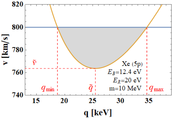
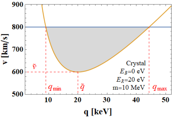
Figure 1: Function $v_{\rm min}(q,E_{\rm R}+E_{\rm B})$ in Eq. (23) (orange line) and integration range in $q$ in Eq. (40) for $m=10$ MeV, $E_{\rm R}=20$ eV, and the 5p orbital in a xenon target with $E_{\rm B}=12.4$ eV (left panel) and for a semiconductor target thus $E_{\rm R}=E_{e}$ (right panel). We call generically $E_{\rm R}$ the detectable energy in both cases. Shown here are $\tilde{v}$ (the minimum $v_{\rm min}$ value), $\tilde{q}=q_{\pm}(\tilde{v})$, $q_{\rm min}=q_{-}(v_{\rm max},E_{\rm R}+E_{\rm B})$ and $q_{\rm max}=q_{+}(v_{\rm max},E_{\rm R}+E_{\rm B})$. Here $v_{\rm max}=$ 800 km/s, corresponding to DM bound to the Galaxy.

The function $v_{\rm min}(q,E_{e})$ in Eq. (23) is shown in Fig. 1 as function of $q$ (orange lines) for $m=10$ MeV, $E_{\rm R}=20$ eV and either $E_{\rm B}=12.4$ eV (left panel), corresponding to the 5p orbital of a Xe atom, or $E_{\rm B}=0$ (right panel), corresponding to electrons jumping between two bands of a semiconductor crystal, where the whole energy change is observable.

For fixed $E_{e}$, $q$ as function of $v_{\rm min}$ has two solutions,

$$q_{\pm}(v_{\rm min},E_{e})=mv_{\rm min}\left(1\pm\sqrt{1-\frac{2E_{e}}{mv_{\rm min}^{2}}}\right)~{},$$ (25)

which meet at the minimum $v_{\rm min}$ value

$$\tilde{v}=\sqrt{2E_{e}/m}~{},$$ (26)

where $q$ has the value

$$q_{\pm}(\tilde{v},E_{e})=\tilde{q}=\sqrt{2mE_{e}}~{},$$ (27)

as shown in Fig. 1.

The maximum possible value of $v_{\rm min}$ is the maximum possible speed $v_{\rm max}$ of a DM particle in Earth’s frame. The maximum speed of a DM particle bound to the halo of the Galaxy is the escape speed from the Galaxy at the position of the Solar System ($\simeq 550$ km/s Piffl:2013mla ; Monari:2018 ; Deason:2019 ) plus the speed of the Sun with respect to the Galaxy ($\simeq 240$ km/s, see Benito:2019ngh for discussion of uncertainties), which we take to be $v_{\rm max}=$ 800 km/s. DM that is not bound to the Galaxy, such as DM from the Local Group and the Virgo Cluster, could in principle also contribute subdominantly to direct detection Baushev:2012dm ; Freese:2001hk ; Herrera:2021puj , in which case $v_{\rm max}$ would be larger. We do not consider this possibility, but our formalism can readily accommodate it, by changing the value of $v_{\rm max}$.

The maximum and minimum values of $q$ for a given $E_{e}$ (also shown in Fig. 1) are thus

$$q_{\rm min}=q_{-}(v_{\rm max},E_{e})~{},~{}~{}~{}~{}~{}q_{\rm max}=q_{+}(v_{\rm max},E_{e})~{}.$$ (28)

Using the general formulas for DM-induced electronic transitions in App. A of Ref. Essig:2015cda (and references there in) we take the cross section for the transition of a given target electron from an initial state $i$ to a final state $f$ to be

$$\sigma v_{i\to f}=\frac{\overline{\sigma}_{e}}{\mu_{\chi e}^{2}}\int\frac{d^{3}q}{4\pi}\,\delta\Big{(}\Delta E_{i\to f}+\frac{q^{2}}{2m}-qv\cos\theta_{qv}\Big{)}\times|F_{\rm DM}(q)|^{2}|f_{i\to f}(\vec{q}\,)|^{2}~{}.$$ (29)

Here the reference cross section $\sigma_{\rm ref}=\overline{\sigma}_{e}$ is the non-relativistic DM–electron elastic scattering cross section with the momentum transfer $q$ fixed to the reference value $\alpha m_{e}$ (the characteristic speed of a bound atomic electron is the fine structure constant $\alpha$), $\mu_{\chi e}$ is the DM-electron reduced mass, $|f_{i\rightarrow f}(\vec{q})|$ is the electron form factor, $F_{\rm DM}(q)$ is a DM form factor that we take to be either $1$ or $(\alpha~{}m_{e}/q)^{2}$. The time-average rate for this transition, obtained with the time average DM velocity distribution $f_{\chi}(\vec{v})$ is

$$R_{i\to f}=\frac{\rho}{m}\int d^{3}v\,f_{\chi}(\vec{v})\,\sigma v_{i\to f}~{}.$$ (30)

We show in App. A that summing these transition rates over all initial and final electron states, while including the factor

$$1=\int\text{d}E_{\rm R}~{}\delta(E_{\rm R}-\Delta E_{i\to f}+E_{{\rm B}i})$$ (31)

in the integration to insure that the detectable energy has a fixed value $E_{\rm R}$, we obtain the differential event rate (see Eq. (69)),

$$\frac{\text{d}R}{\text{d}E_{\rm R}}=\frac{1}{2\mu^{2}_{\chi e}}\frac{1}{E_{\rm R}}\sideset{}{{}^{\prime}}{\sum}_{i,f}\int_{q_{\rm min}}^{q_{\rm max}}\text{d}q\,q~{}\tilde{\eta}(v_{\rm min}(q,E_{\rm R}+E_{{\rm B}i}))~{}|F_{\rm DM}(q)|^{2}|f^{i,f}(q,E_{\rm R})|^{2}.$$ (32)

Here $\tilde{\eta}(v_{\rm min}(q,E_{\rm R}+E_{{\rm B}i}))$ is the time-average of the function defined in Eq. (1) (see Eq. (2)) with $\sigma_{\rm ref}=\overline{\sigma}_{e}$, the symbol $\sideset{}{{}^{\prime}}{\sum}_{i,f}$ indicates the sum over distinct initial and final energies, and we have defined the electron form factor

$$|f^{i,f}(q,E_{\rm R})|^{2}=\sum_{\begin{subarray}{c}\rm degen.\\ \rm states\end{subarray}}E_{\rm R}~{}\delta(E_{\rm R}-\Delta E_{i\rightarrow f}+E_{{\rm B}i})|f_{i\rightarrow f}(\vec{q})|^{2}.$$ (33)

After performing the summations over all degenerate states, which include summing over all directions, the electron form factor $|f^{i,f}(q,E_{\rm R})|$ is independent of the direction of $\vec{q}$ (as pointed out in Ref. Essig:2015cda ).

Here $E_{{\rm B}i}$ is non-zero only when the electron is bound in the initial state and free in the final state (it is the binding energy of the initial state) and should be taken to be zero $E_{{\rm B}i}=0$ otherwise (recall that in a crystal $\Delta E_{i\to f}$ is the detectable energy, which to use a common notation we still call $E_{\rm R}$),

To bring the rate in Eq. (32) into the form in Eq. (15) and thus identify the response function, we chose $v_{\rm min}$ as the independent variable instead of $q$ and change the integration variable using $\text{d}q_{\pm}=J_{\pm}(v_{\rm min},E_{\rm R}+E_{{\rm B}i})~{}\text{d}v_{\rm min}$, with the Jacobian factors

$$J_{\pm}(v_{\rm min},E_{\rm R}+E_{{\rm B}i}) = \frac{\partial q_{\pm}(v_{\rm min},E_{\rm B}+E_{\rm R})}{\partial v_{\rm min}}$$ (34)

$$= m\left(1\pm\dfrac{1}{\sqrt{1-\dfrac{(E_{\rm R}+E_{{\rm B}i})}{m~{}v_{\rm min}^{2}/2}}}\right)=m\left(1\pm\dfrac{1}{\sqrt{1-\dfrac{\tilde{v}^{2}}{v_{\rm min}^{2}}}}\right).$$

Calling $I(q,v_{\rm min},E_{\rm R})$ the integrand, the integral in $q$ in Eq. (32) becomes

$$\int_{q_{\rm min}}^{q_{\rm max}}dq\,I(q,v_{\rm min}(q,E_{\rm R}+E_{{\rm B}i}),E_{\rm R})$$ (35)

$$= \int_{q_{\rm min}}^{q_{0}}dq\,I(q,v_{\rm min}(q,E_{\rm R}+E_{{\rm B}i}),E_{\rm R})+\int_{q_{0}}^{q_{\rm max}}dq\,I(q,v_{\rm min}(q,E_{\rm R}+E_{{\rm B}i}),E_{\rm R})$$

$$= \int^{v_{\rm max}}_{\tilde{v}}dv_{\rm min}\,(J_{+}-J_{-})~{}I(q(v_{\rm min},E_{\rm R}+E_{{\rm B}i}),v_{\rm min},E_{\rm R})\,.$$

Here $v_{\rm max}$ is the maximum value of $v_{\rm min}$ and the negative sign in front of $J_{-}$ is due to the change of integration order because $q_{\rm min}=q(v_{\rm max})$.

Notice that for any fixed value of $E_{\rm R}$ the two Jacobian factors $J_{+}$ and $J_{-}$ in Eq. (34) diverge at $v_{\rm min}=\tilde{v}=\sqrt{2E_{e}/m}$. This would then mean that the window function in $v_{\rm min}$ for each $E_{{\rm B}i}+E_{\rm R}$ energy diverges at $\tilde{v}$, so that the rate measured at a particular $E_{\rm R}$ would give information on the $\tilde{\eta}$ function only at the particular $\tilde{v}$ value. However, as we explain below, we will integrate over $E_{R}$, and as function of $E_{R}$ the integral of the Jacobian factors is finite, because it is of the form $\int dx/x^{1/2}$. Thus the result of any integration in $E_{\rm R}$ of the Jacobian multiplied by any non-singular function of $E_{\rm R}$ is finite (since it is always smaller than the integral of the Jacobian multiplied by the maximum value of the function in the integration range). We do need to integrate over $E_{\rm R}$ even for unbinned data, because the measured energy $E^{\prime}$ of an event always corresponds to a range of $E_{\rm R}$ given by the experimental energy resolution function. In fact, the observable differential spectrum (as mentioned earlier, see Eq. (8))

$$\frac{\text{d}R}{\text{d}E^{\prime}}=\epsilon(E^{\prime})\int_{0}^{E_{\rm max}}\text{d}E_{\rm R}\,G(E^{\prime},E_{\rm R})\frac{\text{d}R}{\text{d}E_{\rm R}}~{},$$ (36)

depends on the energy resolution function $G(E^{\prime},E_{\rm R})$ (and also on the counting efficiency $\epsilon(E^{\prime})$).

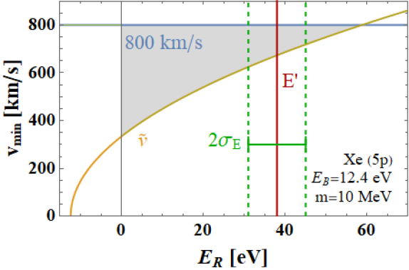
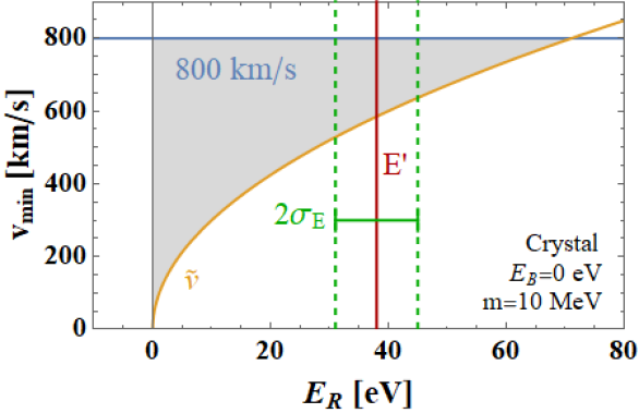
Figure 2: Integration domain (in gray) in $(E_{\rm R},v_{\rm min})$ space in Eq. (36) and Eq. (39) for $E^{\prime}=38$ eV and a box energy resolution function $G(E^{\prime},E_{\rm R})$ with width $2\sigma_{\rm E}=14$ eV centered at $E^{\prime}$, for the 5p orbital of a Xe atom, $E_{\rm B}=12.4$ eV (left panel) and for a semiconductor target, $E_{\rm B}=0$ (right panel). Green dashed vertical lines indicate the range in which the energy resolution function $G(E^{\prime},E_{\rm R})$ is non-zero. The integration range in $E_{\rm R}$ goes between $E^{\prime}-\sigma_{\rm E}$ and $E^{\prime}+\sigma_{\rm E}$ or between $E^{\prime}-\sigma_{\rm E}$ and the orange line $E_{\rm R}(\tilde{v})$ when $E_{\rm R}(\tilde{v})<E^{\prime}+\sigma_{\rm E}$.

We can now write the time-averaged differential rate into the form in Eq. (15),

$$\frac{\text{d}R}{\text{d}E^{\prime}}=\int^{v_{\rm max}}_{\tilde{v}}\text{d}{v_{\rm min}}~{}\frac{\text{d}\mathcal{R}}{\text{d}E^{\prime}}(v_{\rm min},E^{\prime})~{}\tilde{\eta}(v_{\rm min})~{},$$ (37)

namely as a convolution of the time-averaged $\tilde{\eta}(v_{\rm min})$ in Eq. (2) and the response function, which we identify to be

$$\frac{\text{d}\mathcal{R}}{\text{d}E^{\prime}}(v_{\rm min},E^{\prime})=\left(\frac{\text{d}\mathcal{R}^{+}}{\text{d}E^{\prime}}-\frac{\text{d}\mathcal{R}^{-}}{\text{d}E^{\prime}}\right)~{},$$ (38)

where

$$\frac{d\mathcal{R}_{\pm}}{dE^{\prime}}(v_{\rm min},E^{\prime}) = \frac{\epsilon(E^{\prime})}{2\mu^{2}_{\chi e}}\sideset{}{{}^{\prime}}{\sum}_{i,f}\int_{0}^{E_{\rm max}}\frac{dE_{\rm R}}{E_{\rm R}}G(E^{\prime},E_{\rm R})J_{\pm}(v_{\rm min},E_{\rm R}+E_{{\rm B}i})~{}q_{\pm}(v_{\rm min},E_{\rm R}+E_{{\rm B}i})$$ (39)

$$|F_{\rm DM}(q_{\pm}(v_{\rm min},E_{\rm R}+E_{{\rm B}i}))|^{2}|f^{i,f}(q_{\pm}(v_{\rm min},E_{\rm R}+E_{{\rm B}i}),E_{\rm R})|^{2}~{}.$$

Here, $E_{\rm max}=\frac{1}{2}mv_{\rm min}^{2}-E_{{\rm B}i}$. The boundaries of the integration domain in the $(E_{\rm R},v_{\rm min})$ plane, are easily determined and shown in Fig. 2. In the $(q,v_{\rm min})$ plane, the integration domain is bounded from below by the function $v_{\rm min}(q,E_{\rm R}+E_{\rm B})$ in Eq. (23), and from above by the maximum $v_{\rm min}$ value, $v_{\rm max}$. For any $E_{\rm R}>0$, there is only one minimum of $v_{\rm min}$, $\tilde{v}$, corresponding to $q=\tilde{q}$. The DM particle speed has to be greater than $\tilde{v}$ to be detectable. Therefore, in the $(E_{\rm R},v_{\rm min})$ plane, for positive $E_{\rm R}$, the integration domain is bounded by the maximum and minimum $v_{\rm min}$ values, as shown in Fig. 2. For each fixed $v_{\rm min}$ value in the range $\sqrt{2E_{{\rm B}i}/m}\leq v_{\rm min}\leq v_{\rm max}$, the $E_{\rm R}$ integration range is $0\leq E_{\rm R}\leq E_{\rm max}=\frac{1}{2}mv_{\rm min}^{2}-E_{{\rm B}i}$.

Any experimental energy resolution $G(E^{\prime},E_{\rm R})$ has a finite width $\sigma_{\rm E}$. We show in Fig. 3 how the shape of the response function’s peak (normalized by its maximum value so as to always place the maximum of the ratio close to 1) changes as $\sigma_{\rm E}$ increases, for a box resolution function $G(E^{\prime},E_{\rm R})$ of width $2~{}\sigma_{\rm E}$ centered at $E^{\prime}$, $m=$10 MeV and $E^{\prime}=$ 15 eV, and for simplicity the electron form factor set to 1, $|f^{i,f}|=1$. Fig. 3 demonstrates that the response function would have a sharp peak as $\sigma_{\rm E}\to 0$, which progressively disappears as $\sigma_{\rm E}$ increases.

An alternative derivation of the response function in Eqs.(38) and (39) based on computing first the response function $\text{d}\mathcal{H}(E^{\prime},v)/\text{d}E^{\prime}$ for the DM speed distribution, so that the rate is given by Eq. (9), and then using the relation in Eq. (12) to compute $\text{d}\mathcal{R}(E^{\prime},v)/\text{d}E^{\prime}$ as its derivative with respect to the speed $v$ is presented in App. E. The function $\text{d}\mathcal{H}(E^{\prime},v)/\text{d}E^{\prime}$ is given in Eq. (100). It is regular for all values of the energy and depends on the speed $v$ only though the limits of the integration in $q$. Taking the partial derivative of this function with respect to $v$, and recalling that we defined in Eq. (34) ${\partial q_{\pm}(v,E_{e})}/{\partial v}=J_{\pm}(v,E_{e})$, we recover Eq. (38) and Eq. (39).

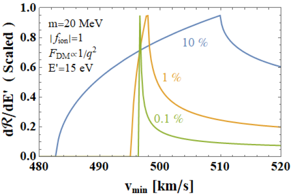
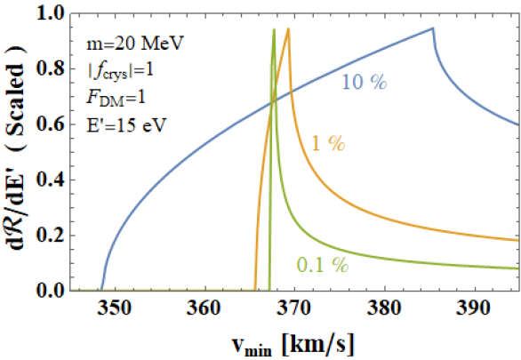
Figure 3: Dependence on the width $\sigma_{\rm E}$ of the energy resolution function of the response function $\text{d}\mathcal{R}/\text{d}E^{\prime}$ near $v_{\rm min}=\tilde{v}$ where the Jacobian $J_{\pm}(v_{\rm min},E_{\rm B}+E_{\rm R})$ in Eq.(34) has a singularity, assuming a box resolution function as in Eq. (51), with $\sigma_{E}$ equal to 0.1%, 1% and 10% of $E^{\prime}$, for $m$=20 MeV, $E^{\prime}$=15 eV and electron form factor set to 1. It shows that a realistic non-zero experimental $\sigma_{\rm E}$ can effectively smooth out the peak.

3.1 Atomic ionization due to DM scattering

The DM particle can scatter with a bound electron in a particular orbital of an atom ionizing it by taking the electron to an unbound state $E_{\rm R}=k^{2}/2m_{e}$. In an atom target, the initial bound states are labeled by the principal quantum number $n$ and the angular momentum quantum number $l$, $|i\rangle=|nl\rangle$, and the final states are free spherical wave states. The rate given in Refs. Essig:2011nj ; Essig:2012yx ; Essig:2017kqs ; Emken:2019tni is

$$\frac{dR_{\rm ion}}{dE_{\rm R}}=\sum_{nl}\frac{1}{8\mu_{\chi e}^{2}}\frac{1}{E_{\rm R}}\int_{q_{\rm min}}^{q_{\rm max}}\text{d}q\,q~{}\tilde{\eta}(v_{\rm min}(q,E_{\rm R}+E_{Bnl}))~{}|F_{\rm DM}(q)|^{2}~{}|f^{nl}_{\rm ion}(q,E_{\rm R})|^{2}~{},$$ (40)

where the limits of integration $q_{\rm min}$ and $q_{\rm max}$ are given in Eq. (28). Notice that this coincides with the general rate in Eq. (32) by identifying the electron form factors,

$$\sideset{}{{}^{\prime}}{\sum}_{i,f}|f^{i,f}(q,E_{\rm R})|^{2}=\dfrac{1}{4}\sum_{nl}|f^{nl}_{\rm ion}(q,E_{\rm R})|^{2}~{}.$$ (41)

This identification is done more precisely in App. B, using the definition of the form factor $\sum_{nl}|f^{nl}_{\rm ion}(q,E_{\rm R})|^{2}$ given in Eq.(6) of Ref. Essig:2011nj (see Eq. (74)).

Given the experimental energy resolution function of a particular xenon based detector, $G_{\rm ion}(E^{\prime},E_{\rm R})$, the observable DM ionization rate becomes

$$\frac{\text{d}R_{\rm ion}}{\text{d}E^{\prime}}=\int^{v_{max}}_{\tilde{v}}\text{d}v_{\rm min}~{}\frac{\text{d}\mathcal{R}_{\rm ion}}{\text{d}E^{\prime}}(v_{\rm min},E^{\prime})~{}\tilde{\eta}(v_{\rm min}),$$ (42)

where the response function is

$$\frac{\text{d}\mathcal{R}_{\rm ion}}{\text{d}E^{\prime}}=\frac{\text{d}\mathcal{R}_{\rm ion}^{+}}{\text{d}E^{\prime}}-\frac{\text{d}\mathcal{R}_{\rm ion}^{-}}{\text{d}E^{\prime}}$$ (43)

with

$$\frac{\text{d}\mathcal{R}^{\pm}_{\rm ion}}{\text{d}E^{\prime}}(v_{\rm min},E^{\prime}) = \frac{\epsilon(E^{\prime})}{8\mu^{2}_{\chi e}}\sum_{nl}\int\frac{\text{d}E_{\rm R}}{E_{\rm R}}\,G_{\rm ion}(E^{\prime},E_{\rm R})~{}J_{\pm}(v_{\rm min},E_{\rm R}+E_{{\rm B}nl})q_{\pm}(v_{\rm min},E_{\rm R}+E_{{\rm B}nl})$$ (44)

$$\times|F_{\rm DM}(q_{\pm}(v_{\rm min},E_{\rm R}+E_{{\rm B}nl}))|^{2}|f^{nl}_{\rm ion}(q_{\pm}(v_{\rm min},E_{\rm R}+E_{{\rm B}nl}),E_{\rm R})|^{2}~{}.$$

Here, the electron form factors $|f^{nl}_{\rm ion}|^{2}$ are those computed in Ref. Essig:2015cda that we use in our numerical calculations, as explained below in Sec. 3.3. In Fig 4 we show the contribution to the response function of xenon atoms of several initial state orbitals, ${\text{d}\mathcal{R}^{nl}_{\rm ion}}/{\text{d}E^{\prime}}$, which we defined so that

$$\frac{\text{d}\mathcal{R}_{\rm ion}}{\text{d}E^{\prime}}=\sum_{nl}\frac{\text{d}\mathcal{R}^{nl}_{\rm ion}}{\text{d}E^{\prime}}~{}.$$ (45)

In our numerical calculations (explained in Sec. 3.3), we will only use the 4d and 5p orbitals since they provide the dominant contributions to the response function in xenon.

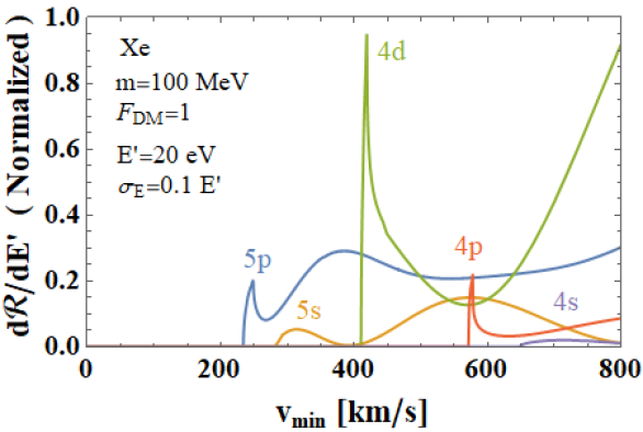
Figure 4: Contribution of several initial state orbitals to the ionization response function ${\text{d}\mathcal{R}_{\rm ion}}/{\text{d}E^{\prime}}$ in xenon (see Eqs. (42) to (45)), for DM mass $m=100$ MeV, $E^{\prime}=20$ eV and a box energy resolution function with $\sigma_{\rm E}=0.10E^{\prime}$. In our numerical calculations we only include the dominant 5p and 4d contributions.

3.2 DM scattering in semiconductor crystals

In this case, upon scattering, an electron in the valence band can be excited to a conduction band of the crystal. Since the band gap energy is significantly smaller than the binding energy of orbital electrons, (it is about 1 eV instead of the about 10 eV of ionization threshold in xenon) crystals have lower threshold and thus greater potential for detecting DM with smaller kinetic energy. The differential rate given in Refs. Essig:2015cda ; Emken:2019tni in this case is

$$\frac{dR_{\rm crys}}{dE_{\rm R}}=N_{\rm cell}\frac{\alpha m_{e}^{2}}{\mu_{\chi e}^{2}}\int dq\,\frac{1}{q^{2}}\tilde{\eta}(v_{\rm min}(q,E_{\rm R}))~{}|F_{\rm DM}(q,E_{\rm R})|^{2}~{}|f_{\rm crys}(q,E_{\rm R})|^{2}|~{},$$ (46)

where $N_{\rm cell}$ is number of unit cells in the crystal.

Notice that Eq. (46) coincides with the general rate in Eq. (32) by taking $E_{{\rm B}i}=0$ and identifying the electron form factor as

$$\sideset{}{{}^{\prime}}{\sum}_{i,f}|f^{i,f}(q,E_{\rm R})|^{2}=\dfrac{2\alpha m_{e}^{2}~{}N_{\rm cell}}{q^{3}}~{}|f_{\rm crys}(q,E_{\rm R})|^{2}~{}.$$ (47)

This identification is done more precisely in App. C, using the definition of the electron form factor $|f_{\rm crys}(q,E_{\rm R})|^{2}$ in a semiconductor crystal in Eq. (A.33) of Ref. Essig:2015cda (see Eq. (87)).

The rate can now be written as

$$\frac{\text{d}R_{\rm crys}}{\text{d}E^{\prime}}=\int^{v_{\rm max}}_{0}\text{d}v_{\rm min}~{}\frac{\text{d}\mathcal{R}_{\rm crys}}{\text{d}E^{\prime}}(v_{\rm min},E^{\prime})~{}\tilde{\eta}(v_{\rm min})~{}.$$ (48)

with the crystal response function

$$\frac{\text{d}\mathcal{R}_{\rm crys}}{\text{d}E^{\prime}}(v_{\rm min},E^{\prime})=\frac{\text{d}\mathcal{R}_{\rm crys}^{+}}{\text{d}E^{\prime}}-\frac{\text{d}\mathcal{R}_{\rm crys}^{-}}{\text{d}E^{\prime}}~{},$$ (49)

where

$$\frac{\text{d}\mathcal{R}_{\rm crys}^{\pm}}{\text{d}E^{\prime}}(v_{\rm min},E^{\prime}) = \frac{N_{\rm cell}\epsilon(E^{\prime})}{\mu^{2}_{\chi e}}(\alpha m_{e}^{2})\int_{0}^{E_{\rm max}}\text{d}E_{\rm R}\,G_{\rm crys}(E^{\prime},E_{\rm R})\dfrac{J_{\pm}(v_{\rm min},E_{\rm R})}{q_{\pm}^{2}(v_{\rm min},E_{\rm R})}$$ (50)

$$\times|F_{\rm DM}(q_{\pm}(v_{\rm min},E_{\rm R}))|^{2}~{}|f_{\rm crys}(q_{\pm}(v_{\rm min},E_{\rm R}),E_{\rm R})|^{2}.$$

Again, in this case the electron form factors are those computed in Ref. Essig:2015cda that we use in our numerical calculations, as explained below.

3.3 Numerical evaluations of response functions

We now describe a general procedure for numerically evaluating the response functions using already provided electron form factor $|f^{i,f}(q,E_{\rm R})|^{2}$ data in energy bins of width $\Delta E_{\rm R}$ and momentum transfer bins of width $\Delta q$. The integrals we need to compute in Eq. (44) for xenon and in Eq. (50) for semiconductor crystals, are discretized into partitions small enough for the electron form factor in each to be taken as a constant, and the remaining integral is calculated analytically. All the relevant information about the target material electronic structure is contained within the dimensionless form factor that is independent of any physics related to DM. For the crystal form factor $|f_{\rm crys}|^{2}$ we employ the output data from the QEdark Essig:2015cda , a module for Quantum Espresso Giannozzi:2009 based on density functional theory. For the xenon form factor $|f_{\rm ion}|^{2}$ we use the data output from Ref. Essig:2015cda , in which electronic wave functions are computed assuming a spherical atomic potential and filled electron shells.

To compute the response function in Eq. (39) (specifically to compute the functions in Eq. (44) and Eq. (50)), we need to specify the energy resolution function, the DM form factor, and electron form factors. For simplicity, we assume a simple box function for the energy resolution,

$$G(E^{\prime},E)=\dfrac{1}{2\sigma_{\rm E}}\textrm{UnitBox}\Big{[}\dfrac{E_{\rm R}-E^{\prime}}{2\sigma_{\rm E}}\Big{]}~{}.$$ (51)

With a more realistic Gaussian distribution, the results are very similar. As can be seen from Eq. (39), the resolution width $\sigma_{\rm E}$ affects the limits of integration in energy, thus summation range when the energy range is discretized to perform numerical evaluations. Fig. 3 shows how the value of $\sigma_{\rm E}$ affects the form of the response function close to the singularity point of the Jacobian. For the other figures we assumed the resolution $\sigma_{\rm E}=0.10E^{\prime}$.

As already mentioned, following Ref. Essig:2015cda we consider two DM form factors, $F_{\rm DM}(q)=1$ or $F_{\rm DM}(q)=({\alpha m_{e}}/{q})^{2}$, which generically appear in a variety of models such as scenarios of vector-portal DM with a dark photon mediator or magnetic-dipole-moment interactions.

We discretize the $(E_{\rm R},q)$ plane into a mesh of partitions labelled by $(E_{s},q_{r})$. The form factor can then be written as $q_{\pm}^{a}E_{\rm R}^{b}|f^{i,f}_{\rm dat}|^{2}_{rs}$, where $|f^{i,f}_{\rm dat}|^{2}_{rs}$ is a given data entry. For crystals, the data is already provided in bins. For atoms, the table provided was interpolated to find the value at the lowest $q$, $E$ in each partition (and assign it to the partition). Hence, the function in the $(E_{\rm R},q)$ plane can be written as a matrix $|f_{\rm dat}|^{2}_{rs}$, as shown in Fig. 5.

To perform the integration for the response function numerically, our procedure is the following. Since we are integrating over the path in the $(E_{\rm R},q)$ plane described by the function $q(v_{\rm min},E_{\rm R})$ at a given $v_{\rm min}$, we only need to count the binned partitions that the function passes through. As illustrated on Fig. 5, for some given form factor data (e.g. semiconductor crystals  Essig:2015cda ), for each $\Delta E$ bin more than one $\Delta q$ bin might need to be considered. Hence, we use the average value of the electron form factor, weighted by the area of the shaded region in each $q$ interval shown in Fig. 5. This involves finding the $E_{\rm R}$ value at the intersection of the path taken by $q(v_{\rm min},E_{\rm R})$ with each of the $q$ partition boundaries, which is done via Eq. (23) for a fixed $v_{\rm min}$. The resulting $E_{\rm R}$ points divide $\Delta E$ into smaller sub-intervals, for which we use the corresponding $|f_{\rm dat}|^{2}_{rs}$ values. Finally, we sum over all possible energy bins within the given $(E^{\prime}-\sigma_{\rm E},E_{\rm max})$ range.

Extracting the electron form factor data value $|f^{i,f}_{\rm data}(E_{\rm R},q_{\pm})|^{2}$ in each $(E_{1}^{(rs)},E_{2}^{(rs)})$ bin from the definition of the response function in Eq. (39), we compute analytically the remaining integral, i.e. we write the response function for each bin as

$$\frac{d\mathcal{R}_{\pm}}{dE^{\prime}} (v_{\rm min},E_{1}^{(rs)},E_{2}^{(rs)})=\frac{\epsilon(E^{\prime})}{2\mu^{2}_{\chi e}}|f^{i,f}_{\rm dat}(E_{1}^{(rs)},q_{\pm})|^{2}\int_{E_{1}^{(rs)}}^{E_{2}^{(rs)}}\frac{dE_{\rm R}}{E_{\rm R}}~{}q_{\pm}^{a}E_{\rm R}^{b}~{}G(E^{\prime},E_{\rm R})$$ (52)

$$\times|J_{\pm}(v_{\rm min},E_{\rm R}+E_{{\rm B}i})q_{\pm}(v_{\rm min},E_{\rm R}+E_{{\rm B}i})|F_{\rm DM}(q_{\pm}(v_{\rm min},E_{\rm R}+E_{{\rm B}i}))|^{2}.$$

Notice the $q_{\pm}^{a}E_{\rm R}^{b}$ factor, stemming from the fact that the electron form factor in terms of the data values provided in Ref. Essig:2015cda is $|f^{i,f}(q_{\pm},E_{\rm R})|^{2}=q_{\pm}^{a}E_{\rm R}^{b}|f^{i,f}_{\rm data}(E_{\rm R},q_{\pm})|^{2}$, where $a=b=0$ for atoms and $a=-3$ and $b=1$ for crystals. Then, writing $|F_{\rm DM}(q)|^{2}=(\alpha m_{e})^{2c}q^{-2c}$, with either $c=0$ or $c=2$, we evaluate the entire response function. The expression for the response function in terms of the $a$, $b$ and $c$ constants is given in the App. D (see Eq. (90) of App. D).

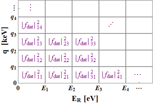
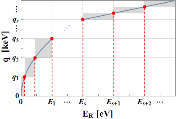
Figure 5: Discretization mesh of the electron form factor data $|f_{\rm dat}|^{2}_{rs}$ (left panel) and an example of response function integration path $q(v_{\rm min},E_{\rm R})$ for fixed $v_{\rm min}$, in the $(E_{\rm R},q)$ plane.

For atoms (corresponding to $a=b=0$ in Eq. (91)), the response function is

$$\frac{\text{d}\mathcal{R}^{\pm}_{\rm ion}}{\text{d}E^{\prime}}(v_{\rm min},E^{\prime})=\frac{\epsilon(E^{\prime})}{16\mu_{\chi e}^{2}\sigma_{\rm E}}(\alpha m_{e})^{2c}\sum_{nl}\sum_{{\rm Path}(r,s)}I^{\pm,nl}_{\rm ion}(v_{\rm min},E_{1}^{(rs)},E_{2}^{(rs)})|f_{\rm ion}^{nl}|^{2}_{rs}~{}.$$ (53)

Here, the summation is over all the $(r,s)$ partitions along the path in the $(E_{\rm R},q)$ plane of the function $q(v_{\rm min},E_{\rm R})$ for fixed $v_{\rm min}$, as indicated in Fig. 5, and

$$I_{\rm ion}^{\pm,nl}(v_{\rm min},E_{1}^{(rs)},E_{2}^{(rs)})\simeq\int_{E_{1}^{(rs)}}^{E_{2}^{(rs)}}\text{d}E_{\rm R}\,\frac{q_{\pm}^{1-2c}(v_{\rm min},E_{\rm R}+E_{{\rm B}nl})\,J_{\pm}(v_{\rm min},E_{\rm R}+E_{{\rm B}nl})}{(E_{1}^{(rs)}+E_{2}^{(rs)})/2}.$$ (54)

Thus,

$$I_{\rm ion}^{\pm,nl}(v_{\rm min},E_{1}^{(rs)},E_{2}^{(rs)})\simeq\begin{cases}\dfrac{\mp(mv_{\rm min})^{3}}{3(E_{1}^{(rs)}+E_{2}^{(rs)})}\left.\left[\left(1\pm\sqrt{1-\dfrac{2(E_{\rm R}+E_{{\rm B}nl})}{mv_{\rm min}^{2}}}\right)^{3}\right]\right|_{E_{1}^{(rs)}}^{E_{2}^{(rs)}}~{},&{\rm if}~{}c=0;\\ \\ \dfrac{\pm(mv_{\rm min})^{-1}}{(E_{1}^{(rs)}+E_{2}^{(rs)})}\left.\left[\left(1\pm\sqrt{1-\dfrac{2(E_{\rm R}+E_{{\rm B}nl})}{mv_{\rm min}^{2}}}\right)^{-1}\right]\right|_{E_{1}^{(rs)}}^{E_{2}^{(rs)}}~{},&{\rm if}~{}c=2~{}.\end{cases}$$ (55)

For semiconductor targets (corresponding to $a=-3$ and $b=1$ in Eq. (91)), the response function is

$$\frac{\text{d}\mathcal{R}_{\rm crys}^{\pm}}{\text{d}E^{\prime}}(v_{\rm min},E^{\prime})=\frac{\epsilon(E^{\prime})N_{\rm cell}(\alpha m_{e}^{2})}{2\mu_{\chi e}^{2}\sigma_{\rm E}}(\alpha m_{e})^{2c}\sum_{{\rm Path}(r,s)}I^{\pm}_{\rm crys}(v_{\rm min},E_{1}^{(rs)},E_{2}^{(rs)})|f_{\rm crys}|^{2}_{rs},$$ (56)

where,

$$I_{\rm crys}^{\pm}(v_{\rm min},E_{1}^{(rs)},E_{2}^{(rs)}) \simeq \int_{E_{1}^{(rs)}}^{E_{2}^{(rs)}}\text{d}E_{\rm R}\,q_{\pm}^{-2-2c}(v_{\rm min},E_{\rm R})J_{\pm}(v_{\rm min},E_{\rm R})$$ (57)

$$= \begin{cases}\mp\left.\left[\ln\left|1\pm\sqrt{1-\dfrac{2E_{\rm R}}{mv_{\rm min}^{2}}}\right|\right]\right|_{E_{1}^{(rs)}}^{E_{2}^{(rs)}}~{},&{\rm if}~{}c=0~{};\\ \\ \dfrac{\pm 1}{4(mv_{\rm min})^{4}}\left.\left[\left(1\pm\sqrt{1-\dfrac{2E_{\rm R}}{mv_{\rm min}^{2}}}\right)^{-4}\right]\right|_{E_{1}^{(rs)}}^{E_{2}^{(rs)}}~{},&{\rm if}~{}c=2~{}.\end{cases}$$

In our numerical evaluations, for Si and Ge crystals we use the QEdark Essig:2015cda output data for the computed electron form factors, given in the 0 to 50 eV energy range and 0 to $18~{}\alpha m_{e}$ momentum range with $\Delta E_{\rm R}=0.1$ eV and $\Delta q=0.02\,\alpha m_{e}$. For Xe atoms, we use the same binning and the data table provided in Ref. Essig:2015cda for the electron form factors in the 0.2 to 900 eV energy range and the $0.37~{}\alpha m_{e}=1.4$ keV to $54.60~{}\alpha m_{e}=203.7$ keV momentum range. The maximum of this range is smaller than $q_{\rm max}=q_{+}(800{\rm km/s})$ except for the lightest DM masses we consider. The table was interpolated to find the form factor value at the lowest $E_{\rm R}$ and $q$ point in each bin, which was assigned to the bin.

The response functions depend on the DM particle mass $m$, the detected energy $E^{\prime}$, and the minimum speed $v_{\rm min}$. For our figures we chose a set of values for energies $E^{\prime}=$ 15 eV, 30 eV and 45 eV and additionally $E^{\prime}=$ 5 eV for semiconductors (in Xe, the minimum detectable energy is 13.8 eV) and DM masses $m=$ 20 MeV, 100 MeV, 1 GeV that are within the reach of current and near-future experiments, including Ge-based EDELWEISS Armengaud:2018cuy ; Armengaud:2019kfj ; Arnaud:2020svb , SuperCDMS and Si-based DAMIC deMelloNeto:2015mca ; Aguilar-Arevalo:2019wdi ; Settimo:2020cbq , SENSEI Tiffenberg:2017aac ; Crisler:2018gci ; Abramoff:2019dfb ; Barak:2020fql , SuperCDMS Agnese:2014aze ; Agnese:2015nto ; Agnese:2016cpb ; Agnese:2017jvy ; Agnese:2018col ; Agnese:2018gze ; Amaral:2020ryn and Xe-based Essig:2011nj ; Graham:2012su ; Lee:2015qva ; Essig:2017kqs ; Catena:2019gfa ; Agnes:2018oej ; Aprile:2019xxb ; Aprile:2020tmw experiments.

3.4 Inelastic DM electron scattering and other possibilities

In the case of inelastic electron-DM scattering the DM is multi-component and the initial DM particle of mass $m$ scatters into another of mass $m^{\prime}$. The mass difference is $\delta=m^{\prime}-m\ll m\simeq m^{\prime}$. Going through the same steps we followed in Sec. 3, from the kinematics of the collision we obtain

$$v_{\rm min}=\dfrac{E_{\rm R}+E_{\rm B}}{q}\Big{(}1+\dfrac{\delta}{m}\Big{)}+\dfrac{q}{m}=\Big{(}\dfrac{E_{\rm R}+E_{\rm B}}{q}+\dfrac{q}{2m^{\prime}}\Big{)}\Big{(}1+\dfrac{\delta}{m^{\prime}}\Big{)}~{}.$$ (58)

Hence, our halo-independent DM-electron elastic scattering analysis can be readily adapted to inelastic scattering by either scaling $(E_{\rm R}+E_{\rm B})$ to $(E_{\rm R}+E_{\rm B})(1+\delta/m_{1})$ for the same $v_{\rm min}$ or, alternatively, scaling the speed $v_{\rm min}$ to $v_{\rm min}/(1+\delta/m_{2})$ for the same $(E_{\rm R}+E_{\rm B})$.

We have focused on evaluating the response function associated with sub-keV electron signals, but DM-electron scattering can lead to keV signals as well. This has been recently highlighted in relation to the observed XENON1T excess Aprile:2020tmw in the context of inelastic DM-electron scattering (e.g. Harigaya:2020ckz ) of halo DM particles as well as boosted DM-electron scattering (e.g. Kannike:2020agf ). Also keV-level signals could appear from scattering off the extended tail of the momentum distribution of bound electrons (see e.g. lepto-philic DM as discussed in the context of the claimed DAMA experiment signals Bernabei:2007gr ; Kopp:2009et ).

Many of the DM models proposed to explain the XENON1T excess rely on absorption of DM particles (e.g. Aprile:2020tmw ) instead of scattering, in which case the formalism here cannot be applied. But, if the explanation in terms of scattering off electrons of halo DM particles holds, then as explained in Sec. 2.2, the best-fit halo function $\tilde{\eta}_{BF}(v_{\rm min})$ (and its corresponding uncertainty band) could be determined using the XENON1T excess data and taken as the halo model to predict the rate that should be found in any other direct detection experiment, e.g. SENSEI (assuming the DM particle model is correct).

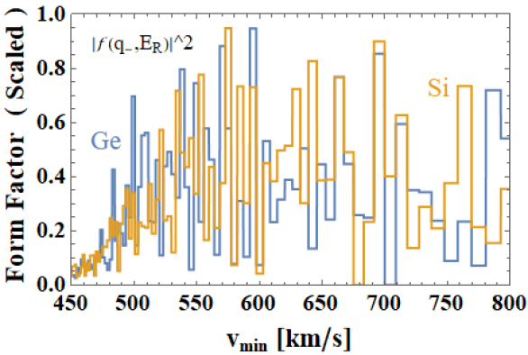
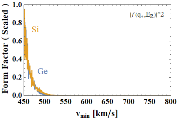
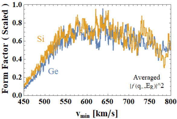
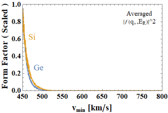
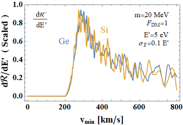
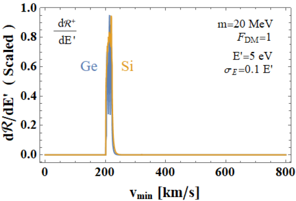
Figure 6: Comparison of Ge and Si electron form factors $|f_{\rm crys}(q_{\pm}(v_{\rm min},E_{\rm R}),E_{\rm R})|^{2}$ in Eq. (50) (two upper rows) for $E_{\rm R}=10$ eV (top row) and average form factor in the $E_{\rm R}$ range 9 eV to 11 eV (middle row), and Ge and Si response functions ${\text{d}\mathcal{R}^{\pm}_{\rm crys}(v_{\rm min},E^{\prime})}/{\text{d}E^{\prime}}$ in Eq. (50) for $m=$ 20 MeV, $E^{\prime}=$ 5 eV, $\sigma_{E}=0.5$ eV and $F_{\rm DM}=1$ (bottom row), as function of $v_{\rm min}$ for both the $q_{-}$ branch (left column) and the $q_{+}$ branch (right column).

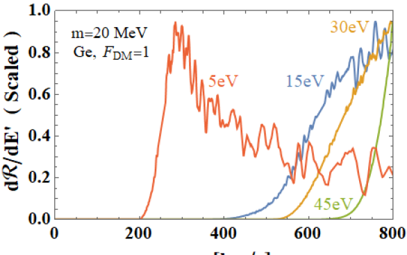
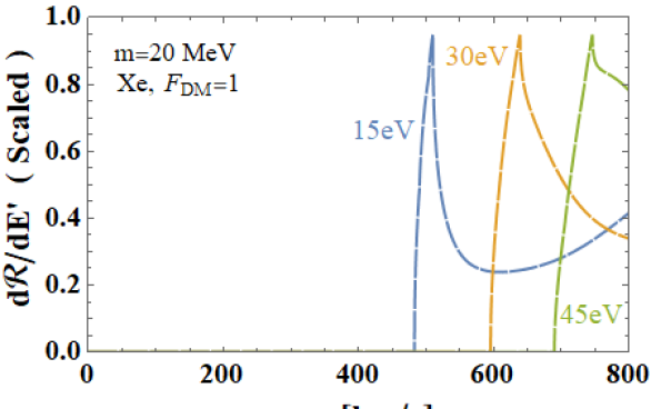
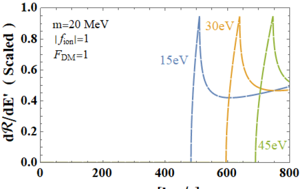
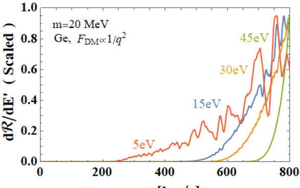
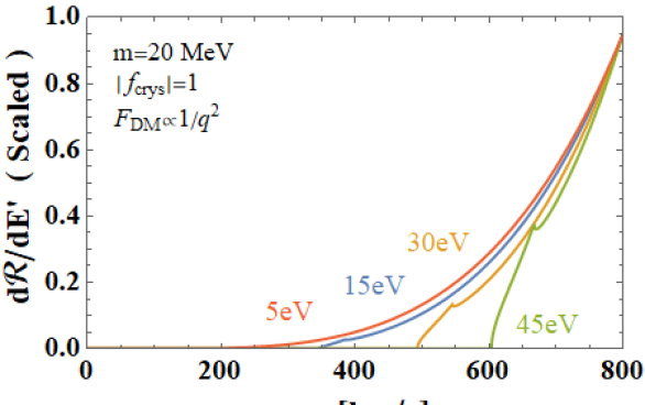
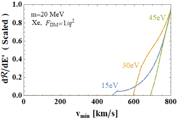
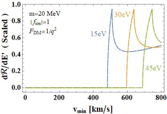
Figure 7: Response functions $d\mathcal{R}(v_{\rm min},E^{\prime})/dE^{\prime}$ for the time-average of $\tilde{\eta}(v_{\rm min},t)$ in Eq. (1) scaled by their maxima (so each ratio has a maximum $\simeq$ 1) for energies $E^{\prime}=$ 15, 30, and 45 eV and additionally $E^{\prime}=$5 eV for Ge (in Xe, the minimum detectable energy is 13.8 eV), for Ge (rows 1 and 3) and Xe detectors (rows 2 and 4), with actual electron form factors $|f^{i,f}|$ (left panels) and $|f^{i,f}|=1$ (right panels), $F_{\rm DM}=1$ (upper panels) and $\sim 1/q^{2}$ (lower panels), and $m=$20 MeV. Halo properties can be inferred from data only where $d\mathcal{R}/dE^{\prime}\neq 0$.

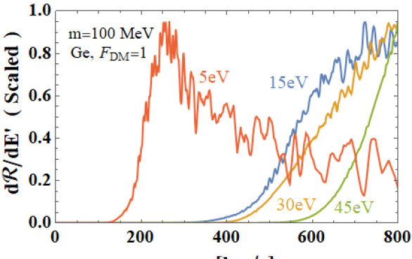
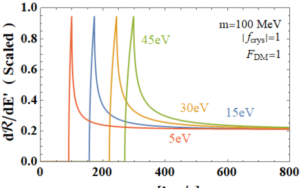
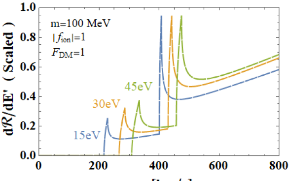
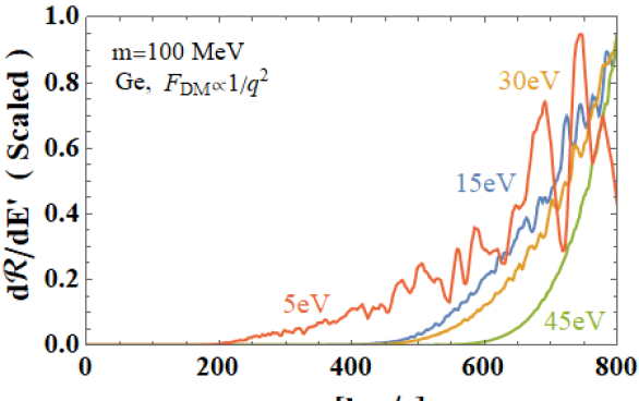
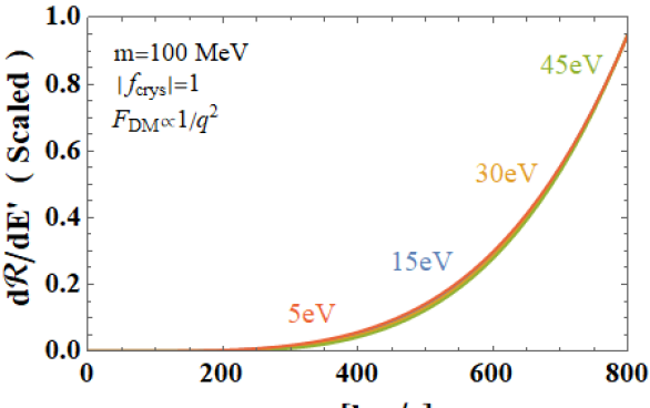
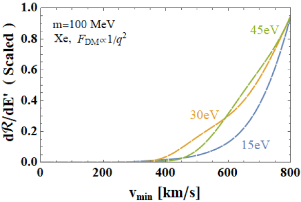
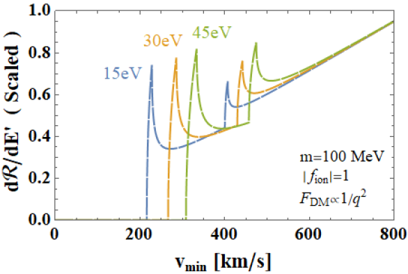
Figure 8: Same as Fig 7, but for a DM particle mass $m=$ 100 MeV.

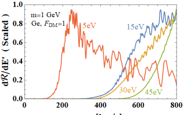
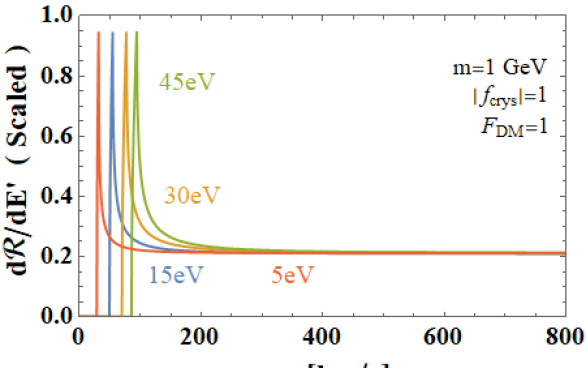
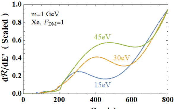
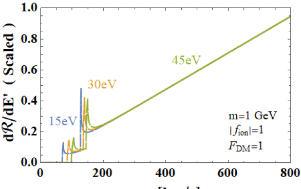
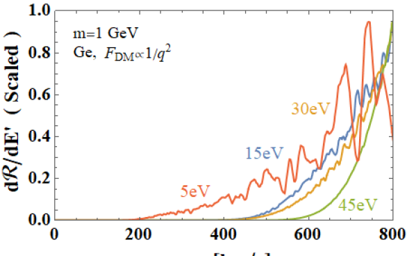
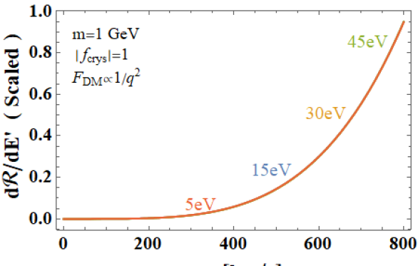
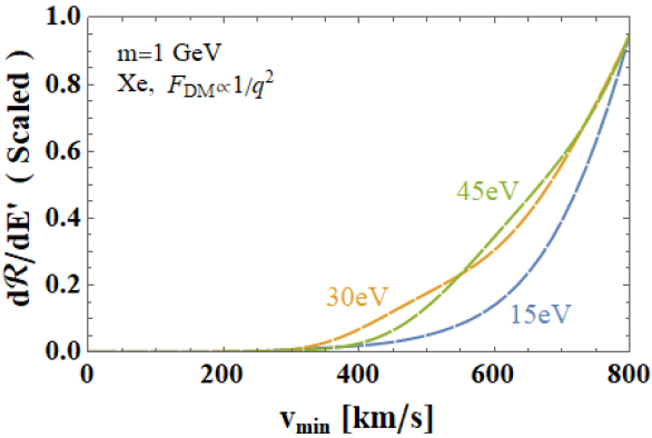
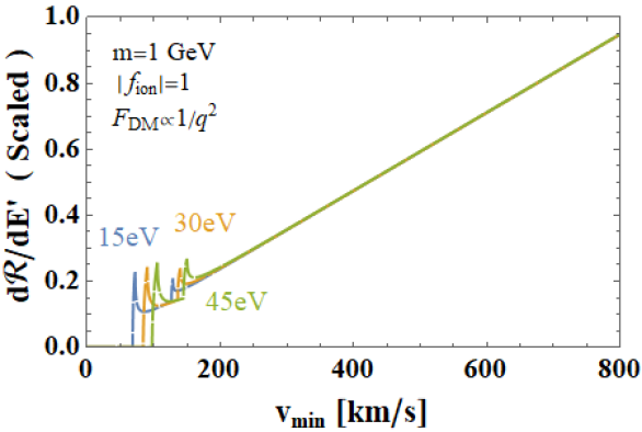
Figure 9: Same as Fig 7, but for a DM particle mass $m=$ 1 GeV.

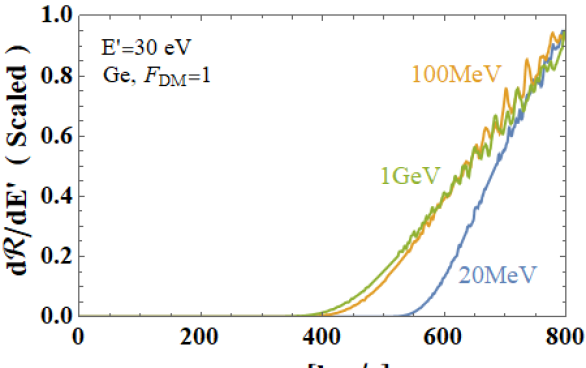
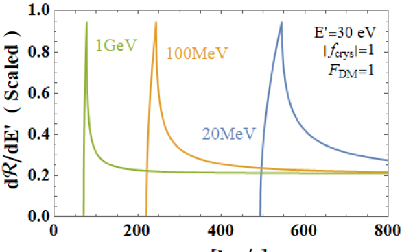
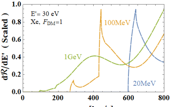
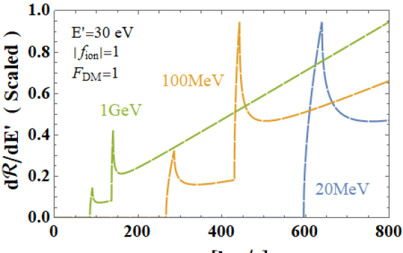
Figure 10: Response functions $d\mathcal{R}(v_{\rm min},E^{\prime})/dE^{\prime}$ for the time-average of $\tilde{\eta}(v_{\rm min},t)$ in Eq. (1) scaled by their maxima (so each ratio has a maximum $\simeq$ 1) for $F_{\rm DM}=1$ and energy $E^{\prime}=$ 30 eV, $\sigma_{E}=$ 3.0 eV and DM mass of 20 MeV, 100 MeV and 1 GeV, for Ge (row 1) and Xe detectors (rows 2), with the actual electron form factors $|f^{i,f}|$ in the left panels and $|f^{i,f}|=1$ in the right panels.

4 Results and Discussion

As we can see in Fig. 6, Si and Ge crystals have electron form factors $|f_{\rm crys}(q_{\pm},E_{\rm R})|^{2}$ in Eq. (50) (shown in the upper panels of Fig. 6) and response functions (shown in the bottom row) of similar shape. Thus, for our purpose it is sufficient to present results only for one of the two semiconductor materials, and we arbitrarily chose Ge.

Notice that in Fig. 6, as well as in the subsequent figures, Figs. 7 to 10, we are interested in showing the range of $v_{\rm min}$ where the response functions are different from zero, i.e. the range of $v_{\rm min}$ for which a particular experiment measuring events at a particular energy can give information about the DM halo local velocity distribution. Recall that the response function acts as a window function through which measured rates in direct detection experiments can provide information about the DM velocity (or speed) distribution. Since we are interested in the shape and not the magnitude of the functions, we show all of them divided by their maximum value, hence in our plots we show these dimensionless ratios with maximum value close to 1.

Figs. 7, 8 and  9 display the response functions $\text{d}\mathcal{R}/\text{d}E^{\prime}$ for the time-average of $\tilde{\eta}(v_{\rm min},t)$ in Eq. (1) as functions of $v_{\rm min}$, in Xe and Ge detectors, for DM particle masses of 20 MeV, 100 MeV and 1 GeV respectively and for two different DM form factors. We show these functions up to a maximum $v_{\rm min}$ value of $v_{\rm max}=$ 800 km/s, however our formalism can be trivially extended to larger $v_{\rm max}$ to account for a possible contribution of DM not bound to the Galaxy. These figures show the response functions for Ge (rows 1 and 3) and Xe detectors (rows 2 and 4) assuming realistic detected energy values $E^{\prime}=$15, 30 and 45 eV and additionally $E^{\prime}=$5 eV for Ge (in Xe, the minimum detectable energy is 13.8 eV). The four upper panels are for a DM form factor $F_{\rm DM}=1$, and the four lower panels assume $F_{\rm DM}\propto 1/q^{2}$. Eq. (55) and Eq. (57) show the effect of these different DM form factors in the $v_{\rm min}$ dependence of the response functions. The actual electron form factors $|f^{i,f}|$ are used in the left panels, but the electron form factors are set to 1, $|f^{i,f}|=1$, in the right columns. Thus the comparison of the left and right panels of every row allows to easily understand the impact the actual electron form factors have on the shape of the response functions. The electron form factors significantly affect the response functions shape, moving their maxima and thresholds to larger $v_{\rm min}$ values. In semiconductor crystals, they also introduce significant small scale variability in the function.

The double peaked structure of the Xe response functions seen in the right panels of Figs. 8 and  9 is due to the inclusion of only the 4d and 5p initial electron orbitals in our numerical evaluations. These are the two orbitals that contribute dominantly to the response functions (as shown in Fig. 4). The double peaked form in not present in Fig. 7 because for $m=20$ MeV only the 4d orbital contributes for $v_{\rm min}<800$ km/s.

In all our figures we chose to parameterize the experimental energy resolution as a box function of width $2\sigma_{\rm E}$ centered at the measured energy $E^{\prime}$. In Figs. 7 to 10 we chose $\sigma_{\rm E}=0.10E^{\prime}$. Similar results are obtained with other forms for this function, such as a Gaussian.

With our choice of energy resolution, the minimum $v_{\rm min}$ value for which the resolution function is non-zero in each case is $\tilde{v}=\sqrt{2(E^{\prime}-\sigma_{\rm E}+E_{\rm B})/m}$ (the function $\tilde{v}(E_{e})$ is defined in Eq. (26)), which decreases as $E^{\prime}$ decreases and as $m$ increases. Fig. 10 shows how the $v_{\rm min}$ threshold decreases with increasing DM particle mass, for a fixed $E^{\prime}=30$ eV in Ge and Xe. The kinematic effect of $E_{\rm B}\neq 0$ is clearly seen in the right panels of Fig. 10, where the electron form factors are taken to be 1. When the actual form factors are considered they affect considerably the $v_{\rm min}$ thresholds (the minimum value of $v_{\rm min}$ for which a response function is significantly different from zero). Only for DM masses close to 10 MeV (see our plots for $m=20$ MeV), due to the initial binding energy $E_{\rm B}$ in Xe, for the same DM particle model and $E^{\prime}$ the $v_{\rm min}$ threshold is lower in Ge and Si detectors than in Xe detectors. Instead, for larger masses (e.g. $m=100$ MeV and 1 GeV) the electron form factors make the $v_{\rm min}$ threshold lower in Xe than in Ge and Si for the same DM mass and $E^{\prime}$, although the effect is much less pronounced for $F_{\rm DM}\sim 1/q^{2}$ than for $F_{\rm DM}=1$. However, $E^{\prime}$ itself can be lower in semiconductor detectors, leading always to a smaller $v_{\rm min}$ threshold in Ge and Si than in Xe for the same particle model.

Thus, in general, Si and Ge detectors extend to lower $v_{\rm min}$ values, than Xe detectors. However, this advantage of semiconductor based detectors diminishes for larger DM mass values. As an example, see in the top panels of Fig. 9 that for $m=1$ GeV the $v_{\rm min}$ threshold for $E^{\prime}=5$ eV in Ge and that for $E^{\prime}>15$ eV in Xe are both about 100 km/s in the left panels.

The response functions act also as a weight, indicating the range of $v_{\rm min}$ from which potential DM signal mostly originates. The most likely speeds of the DM producing the observed rate are those for which the response function is larger. Conversely, therefore, the DM halo function is more precisely determined in the $v_{\rm min}$ regions where the response function is larger. The figures show that for $F_{\rm DM}\propto 1/q^{2}$ the response functions weigh more the high speed tail of the halo function. Although here we considered only elastic scattering off electrons our results can be easily transferred to the case of inelastic scattering, as explained in Sec. 3.4.

5 Conclusions

We have shown how to extend to DM scattering off electrons the halo-independent direct detection data analysis, so far developed for and only applied to DM scattering off nuclei.

A halo-independent analysis relies on the separation of the astrophysical parameters from the particle physics and detector dependent quantities. Namely, the method relies on expressing the predicted rate as a convolution of a function which depends only on the local DM distribution and density, and is thus common to all direct detection experiments, and a detector and DM particle model dependent kernel, which we call response function. The latter is non zero only for a limited range of DM particle speed (when considering just time-average rates and isotropic interactions, otherwise the response function depends on the DM velocity vector), which depends on the detected energy. Thus, the response function acts as a window through which direct detection data can give information on the local dark halo. Particular detectors can only provide information on the DM velocity distribution in a limited range of speeds depending on their characteristics. Thus complementarity of different experiments sensitive to partially overlapping velocity ranges would be needed to enable a more detailed inference of the DM distribution.

We showed here the general definitions of the response functions for DM scattering off electrons for time-averaged rates and discussed the differences and similarities with the case of scattering off nuclei. As illustrations of the procedure, using the electron form factors provided in Ref. Essig:2015cda , we computed numerically the response functions for ionization of xenon atoms and excitation of electrons in silicon and germanium crystals. We showed the range of DM speeds that experiments using these materials can be sensitive to, for different DM particle masses, and for realistic detected energies and experimental energy resolutions. In general, experiments using semiconductor targets can have smaller energy thresholds and thus reach smaller DM speeds, while xenon based experiments due to their larger exposure would allow for a more precise determination of the halo properties in the speed range where they are sensitive. Thus these two types of experiments are complementary.

The particular response functions we computed are those which correspond to the time-average of the halo function $\tilde{\eta}(v_{\rm min},t)$ (see Eq. (1)). However, in the halo-independent method any integral of the DM speed (or velocity, in more complicated situations) can be used to characterize the halo, taking into account that any likelihood used to fit a halo function to direct detection data can be maximized by a DM speed (or velocity) distribution written as a linear combination of delta functions, with a maximum number of terms given by the number of data points.

Appendix A Derivation of the general response function

The event rate of collisions in which an electron jumps from an initial state $i$ to a final state $f$ with energy difference $\Delta E_{i\rightarrow f}$ equal to the energy $E_{e}$ lost by the DM particle is

$$R_{i\rightarrow f}=\frac{\rho}{m}\int\text{d}^{3}v\,f_{\chi}(\vec{v})\langle\sigma v\rangle_{i\rightarrow f}~{},$$ (59)

where,

$$\langle\sigma v\rangle_{i\rightarrow f}=\frac{\overline{\sigma}_{e}}{4\pi\mu^{2}_{\chi e}}\int\text{d}^{3}q\,\delta(\Delta E_{i\rightarrow f}-\frac{q^{2}}{2m}+qv\cos\theta_{qv})|F_{\rm DM}(q)|^{2}|f_{i\rightarrow f}(\vec{q})|^{2}~{}.$$ (60)

Not all of the energy $E_{e}$ given to the electron in the collision is detectable. We call $E_{\rm R}$ the detectable energy, and

$$E_{\rm R}=\Delta E_{i\rightarrow f}-E_{{\rm B}i}~{}.$$ (61)

$E_{\rm R}$ is the electron recoil energy if electrons are free in the final state, e.g. electrons in an atom that is ionized, for which $E_{{\rm B}i}$ is the initial binding energy. Instead, neglecting very small energy losses, such as thermal dissipation via phonons, we take $E_{\rm R}=E_{e}$ for electrons scattering within a crystal. This condition can be written as a delta function

$$1=\int\text{d}E_{\rm R}\,\delta(E_{\rm R}-\Delta E_{i\rightarrow f}+E_{{\rm B}i})~{},$$ (62)

which is incorporated in the particular transition rate,

$$R_{i\rightarrow f} = \frac{\rho}{m}\frac{\overline{\sigma}_{e}}{4\pi\mu^{2}_{\chi e}}\int\text{d}^{3}v\,\text{d}^{3}q\,\text{d}E_{\rm R}\,\delta(E_{\rm R}+E_{{\rm B}i}-\frac{q^{2}}{2m}+qv\cos\theta_{qv})f_{\chi}(\vec{v})$$ (63)

$$\times\delta(E_{\rm R}-\Delta E_{i\rightarrow f}+E_{{\rm B}i})|F_{\rm DM}(q)|^{2}|f_{i\rightarrow f}(\vec{q})|^{2}~{}.$$

Then, summing over all possible occupied initial states and final states, the total rate is

$$R = \sum_{i,f}\frac{\rho}{m}\frac{\overline{\sigma}_{e}}{4\pi\mu^{2}_{\chi e}}\int\text{d}^{3}v\,\text{d}^{3}q\,\text{d}\ln E_{\rm R}\,\delta(E_{\rm R}+E_{{\rm B}i}-\frac{q^{2}}{2m}+qv\cos\theta_{qv})f_{\chi}(\vec{v})$$ (64)

$$\times E_{\rm R}\delta(E_{\rm R}-\Delta E_{i\rightarrow f}+E_{{\rm B}i})|F_{\rm DM}(q)|^{2}|f_{i\rightarrow f}(\vec{q})|^{2}~{}.$$

Here the summations represent integrations over continuous quantum numbers and actual summations over the discrete ones. The summation can be separated into sums over energy levels (indicated with a prime) and sums over all degenerate states,

$$\sum_{i}\sum_{f}=\sideset{}{{}^{\prime}}{\sum}_{i,f}\times\sum_{\begin{subarray}{c}\rm degen.\\ \rm states\end{subarray}}~{}.$$ (65)

The sum of the electron form factors $|f_{i\rightarrow f}(\vec{q})|^{2}$ over degenerate states which we call $|f^{i,f}|^{2}$, includes summing over all directions. Thus, there is no angular dependence left in $|f^{i,f}|^{2}$. Therefore, the sum can depend only on $q=|\vec{q}|$ (this is Eq. (33))

$$|f^{i,f}(q,E_{\rm R})|^{2}=\sum_{\begin{subarray}{c}\rm degen.\\ \rm states\end{subarray}}E_{\rm R}~{}\delta(E_{\rm R}-\Delta E_{i\rightarrow f}+E_{{\rm B}i})|f_{i\rightarrow f}(\vec{q})|^{2}~{}.$$ (66)

Using the following relation

$$\delta(E_{\rm R}+E_{{\rm B}i}-\frac{q^{2}}{2m}+qv\cos\theta_{qv})=\frac{1}{qv}\delta(\cos\theta_{qv}-\frac{v_{\rm min}}{v})~{},$$ (67)

we can perform the momentum integral over the solid angle $\Omega_{qv}$ in the rate to get

$$R = \sideset{}{{}^{\prime}}{\sum}_{i,f}\frac{1}{2\mu^{2}_{\chi e}}\int\text{d}\ln E_{\rm R}\int\text{d}q\,|F_{\rm DM}(q)|^{2}|f^{i,f}(q,E_{\rm R})|^{2}q$$ (68)

$$\times\left\{\frac{\rho\overline{\sigma}_{e}}{m}\int\text{d}^{3}v\,\frac{1}{v}\Theta(v-v_{\rm min}(q,E_{\rm R}+E_{{\rm B}i}))f_{\chi}(\vec{v})\right\}~{}.$$

The term inside the curly brackets in this equation is $\tilde{\eta}(v_{\rm min}(q,E_{\rm R}+E_{{\rm B}i}))$, the time-average of the function defined in Eq. (1) with the reference cross section $\sigma_{\rm ref}=\overline{\sigma}_{e}$. Thus, the general equation for the differential rate is

$$\frac{\text{d}R}{\text{d}E_{\rm R}}=\frac{1}{2\mu^{2}_{\chi e}}\frac{1}{E_{\rm R}}\sideset{}{{}^{\prime}}{\sum}_{i,f}\int\text{d}q\,\tilde{\eta}(v_{\rm min}(q,E_{\rm R}+E_{{\rm B}i}))|F_{\rm DM}(q)|^{2}|f^{i,f}(q,E_{\rm R})|^{2}q~{}.$$ (69)

Appendix B Electron form factor for DM scattering off electrons in an atom

In an atom target, the initial bound states are labeled by the principal quantum number $n$ and the angular momentum quantum number $l$, $|i\rangle=|nl\rangle$. If after the collision the atom is ionized, the final states are free spherical wave states labeled by $|f\rangle=|k^{\prime}l^{\prime}m^{\prime}\rangle$, where $k^{\prime}$ is the magnitude of the free electron momentum and $m^{\prime},l^{\prime}$ are spherical harmonic labels ($l^{\prime}$, $m^{\prime}$ labeled states are degenerate for the same $k^{\prime}$). Thus, the form factor $|f_{i\to f}(\vec{q})|$ in Eq. (64) is now

$$|f_{i\rightarrow f}(\vec{q})|^{2}=|f_{nl\rightarrow k^{\prime}l^{\prime}m^{\prime}}(\vec{q})|^{2}=\left|\int\text{d}^{3}x\,\psi_{k^{\prime}l^{\prime}m^{\prime}}^{*}(\vec{x})\psi_{nl}(\vec{x})e^{i\vec{q}\cdot\vec{x}}\right|^{2}~{},$$ (70)

and the summation over states given in Eq. (65) becomes

$$\sum_{i,f}=\sum_{nl}\sum_{\begin{subarray}{c}\rm degen.\\ \rm states\end{subarray}}\int\frac{k^{\prime 2}\text{d}k^{\prime}}{(2\pi)^{3}}~{}.$$ (71)

Summed over all final states, the form factor given in Eq. (66) becomes

$$\int\frac{k^{\prime 2}\text{d}k^{\prime}}{(2\pi)^{3}}\,|f^{nl,k^{\prime}}_{\rm ion}(q,E_{\rm R})|^{2} = \sum_{\begin{subarray}{c}\rm degen.\\ \rm states\end{subarray}}\int\frac{k^{\prime 2}\text{d}k^{\prime}}{(2\pi)^{3}}\,E_{\rm R}\delta(E_{\rm R}-\Delta E_{nl\rightarrow k^{\prime}l^{\prime}m^{\prime}}+E_{{\rm B}nl})$$

$$\times\left|\int\text{d}^{3}x\,\psi_{k^{\prime}l^{\prime}m^{\prime}}^{*}(\vec{x})\psi_{nl}(\vec{x})e^{i\vec{q}\cdot\vec{x}}\right|^{2}$$

Since the recoil energy is

$$E_{\rm R}^{\prime}=\frac{k^{\prime 2}}{2m_{e}}=\Delta E_{nl\rightarrow k^{\prime}l^{\prime}m^{\prime}}-E_{{\rm B}nl}~{},$$ (73)

we have

$$\int\frac{k^{\prime 2}\text{d}k^{\prime}}{(2\pi)^{3}} |f^{nl,k^{\prime}}_{\rm ion}(q,E_{\rm R})|^{2}=\sum_{\begin{subarray}{c}\rm degen.\\ \rm states\end{subarray}}\int\frac{k^{\prime 3}\text{d}\ln E_{\rm R}^{\prime}}{2(2\pi)^{3}}\,E_{\rm R}\delta(E_{\rm R}-E_{\rm R}^{\prime})\left|\int\text{d}^{3}x\,\psi_{k^{\prime}l^{\prime}m^{\prime}}^{*}(\vec{x})\psi_{nl}(\vec{x})e^{i\vec{q}\cdot\vec{x}}\right|^{2}$$ (74)

$$= \sum_{\begin{subarray}{c}\rm degen.\\ \rm states\end{subarray}}\,\frac{k^{\prime 3}}{2(2\pi)^{3}}\left|\int\text{d}^{3}x\,\psi_{k^{\prime}l^{\prime}m^{\prime}}^{*}(\vec{x})\psi_{nl}(\vec{x})e^{i\vec{q}\cdot\vec{x}}\right|^{2}=\dfrac{1}{4}|f_{\rm ion}^{nl}(q,E_{\rm R})|^{2}~{}.$$

Where we have used the definition of the form factor given in Eq.(6) of Ref. Essig:2011nj ,

$$|f_{\rm ion}^{nl}(q,E_{\rm R})|^{2}=\sum_{\begin{subarray}{c}\rm degen.\\ \rm states\end{subarray}}\,\frac{2k^{\prime 3}}{(2\pi)^{3}}\left|\int\text{d}^{3}x\,\psi_{k^{\prime}l^{\prime}m^{\prime}}^{*}(\vec{x})\psi_{nl}(\vec{x})e^{i\vec{q}\cdot\vec{x}}\right|^{2}.$$ (75)

Appendix C Electron form factor for DM scattering off electrons in a crystals

In crystals, a DM particle excites an electron from a Bloch state $|{n\vec{k}}\rangle$ to another Bloch state $|{n^{\prime}\vec{k}^{\prime}}\rangle$, where $n$ and $n^{\prime}$ are the band index labels in the first Brillouin Zone (BZ). Thus, the form factor $|f_{i\to f}(\vec{q})|$ in Eq. (64) is

$$|f_{i\rightarrow f}(\vec{q})|^{2}=|f_{n\vec{k}\rightarrow n^{\prime}\vec{k}^{\prime}}(\vec{q})|^{2}=\left|\int\text{d}^{3}x\,\psi_{n^{\prime}\vec{k}^{\prime}}^{*}(\vec{x})\psi_{n\vec{k}}(\vec{x})e^{i\vec{q}\cdot\vec{x}}\right|^{2}~{}.$$ (76)

The Bloch state wavefunctions $\psi_{n\vec{k}}$ are

$$\psi_{n\vec{k}}(\vec{x})=\dfrac{1}{\sqrt{V}}\sum_{\vec{G}}u_{n}(\vec{k}+\vec{G})e^{i(\vec{k}+\vec{G})\cdot\vec{x}}~{},$$ (77)

where the summation is over all reciprocal lattice vectors $\vec{G}$, $V$ is the volume of the crystal, and $u_{n}$ are normalized wavefunctions satisfying

$$\sum_{\vec{G}}|u_{n}(\vec{k}+\vec{G})|^{2}=1~{}.$$ (78)

Thus,

$$|f_{n\vec{k}\rightarrow n^{\prime}\vec{k}^{\prime}}(\vec{q})|^{2}=\left|\int\text{d}^{3}x\,\frac{1}{V}\sum_{\vec{G}^{\prime}}u^{*}_{n^{\prime}}(\vec{k}^{\prime}+\vec{G}^{\prime})e^{i(\vec{k}^{\prime}+\vec{G}^{\prime})\cdot\vec{x}}\sum_{\vec{G}}u_{n}(\vec{k}+\vec{G})e^{i(\vec{k}+\vec{G})\cdot\vec{x}}e^{i\vec{q}\cdot\vec{x}}~{}\right|^{2}~{}.$$ (79)

For crystal dimensions much larger than the atomic separation (we consider only large detectors where the interactions happen in the volume and surface effects are negligible) the discrete crystal momentum $\vec{k}$ can be approximated by a continuous variable, thus

$$\int\text{d}^{3}x~{}e^{i\vec{k}\cdot\vec{x}}=(2\pi)^{3}\delta^{3}(\vec{k})~{},$$ (80)

and the summation over states in Eq. (65) becomes

$$\sum_{i,f}=2\sum_{nn^{\prime}}\int_{\rm BZ}\frac{V\text{d}^{3}k}{(2\pi)^{3}}\frac{V\text{d}^{3}k^{\prime}}{(2\pi)^{3}}~{}.$$ (81)

Here, the extra factor of 2 comes from summing over degenerate spin states. Since the summation in Eq. (77) is over all reciprocal vectors,

$$\frac{1}{\sqrt{V}}\sum_{\vec{G}^{\prime}}u_{n}(\vec{k}^{\prime}+\vec{G}^{\prime})e^{i(\vec{k}^{\prime}+\vec{G}^{\prime})\cdot\vec{x}}=\frac{1}{\sqrt{V}}\sum_{\vec{G}^{\prime}}u_{n}(\vec{k}^{\prime}+\vec{G}^{\prime}+\vec{G})e^{i(\vec{k}^{\prime}+\vec{G}^{\prime}+\vec{G})\cdot\vec{x}}~{},$$ (82)

using Eq. (80), one can write the form factor in Eq. (79) as

$$|f_{n\vec{k}\rightarrow n^{\prime}\vec{k}^{\prime}}(\vec{q})|^{2}=\left|\sum_{\vec{G}}\sum_{\vec{G}^{\prime}}\frac{(2\pi)^{3}}{V}\delta^{3}(\vec{k}+\vec{q}-\vec{k}^{\prime}-\vec{G}^{\prime})u^{*}_{n^{\prime}}(\vec{k}^{\prime}+\vec{G}^{\prime}+\vec{G})u_{n}(\vec{k}+\vec{G})\right|^{2}~{}.$$ (83)

Since all other terms in Eq. (69) besides the electron form factors are independent of the choice of $i$ and $f$ states, as a result of taking $E_{{\rm B}i}=0$, the summation over initial and final states with different energy only affects the electron form factors, and this sum is

$$\sideset{}{{}^{\prime}}{\sum}_{i,f}|f^{i,f}(q,E_{\rm R})|^{2}=2\sum_{nn^{\prime}}\int_{\rm BZ}\frac{V\text{d}^{3}k}{(2\pi)^{3}}\frac{V\text{d}^{3}k^{\prime}}{(2\pi)^{3}}\,E_{\rm R}\delta(E_{\rm R}-\Delta E_{n\vec{k}\rightarrow n^{\prime}\vec{k}^{\prime}})|f_{n\vec{k}\rightarrow n^{\prime}\vec{k}^{\prime}}(\vec{q})|^{2}~{}.$$ (84)

The summation in Eq. (84) includes a summation over directions, thus the result is independent of the direction of $\vec{q}$, a result which can be incorporated into Eq. (84) by replacing in it $|f_{n\vec{k}\rightarrow n^{\prime}\vec{k}^{\prime}}(\vec{q})|^{2}$ by

$$\int\text{d}^{3}p\,\delta^{3}(\vec{p}-\vec{q})|f_{n\vec{k}\rightarrow n^{\prime}\vec{k}^{\prime}}(\vec{p})|^{2}=\int\dfrac{\text{d}^{3}p}{4\pi p^{2}}\delta(p-q)|f_{n\vec{k}\rightarrow n^{\prime}\vec{k}^{\prime}}(p)|^{2}~{}.$$ (85)

Eq. (84) becomes

$$\sideset{}{{}^{\prime}}{\sum}_{i,f}|f^{i,f}(q,E_{\rm R})|^{2} = \int\dfrac{\text{d}^{3}p}{2\pi p^{2}}\,\delta(p-q)\sum_{nn^{\prime}}\int_{\rm BZ}\frac{V^{2}\text{d}^{3}k\,\text{d}^{3}k^{\prime}}{(2\pi)^{6}}\,E_{\rm R}\delta(E_{\rm R}-\Delta E_{n\vec{k}\rightarrow n^{\prime}\vec{k}^{\prime}})|f_{n\vec{k}\rightarrow n^{\prime}\vec{k}^{\prime}}(p)|^{2}$$ (86)

$$= \frac{4\pi^{2}}{q^{3}V}\sum_{nn^{\prime}}\int_{\rm BZ}\frac{V\text{d}^{3}k}{(2\pi)^{3}}\frac{V\text{d}^{3}k^{\prime}}{(2\pi)^{3}}\,E_{\rm R}\delta(E_{\rm R}-\Delta E_{n\vec{k}\rightarrow n^{\prime}\vec{k}^{\prime}})$$

$$\times\sum_{\vec{G}^{\prime}}\,q\delta(q-|\vec{k}^{\prime}+\vec{G}^{\prime}-\vec{k}|)\left|\sum_{\vec{G}}u^{*}_{n^{\prime}}(\vec{k}^{\prime}+\vec{G}^{\prime}+\vec{G})u_{n}(\vec{k}+\vec{G})\right|^{2}.$$

Expressing the total volume in terms of the volume $V_{\rm cell}$ of one cell, $V=N_{\rm cell}V_{\rm cell}$,

$$\sideset{}{{}^{\prime}}{\sum}_{i,f}|f^{i,f}(q,E_{\rm R})|^{2} = \frac{4\pi^{2}N_{\rm cell}}{q^{3}V_{\rm cell}}\sum_{nn^{\prime}}\int_{\rm BZ}\frac{V_{\rm cell}\,\text{d}^{3}k}{(2\pi)^{3}}\frac{V_{\rm cell}\,\text{d}^{3}k^{\prime}}{(2\pi)^{3}}\,E_{\rm R}\delta(E_{\rm R}-\Delta E_{n\vec{k}\rightarrow n^{\prime}\vec{k}^{\prime}})$$ (87)

$$\times\sum_{\vec{G}^{\prime}}\,q\delta(q-|\vec{k}^{\prime}+\vec{G}^{\prime}-\vec{k}|)\left|\sum_{\vec{G}}u^{*}_{n^{\prime}}(\vec{k}^{\prime}+\vec{G}^{\prime}+\vec{G})u_{n}(\vec{k}+\vec{G})\right|^{2}$$

$$= \frac{2N_{\rm cell}E_{\rm R}}{q^{3}}(\alpha m_{e}^{2})|f_{\rm crys}(q,E_{\rm R})|^{2}~{},$$

where

$$|f_{\rm crys}(q,E_{\rm R})|^{2} = \frac{2\pi^{2}}{\alpha m_{e}^{2}}\frac{1}{V_{\rm cell}E_{\rm R}}\sum_{nn^{\prime}}\int_{\rm BZ}\frac{V_{\rm cell}\,\text{d}^{3}k}{(2\pi)^{3}}\,\frac{V_{\rm cell}\,\text{d}^{3}k^{\prime}}{(2\pi)^{3}}\,E_{\rm R}\delta(E_{\rm R}-\Delta E_{n\vec{k}\rightarrow n^{\prime}\vec{k}^{\prime}})$$ (88)

$$\times\sum_{\vec{G}^{\prime}}q\delta(q-|\vec{k}^{\prime}+\vec{G}^{\prime}-\vec{k}|)\left|\sum_{\vec{G}}u^{*}_{n^{\prime}}(\vec{k}^{\prime}+\vec{G}^{\prime}+\vec{G})u_{n}(\vec{k}+\vec{G})\right|^{2}~{}.$$

is the crystal form factor defined in Eq. (A.33) of Ref. Essig:2015cda .

Appendix D Expression for numerical calculations of the response function for general a, b and c constants

We use the computed electron form factors of Ref. Essig:2015cda for Xe, Ge and Si target, but our analysis is general and our treatment is readily applicable to any given electron form factors that can be described by binned data with a power law dependency of $q^{a}$ and $E_{\rm R}^{b}$, where $a,b$ are integers, so that

$$|f^{i,f}(q_{\pm},E_{\rm R})|^{2}=q_{\pm}^{a}E_{\rm R}^{b}|f^{i,f}_{\rm dat}(E_{\rm R},q_{\pm})|^{2}~{}.$$ (89)

In the particular cases we consider in this paper, $a=-3$ and $b=1$ for crystals (see Eq. (56)) and $a=b=0$ for an atom (see Eq. (53)). Writing additionally $|F_{\rm DM}(q)|^{2}=(\alpha m_{e})^{2c}q^{-2c}$, where either $c=0$ or $c=2$ are our two choices, the response function integral to be evaluated in Eq. (39) takes the functional form

$$\frac{d\mathcal{R}_{\pm}}{dE^{\prime}}(v_{\rm min},E^{\prime}) = \frac{\epsilon(E^{\prime})}{4\mu_{\chi e}^{2}\sigma_{\rm E}}(\alpha m_{e})^{2c}\sideset{}{{}^{\prime}}{\sum}_{i,f}\int_{E^{\prime}-\sigma_{\rm E}}^{E_{\rm max}}\text{d}E_{\rm R}\,E_{\rm R}^{b-1}~{}q^{a+1-2c}_{\pm}(v_{\rm min},E_{\rm R}+E_{{\rm B}i})~{}$$ (90)

$$\times J_{\pm}(v_{\rm min},E_{\rm R}+E_{{\rm B}i})|f^{i,f}_{\rm dat}(E_{\rm R},q_{\pm}(v_{\rm min},E_{\rm R}+E_{{\rm B}i}))|^{2}~{}.$$

Extracting the constant data value for the electron form factor in each bin and performing the remaining integral analytically, the expression we compute numerically is

$$\frac{d\mathcal{R_{\pm}}}{dE^{\prime}}=\frac{\epsilon(E^{\prime})}{4\mu_{\chi e}^{2}\sigma_{\rm E}}(\alpha m_{e})^{2c}\sideset{}{{}^{\prime}}{\sum}_{i,f}\sum_{{\rm Path}(r,s)}I^{\pm,i}_{abc}(v_{\rm min},E_{1}^{(rs)},E_{2}^{(rs)})~{}|f^{i,f}_{\rm dat}|^{2}_{rs}~{},$$ (91)

where the summation is over all the $(r,s)$ partitions through which the path described by the function $q(v_{\rm min},E_{\rm R})$ passes, as indicated in Fig. 5. The analytically computed $I^{\pm,i}_{abc}(E_{1}^{(rs)},E_{2}^{(rs)})$ integrals are

$$I^{\pm,i}_{abc}(v_{\rm min},E_{1}^{(rs)},E_{2}^{(rs)})=\int_{E_{1}^{(rs)}}^{E_{2}^{(rs)}}\dfrac{\text{d}E_{\rm R}}{E_{\rm R}^{1-b}}\,q^{a+1-2c}_{\pm}(v_{\rm min},E_{\rm R}+E_{{\rm B}i})J_{\pm}(v_{\rm min},E_{\rm R}+E_{{\rm B}i})~{}.$$ (92)

Here, $E_{1}^{(rs)}$ and $E_{2}^{(rs)}$ are the boundaries of the shaded area in the partition $(rs)$ shown in Fig. 5. Since the partitions are small, we use the approximation $E_{\rm R}\approx(E_{1}^{(rs)}+E_{2}^{(rs)})/2$ and take $E_{\rm R}^{b-1}$ outside the integral, so Eq. (92) becomes

$$I^{\pm,i}_{abc}(v_{\rm min},E_{1}^{(rs)},E_{2}^{(rs)})\simeq 2\int_{E_{1}^{(rs)}}^{E_{2}^{(rs)}}\text{d}E_{\rm R}\,\frac{q^{a+1-2c}_{\pm}(v_{\rm min},E_{\rm R}+E_{{\rm B}i})\,J_{\pm}(v_{\rm min},E_{\rm R}+E_{{\rm B}i})}{\left(E_{1}^{(rs)}+E_{2}^{(rs)}\right)^{1-b}}~{}.$$ (93)

Performing this integral we find: for $a-2c=-3$,

$$I^{\pm,i}_{abc}(v_{\rm min},E_{1}^{(rs)},E_{2}^{(rs)})\simeq\mp\left(\frac{E_{1}^{(rs)}+E_{2}^{(rs)}}{2}\right)^{b-1}\left.\left[\ln\left|1\pm\sqrt{1-\dfrac{2(E_{\rm R}+E_{{\rm B}i})}{mv_{\rm min}^{2}}}\right|\right]\right|_{E_{1}^{(rs)}}^{E_{2}^{(rs)}}~{};$$ (94)

for $a-2c\neq-3$,

$$I^{\pm,i}_{abc}(v_{\rm min},E_{1}^{(rs)},E_{2}^{(rs)}) \simeq \mp\left(\frac{E_{1}^{(rs)}+E_{2}^{(rs)}}{2}\right)^{b-1}\dfrac{(mv_{\rm min})^{a-2c+3}}{a-2c+3}$$

$$\times\left.\left[\left(1\pm\sqrt{1-\dfrac{2(E_{\rm R}+E_{{\rm B}i})}{mv_{\rm min}^{2}}}\right)^{a-2c+3}\right]\right|_{E_{1}^{(rs)}}^{E_{2}^{(rs)}}~{}.$$

Both of them are always positive.

Appendix E Alternative derivation of the response function for DM scattering off electrons

The response function $\text{d}\mathcal{R}/\text{d}E^{\prime}$ can be derived using the relation in Eq. (12)

$$\frac{\text{d}\mathcal{R}}{\text{d}E^{\prime}}(v_{\rm min},E^{\prime})\equiv\frac{\partial}{\partial v_{\rm min}}\left[\frac{\text{d}\mathcal{H}}{\text{d}E^{\prime}}(v_{\rm min},E^{\prime})\right]\,,$$ (96)

from the response function ${\text{d}\mathcal{H}}(v_{\rm min},E^{\prime})/{\text{d}E^{\prime}}$ to the speed distribution, when we write the rate as in Eq. (9), namely

$$\frac{\text{d}R}{\text{d}E^{\prime}}=\frac{\overline{\sigma}_{e}\rho}{m}\int_{0}^{\infty}{\rm d}v~{}\frac{F(v,t)}{v}\frac{{\rm d}\mathcal{H}}{{\rm d}E^{\prime}}(v,E^{\prime})\,.$$ (97)

This procedure allows us to make contact with the formulation used for DM scattering off nuclei, in particular for inelastic scattering, as explained in App F.

Starting from Eq. (64) and using Eq. (66) and Eq. (67) we get

$$\dfrac{\text{d}R}{\text{d}E_{\rm R}}=\sideset{}{{}^{\prime}}{\sum}_{i,f}\frac{\rho~{}\overline{\sigma}_{e}}{4\pi\mu^{2}_{\chi e}mE_{\rm R}}\int\text{d}^{3}vf_{\chi}(\vec{v})\int\frac{\text{d}^{3}q}{qv}\delta(\cos\theta_{qv}-\frac{v_{\rm min}}{v})|F_{\rm DM}(q)|^{2}|f^{i,f}(q,E_{\rm R})|^{2},$$ (98)

or after further simplification

$$\dfrac{\text{d}R}{\text{d}E_{\rm R}}=\sideset{}{{}^{\prime}}{\sum}_{i,f}\frac{\rho}{m}\frac{\overline{\sigma}_{e}}{2\mu^{2}_{\chi e}E_{\rm R}}\int_{\tilde{v}}\text{d}v\,\frac{F(v)}{v}\int_{q_{-}(v,E_{e})}^{q_{+}(v,E_{e})}\text{d}q\,q~{}|F_{\rm DM}(q)|^{2}~{}|f^{i,f}(q,E_{\rm R})|^{2}~{},$$ (99)

where $\tilde{v}=\sqrt{2E_{e}/m}$ and the functions $q_{\pm}(v,E_{e})$ are given in Eq. (25). Integrating now on $E_{\rm R}$ to obtain the observable differential rate ${\text{d}R}/{\text{d}E^{\prime}}$ we identify ${\text{d}\mathcal{H}}(E^{\prime},v)/{\text{d}E^{\prime}}$ as

$$\dfrac{\text{d}\mathcal{H}}{\text{d}E^{\prime}}(v,E^{\prime})\equiv\begin{dcases}\hfill\frac{\epsilon(E^{\prime})}{2\mu^{2}_{\chi e}}\int\frac{\text{d}E_{\rm R}}{E_{\rm R}}G(E^{\prime},E_{\rm R})\sideset{}{{}^{\prime}}{\sum}_{i,f}\int_{q_{-}(v,E_{e})}^{q_{+}(v,E_{e})}\text{d}q\,q|F_{\rm DM}(q)|^{2}|f^{i,f}(q,E_{\rm R})|^{2}\hfill&\text{ if $v\geqslant\tilde{v}$,}\\ &\\ \hfill 0\hfill&\text{ if $v<\tilde{v}$.}\\ \end{dcases}$$ (100)

Notice that this expression depends on the speed $v$ only though the limits of the integration in $q$. Taking the partial derivative of this expression with respect to $v$, and recalling we defined in Eq. (34) ${\partial q_{\pm}(v,E_{e})}/{\partial v}=J_{\pm}(v,E_{e})$, we recover Eqs. (38) and (39).

Appendix F Comparison with the formalism for DM scattering off nuclei

In DM-electron scattering, with kinematics described by Eq. (23), two of the three variables - momentum transfer $q$, detectable energy $E_{\rm R}$, and $v_{\rm min}$ - are independent. In the halo-dependent usual formalism, $v_{\rm min}$ is taken to be a function of the other two. In the halo-independent formalism, we choose instead $E_{\rm R}$ and $v_{\rm min}$ as independent variables, and thus we change an integration in $q$ to obtain the rate into an integration in $v_{\rm min}$.

In the DM scattering off nuclei (of mass $m_{N}$) the kinematics sets $E_{\rm R}=q^{2}/2m_{N}$, and only one of the two variables $E_{\rm R}$ and $v_{\rm min}$ is independent. In the halo-independent method we chose $v_{\rm min}$ to be the independent variable and thus change an integration in $E_{\rm R}$ to get the predicted event rate into an integration in $v_{\rm min}$.

In spite of these differences in the kinematics of DM-electron scattering and DM-nucleus scattering, we can identify a similarity in the equations we get in $q$ in DM scattering off electrons and in $E_{\rm R}$ in the inelastic endothermic DM scattering off nuclei. In this latter case, the DM particles scatter to a new state of mass $m^{\prime}=m+\delta$, where $|\delta|\ll m$, and $\delta>0$ ($<0$) describes endothermic (exothermic) scattering. In this case (see e.g. Refs. DelNobile:2013cva ; Gelmini:2015voa ; Gelmini:2016pei ), in the limit $\mu_{\chi N}|\delta|/m^{2}\ll 1$, $v_{\rm min}(E_{\rm R})$ is

$$v_{\rm min}(E_{\rm R})=\frac{1}{\sqrt{2m_{N}E_{\rm R}}}\left|\frac{m_{N}E_{\rm R}}{\mu_{\chi N}}+\delta\right|\,,$$ (101)

which reduces to the typical equation for elastic scattering when $\delta=0$. Thus, the range of possible recoil energies that can be imparted to a target nucleus by a DM particle traveling at speed $v$ in Earth’s frame is $[E_{\rm R}^{-}(v),E_{\rm R}^{+}(v)]$, where

$$E_{\rm R}^{\pm}(v)=\frac{\mu_{\chi N}^{2}v^{2}}{2m_{N}}\left(1\pm\sqrt{1-\frac{2\delta}{\mu_{\chi N}~{}v^{2}}}\right)^{2}\,.$$ (102)

For endothermic scattering the minimum possible value of $v$ is $v_{\delta}^{N}=\sqrt{2\delta/\mu_{\chi N}}>0$, which depends on the nuclide type through the reduced mass $\mu_{\chi N}$ (for exothermic and elastic scattering the minimum is instead $v_{\delta}=0$). Notice the similarity of the definition of $E_{\rm R}^{\pm}(v)$ in Eq. (102) with the definition of $q_{\pm}(v,E_{e})$ in Eq. (25). In Eq. (99), for a fixed speed $v$ the integration in $q$ is between $q_{-}$ and $q_{+}$, and similarly here the integration for fixed speed is between $E_{\rm R}^{-}$ and $E_{\rm R}^{+}$. The differential rate as a function of the detected energy $E^{\prime}$ for DM scattering off a nuclide $N$ is (see Eq. (4), Eq. (5), Eq. (8) and Eq. (9))

$$\frac{\text{d}R_{N}}{\text{d}E^{\prime}}=\epsilon(E^{\prime})\int_{0}^{\infty}\text{d}E_{\rm R}\,G_{N}(E^{\prime},E_{\rm R})\,\frac{\text{d}R_{N}}{\text{d}E_{\rm R}}~{}.$$ (103)

Thus, summing over all nuclides in the target the total rate can be written in the form

$$\frac{\text{d}R}{\text{d}E^{\prime}}=\frac{\sigma_{\text{ref}}\rho}{m}\int_{v\geqslant v_{\delta}}\text{d}^{3}v\,\frac{f_{\chi}(\vec{v},t)}{v}\,\frac{\text{d}\mathcal{H}}{\text{d}E^{\prime}}(\vec{v},E^{\prime})\,,$$ (104)

where the response function $\text{d}\mathcal{H}/{\text{d}E^{\prime}}=\sum_{N}\text{d}\mathcal{H}_{N}/{\text{d}E^{\prime}}$ (Eq. (10)) is DelNobile:2013cva ; Gelmini:2015voa ; Gelmini:2016pei

$$\frac{\text{d}\mathcal{H}}{\text{d}E^{\prime}}(\vec{v},E^{\prime})\equiv\begin{dcases}\hfill\sum_{N}N_{N}\int_{E_{\rm R}^{-}}^{E_{\rm R}^{+}}\,\text{d}E_{\rm R}\,\epsilon(E^{\prime},E_{\rm R})\,G_{N}(E_{\rm R},E^{\prime})\,\frac{v^{2}}{\sigma_{\text{ref}}}\,\frac{\text{d}\sigma_{N}}{\text{d}E_{\rm R}}(E_{\rm R},\vec{v})\hfill&\text{ if $v\geqslant v_{\delta}$,}\\ \hfill 0\hfill&\text{ if $v<v_{\delta}$.}\end{dcases}$$ (105)

Here, $N_{N}$ is the number of nuclei per unit mass of the detector, $\sigma_{N}$ is the DM-nucleus scattering cross section and $v_{\delta}$ is the smallest of the speed threshold values $v_{\delta}^{N}$ for all nuclides in the target. Notice the formal similarity between Eq. (105) and Eq. (100). Similarly to the response function in Eq. (100), the response function for nuclear scattering in Eq. (105) depends only on the speed $v$, instead of the velocity vector $\vec{v}$ if the scattering does not depend on the direction of the incoming DM particle.

As for DM scattering off electrons, also for inelastic endothermic scattering off nuclei for which $v_{\delta}\not=0$ (these are Eq. (11) to Eq. (15) applied to this type of DM)

$$\frac{\text{d}R}{\text{d}E^{\prime}}=-\int_{v_{\delta}}^{\infty}\text{d}v\,\frac{\partial\tilde{\eta}(v,t)}{\partial v}\,\frac{\text{d}\mathcal{H}}{\text{d}E^{\prime}}(v,E^{\prime})\,,$$ (106)

and, using that $\tilde{\eta}(\infty,t)=0$ and $\text{d}\mathcal{H}/\text{d}E^{\prime}(E^{\prime},v_{\delta})=0$, integrating Eq. (106) by parts results in

$$\frac{\text{d}R}{\text{d}E^{\prime}}=\int_{v_{\delta}}^{\infty}\text{d}v_{\rm min}\tilde{\eta}(v_{\rm min},t)\,\frac{\text{d}\mathcal{R}}{\text{d}E^{\prime}}(v_{\rm min},E^{\prime})\,,$$ (107)

where the differential response function $\text{d}\mathcal{R}/\text{d}E^{\prime}$ is

$$\frac{\text{d}\mathcal{R}}{\text{d}E^{\prime}}(v_{\rm min},E^{\prime})\equiv\frac{\partial}{\partial v_{\rm min}}\left[\frac{\text{d}\mathcal{H}}{\text{d}E^{\prime}}(v_{\rm min},E^{\prime})\right]\,.$$ (108)

As for DM scattering off electrons, here if $v_{\delta}$ is in the observable range of an experiment, the response function ${\text{d}\mathcal{R}}{\text{d}E^{\prime}}$ depends on a Jacobian factor $\partial{E_{\rm R}}^{\pm}/\partial E_{\rm R}$ which is singular at $v=v_{\delta}$.

References

- (1) G. Bertone, D. Hooper and J. Silk, Particle dark matter: Evidence, candidates and constraints, Phys. Rept. 405 (2005) 279 [hep-ph/0404175].
- (2) J. L. Feng and J. Kumar, The WIMPless Miracle: Dark-Matter Particles without Weak-Scale Masses or Weak Interactions, Phys. Rev. Lett. 101 (2008) 231301 [0803.4196].
- (3) C. Boehm and P. Fayet, Scalar dark matter candidates, Nucl. Phys. B 683 (2004) 219 [hep-ph/0305261].
- (4) T. Lin, H.-B. Yu and K. M. Zurek, On Symmetric and Asymmetric Light Dark Matter, Phys. Rev. D 85 (2012) 063503 [1111.0293].
- (5) D. Hooper and K. M. Zurek, A Natural Supersymmetric Model with MeV Dark Matter, Phys. Rev. D 77 (2008) 087302 [0801.3686].
- (6) Y. Hochberg, E. Kuflik, T. Volansky and J. G. Wacker, Mechanism for Thermal Relic Dark Matter of Strongly Interacting Massive Particles, Phys. Rev. Lett. 113 (2014) 171301 [1402.5143].
- (7) Y. Hochberg, E. Kuflik, H. Murayama, T. Volansky and J. G. Wacker, Model for Thermal Relic Dark Matter of Strongly Interacting Massive Particles, Phys. Rev. Lett. 115 (2015) 021301 [1411.3727].
- (8) P. Cushman et al., Working Group Report: WIMP Dark Matter Direct Detection, in Community Summer Study 2013: Snowmass on the Mississippi, 10, 2013, 1310.8327.
- (9) G. B. Gelmini, V. Takhistov and S. J. Witte, Casting a Wide Signal Net with Future Direct Dark Matter Detection Experiments, JCAP 07 (2018) 009 [1804.01638].
- (10) R. Essig, J. Mardon and T. Volansky, Direct Detection of Sub-GeV Dark Matter, Phys. Rev. D 85 (2012) 076007 [1108.5383].
- (11) P. W. Graham, D. E. Kaplan, S. Rajendran and M. T. Walters, Semiconductor Probes of Light Dark Matter, Phys. Dark Univ. 1 (2012) 32 [1203.2531].
- (12) S. K. Lee, M. Lisanti, S. Mishra-Sharma and B. R. Safdi, Modulation Effects in Dark Matter-Electron Scattering Experiments, Phys. Rev. D 92 (2015) 083517 [1508.07361].
- (13) R. Essig, T. Volansky and T.-T. Yu, New Constraints and Prospects for sub-GeV Dark Matter Scattering off Electrons in Xenon, Phys. Rev. D 96 (2017) 043017 [1703.00910].
- (14) R. Catena, T. Emken, N. A. Spaldin and W. Tarantino, Atomic responses to general dark matter-electron interactions, Phys. Rev. Res. 2 (2020) 033195 [1912.08204].
- (15) DarkSide collaboration, P. Agnes et al., Constraints on Sub-GeV Dark-Matter–Electron Scattering from the DarkSide-50 Experiment, Phys. Rev. Lett. 121 (2018) 111303 [1802.06998].
- (16) XENON collaboration, E. Aprile et al., Light Dark Matter Search with Ionization Signals in XENON1T, Phys. Rev. Lett. 123 (2019) 251801 [1907.11485].
- (17) XENON collaboration, E. Aprile et al., Excess electronic recoil events in XENON1T, Phys. Rev. D 102 (2020) 072004 [2006.09721].
- (18) R. Essig, A. Manalaysay, J. Mardon, P. Sorensen and T. Volansky, First Direct Detection Limits on sub-GeV Dark Matter from XENON10, Phys. Rev. Lett. 109 (2012) 021301 [1206.2644].
- (19) R. Essig, M. Fernandez-Serra, J. Mardon, A. Soto, T. Volansky and T.-T. Yu, Direct Detection of sub-GeV Dark Matter with Semiconductor Targets, JHEP 05 (2016) 046 [1509.01598].
- (20) S. Derenzo, R. Essig, A. Massari, A. Soto and T.-T. Yu, Direct Detection of sub-GeV Dark Matter with Scintillating Targets, Phys. Rev. D 96 (2017) 016026 [1607.01009].
- (21) Y. Hochberg, T. Lin and K. M. Zurek, Absorption of light dark matter in semiconductors, Phys. Rev. D 95 (2017) 023013 [1608.01994].
- (22) I. M. Bloch, R. Essig, K. Tobioka, T. Volansky and T.-T. Yu, Searching for Dark Absorption with Direct Detection Experiments, JHEP 06 (2017) 087 [1608.02123].
- (23) N. A. Kurinsky, T. C. Yu, Y. Hochberg and B. Cabrera, Diamond Detectors for Direct Detection of Sub-GeV Dark Matter, Phys. Rev. D 99 (2019) 123005 [1901.07569].
- (24) T. Trickle, Z. Zhang, K. M. Zurek, K. Inzani and S. Griffin, Multi-Channel Direct Detection of Light Dark Matter: Theoretical Framework, JHEP 03 (2020) 036 [1910.08092].
- (25) S. M. Griffin, K. Inzani, T. Trickle, Z. Zhang and K. M. Zurek, Multichannel direct detection of light dark matter: Target comparison, Phys. Rev. D 101 (2020) 055004 [1910.10716].
- (26) S. M. Griffin, Y. Hochberg, K. Inzani, N. Kurinsky, T. Lin and T. Chin, Silicon carbide detectors for sub-GeV dark matter, Phys. Rev. D 103 (2021) 075002 [2008.08560].
- (27) P. Du, D. Egana-Ugrinovic, R. Essig and M. Sholapurkar, Sources of Low-Energy Events in Low-Threshold Dark Matter Detectors, 2011.13939.
- (28) Y. Hochberg, Y. Zhao and K. M. Zurek, Superconducting Detectors for Superlight Dark Matter, Phys. Rev. Lett. 116 (2016) 011301 [1504.07237].
- (29) Y. Hochberg, M. Pyle, Y. Zhao and K. M. Zurek, Detecting Superlight Dark Matter with Fermi-Degenerate Materials, JHEP 08 (2016) 057 [1512.04533].
- (30) Y. Hochberg, T. Lin and K. M. Zurek, Detecting Ultralight Bosonic Dark Matter via Absorption in Superconductors, Phys. Rev. D 94 (2016) 015019 [1604.06800].
- (31) Y. Hochberg, Y. Kahn, M. Lisanti, K. M. Zurek, A. G. Grushin, R. Ilan et al., Detection of sub-MeV Dark Matter with Three-Dimensional Dirac Materials, Phys. Rev. D 97 (2018) 015004 [1708.08929].
- (32) A. Coskuner, A. Mitridate, A. Olivares and K. M. Zurek, Directional Dark Matter Detection in Anisotropic Dirac Materials, Phys. Rev. D 103 (2021) 016006 [1909.09170].
- (33) R. M. Geilhufe, F. Kahlhoefer and M. W. Winkler, Dirac Materials for Sub-MeV Dark Matter Detection: New Targets and Improved Formalism, Phys. Rev. D 101 (2020) 055005 [1910.02091].
- (34) G. B. Gelmini, A. J. Millar, V. Takhistov and E. Vitagliano, Probing dark photons with plasma haloscopes, Phys. Rev. D 102 (2020) 043003 [2006.06836].
- (35) M. Lawson, A. J. Millar, M. Pancaldi, E. Vitagliano and F. Wilczek, Tunable axion plasma haloscopes, Phys. Rev. Lett. 123 (2019) 141802 [1904.11872].
- (36) G. B. Gelmini, V. Takhistov and E. Vitagliano, Scalar direct detection: In-medium effects, Phys. Lett. B 809 (2020) 135779 [2006.13909].
- (37) EDELWEISS collaboration, E. Armengaud et al., Searches for electron interactions induced by new physics in the EDELWEISS-III Germanium bolometers, Phys. Rev. D 98 (2018) 082004 [1808.02340].
- (38) EDELWEISS collaboration, E. Armengaud et al., Searching for low-mass dark matter particles with a massive Ge bolometer operated above-ground, Phys. Rev. D 99 (2019) 082003 [1901.03588].
- (39) EDELWEISS collaboration, Q. Arnaud et al., First germanium-based constraints on sub-MeV Dark Matter with the EDELWEISS experiment, Phys. Rev. Lett. 125 (2020) 141301 [2003.01046].
- (40) DAMIC collaboration, J. R. T. de Mello Neto et al., The DAMIC dark matter experiment, PoS ICRC2015 (2016) 1221 [1510.02126].
- (41) DAMIC collaboration, A. Aguilar-Arevalo et al., Constraints on Light Dark Matter Particles Interacting with Electrons from DAMIC at SNOLAB, Phys. Rev. Lett. 123 (2019) 181802 [1907.12628].
- (42) DAMIC, DAMIC-M collaboration, M. Settimo, Search for low-mass dark matter with the DAMIC experiment, in 16th Rencontres du Vietnam: Theory meeting experiment: Particle Astrophysics and Cosmology, 4, 2020, 2003.09497.
- (43) SENSEI collaboration, J. Tiffenberg, M. Sofo-Haro, A. Drlica-Wagner, R. Essig, Y. Guardincerri, S. Holland et al., Single-electron and single-photon sensitivity with a silicon Skipper CCD, Phys. Rev. Lett. 119 (2017) 131802 [1706.00028].
- (44) SENSEI collaboration, M. Crisler, R. Essig, J. Estrada, G. Fernandez, J. Tiffenberg, M. Sofo haro et al., SENSEI: First Direct-Detection Constraints on sub-GeV Dark Matter from a Surface Run, Phys. Rev. Lett. 121 (2018) 061803 [1804.00088].
- (45) SENSEI collaboration, O. Abramoff et al., SENSEI: Direct-Detection Constraints on Sub-GeV Dark Matter from a Shallow Underground Run Using a Prototype Skipper-CCD, Phys. Rev. Lett. 122 (2019) 161801 [1901.10478].
- (46) SENSEI collaboration, L. Barak et al., SENSEI: Direct-Detection Results on sub-GeV Dark Matter from a New Skipper-CCD, Phys. Rev. Lett. 125 (2020) 171802 [2004.11378].
- (47) SuperCDMS collaboration, R. Agnese et al., Search for Low-Mass Weakly Interacting Massive Particles with SuperCDMS, Phys. Rev. Lett. 112 (2014) 241302 [1402.7137].
- (48) SuperCDMS collaboration, R. Agnese et al., New Results from the Search for Low-Mass Weakly Interacting Massive Particles with the CDMS Low Ionization Threshold Experiment, Phys. Rev. Lett. 116 (2016) 071301 [1509.02448].
- (49) SuperCDMS collaboration, R. Agnese et al., Projected Sensitivity of the SuperCDMS SNOLAB experiment, Phys. Rev. D 95 (2017) 082002 [1610.00006].
- (50) SuperCDMS collaboration, R. Agnese et al., Low-mass dark matter search with CDMSlite, Phys. Rev. D 97 (2018) 022002 [1707.01632].
- (51) SuperCDMS collaboration, R. Agnese et al., First Dark Matter Constraints from a SuperCDMS Single-Charge Sensitive Detector, Phys. Rev. Lett. 121 (2018) 051301 [1804.10697].
- (52) SuperCDMS collaboration, R. Agnese et al., Search for Low-Mass Dark Matter with CDMSlite Using a Profile Likelihood Fit, Phys. Rev. D 99 (2019) 062001 [1808.09098].
- (53) SuperCDMS collaboration, D. W. Amaral et al., Constraints on low-mass, relic dark matter candidates from a surface-operated SuperCDMS single-charge sensitive detector, Phys. Rev. D 102 (2020) 091101 [2005.14067].
- (54) B. J. Mount et al., LUX-ZEPLIN (LZ) Technical Design Report, 1703.09144.
- (55) S. P. Ahlen, F. T. Avignone, R. L. Brodzinski, A. K. Drukier, G. Gelmini and D. N. Spergel, Limits on Cold Dark Matter Candidates from an Ultralow Background Germanium Spectrometer, Phys. Lett. B 195 (1987) 603.
- (56) P. J. Fox, J. Liu and N. Weiner, Integrating Out Astrophysical Uncertainties, Phys. Rev. D 83 (2011) 103514 [1011.1915].
- (57) P. J. Fox, G. D. Kribs and T. M. P. Tait, Interpreting Dark Matter Direct Detection Independently of the Local Velocity and Density Distribution, Phys. Rev. D 83 (2011) 034007 [1011.1910].
- (58) M. T. Frandsen, F. Kahlhoefer, C. McCabe, S. Sarkar and K. Schmidt-Hoberg, Resolving astrophysical uncertainties in dark matter direct detection, JCAP 01 (2012) 024 [1111.0292].
- (59) P. Gondolo and G. B. Gelmini, Halo independent comparison of direct dark matter detection data, JCAP 12 (2012) 015 [1202.6359].
- (60) J. Herrero-Garcia, T. Schwetz and J. Zupan, Astrophysics independent bounds on the annual modulation of dark matter signals, Phys. Rev. Lett. 109 (2012) 141301 [1205.0134].
- (61) M. T. Frandsen, F. Kahlhoefer, C. McCabe, S. Sarkar and K. Schmidt-Hoberg, The unbearable lightness of being: CDMS versus XENON, JCAP 07 (2013) 023 [1304.6066].
- (62) E. Del Nobile, G. B. Gelmini, P. Gondolo and J.-H. Huh, Halo-independent analysis of direct detection data for light WIMPs, JCAP 10 (2013) 026 [1304.6183].
- (63) N. Bozorgnia, J. Herrero-Garcia, T. Schwetz and J. Zupan, Halo-independent methods for inelastic dark matter scattering, JCAP 07 (2013) 049 [1305.3575].
- (64) E. Del Nobile, G. Gelmini, P. Gondolo and J.-H. Huh, Generalized Halo Independent Comparison of Direct Dark Matter Detection Data, JCAP 10 (2013) 048 [1306.5273].
- (65) E. Del Nobile, G. B. Gelmini, P. Gondolo and J.-H. Huh, Update on Light WIMP Limits: LUX, lite and Light, JCAP 03 (2014) 014 [1311.4247].
- (66) E. Del Nobile, G. B. Gelmini, P. Gondolo and J.-H. Huh, Direct detection of Light Anapole and Magnetic Dipole DM, JCAP 06 (2014) 002 [1401.4508].
- (67) B. Feldstein and F. Kahlhoefer, A new halo-independent approach to dark matter direct detection analysis, JCAP 08 (2014) 065 [1403.4606].
- (68) P. J. Fox, Y. Kahn and M. McCullough, Taking Halo-Independent Dark Matter Methods Out of the Bin, JCAP 10 (2014) 076 [1403.6830].
- (69) G. B. Gelmini, A. Georgescu and J.-H. Huh, Direct detection of light Ge-phobic” exothermic dark matter, JCAP 07 (2014) 028 [1404.7484].
- (70) J. F. Cherry, M. T. Frandsen and I. M. Shoemaker, Halo Independent Direct Detection of Momentum-Dependent Dark Matter, JCAP 10 (2014) 022 [1405.1420].
- (71) E. Del Nobile, G. B. Gelmini, P. Gondolo and J.-H. Huh, Update on the Halo-Independent Comparison of Direct Dark Matter Detection Data, Phys. Procedia 61 (2015) 45 [1405.5582].
- (72) S. Scopel and K. Yoon, A systematic halo-independent analysis of direct detection data within the framework of Inelastic Dark Matter, JCAP 08 (2014) 060 [1405.0364].
- (73) B. Feldstein and F. Kahlhoefer, Quantifying (dis)agreement between direct detection experiments in a halo-independent way, JCAP 12 (2014) 052 [1409.5446].
- (74) N. Bozorgnia and T. Schwetz, What is the probability that direct detection experiments have observed Dark Matter?, JCAP 12 (2014) 015 [1410.6160].
- (75) M. Blennow, J. Herrero-Garcia and T. Schwetz, A halo-independent lower bound on the dark matter capture rate in the Sun from a direct detection signal, JCAP 05 (2015) 036 [1502.03342].
- (76) E. Del Nobile, G. B. Gelmini, A. Georgescu and J.-H. Huh, Reevaluation of spin-dependent WIMP-proton interactions as an explanation of the DAMA data, JCAP 08 (2015) 046 [1502.07682].
- (77) A. J. Anderson, P. J. Fox, Y. Kahn and M. McCullough, Halo-Independent Direct Detection Analyses Without Mass Assumptions, JCAP 10 (2015) 012 [1504.03333].
- (78) M. Blennow, J. Herrero-Garcia, T. Schwetz and S. Vogl, Halo-independent tests of dark matter direct detection signals: local DM density, LHC, and thermal freeze-out, JCAP 08 (2015) 039 [1505.05710].
- (79) S. Scopel, K.-H. Yoon and J.-H. Yoon, Generalized spin-dependent WIMP-nucleus interactions and the DAMA modulation effect, JCAP 07 (2015) 041 [1505.01926].
- (80) F. Ferrer, A. Ibarra and S. Wild, A novel approach to derive halo-independent limits on dark matter properties, JCAP 09 (2015) 052 [1506.03386].
- (81) S. Wild, F. Ferrer and A. Ibarra, Halo-independent upper limits on the dark matter scattering cross section with nucleons, J. Phys. Conf. Ser. 718 (2016) 042063.
- (82) G. B. Gelmini, A. Georgescu, P. Gondolo and J.-H. Huh, Extended Maximum Likelihood Halo-independent Analysis of Dark Matter Direct Detection Data, JCAP 11 (2015) 038 [1507.03902].
- (83) G. B. Gelmini, J.-H. Huh and S. J. Witte, Assessing Compatibility of Direct Detection Data: Halo-Independent Global Likelihood Analyses, JCAP 10 (2016) 029 [1607.02445].
- (84) S. J. Witte and G. B. Gelmini, Updated Constraints on the Dark Matter Interpretation of CDMS-II-Si Data, JCAP 05 (2017) 026 [1703.06892].
- (85) P. Gondolo and S. Scopel, Halo-independent determination of the unmodulated WIMP signal in DAMA: the isotropic case, JCAP 09 (2017) 032 [1703.08942].
- (86) A. Ibarra and A. Rappelt, Optimized velocity distributions for direct dark matter detection, JCAP 08 (2017) 039 [1703.09168].
- (87) G. B. Gelmini, J.-H. Huh and S. J. Witte, Unified Halo-Independent Formalism From Convex Hulls for Direct Dark Matter Searches, JCAP 12 (2017) 039 [1707.07019].
- (88) R. Catena, A. Ibarra, A. Rappelt and S. Wild, Halo-independent comparison of direct detection experiments in the effective theory of dark matter-nucleon interactions, JCAP 07 (2018) 028 [1801.08466].
- (89) T. N. Maity, T. S. Ray and S. Sarkar, Halo uncertainties in electron recoil events at direct detection experiments, 2011.12896.
- (90) A. Radick, A.-M. Taki and T.-T. Yu, Dependence of Dark Matter - Electron Scattering on the Galactic Dark Matter Velocity Distribution, JCAP 02 (2021) 004 [2011.02493].
- (91) G. B. Gelmini, The Hunt for Dark Matter, in Theoretical Advanced Study Institute in Elementary Particle Physics: Journeys Through the Precision Frontier: Amplitudes for Colliders, pp. 559–616, 2015, 1502.01320, DOI.
- (92) J. Kopp, V. Niro, T. Schwetz and J. Zupan, DAMA/LIBRA and leptonically interacting Dark Matter, Phys. Rev. D 80 (2009) 083502 [0907.3159].
- (93) T. Emken, R. Essig, C. Kouvaris and M. Sholapurkar, Direct Detection of Strongly Interacting Sub-GeV Dark Matter via Electron Recoils, JCAP 09 (2019) 070 [1905.06348].
- (94) T. Piffl et al., The RAVE survey: the Galactic escape speed and the mass of the Milky Way, Astron. Astrophys. 562 (2014) A91 [1309.4293].
- (95) G. Monari, B. Famaey, I. Carrillo, T. Piffl, M. Steinmetz, R. F. G. Wyse et al., The escape speed curve of the Galaxy obtained from Gaia DR2 implies a heavy Milky Way, Astron. Astrophys 616 (2018) L9 [1807.04565].
- (96) A. J. Deason, A. Fattahi, V. Belokurov, N. W. Evans, R. J. J. Grand, F. Marinacci et al., The local high-velocity tail and the Galactic escape speed, Mon. Not. R. Astron. Soc. 485 (2019) 3514 [1901.02016].
- (97) M. Benito, A. Cuoco and F. Iocco, Handling the Uncertainties in the Galactic Dark Matter Distribution for Particle Dark Matter Searches, JCAP 03 (2019) 033 [1901.02460].
- (98) A. N. Baushev, Extragalactic dark matter and direct detection experiments, Astrophys. J. 771 (2013) 117 [1208.0392].
- (99) K. Freese, P. Gondolo and L. Stodolsky, On the direct detection of extragalactic WIMPs, Phys. Rev. D 64 (2001) 123502 [astro-ph/0106480].
- (100) G. Herrera and A. Ibarra, Direct detection of non-galactic light dark matter, 2104.04445.
- (101) P. Giannozzi, S. Baroni, N. Bonini, M. Calandra, R. Car, C. Cavazzoni et al., QUANTUM ESPRESSO: a modular and open-source software project for quantum simulations of materials, Journal of Physics Condensed Matter 21 (2009) 395502 [0906.2569].
- (102) S. M. Griffin, K. Inzani, T. Trickle, Z. Zhang and K. M. Zurek, Extended Calculation of Dark Matter-Electron Scattering in Crystal Targets, 2105.05253.
- (103) K. Harigaya, Y. Nakai and M. Suzuki, Inelastic Dark Matter Electron Scattering and the XENON1T Excess, Phys. Lett. B 809 (2020) 135729 [2006.11938].
- (104) K. Kannike, M. Raidal, H. Veermäe, A. Strumia and D. Teresi, Dark Matter and the XENON1T electron recoil excess, Phys. Rev. D 102 (2020) 095002 [2006.10735].
- (105) R. Bernabei et al., Investigating electron interacting dark matter, Phys. Rev. D 77 (2008) 023506 [0712.0562].