Supplemental material for ”Measurement-induced dark state phase transitions in long-ranged fermion systems”

Abstract

We provide the following additional information: (i) A derivation of the effective non-hermitian long-range hopping Hamiltonian in the relative replica representation in leading order perturbation theory. (ii) A discussion of how the fermion observables of the underlying model can be related to analytically accessible quantities in the bosonized language. (iii) Details on the numerical procedure to extract scaling exponents, phases and phase boundaries. (iv) A discussion of the infrared scaling of the long-range hopping Hamiltonian with the appearance of the exact position of the transition into the algebraic scaling phase, $p=3/2$. (v) Evaluation of the boson correlation functions in the dark state of the non-hermitian Hamiltonian. (vi) Derivation of the RG flow due to the long-range hopping.

I Replica Hamiltonian for long-range hopping

Here, we sketch the derivation of the long-range part of the replica Hamiltonian. We begin with the bosonized Hamiltonian that acts on individual replicas $\hat{H}^{(i)}\simeq\hat{H}^{(i)}_{\text{sr}}+\hat{H}^{(i)}_{\text{lr}}$, containing a local, quadratic part due to the short-ranged part of the hopping $\hat{H}^{(i)}_{\text{sr}}$, and a non-linearity due to the long-range part of the hopping (we set the lattice spacing $a=1$)

$$\hat{H}_{\text{lr}}^{(i)}=-\delta\int_{x,|y|>1}|y|^{-p}\cos\left(\hat{\theta}_{x+y}^{(i)}-\hat{\theta}_{x}^{(i)}\right),$$ (1a)

with $\delta>0$ quantifying the strength of the long-range term. The corresponding Hamiltonian acting on two replicas is $\hat{H}^{(R_{2})}_{\text{lr}}=\hat{H}^{(1)}_{\text{lr}}+\hat{H}^{(2)}_{\text{lr}}$. Applying the rotation in the replica basis $\hat{\phi}^{(a,r)}_{x}=\tfrac{1}{\sqrt{2}}(\hat{\phi}^{(1)}_{x}\pm\hat{\phi}^{(2)}_{x}),\ \ \hat{\theta}^{(a,r)}_{x}=\tfrac{1}{\sqrt{2}}(\hat{\theta}^{(1)}_{x}\pm\hat{\theta}^{(2)}_{x})$ reveals that the non-linearity couples the center-of-mass coordinate $\hat{\theta}^{(a)}$ and the relative coordinate $\hat{\theta}^{(r)}$

$$\hat{H}^{(R_{2})}_{\text{lr}}=-2\delta\int_{x,|y|>1}|y|^{-p}\cos\left(\frac{\hat{\theta}_{x+y}^{(a)}-\hat{\theta}_{x}^{(a)}}{\sqrt{2}}\right)\cos\left(\frac{\hat{\theta}_{x+y}^{(r)}-\hat{\theta}_{x}^{(r)}}{\sqrt{2}}\right).$$ (2)

Translating this term into a Keldysh field theory description Sieberer et al. (2016) yields

$$S_{\text{lr}}^{(R_{2})}=2\delta\int_{t,x,|y|>1}\Bigg{[}\cos\left(\frac{\theta_{+,x+y}^{(a)}-\theta_{+,x}^{(a)}}{\sqrt{2}}\right)\cos\left(\frac{\theta_{+,x+y}^{(r)}-\theta_{+,x}^{(r)}}{\sqrt{2}}\right)-\\ -\cos\left(\frac{\theta_{-,x+y}^{(a)}-\theta_{-,x}^{(a)}}{\sqrt{2}}\right)\cos\left(\frac{\theta_{-,x+y}^{(r)}-\theta_{-,x}^{(r)}}{\sqrt{2}}\right)\Bigg{]}\times|y|^{-p},$$ (3)

with $\pm$ indicating forward and backward time-evolution on the Keldysh contour. Next, we integrate out the center-of-mass fields $\theta^{(a)}_{\pm}$ perturbatively in $\delta$. To first order, we need to evaluate $\left\langle S_{\text{lr}}^{(R_{2})}\right\rangle_{(a)}$. This term vanishes because

$$\left\langle\cos\left(\frac{\theta_{\pm,x+y}^{(a)}-\theta_{\pm,x}^{(a)}}{\sqrt{2}}\right)\right\rangle_{(a)}=\exp{-\frac{1}{4}\left\langle\left(\theta_{\pm,x+y}^{(a)}-\theta_{\pm,x}^{(a)}\right)^{2}\right\rangle_{(a)}}=0,$$ (4)

due to the heating of the absolute component to an infinite temperature state due to the monitoring (cf. Ref. Buchhold et al. (2021)). For that reason, the first non-vanishing contribution to the effective relative replica action $S_{\text{lr}}^{(r)}$ appears only at second order in $\delta$, and renders

$$2i\delta^{2}\int_{t,x,|y|>1}\Bigg{[}\cos^{2}\left(\frac{\theta^{(r)}_{+,x+y}-\theta^{(r)}_{+,x}}{\sqrt{2}}\right)+\cos^{2}\left(\frac{\theta^{(r)}_{-,x+y}-\theta^{(r)}_{-,x}}{\sqrt{2}}\right)\Bigg{]}\times|y|^{-2p}.$$ (5)

The doubling of the exponent $p$ results due to its origin in second order perturbation. With the identification $S=-\int_{t}(H^{*}_{+}-H_{-})$, and $\Delta\equiv\delta^{2}$, we deduce the effective Hamiltonian for the relative coordinate in the replica-basis, presented in Eq. (3c) of the main text.

II Fermion observables

We compare the numerical results for the fermion observables $C(l),S(l)$ with the analytical predictions obtained from the dark state $|\psi_{D}\rangle$ of $H_{\text{eff}}$ in Eq. (3a) in the thermodynamic limit $L\rightarrow\infty$ (in this case the argument $L$ is dropped). The fermion density-density correlation function $C(l)$ is then obtained via the bosonization identity $n_{x}\rightarrow-\frac{\partial_{x}\phi_{x}}{\pi}+\text{h.h.}$, where h.h. indicates contributions from higher harmonics. These contributions are then neglected. This yields $C(l)=\tfrac{1}{2\pi^{2}}\partial_{l}^{2}\langle\phi_{x}\phi_{x+l}\rangle$. Computing the fermion entanglement entropy analytically is more subtle. For Dirac fermions in a Gaussian ground state (corresponding to a free theory with compactification radius $K=1$), it was shown in Refs. Casini and Huerta (2009); Calabrese and Cardy (2004) that the subsystem entanglement entropy can be computed from the boson correlation function, i.e.,

$$S(l)\overset{\text{free Dirac}}{=}\frac{1}{3}\langle\phi_{x}\phi_{x+l}\rangle,$$ (6)

yielding Eq. (5) in the main text. During the monitoring, each individual wave function corresponds to a Gaussian state and therefore, by assuming Dirac fermions, we approximate the entanglement entropy in each phase by Eq. (6). This yields a remarkably good agreement between the numerically obtained fermion entanglement and the boson theory. The relation (6) between the boson correlation functions and the fermion entanglement entropy has also been highlighted in Refs. Bao et al. (2021); Jian et al. (2021), where both sides of the equation describe the free energy of a pair of (half-) vortices in the respective formalism.

III Numerical evaluation of phase transition locations and scaling exponents

First, we recall the properties of phases appearing in the short-range hopping limit Alberton et al. (2021). In the CFT-like regime (orange curves in Fig. 1 and Fig. 2 of the main text), we observe an asymptotic scaling collapse of the entanglement entropy,

$$S(l,L)\simeq\frac{c}{3}\log\left[\frac{L}{\pi}\sin{\frac{\pi l}{L}}\right]+s_{0},$$ (7)

familiar from a CFT with periodic boundary conditions in 1+1 dimensions Calabrese and Cardy (2004, 2009). The effective central charge $c$ can be extracted efficiently from the simulations (see Fig. 1a, inset) by fitting the data to Eq. (7) for $L/4<l<3L/4$, and depends in a continuous way on both the hopping range $p$ and the monitoring strength $\gamma$ (see Fig. 1c in the main text). However, the phase is stable against deviations from the nearest-neighbor hopping $p=\infty$. This result is supported by the asymptotic scaling collapse of the correlation function onto

$$C(l,L)\sim\left[\frac{L}{\pi}\sin{\frac{\pi l}{L}}\right]^{-2}\sim\frac{1}{l^{2}},\frac{1}{L^{2}},$$ (8)

in the same parameter-regime (see Fig. 1b) and Fig. 2b in the main text), in agreement with conformal scaling Calabrese and Cardy (2004, 2009).

Conversely, the area-law phase (light blue lines in Fig. 1 and Fig. 2 in the main text) is characterized by asymptotically constant entanglement entropy, quantified by a vanishing effective central charge, and exponentially decaying correlation functions, both as functions of $l$ and $L$.

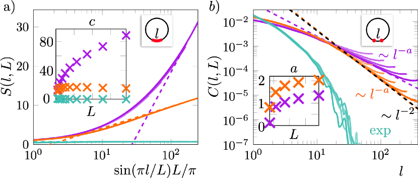
Figure 1: Further characterization of CFT ($\gamma=0.3,p=1.25$, orange), area-law ($\gamma=2,p=5$, light blue) and algebraic scaling phase ($\gamma=0.3,p=5$, purple) in terms of subsystem size dependent observables for different system sizes (different shades) up to $L=770$. a) The collapse of the entanglement entropy onto a function of the conformally invariant combination $\frac{L}{\pi}\sin\frac{\pi l}{L}$ for different $L$ breaks down in the algebraic scaling phase. Inset: $L$-dependence of the extracted effective central charge. Dashed lines: best fit under the assumption of a CFT at $L=770$. b) Emergence of algebraic scaling of the correlation function at intermediate $l$ for $L\rightarrow\infty$ in the CFT and the algebraic scaling phase. Fitting to the scaling regime yields the exponents indicated in the inset and (for $L=770$) by dashed lines in the main plot (black dashed line $\sim l^{-2}$ for comparison).

Applying the same procedure in the long-range hopping regime (purple curves in Fig. 1 and Fig. 2 in the main text) reveals a breaking of this behavior in three ways: (i) $S(l,L)$ and $C(l,L)$ do not collapse onto a function of the scale-invariant combination $\frac{L}{\pi}\sin{\frac{\pi l}{L}}$, (ii) the extracted effective central charge does not approach a finite value for for $L\to\infty$ (see Fig. 3a in the main text), indicating algebraic scaling of the entanglement entropy, and (iii) the correlation function $C(l,L)$ decays algebraically, but slower than $l^{-2}$ or $L^{-2}$. To extract the critical point, where the algebraic scaling sets in, and the exponents for both $S$ and $C$ in this regime, we use an ansatz to capture both conformal scaling and algebraic scaling, and finite size effects

$$S(L/2,L)=BL^{b}+\frac{c}{3}\log\frac{L}{\pi}+s_{0},\quad C(L/2,L)=\frac{1}{AL^{a}+DL}.$$ (9)

Fitting $B,b,c,s_{0},A,a$ and $D$ to the numerical data is sensitive to the phase transition. Especially the exponents $a$ and $b$ can be extracted quantitatively, signalling the algebraic scaling phase by $a<2$ and $b>0$ (cf. Fig. 1d,e in the main text). Comparing the exponents extracted in this way to $S(l,L)\sim l^{b}$ and $C(l,L)\sim l^{-a}$ in a scaling regime at intermediate $l$ shows good agreement (cf. Fig. 1).

IV Scaling form of long-range Hamiltonian

If the long-range hopping Hamiltonian shown in Eq. (3c) of the main text is relevant in the RG sense, we may assume a large parameter $\Delta$ and hence a pinning of $\hat{\theta}_{x}$ to a constant. Expanding around this constant (that we set to $0$ for convenience) yields to leading order and up to an additive constant

$$\hat{H}_{\text{lr}}\simeq-i\Delta\int_{x,|y|>1}|y|^{-2p}\left(\hat{\theta}_{x}-\hat{\theta}_{y}\right)^{2}.$$ (10)

Applying the Fourier transformation yields

$$\hat{H}_{\text{lr}}\simeq-8i\Delta\int_{q}\hat{\theta}_{-q}\hat{\theta}_{q}\int_{1}^{\infty}dy\frac{\sin^{2}\frac{qy}{2}}{y^{2p}}.$$ (11)

The canonical scaling dimension is then extracted from the integral

$$\int_{1}^{\infty}dy\frac{\sin^{2}\frac{qy}{2}}{y^{2p}}=|q|^{2p-1}\int_{q}^{\infty}ds\frac{\sin^{2}\frac{s}{2}}{s^{2p}}.$$ (12)

For $1<p<3/2$, taking limit $q\to 0$ yields a convergent dimensionless integral $I_{p}\equiv\int_{0}^{\infty}ds\sin^{2}(s/2)s^{-2p}>0$, such that the momentum dependence is entirely in the prefactor of the integral, and we find

$$\hat{H}_{\text{lr}}\simeq-i\Delta_{p}\int_{q}|q|^{2p-1}\hat{\theta}_{-q}\hat{\theta}_{q},$$ (13)

with $\Delta_{p}=8\Delta I_{p}>0$. Since $2p-1<2$, this is more relevant than the term $\sim q^{2}\hat{\theta}_{-q}\hat{\theta}_{q}$ from the short-range Hamiltonian (Eq. (3a) in the main text), such that we drop the latter. The fact that $\hat{H}_{\text{lr}}$ and the non-linearity in $\hat{H}_{\text{sr}}$ do not commute implies that only one of the two (in this case $\hat{H}_{\text{lr}}$) can be relevant. Together, we find the effective Hamiltonian (8) in the main text.

Conversely, if $p>3/2$, the integral $I_{p}$ is divergent and has to be regularized by re-inserting $q$ as a cutoff. The divergence of the integral precisely cancels the $p$-dependence of the prefactor, and we obtain $\sim q^{2}\hat{\theta}_{-q}\hat{\theta}_{q}$ from the long-range term, which renormalizes the parameters of the short-range Hamiltonian.

V Correlation functions

Here, we evaluate the $\hat{\phi}\hat{\phi}$ correlation function in the dark state $|\psi_{D}\rangle$ of the linearized replica Hamiltonian in the long-range regime

$$\hat{H}_{\text{eff}}=\frac{1}{2\pi}\int_{q}\left\{-i\Delta_{p}|q|^{2p-1}\hat{\theta}_{-q}\hat{\theta}_{q}+\eta q^{2}\hat{\phi}_{-q}\hat{\phi}_{q}\right\},$$ (14)

where we assume $1<p<3/2$. We represent this in terms of bosonic operators $\hat{b}_{q},\hat{b}_{q}^{\dagger}$ with $[\hat{b}_{p},\hat{b}_{q}^{\dagger}]=\delta_{p,q}$ and find

$$\hat{H}_{\text{eff}} =\int_{q}\left(\begin{array}[]{cc}\hat{b}_{q}^{\dagger}&\hat{b}_{-q}\end{array}\right)M_{q}\left(\begin{array}[]{c}\hat{b}_{q}\\ \hat{b}_{-q}^{\dagger}\end{array}\right),$$ (15d)

$$M_{q} =\frac{|q|}{4}\left(\begin{array}[]{cc}\eta+i\Delta_{p}|q|^{2p-3}&\eta-i\Delta_{p}|q|^{2p-3}\\ \eta-i\Delta_{p}|q|^{2p-3}&\eta+i\Delta_{p}|q|^{2p-3}\end{array}\right).$$ (15g)

By a Bogoliubov transformation

$$\left(\begin{array}[]{c}\hat{b}_{q}\\ \hat{b}^{\dagger}_{-q}\end{array}\right)=\left(\begin{array}[]{cc}\alpha^{*}_{-q}&-\beta_{q}\\ -\beta^{*}_{-q}&\alpha_{q}\end{array}\right)\left(\begin{array}[]{c}\hat{c}_{q}\\ \hat{c}^{\dagger}_{-q}\end{array}\right),$$ (16)

with $|\alpha_{q}|^{2}-|\beta_{q}|^{2}=1$, we bring the Hamiltonian into a tri-diagonal form in terms of the bosonic operators $\hat{c}_{q},\hat{c}_{q}^{\dagger}$,

$$\hat{H}=\epsilon_{q}\left(\hat{c}_{q}^{\dagger}\hat{c}_{q}+\hat{c}_{-q}\hat{c}_{-q}^{\dagger}\right)+\eta_{q}\hat{c}_{q}\hat{c}_{-q},$$ (17)

with $\mathop{\mathrm{Im}}\epsilon_{q}<0$, such that the excitations in the basis of $\hat{c}_{q},\hat{c}_{q}^{\dagger}$ decay exponentially in time. The term proportional to $\eta_{q}$ ensures that the system cannot be frozen in a different state. For that reason, we identify $\ket{\psi_{D}}$, defined by $\hat{c}_{q}\ket{\psi_{D}}=0$ as the dark state of the non-Hermitian Hamiltonian in the relative replica coordinate, and hence the state that determines the correlation functions in the stationary limit $t\rightarrow\infty$. The tridiagonal form demands

$$\alpha_{q}=-\beta_{q}=\frac{1}{2}\left(\frac{i\Delta_{p}}{\eta}\right)^{1/4}|q|^{p/2-3/4}+\mathcal{O}(q^{0}).$$ (18)

Higher orders in $q$ ensure the validity of the Bogoliubov transformation. In terms of the Luttinger liquid operators, we find

$$\bra{\psi_{D}}\hat{\phi}_{-q}\hat{\phi}_{q}\ket{\psi_{D}} =\frac{\pi}{2|q|}\left[1+2|\beta_{q}|^{2}-\alpha_{q}\beta_{q}^{*}-\beta_{q}\alpha_{q}^{*}\right]$$

$$=\frac{3\pi}{2}\sqrt{\frac{\Delta_{p}}{|\eta|}}|q|^{p-5/2}+\mathcal{O}(|q|^{-1}).$$ (19)

By a Fourier-transformation, we find the scaling $\langle\hat{\phi}_{x+l}\hat{\phi}_{x}\rangle\sim l^{3/2-p}$ from the main text (Eqs. (9),(10)).

VI First order renormalization group equations

We briefly review the first order perturbative renormalization group (RG) approach for sine-Gordon type models to motivate the form of the RG equations Eqs. (6)-(8) in the main text. We display the steps for the first order correction to the Hamiltonian induced by $\hat{H}_{\text{lr}}$. Canonical power counting for the terms in this Hamiltonian yields $[\Delta]=3-2p$ ($3$ counting two space integrals, one time integral). The first order RG correction is obtained from decomposing the fields $\hat{\theta}_{x}=\hat{\theta}_{x}^{<}+\hat{\theta}_{x}^{>}$ into fast, short distance modes $\hat{\theta}_{x}^{<}=\int_{\Lambda e^{-s}<|k|<\Lambda}e^{ikx}\hat{\theta}_{x}$ and slow, long distance modes $\hat{\theta}_{x}^{>}=\int_{|k|<\Lambda e^{-s}}e^{ikx}\hat{\theta}_{x}$. Here $\Lambda=\pi/a$ is the short-distance cutoff with the lattice spacing $a=1$.

The first order correction to the Hamiltonian $\Delta\hat{H}_{\text{lr}}$ is then obtained by taking the average with respect to short distance modes, assuming they are in the dark state of the quadratic part of $H_{\text{eff}}$. The cosine renormalizes multiplicatively

$$\langle\cos\left[\sqrt{2}(\hat{\theta}_{x}-\hat{\theta}_{y})\right]\rangle_{<}=\cos\left[\sqrt{2}(\hat{\theta}_{x}^{>}-\hat{\theta}_{y}^{>})\right]e^{-\langle(\hat{\theta}_{x}^{<}-\hat{\theta}_{y}^{<})^{2}\rangle_{<}}$$

$$=\cos\left[\sqrt{2}(\hat{\theta}_{x}^{>}-\hat{\theta}_{y}^{>})\right]e^{-2\langle(\hat{\theta}_{x}^{<})^{2}\rangle_{<}}(\underbrace{1}_{(\text{i})}+\underbrace{e^{2\langle\hat{\theta}_{x}^{<}\hat{\theta}_{y}^{<}\rangle_{<}}-1}_{(\text{ii})}).$$ (20)

Here $\langle...\rangle_{<}$ denotes the average with respect to the dark state $|\psi_{D}^{<}\rangle=\otimes_{\Lambda e^{-s}<|k|<\Lambda}|\psi_{D}^{k}\rangle$, where $|\psi_{D}^{k}\rangle$ is the $k$-momentum dark state of the quadratic part of $H_{\text{eff}}$. The first term (i) in Eq. (20) then represents the conventional renormalization of a $\cos$-nonlinearity, which one would obtain also for purely local terms. The second term (ii), however, is characteristic for the long-range Hamiltonian with two-different arguments $x,y$. Since both $\hat{\theta}_{x}^{<},\hat{\theta}_{y}^{<}$ are short distance modes, the average is only non-zero if $x\approx y$. We can therefore expand $y$ around $x$, and we approximate the short distance terms by their leading order contribution $y\approx x+a$. Besides being linear in $\Delta$, this term is then of the same form as the common second order perturbative correction in the conventional, local sine-Gordon model. This yields

$$\langle\cos\left[\sqrt{2}(\hat{\theta}_{x}-\hat{\theta}_{y})\right]\rangle_{<}\approx \Big{\{}e^{-\eta s}\cos\left[\sqrt{2}(\hat{\theta}_{x}^{>}-\hat{\theta}_{y}^{>})\right]$$

$$-\delta(|y-x|-a)(a\partial_{x}\hat{\theta}_{x}^{>})^{2}F_{a}\Big{\}}.$$ (21)

where $F_{a}=e^{-\eta s}(e^{2\langle\hat{\theta}_{x}^{<}\hat{\theta}_{x+a}^{<}\rangle_{<}}-1)$. Together with the canonical power counting this yields the perturbative flow equations

$$\partial_{s}\Delta =(3-2p-\eta)\Delta,$$ (22)

$$\partial_{s}\eta^{-1} =\Delta F_{a}.$$ (23)

Assuming a negligible dependence of $F_{a}$ on $s$ and rescaling $\Delta\rightarrow\Delta F_{a}$ yields the RG equations (6),(7) from the main text.