Dynamics of spectral correlations in the entanglement Hamiltonian of the Aubry-André-Harper model

Abstract

We numerically study the evolution of spectral correlations in the entanglement Hamiltonian (EH) of non-interacting fermions in the Aubry-André-Harper (AAH) model. We analyze the time evolution of the EH spectrum in a nonequilibrium setting by studying several quantities: spectral distribution, level statistics, entanglement entropy, and spectral form factor (SFF) in the context of the delocalization-localization transition in the AAH model. It is observed that the SFF of the entanglement spectrum in the delocalized phase and at the phase-transition point evolves in three time intervals. We make a systematic study of the emergence of these three timescales for various initial states and find that the number of time intervals remains three unless the Hamiltonian is tuned in the localized phase or when the initial state is maximally entangled, when there is a featureless time evolution. We find a broad direct correlation between the entanglement entropy and the length of the ramp of the SFF. We also find that in the delocalized phase the spectral correlations are stronger in the center of the spectrum and grow progressively weaker as more and more of the spectrum is considered.

I INTRODUCTION

The study of chaos in many-body quantum systems from a dynamical viewpoint is of great current interest [1, 2, 3, 4, 5, 6, 7, 8, 9, 10, 11]. In the traditional approach which has mainly focused on short-range correlations in the spectrum, level statistics, and universal spectral properties through random matrix theory (RMT) [12, 13, 14] have been popular objects of study. However other indicators of chaos such as the out-of-time order correlators (OTOC) [15, 16, 17] and the spectral form factor (SFF) [18] are also of interest. For example, they have been used to understand chaos in the Sachdev-Ye-Kitaev (SYK) model which is important in the context of blackhole physics [19, 20, 21, 22].

The spectral form factor is a useful measure for describing spectral statistics in quantum systems. It is defined as the Fourier transform of the correlation function between two levels of the spectrum [23]:

$$g(\tau)=\left\langle\sum_{i,j}e^{-i\tau\left(\lambda_{i}-\lambda_{j}\right)}\right\rangle.$$ (1)

For a chaotic quantum system, the SFF of the spectrum exhibits a “ramp” signaling the presence of universal spectral correlations whereas for an integrable system, the ramp is absent. Since it deals with the long-range correlations in the system, it presents an alternative picture from the known measures of level-statistics and hence it is being studied in a variety of models such as Floquet systems[24, 25, 26], models featuring many-body localization etc [27, 28, 29]. It has also been discussed in detail in the context of various ensembles of RMT such as the Gaussian ensembles[30, 31] or the Wishart ensembles [23, 30] and hence can serve as an indicator of quantum chaos[12].

In systems where delocalization-localization phase transitions can be observed with a change in disorder strength, entanglement entropy [32, 33] often provides valuable insights. In general, the entanglement entropy is observed to be larger in the delocalized phase due to the presence of more correlations than in the localized phase. Thus one can study this quantity together with the spectral form factor to understand the correlations of the spectrum better. One such model which exhibits a delocalization-localization transition even in one dimension is the Aubry-André-Harper model which is governed by a quasi-periodic disorder. All the single-particle states of this system are either localized or delocalized depending on the strength of the quasi-periodic disorder [34, 35, 36].

It has been seen recently that the dynamics of the spectral form factor serves as a useful probe in understanding the various stages of approach to thermalization in chaotic (non-integrable) models  [37] through the study of the correlations in the spectrum of the entanglement Hamiltonian. It has been noticed that there is a certain correspondence between the dynamics of the level repulsion, entanglement entropy  [38, 39, 40], and the development of the spectral form factor. With the aid of a variety of quantities including gap ratio and entanglement entropy, Chang et al [37] were able to identify three distinct timescales, which were observed in both the chaotic and MBL phases. In the backdrop of such interesting findings in an interacting model, it is of great interest to understand how these different timescales play out within a noninteracting model.

Here in this article, we consider the AAH model in which both delocalized and localized phases are possible depending on the strength of the disorder. It is a quadratic system with the integrability weakly broken by the disorder. We study the development of correlations in the entanglement Hamiltonian spectrum of the AAH model through quench dynamics in its different phases. Tracking the evolution of various quantities such as the gap ratio, Renyi entropies, and spectral density together with the SFF, we find the presence of three distinct timescales in both the delocalized phase and at the critical point, while is predictably flat in the localized phase. We also compare the SFF with the evolution of the higher-order gap ratios and find correspondence between both the measures. From the spectrum resolved study of the SFF, we find that the correlations in the delocalized phase are dominant more at the center of the spectrum. However, at the critical point the correlations are uniformly spread out throughout the spectrum. A systematic study of the dynamics starting from a variety of initial states allows us to conclude that the length of the ramp (in the units of $\tau$) in the SFF is strongly correlated with the magnitude of the entanglement entropy.

The paper is organized as follows. In Section II, the model Hamiltonian, spectral form factor, and the entanglement Hamiltonian are briefly introduced. The nonequilibrium dynamics of the entanglement Hamiltonian is discussed in Section III for various initial states: non-entangled and entangled. This section comprises six subsections. In Subsections III.1–III.5 the nonequilibrium dynamics for a non-entangled initial product state is studied by computing various quantities such as the gap ratio, entanglement entropy, and spectral form factor. Also, we look into the (sub)system-size dependences of these quantities. In Subsection III.6 we consider entangled initial states and study the dynamics of the corresponding EH spectrum. Then we conclude in Section IV.

II Model and Methods

II.1 Hamiltonian

We consider the AAH model given by the Hamiltonian [34, 35] :

$$H=-t\sum_{i}(c_{i}^{\dagger}c_{i+1}+H.c.)+\sum_{i}2\lambda\cos(2\pi ib+\theta_{p})c_{i}^{\dagger}c_{i}.$$ (2)

Here $c^{\dagger}_{i}$ $(c_{i})$ is the creation (annihilation) operator on site $i$. The first term describes the nearest-neighbor hopping along the chain where $t$ is the hopping parameter which we set to unity. The second term describes the quasi-periodic on-site energy where the strength of the quasi-periodic potential is $\lambda$, the quasi-periodicity parameter ‘$b$’ is taken to be an irrational number and $\theta_{p}$ is an arbitrary global phase chosen randomly from a uniform distribution in the range $[0,2\pi]$. The total number of sites is $N$ and periodic boundary conditions are assumed. As is well-known [41], all the energy eigenstates are delocalized when $\lambda<1$, and all the energy eigenstates are localized when $\lambda>1$. $\lambda=1$ is the critical point where all the eigenstates are multifractal[42]. At $\lambda=1$, the AAH model in position space maps to itself in momentum space which makes the model self-dual [34, 43]. This is observed whenever the quasiperiodicity parameter is chosen to be an irrational number. In this article, following convention, we set $b$ to be the golden mean $(\sqrt{5}-1)/2$.

II.2 Spectral form factor

The spectral form factor is used to understand the correlations present in a spectrum. Given a spectrum of $N$ eigenvalues, we consider the eigenvalue density:

$$\nu(\lambda)=\sum_{i=1}^{N}\delta(\lambda-\lambda_{i}).$$ (3)

Defining the Fourier transform of the eigenvalue density as:

$$Z(\tau)=\sum_{i=1}^{N}e^{-i\tau\lambda_{i}},$$ (4)

the spectral form factor is conveniently expressed in terms of $Z(\tau)$ as:

$$g(\tau)=\left\langle Z(\tau)Z^{*}(\tau)\right\rangle=\left\langle\sum_{i,j=1}^{N}e^{-i\tau\left(\lambda_{i}-\lambda_{j}\right)}\right\rangle,$$ (5)

where the average is taken over an ensemble in order to remove non-universal fluctuations in $g(\tau)$ (and $g_{c}(\tau)$), since it is not a self-averaging quantity  [44, 45]. In our work, we average our data over a set of values of the random phase $\theta_{p}$, as described in the previous subsection. The spectral form factor exhibits a typical structure corresponding to universal spectral correlations in the system. Starting at $N^{2}$ at $\tau=0$ it starts to decrease until it reaches a minimum, after which it shows a strictly linear growth called the “ramp” which is a signature of the presence of long-range correlations in the system. The curve then becomes constant at long times (at Heisenberg time $\tau_{H}$ defined as $2\pi$ times the inverse of the mean level spacing), reaching its ‘plateau’ value [46]: $\lim_{\tau\rightarrow\infty}g(\tau)=N$.

Another quantity of interest is the connected spectral form factor (CSFF)

$$g_{c}(\tau)=\left\langle Z(\tau)Z^{*}(\tau)\right\rangle-\left\langle Z(\tau)\right\rangle\left\langle Z^{*}(\tau)\right\rangle,$$ (6)

which is obtained by deducting the disconnected part from $g(\tau)$. The disconnected part which is non-universal  [23] is active primarily in the smaller $\tau$ regime, and leads to a reduction in the size of the ramp seen in $g(\tau)$. $g_{c}(\tau)$ explicitly removes the non-universal disconnected part, and exhibits a longer ramp for the timescale that corresponds to energy differences that lie in the universal regime.

II.3 Entanglement Hamiltonian and correlation matrix

We consider non-interacting spinless fermions at half-filling in the AAH model. To calculate the entanglement Hamiltonian  [47, 48, 49], one can divide the system into two contiguous parts, one with $N_{A}$ number of sites and the other with $N_{B}=N-N_{A}$ sites where $N$ is the total number of sites. Given the density matrix $\rho$ the reduced density matrix can be calculated as $\rho_{A}=Tr_{B}(\rho)$. Using the reduced density matrix, the von Neumann entropy of the subsystem can be calculated as $S_{A}=-Tr\left(\rho_{A}\log\rho_{A}\right)$. But for a single Slater determinant many-body state such as for free fermions, using Wick’s theorem we can write

$$\rho_{A}=\frac{e^{-H_{A}}}{Z},$$ (7)

where $H_{A}=\sum_{ij}^{N_{A}}H_{ij}^{A}c_{i}^{\dagger}c_{j}$ [47] is called the entanglement Hamiltonian, and $Z$ satisfies the condition Tr$(\rho_{A})=1$. The correlation matrix for the chosen subsystem $A$ is given as: $C_{ij}=\left\langle c_{i}^{\dagger}c_{j}\right\rangle$ where $i,j=1,2......N_{A}$. The information held in $\rho_{A}$ of size $2^{N_{A}}\times 2^{N_{A}}$ can be captured in terms of the correlation matrix $C$ of size $N_{A}\times N_{A}$ [48]. This subsystem correlation matrix is related to the entanglement Hamiltonian as

$$H_{A}=\ln\frac{1-C}{C}.$$ (8)

Thus, we can find the eigenvalues of the entanglement Hamiltonian from the eigenvalues of the correlation matrix. In the present work, we will study the spectral form factor of the entanglement Hamiltonian. While it is also meaningful to study the spectral correlations of the reduced density matrix of the subsystem  [37, 23], it is easier to consider the entanglement Hamiltonian directly due to its intimate relationship with the reduced density matrix (see Eq. 7).

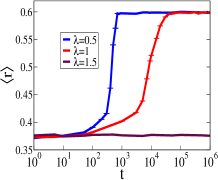
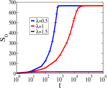
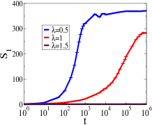
(a)  (b) (c)  (d)

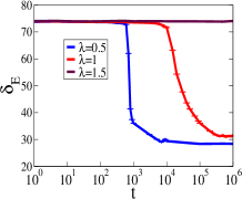
Figure 1: Spectral properties of the EH in different phases under time evolution. Here $\lambda=0.5,1,1.5$ signify the delocalized phase, phase-transition point and the localized phase respectively. Time evolution of (a) Nearest-neighbour spacing ratio $\left\langle r\right\rangle$, (b) Zeroth-order Renyi entropy $S_{0}$, (c) von Neumann entropy $S_{1}$ and (d) Entanglement Bandwidth $\delta_{E}$. Here the system size is $N=1920$ and subsystem size is $N_{A}=N/2$. The average has been taken over $100$ random values of $\theta_{p}$.

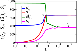
Figure 2: Scaled gap ratio $\left\langle r\right\rangle_{s}(=\eta_{1}\left\langle r\right\rangle)$ and zeroth order Renyi entropy $S_{0}$ saturating at time $t_{1}$ while scaled entanglement bandwidth $(\delta_{E})_{s}(=\eta_{2}\delta_{E})$ and von Neumann entropy $S_{1}$ saturating at time $t_{2}$. The scaling factors are $\eta_{1}=1108.0$ and $\eta_{2}=12.9533$ in the delocalized phase ($\lambda=0.5$). The system size is $N=1920$ and $N_{A}=N/2$. The average has been taken over $100$ random values of $\theta_{p}$.

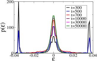
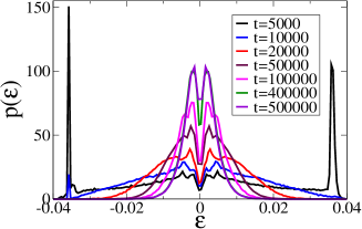
(a)    (b)    (c)

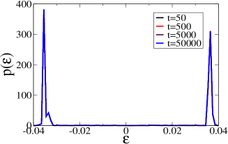
Figure 3: Time evolution of spectral density of EH (scaled with subsystem size $N_{A}$) in different phases. (a) $\lambda=0.5$: delocalized phase, (b) $\lambda=1$: phase transition point and (c) $\lambda=1.5$: localized phase. Here the system size is $N=1920$ and $N_{A}=N/2$. The average has been taken over $100$ random values of $\theta_{p}$.

III Nonequilibrium dynamics

Here we intend to understand the dynamical evolution of the spectral correlations of the entanglement Hamiltonian in different many-body phases of the AAH model. The dynamics are studied in a nonequilibrium setting starting from the initial product state $\ket{\Phi_{0}}=\prod_{i=1}^{N/2}c^{\dagger}_{2i}\ket{0}$, where $N$ is an even number. The unitary time evolution of the state is represented as

$$\ket{\Phi(t)}=e^{-iHt}\ket{\Phi_{0}}.$$ (9)

The time-dependent correlation matrix is then given by

$$C_{ij}(t)=\bra{\Phi(t)}c^{\dagger}_{i}c_{j}\ket{\Phi(t)}=\bra{\Phi_{0}}c^{\dagger}_{i}(t)c_{j}(t)\ket{\Phi_{0}},$$ (10)

where the time evolution of the operator $c_{i}(t)$ is obtained in the Heisenberg picture [48]. Thus the full time-dependent correlation matrix in the Heisenberg picture is given as

$$C(t)=e^{iHt}C(0)e^{-iHt},$$ (11)

where $C(0)$ contains the initial correlations [50]. We then obtain the correlation matrix and hence the time-dependent entanglement Hamiltonian for the choosen subsystem using Eq. 8. We stick to this non-entangled initial product state except in Subsection III.6 where we study the dynamics of initially entangled states. Our non-equilibrium setting is similar to studying a global quench in the hopping model. Using Eq. (8), one can find the time-dependent entanglement Hamiltonian, whose eigenvalues are used to study the dynamics of a number of useful quantities such as the gap ratio, Renyi entropies, and spectral form factor.

III.1 Gap ratio and Renyi entropy

The gap ratio [51] is defined as

$$r_{k}=\frac{min(s_{k},s_{k+1})}{max(s_{k},s_{k+1})},$$ (12)

where $s_{k}=e_{k}-e_{k-1}$ and $e_{k}$’s are the eigenvalues arranged in ascending order. The mean gap ratio $\left\langle r\right\rangle$ is calculated by averaging $r_{k}$ over the energy spectrum. In Fig. 1(a), $\langle r\rangle$ starts from a Poisson-like value ($\approx 0.386$). It evolves with time in a manner consistent with growing nearest neighbour correlations until it reaches the Gaussian unitary ensemble (GUE) value ($\approx 0.599$ [51]). The dynamics of higher-order gap ratios involving gaps between more than nearest energy levels is also interesting and will be discussed later (see Subsection III.4). The time at which the first order gap ratio hits its saturating value is denoted by $t_{1}$ and hence the first timescale is defined by $t<t_{1}$.

The $\alpha$^th order time-dependent Renyi entropy in terms of the eigenvalues $\lambda_{k}$’s of the subsystem correlation matrix $C(t)$ is given as [52]:

$$S_{\alpha}(t)=\frac{1}{1-\alpha}\sum\limits_{k=1}^{N_{A}}\ln\big{[}(1-\lambda_{k}(t))^{\alpha}+(\lambda_{k}(t))^{\alpha}\big{]},$$ (13)

where $\alpha$ is the order of the Renyi entropy. The zeroth order Renyi entropy $S_{0}$, by definition determines the number of non-zero eigenvalues or the rank of the reduced density matrix. The first order Renyi entropy also called the von Neumann entropy can be defined as $S_{1}=\lim\limits_{\alpha\rightarrow 1}S_{\alpha}$ which is given by:

$$S_{1}=-\sum\limits_{k=1}^{N_{A}}\big{[}\lambda_{k}(t)\ln(\lambda_{k}(t))+(1-\lambda_{k}(t))\ln((1-\lambda_{k}(t))\big{]}.$$ (14)

The above expression can also be derived via the relation in Eqn. 8 [49]. For the initial product state as considered here $S_{\alpha}=0$ at $t=0$, but $S_{\alpha}(t)>0$ otherwise. It turns out that $S_{0}$ also hits saturation along with the first-order gap ratio around $t_{1}$. We have observed that only when the correlation matrix is obtained from a product state, $S_{0}$ saturates at time $t_{1}$. In all other cases, (see Subsection III.6) $S_{0}$ remains saturated for times $t<t_{1}$ also. We are able to identify a second timescale where the first order gap ratio (and $S_{0}$ as shown in Fig. 1(b)) is saturated whereas $S_{1}$ keeps on increasing. At time $t_{2}$, $S_{1}$ also saturates [see Fig. 1(c)], thus the second timescale is defined by the interval $t_{1}<t<t_{2}$ [53]. We are also able to identify a third timescale which is marked by $t>t_{2}$.

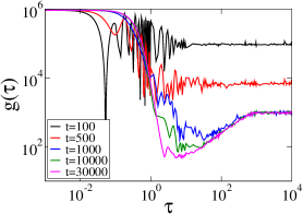
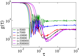
(a)    (b)    (c)

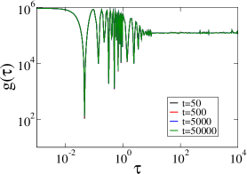
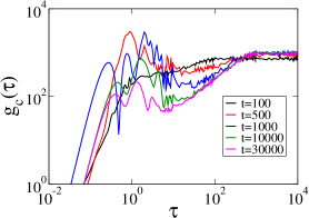
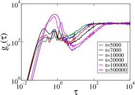
(d)    (e)    (f)

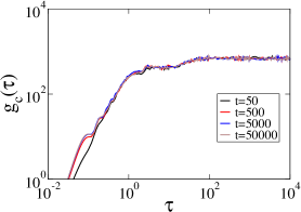
Figure 4: Time evolution of spectral form factor. Here plots (a), (b) and (c) show evolution of $g(\tau)$ (SFF) and plots (d), (e) and (f) show the evolution of connected spectral form factor $g_{c}(\tau)$ corresponding to $\lambda=0.5,1$ and $1.5$ respectively. The system size is $N=1920$ and $N_{A}=N/2$. The average has been taken over $500$ random values of $\theta_{p}$.

Another useful quantity that can be constructed from the entanglement spectrum is the entanglement bandwidth. It is defined as

$$\delta_{E}=E_{max}-E_{min},$$ (15)

where $E_{max}$ and $E_{min}$ are the maximum and minimum eigenvalues of the entanglement Hamiltonian. We find that for times beyond $t>t_{2}$, it is not just $S_{1}$ that saturates, but in fact the entire EH spectrum that saturates, and hence $\delta_{E}$ also saturates as shown in Fig. 1(d). Thus the onset of saturation in $\delta_{E}$ also determines the onset of the third timescale. Also from Fig. 2 it can be observed, that on scaling the nearest-neighbour gap ratio $\left\langle r\right\rangle$ [see Fig. 1(a)] by a factor $\eta_{1}$, it can be compared with the zeroth order Renyi entropy $S_{0}$ [see Fig. 1(b)] and hence it becomes apparent that they both reach saturation at time $t_{1}$. Similarly, it can be observed that the entanglement bandwidth $\delta_{E}$ can be scaled by a factor $\eta_{2}$ and at $t_{2}$ it reaches saturation together with the von Neumann entropy $S_{1}$. Since they both depend on the EH spectrum, they saturate as soon as the spectrum saturates i.e. at $t_{2}$. This can be seen in both the delocalized phase and at the critical point.

To understand the above observations better for different phases, it is useful to study the probability distribution of the eigenvalues of the entanglement Hamiltonian at different instants of time[54]. The evolution of the spectral density of EH is shown in Fig. 3 for different phases. Referring to Eq. 8 and Eq. 14 we observe that the near-zero eigenvalues of the EH contribute maximally to the entanglement entropy whereas the eigenvalues with large magnitudes barely contribute to it. As shown in Fig. 3(a) and Fig. 3(b) the initial state corresponds to large eigenvalues of the EH, and thus the entanglement entropy is also very low. As EH evolves with time the eigenvalues become smaller thus contributing more to the entanglement entropy. However, Fig. 3(c) shows that in the localized phase the distribution does not change from its initial bimodal form with the peaks remaining at large values. This implies almost no growth in entanglement entropy in the localized phase [see Fig. 1(c)].

We notice that in the delocalized phase during the first timescale ($t<t_{1}$) the spectral distribution carries the bimodal peaks and at the end of this timescale the distribution attains a single peak about zero with the bimodal structure dismantled. In the second timescale ($t_{1}<t<t_{2}$), the single peak continues to develop further and saturates on reaching the third timescale. This is also observed from Fig. 2 where at time $t_{1}$, a sharp transition can be seen in the scaled entanglement bandwidth $(\delta_{E})_{s}$, though it reaches saturation later only at time $t_{2}$. At the critical point $\lambda=1$ qualitatively the scenario remains the same as in the delocalized phase. However, one obtains bimodal peaks close to zero in the second timescale in this case instead of a single peak about zero in the delocalized phase. In the localized phase, the spectrum does not evolve with time and hence the distribution does not change. This analysis of timescales as discussed here is consistent with the analysis obtained from the other quantities studied in Fig. 1.

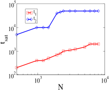
(a)  (b)

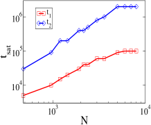
Figure 5: System size dependence of times $t_{1}$ and $t_{2}$ for the initial product state (a) $\lambda=0.5$ and (b) $\lambda=1$. In all cases $N_{A}=N/2$ and average has been taken over a range of $100-30$ random values of $\theta_{p}$ (depending on system size).

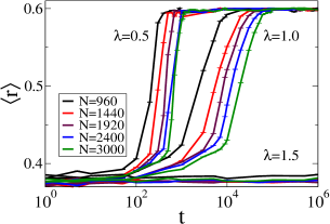
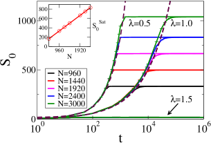
(a)   (b)   (c)

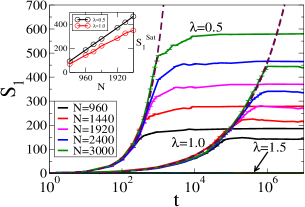
Figure 6: System size effects on (a) Gap ratio, (b) Zeroth-order Renyi Entropy and (c) von Neumann Entropy for the different phases corresponding to $\lambda=0.5,1.0,1.5$. Here the power law dependence is shown by fitting non-linear maroon curves in (b) and (c) with the expression $S_{\alpha}^{\lambda}(t)=ct^{\gamma}+d$: $S_{0}^{0.5}(t)=1.86t^{0.88}+17.20$, $S_{0}^{1}(t)=6.57t^{0.47}$, $S_{1}^{0.5}(t)=t^{0.90}$ and $S_{1}^{1}(t)=5.15t^{0.31}-17.02$. The insets in (b) and (c) show dependence of saturated magnitude of $S_{0}$ and $S_{1}$ on system size. Here the subsystem size is $N_{A}=N/2$ for all cases. The average has been taken over $100$ random values of $\theta_{p}$.

III.2 Spectral form factor

Through the above analysis based on gap ratio, the spread of the nearest-neighbor (NN) spectral correlations in the entanglement spectrum becomes clear. However, we are interested in understanding the global spread of correlations in the spectrum. Hence the spectral form factor (SFF) defined in Subsection II.2 becomes an appropriate measure for it. It is sensitive not only to long-range correlations but also to the density of states, unlike the gap ratio. Figures  4(a)–4(c) show the evolution of the SFF and Figs. 4(d)–4(f) show the evolution of the CSFF of the EH in different phases.

Here we associate the time evolution of the features of SFF with times $t_{1}$ and $t_{2}$ as discussed in the previous section. The nearest-neighbor repulsion in the spectrum develops till $t<t_{1}$. However as the spectral form factor also quantifies longer-correlations, it keeps developing between $t_{1}<t<t_{2}$. For time $t>t_{2}$ the entanglement spectrum does not evolve and consequently the SFF also becomes time-independent.

The time taken for the SFF to reach saturation in the delocalized phase is less than that at the critical point [see Figs. 4(a)–4(b)]. The short-time growth of the entanglement entropy is seen to be slower at the critical point [see Fig. 1(c)] in comparison with the delocalized phase because the eigenstates at the critical point are barely extended in nature. The length of the ramp (in units of $\tau$) is nearly the same in both cases which shows that the number of eigenvalues that exhibit universal spectral correlations is also approximately equal. Also there are initial fluctuations seen at earlier values of $\tau$ in all the cases of $g(\tau)$ which are absent in $g_{c}(\tau)$. These are non-universal and depend on the spectral density of the Entanglement Hamiltonian of the AAH model. In the localized phase, one can observe that irrespective of the time of evolution, $g(\tau)$ does not develop any ramp-like structure. For $\tau\rightarrow\infty$, it can be concluded from Eq. 5 that the only terms which will survive are those where $\lambda_{i}=\lambda_{j}$. Since the subsytem size is $N/2$ here, hence $g(\tau)=N/2$. Also as $\tau\rightarrow\infty$, the disconnected part $\left\langle Z(\tau)\right\rangle\left\langle Z^{*}(\tau)\right\rangle=0$ (see Eq. 6), which in turn implies that $g_{c}(\tau)=g(\tau)=N/2$. The same can be observed from Fig. 4. Hence the spectral form factor serves as a probe to distinguish between the different phases of the spectrum.

III.3 System and Subsystem size dependence

Starting from the initial product state, the system size and subsystem size dependences are studied here in different phases. The system size dependences on $t_{1}$ and $t_{2}$ in the delocalized phase and at the phase-transition point are shown in Fig. 5(a) and Fig. 5(b) respectively. We define $t_{1}$ as the time beyond which the (numerically determined) time derivative of the NN gap ratio i.e. $\frac{d\left\langle r\right\rangle}{dt}$ remains consistently below $10^{-5}$. Similarly, $t_{2}$ is defined as the time beyond which the time-derivative of the entanglement entropy ($\frac{dS_{1}}{dt}$) remains consistently below $10^{-5}$. For a clean system (results not shown here), we find that there is a systematic increase in the time $t_{2}$ with increasing system sizes. A similar trend is also expected in the case of disordered systems, which is unclear here from Fig. 5 on account of the high cost of the numerical probe. However, we are guaranteed that the time $t_{1}$ will not cross time $t_{2}$. This is due to the fact that the the butterfly velocity $v_{B}$ is generically larger than the entanglement velocity $v_{E}$ and hence the spectrum develops level repulsion before the von Neumann entropy reaches its saturation value.[53].

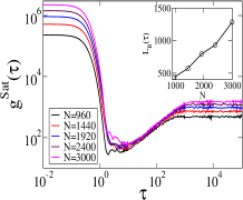
(a)  (b)

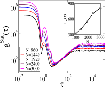
Figure 7: SFF at time $t=10^{6}$ corresponding to various system sizes for (a) the delocalized phase: $\lambda=0.5$ and (b) at the critical point : $\lambda=1.0$. Here subsystem size is $N_{A}=N/2$ in all cases. Inset shows the length of the ramp $L_{R}$ (in units of $\tau$) corresponding to various system sizes. The length of the ramp here is determined numerically by subtracting the Thouless time (local minimum of the CSFF) from the plateau time, which is taken to be the $\tau$ at which $g_{c}(\tau)$ reaches $98\%$ of its maximum value (i.e. $N_{A}$). The average has been taken over $500$ random values of $\theta_{p}$.

The system size dependences of the gap ratio, zeroth-order Renyi entropy and entanglement entropy are also discussed here [see Figs. 6(a)–6(c)]. It can be seen from Fig. 6(c), that the EE in the localized phase is independent of the system size and hence it exhibits an area-law-like behavior i.e. $S_{1}$ is constant, despite the state itself involving all the excited eigenstates as well. Also, it can be observed that the zeroth and first-order Renyi entropy at short times shows a power-law dependence on time $t$ in the delocalized phase and at the critical point i.e. $S\propto t^{\gamma}$ where $\gamma$ is some exponent which is system size independent [55]. The span of growth of entanglement entropy is larger at the critical point with smaller saturation values as compared to the delocalized phase. The EH eigenvalues in the delocalized phase have smaller magnitude than those at the phase transition point [see Figs. 3(a)–3(b)], therefore the EE tends to be larger in the delocalized phase. It can also be observed that when entropy reaches its saturation value it obeys volume law, i.e. both $S_{0}$ and $S_{1}$ at saturation increase linearly with $N$ [see insets of Figs. 6(b)–6(c)].

Since $S_{0}$ signifies the number of non-zero eigenvalues of the RDM of the subsystem ${\rho_{m}}$, and eigenvalues of EH are related to it as $\left\{E_{m}\right\}=\left\{-\log\rho_{m}\right\}$, it can be concluded that though the number of non-zero eigenvalues of the RDM is the same in both phases, their magnitudes are different as observed from $S_{1}$. In general for any $i>j$, $S_{i}\leq S_{j}$ [56]; in particular, $S_{1}$ the von Neumann entropy is a lower bound for $S_{0}$ as observed from Fig. 6(b) and Fig. 6(c).

We have seen that at long times, the system saturates to a state whose properties depend on the phase in which the Hamiltonian is tuned (see Fig. 1). Here we study the system-size dependence of the SFF of the states attained at long times. Figure 7(a) and Fig. 7(b) show the system size dependence of the SFF calculated from the states at time $t=10^{6}$ for the delocalized phase and at the phase transition point respectively. It can be observed, especially from the linear scale (see inset) that the length of the ramp ‘$L_{R}$’ (in units of $\tau$) increases as the system size becomes larger. This signifies that with a change in the system size, the number of eigenvalues that exhibit universal spectral correlations also increases which in turn leads to a longer ramp. Also, we have studied the subsystem size dependence on the length of the ramp, which is not shown here. Our main observation from this study is that for a given system size, as the subsystem size is increased (even for sizes much smaller than $\frac{N}{2}$), the length of the ramp tends to saturate, thus signaling a characteristic length of the ramp for a given system size.

III.4 Higher-order gap ratio

The nearest-neighbor level spacing ratio as defined in Eq. 12 can be generalized to the $n^{th}$ order gap ratio which examines the variations in the higher-order gaps of the spectrum. These higher-order gap ratios are focussed on larger spectral intervals and can be compared with the SFF, which is also a probe of global correlations in the spectrum. The $n^{th}$-order gap ratio is defined as:

$$r_{k}^{(n)}=\frac{min(s_{k}^{(n)},s_{k+n}^{(n)})}{max(s_{k}^{(n)},s_{k+n}^{(n)})},$$ (16)

where $s_{k}^{(n)}=e_{k}-e_{k-n}$. We study the evolution of this quantity for the dynamics starting with the initial product state, when the system is tuned in the delocalized phase and at the critical point.

Figure 8 shows the time evolution of the higher-order gap ratio for a number of different orders. In general, it can be observed that as the order ‘$n$’ increases, the time taken for the gap ratio $\left\langle r^{(n)}\right\rangle$ to saturate also increases. As discussed earlier $\left\langle r^{(1)}\right\rangle$ saturates at time $t_{1}$. In the delocalized phase, it can be seen from Fig. 8(a) that the time taken for the gap ratio of order $n=2$ to saturate is around $t=10^{3}$ at which, it can be observed [see Fig. 4(a)] that the SFF is still evolving. Tracking the higher-order gap ratios and their saturation, we observe that $\left\langle r^{(14)}\right\rangle$ reaches saturation at $t\approx 30000$ (which corresponds to time $t_{2}$), at which point the SFF is also saturated [see Fig. 4(a)]. All higher-order gap ratios beyond $n=14$, saturate at time $t_{2}$ which can also be seen from $\left\langle r^{(n)}\right\rangle$ with $n=50$ here. We conclude that the development of higher-order correlations are encapsulated in the SFF. Similarly at the critical point, from Fig. 8(b) and Fig. 4(b), all $\left\langle r^{(n)}\right\rangle$ with orders higher than $n=14$ saturate approximately at time $t_{2}$ along with the SFF. Thus there exists a correspondence between the higher-order gap ratios and SFF, both of which are measures of long-range spectral correlations.

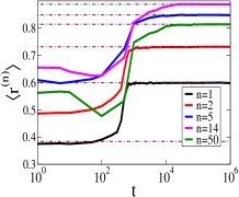
(a)  (b)

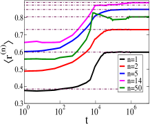
Figure 8: Time evolution of $n\textsuperscript{th}$ order gap ratio of EH spectrum for (a) $\lambda=0.5$ and (b) $\lambda=1$. The horizontal dot-dashed lines are used to show time of satuartion. Figures correspond to $N=1920$ and $N_{A}=N/2$. The average has been taken over $100$ random values of $\theta_{p}$.

III.5 Spectrum resolved SFF

Here the spectrum of the EH is divided into subsets [23](with eigenvalues arranged in ascending order) and time evolution of the SFF corresponding to each subset has been plotted in Fig. 9. This is used to understand the time evolution as well as the spread of the spectral correlations in the eigenvalues present in a particular span of the spectrum.

In Fig. 9(a), the spectrum-resolved SFF considering the bottom $1/8\textsuperscript{th}$ of the eigenvalues of the EH spectrum is plotted. Since the spectrum is symmetric about zero, the same behavior can also be observed with the top $1/8\textsuperscript{th}$ of the eigenvalues of the spectrum. The ramp here is smaller as compared to subsets of eigenvalues that lie at the center of the spectrum. For example, we see a larger ramp in Fig. 9(b) where the SFF is computed with $1/4\textsuperscript{th}$ of the total number of eigenvalues above the bottom set. We also observe an earlier dephasing in Fig. 9(a) on account of the larger magnitude of the eigenvalues involved. As one moves towards the center of the spectrum, the ramp becomes longer and dephases later. At saturation, the length of the ramp is longest for the middle of the spectrum as shown in Fig. 9(c) (where the central $1/4\textsuperscript{th}$ of the eigenvalues are used to compute the SFF). Figure 9(d) shows the evolution of the SFF considering the next $1/4\textsuperscript{th}$ of the total number of eigenvalues. Due to the symmetry of the eigenvalues on either side of the central eigenvalue, the features of the SFF at saturation in Fig. 9(b) and Fig. 9(d) are almost identical.

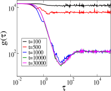
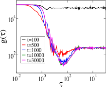
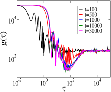
(a)  (b) (c)  (d)

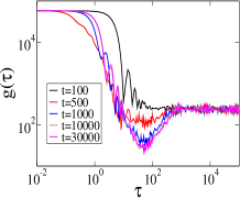
Figure 9: SFF for subset of eigenvalues (arranged in ascending order) at different time steps $t$ of the EH spectrum for $\lambda=0.5$, $N=1920$ and $N_{A}=N/2$ over $100$ realizations. Subset of eigenvalues (a) $1-120$ (bottom $1/8\textsuperscript{th}$), (b) $121-360$ ($1/4\textsuperscript{th}$ above (a)), (c) $361-600$ (central $1/4\textsuperscript{th}$) and (d) $601-840$ ($1/4\textsuperscript{th}$ above (c)).

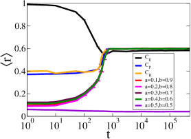
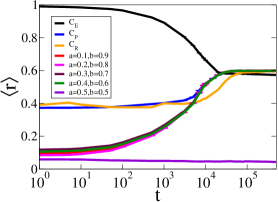
(a)    (b)    (c)

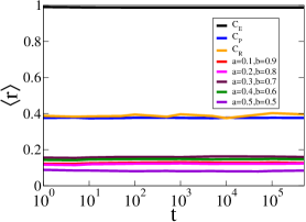
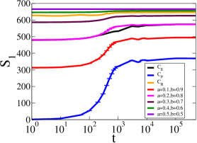
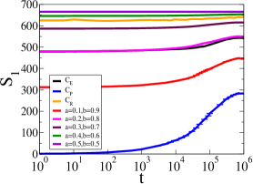
(d)    (e)    (f)

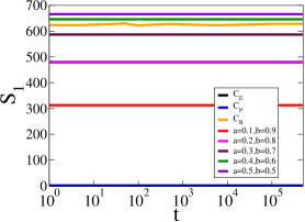
Figure 10: Evolution of the spectral properties of the EH obtained from various initial correlation matrices: $C_{E}$ matrix, $C_{P}$ matrix, $C_{R}$ matrix and $C_{S}$ matrix for $N=1920$ and $N_{A}=N/2$. Gap ratio for (a) $\lambda=0.5$, (b) $\lambda=1.0$ and (c) $\lambda=1.5$. Also von Neumann entropy for (d) $\lambda=0.5$, (e) $\lambda=1.0$ and (f) $\lambda=1.5$. The average has been taken over $100$ random values of $\theta_{p}$.

It can be concluded that in the delocalized phase, the correlations are concentrated more at the center of the spectrum and as one moves towards the edges, these correlations decrease. This happens as the contribution to entanglement come mostly from smaller magnitude eigenvalues. We have checked that at the phase-transition point $\lambda=1$, the length of the ramp at saturation corresponding to the top(or bottom) $1/8\textsuperscript{th}$ of the eigenvalues is smallest (in units of $\tau$). However, the other subsets, namely the next $1/4\textsuperscript{th}$ and the central $1/4\textsuperscript{th}$ of the eigenvalues show the same length of the ramp at saturation. Our main observation from the study of the length of the ramp at saturation is that the correlations at the critical point are more uniformly spread out than in the delocalized phase. We have also calculated the first order gap ratio $\langle r\rangle$ for various subsets of the EH spectrum. We observe that all subsets eventually reach close to the GUE value $\approx 0.599$ at nearly the same time i.e. the time taken for all the subsets to develop NN level repulsion is the same.

III.6 Dynamics of initially entangled system

So far, we have considered the dynamics of the system starting from an initial product state with a non-entangled subsystem correlation matrix. As time evolves, we have seen how entanglement tends to grow and saturate to a characteristic value at long times. In the current subsection, we will study the dynamics of the system considering a variety of initial (subsystem) correlation matrices with non-zero entanglement entropy at time $t=0$. The gap ratio of the EH related to the product state we have considered so far corresponds to the Poissonian value of $\langle r\rangle=0.38$. We now consider three different kinds of initial states whose gap ratios are different from the Poissonian value and track the evolution of these states.

Firstly, we take the correlation matrix of the full system to be a diagonal matrix whose elements are drawn from a Gaussian distribution, with the constraint that the sum of its diagonal terms is equal to the number of fermions. The corresponding correlation matrix denoted by ‘$C_{R}$’ is given by:

$$C_{R}=\xi\begin{bmatrix}c_{11}&0&0&0&\cdot\\ 0&c_{22}&0&0&\cdot\\ 0&0&c_{33}&0&\cdot\\ 0&0&0&c_{44}&\cdot\\ \cdot&\cdot&\cdot&\cdot&\cdot\\ \end{bmatrix},$$ (17)

where $c_{11},c_{22},c_{33},..$ are numbers drawn randomly from a Gaussian distribution $\mathcal{N}(0.5,0.02)$, and the normalization $\xi$ is set according to the number of fermions. For implementing the constraint, we fix $\xi$ such that the trace of the resulting matrix is equal to the number of fermions which in our case is taken to be $N/2$. The results shown here are qualitatively independent of the type of distribution from which the diagonal elements are drawn (we have checked the same for a uniform distribution $\mathcal{U}(0,1)$.)

Using the above correlation matrix, quench dynamics is studied for the AAH model. The NN gap ratio evolves starting from the Poissonian value and saturates to the GUE value at late times except in the case of the localized phase which does not show any evolution [see Figs. 10(a)–10(c)]. Here since the initial correlation matrix eigenvalues are engineered to lie close to $0.5$, the corresponding EH eigenvalues have very small magnitude, and thus it can be seen that the EE is close to the maximum entropy. Also its evolution is similar to that of the non-entangled initial product state as discussed in the previous subsections whose correlation matrix is denoted here as ‘$C_{P}$’ [see Figs. 10(d)–10(f)]. We have also checked the effect of the inclusion of small off-diagonal terms into Eq.  17. We find that the resulting time-evolved state’s spectral properties are similar to those evolving from the ‘$C_{R}$’ matrix, though the magnitude of EE becomes higher as the number of non-zero off-diagonal elements of the matrix increase.

Secondly we have considered an initial (system) correlation matrix obtained from the superposition of two DW-type pure states, $\ket{\Phi_{0}}=\prod_{i=1}^{N/2}c^{\dagger}_{2i}\ket{0}$ with probablilty amplitute $\sqrt{a}$ and $\ket{\psi_{0}}=\prod_{i=1}^{N/2}c^{\dagger}_{(2i-1)}\ket{0}$ with probabilty amplitute $\sqrt{b}$. This correlation matrix is denoted by ‘$C_{S}$’:

$$C_{S}=\begin{bmatrix}c_{11}&0&0&0&\cdot\\ 0&c_{22}&0&0&\cdot\\ 0&0&c_{33}&0&\cdot\\ 0&0&0&c_{44}&\cdot\\ \cdot&\cdot&\cdot&\cdot&\cdot\\ \end{bmatrix}.$$ (18)

Here for all odd values of ‘$i$’, $c_{ii}=b$ while for all even values of ‘$i$’, $c_{ii}=a$. Tuning the parameters $a=1$ and $b=0$, we get the initial product state denoted by ‘$C_{P}$’, for which the results have already been discussed. For $a=0.5$ and $b=0.5$, we get the maximally entangled state which does not show any evolution, and hence there is no timescale associated with it. For all other values of $a$ and $b$, the state is entangled. It can be observed from Figs. 10(a)–10(c) that the magnitude of the NN gap ratios corresponding to various values of $a$ and $b$ are initially much below the Poissonian value (i.e. 0.38). However, they also evolve with time to saturate at the GUE value except in the localized phase, where completely flat time evolution is seen. Also, it can be noted from Figs. 10(d)–10(f), that with the change in parameters the initial entanglement entropy of the subsystem increases until it reaches the value $N_{A}\ln 2$ for the maximally entangled state. As a result of the subsystem having non-zero entanglement initially, the time taken for the EE to reach saturation decreases which reduces the second timescale in both the delocalized phase and at the phase-transition point in comparison to $C_{P}$.

Next, we study another kind of initially entangled state with a tridiagonal correlation matrix denoted by ‘$C_{E}$’. The main aim here is to understand the evolution of a state which initially has nearly equally distant eigenvalues and hence shows a higher value of the NN gap ratio, i.e. whose eigenvalues are more correlated than GUE. Here the diagonal terms are determined in such a way, that they mimic the energy levels of a harmonic oscillator  [57] and the off-diagonal terms are added keeping in mind the positive semi-definite nature of the correlation matrix. The matrix corresponding to it is given by:

$$C_{E}=\begin{bmatrix}c_{11}&c_{12}&0&0&\cdot\\ c_{12}&2c_{11}&c_{23}&0&\cdot\\ 0&c_{23}&3c_{11}&c_{34}&\cdot\\ 0&0&c_{34}&4c_{11}&\cdot\\ \cdot&\cdot&\cdot&\cdot&\cdot\\ \end{bmatrix}.$$ (19)

and has nearly equidistant eigenvalues. Here the value of the term $c_{11}=\frac{2N_{P}}{N(N+1)}$, where ‘$N_{P}$’ is the number of fermions (which is equal to $N/2$ here) and ‘$N$’ is the total number of sites (i.e. the dimension of the system). The off-diagonal elements here are chosen such that for any value of ‘$i$’, $\sum_{i\neq j}c_{ij}<c_{ii}$ to satisfy the positive semi-definite nature of the matrix. We also observe that evidently, the trace of the matrix $C_{E}$ is equal to $N/2$, the number of fermions. The resulting EH of the subsystem also has nearly equally distant eigenvalues, thus the gap ratio is initially $\approx 1$. We notice from Figs. 10(a)–10(b) that it evolves with time eventually to nearly the GUE value.

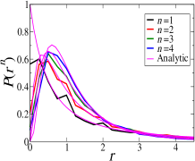
(a)  (b)

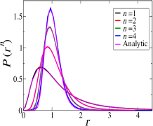
Figure 11: Distribution of $n\textsuperscript{th}$ order spacing ratios of EH spectrum for $\lambda=0.5$, $N=1920$ and $N_{A}=N/2$ with corresponding analytic curves. (a) At an early time $t=1$ and (b) at a late time $t=10^{5}$. The average has been taken over $5000$ random values of $\theta_{p}$.

It can be concluded that irrespective of the initial state, the nearest neighbor gap ratio of the system evolves and saturates to the GUE value in the delocalized phase and at the phase transition point [see Figs. 10(a)–10(b)]. However for the localized phase, the system does not show any evolution irrespective of the initial state of the system [see Fig. 10(c)]. Also, the evolution of the EE for the delocalized phase and at the critical point, are plotted in Fig. 10(d) and Fig. 10(e) respectively.

In order to get a finer understanding of the nature of the initial and final states, we also study the $n\textsuperscript{th}$ order gap ratio given by:

$$r_{i}^{(n)}=\frac{s^{(n)}_{i+n}}{s^{(n)}_{i}}.$$ (20)

Note that this definition is a little different from the higher-order gap ratio definition in Eq. 16. We have considered this variant (Eq. 20) here, since benchmark analytic results for the probability distribution of this $n\textsuperscript{th}$ order spacing ratios have been obtained for Gaussian ensembles [58] and for uncorrelated eigenvalues [59]. For the initial product state ($C_{P}$) in the delocalized phase i.e. $\lambda=0.5$, the distribution for NN spacing ratio $n=1$ as well as higher-orders $n=2,3,4$ have been plotted at the initial time, Fig. 11(a) and in the long-time limit, Fig. 11(b). The analytic distributions [58, 59] $P(r^{n})$ are found to match with our numerically determined distributions. We observe that at early times when the NN gap ratio is $\approx 0.38$, the distributions of $n\textsuperscript{th}$ order spacing ratios are also found to match with those obtained from a sequence of uncorrelated eigenvalues whereas at late times when $\left\langle r\right\rangle\approx 0.599$ the distributions match with those obtained from the spectrum of random matrices drawn from a GUE. Also in Figs. 8(a)–8(b) at saturation the average value of $r$, was found to match with the GUE values[58].

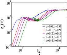
(a)  (b)

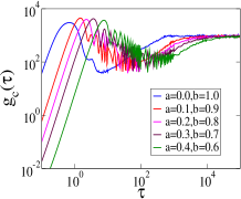
Figure 12: Connected spectral form factor (at saturation) $t=5\times 10^{5}$, considering various values of $a$ and $b$ of the correlation matrix ‘$C_{S}$’. Here (a) $\lambda=0.5$ and (b) $\lambda=1.0$ for $N=1920$ and $N_{A}=N/2$. The average has been taken over $500$ random values of $\theta_{p}$.

Similar results were observed for the higher-order spacing distributions at both early and late times in the case of the the initially entangled state obtained from the correlation matrix $C_{R}$. We have also studied the same for the case of the entangled initial state obtained from the correlation matrix $C_{S}$. We find that $P(r^{n})$ here does not match with the analytic distributions corresponding to uncorrelated eigenvalues at early times, but at late times they show distributions obtained from the spectrum of random matrices drawn from a GUE. In the case when the EH of the subsystem has nearly equally distant eigenvalues (corresponding to $C_{E}$), at early times the higher-order distributions of the gap ratios are peaked at $\approx 1$ as the eigenvalues are highly correlated. At late times only the distribution for the order $n=1$ was found to match with that proposed by Ref. 58.

The SFF-related results are next discussed for the various initially entangled subsystems described above. Figure 12(a) and Fig. 12(b) show the connected spectral form factor $g_{c}(\tau)$ at saturation (long-time limit) for different values of $a$ and $b$ for the delocalized phase and at the critical point respectively. We have determined the length of the ramp as follows. The time ($\tau$) at which the ramp starts (i.e. the Thouless time) is also a local minimum of the connected SFF which can be found by zooming in the area close to the local minimum and then determining it. For the plateau time (i.e the value of $\tau$ at which $g(\tau)$ or $g_{c}(\tau)$ saturates), we consider the time taken for $g_{c}(\tau)$ to reach $90\%$ (allowing some room for fluctuations) of its saturation value (i.e. $\lim_{\tau\rightarrow\infty}g_{c}(\tau)=N_{A}$). The length of the ramp can be found by deducting the Thouless time from the plateau time.

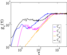
(a)  (b)

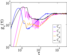
Figure 13: Connected spectral form factor (at saturation) $t=5\times 10^{5}$, for various initial correlation matrices: $C_{E}$ matrix, $C_{P}$ matrix, $C_{R}$ matrix and $C_{S}$ matrix (here $a=0.2$, $b=0.8$) for $N=1920$ and $N_{A}=N/2$. Here (a) $\lambda=0.5$ and (b) $\lambda=1.0$ for $N=1920$ and $N_{A}=N/2$. The average has been taken over $500$ random values of $\theta_{p}$.

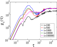
(a)  (b)

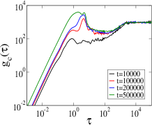
Figure 14: Evolution of connected spectral form factor obtained from the spectrum of EH corresponding to the $C_{E}$ matrix. (a)$\lambda=0.5$ and (b)$\lambda=1.0$. Here system size $N=1920$ and $N_{A}=N/2$. The average has been taken over $500$ random values of $\theta_{p}$.

As one goes from the product state to the maximally entangled state, the magnitude of EE increases at saturation [see Figs. 10(a)–10(b)]. This is due to decreasing magnitude of the eigenvalues of the EH. Since the smaller the magnitude of the eigenvalues, the larger will be the value of $\tau$ at which their difference dephases, the length (in units of $\tau$) of the ramp will become longer with the increasing value of EE. The same is true when we compare the connected spectral form factor in the long-time limit for the various correlation matrices, in the delocalized and critical phases which are shown in Figs. 13(a) and Fig. 13(b) respectively. It can be concluded that there exists a correspondence between the magnitude of EE and the length of the ramp (in units of $\tau$) which is not apparent through the NN gap ratio. A systematic comparison of the states attained by the system starting from various initial states is useful. During the first timescale, the length of the ramp is always longer corresponding to a higher EE, irrespective of the magnitude of the NN gap ratio. However if EEs are comparable (eg compare $C_{E}$ and $C_{S}$ with $a=0.2$ and $b=0.8$), the NN gap ratio seems to come into play. We observe that the length of the ramp corresponding to a higher NN gap ratio is longer. Also in the maximally entangled case i.e. when $a=0.5$ and $b=0.5$, we find both numerically and analytically that $g(\tau)=N_{A}^{2}$, while $g_{c}(\tau)=0$, on account of all the EH eigenvalues being $\approx 0$. In the second timescale since the NN gap ratios have already saturated, we see a clear monotonic relationship between the length of the ramp and the EE.

When the initial state corresponds to the $C_{E}$ matrix, we see a distinct feature that is observable from Figs. 14(a)–14(b), which present the evolution of $g_{c}(\tau)$ in the delocalized phase and at the critical point respectively. Here due to the presence of correlations in the spectrum initially, the ramp structure is observed even at early times. This however also evolves with time and saturates for time $t>t_{2}$ i.e. when von-Neumann entropy saturates. The change in the length of the ramp as time evolves is not very clear here and requires further investigation. In particular, it would be interesting to study if the presence of initial higher-order correlations in the system is the reason for this anomalous behavior. In the localized phase, the ramp does not evolve, independent of the initial spectral correlations.

IV Conclusion

We present a study of the non-equilibrium dynamics of the entanglement spectrum of a disordered integrable system, namely the Aubry-André-Harper model which hosts a delocalization-localization transition. For a system of non-interacting fermions in 1-D, we numerically explore the presence and the development of spectral correlations in the entanglement Hamiltonian spectrum. We explore the time evolution of the spectral form factor which is a measure of long range correlations, along with other quantities such as the gap ratio and the Renyi entropies for various initial (subsystem) correlation matrices. The spectral form factor exhibits a characteristic ‘ramp’ structure whose length is intimately connected to the spectral correlations.

We have analyzed various aspects of the EH spectrum when an initial state of the system is density-wave (DW) type and is evolved under the Hamiltonian. One can see the presence of three distinct timescales in the delocalized phase and at the critical point. We identify the time $t_{1}$ at which the NN gap ratio saturates along with the zeroth-order Renyi entropy $S_{0}$ and the time $t_{2}$ at which both the von Neumann entropy $S_{1}$ and entanglement bandwidth $\delta_{E}$ saturate. The three timescales are defined by $t<t_{1}$, $t_{1}<t<t_{2}$ and $t>t_{2}$. In addition, we also find signatures of the timescales from the evolution of the spectral density of the EH. We observe from the SFF that the length of the ramp (in units of $\tau$) is nearly the same in the delocalized phase and at the critical point which signifies that the number of eigenvalues that exhibit universal spectral correlations are approximately equal for both. However, in the localized phase, the time evolution is seen to be completely flat, which is characteristic of localization.

Also, a comparison between zeroth and first-order Renyi entropies shows that at saturation though the number of non-zero eigenvalues are the same for both the delocalized phase and at the critical point their magnitudes are significantly different. The length of the ramp of the SFF is also observed to decrease with the system size. We also study the time evolution of the higher-order gap ratio. It is observed that the time taken for $n^{th}$ order gap ratio to saturate increases initially with the order ‘$n$’ till a certain order, after which all higher orders saturate at the same time ‘$t$’ at which the SFF also saturates. A spectrum-resolved study of the spread of correlations reveals that in the delocalized phase, the spectrum becomes more correlated as we move towards the center from the edges while at the phase transition point they are more evenly spread out through the spectrum.

We also study the dynamics starting from a variety of initial states. For all possible initial states, one can see that the gap ratio eventually saturates approximately to its GUE value in the delocalized phase and at the phase-transition point. The three timescales exist for all these states, however, when the entanglement in the initial state is high, the second timescale becomes smaller. It is also observed that generically the length of the ramp (in units of $\tau$) is greater when the corresponding entanglement entropy has a higher magnitude. However, there are some exceptions to this trend when the gap ratio also seems to play a role.

In our study, we are able to link the long-range spectral correlations quantified by the spectral form factor to various physically relevant observables in a disordered integrable model by studying the quench dynamics of the system in different phases. As a future possibility, one can also study interacting versions of this and other allied models [60]. Another interesting direction would be to probe higher moments of the spectral form factor. The SFF remains to be explored in several contexts where the spectral correlations of the entanglement spectrum are important. An inexhaustive list of systems where this quantity may potentially find application includes periodically driven systems [61, 62], open quantum systems [63, 64], non-Hermitian [65, 66] and topological [67, 68] systems.