Understanding and Improvement of Adversarial Training for Network Embedding from an Optimization Perspective

Abstract.

Network Embedding aims to learn a function mapping the nodes to Euclidean space contribute to multiple learning analysis tasks on networks. However, both the noisy information behind the real-world networks and the overfitting problem negatively impact the quality of embedding vectors. To tackle these problems, researchers utilize Adversarial Perturbations on Parameters (APP) and achieve state-of-the-art performance. Unlike the mainstream methods introducing perturbations on the network structure or the data feature, Adversarial Training for Network Embedding (AdvTNE) adopts APP to directly perturb the model parameters, thus provides a new chance to understand the mechanism behind it. In this paper, we explain APP theoretically from an optimization perspective. Considering the Power-law property of networks and the optimization objective, we analyze the reason for its remarkable results on network embedding. Based on the above analysis and the Sigmoid saturation region problem, we propose a new Sine-base activation to enhance the performance of AdvTNE. We conduct extensive experiments on four real networks to validate the effectiveness of our method in node classification and link prediction. The results demonstrate that our method is competitive with state-of-the-art methods.

1. Introduction

Graph data play an essential role in social life (Cook and Holder, 2006; Du et al., 2018; Song et al., 2020). However, numerous graph data contain only the network topology structure, meaning the lack of auxiliary information like node features and edge features. Designed to learn representations of nodes, edges or graphs under this scenario, network embedding methods (Perozzi et al., 2014; Tang et al., 2015; Grover and Leskovec, 2016; Cao et al., 2015; Ahmed et al., 2013; Chen et al., 2021; Song et al., 2021) have gained rapid progress in recent years. Based on customized definitions of node neighbors, different unsupervised loss functions are designed to project the nodes from the input space into a lower-dimensional vector space while preserving the structure information. Nevertheless, noises behind the real-world networks and the overfitting problem present new challenges in network embedding.

Adversarial training, initially designed to defend adversarial attacks in the area of computer vision (Goodfellow et al., 2014), has shown effectiveness in improving the robustness of deep learning models. Thus, it is extensively used in a variety of domains such as computer vision (Miyato et al., 2015; Madry et al., 2017; Shafahi et al., 2019), speech recognition (Sun et al., 2018; Liu et al., 2019; Drexler and Glass, 2018) and natural language processing (Miyato et al., 2018; Zhu et al., 2019; Liu et al., 2020). Previous studies focus on directly introduce adversarial perturbations to input space, forcing the estimated distribution to be smoother and hence increases the adversarial robustness of different methods (Miyato et al., 2018). Tempted by the success of adversarial training in a wide range of areas, researchers begin to apply adversarial training to the network embedding area for better performance. However, most works follow the manner that adding perturbations on the input space, including the network topology structure (Dai et al., 2018; Xu et al., 2019; Zhou et al., 2019) or data features (Deng et al., 2019; Feng et al., 2019; Sun et al., 2019; Wang et al., 2019a, c; Jin and Zhang, 2019), leaving Adversarial Perturbations on Parameters (APP) less studied.

Adversarial Training for Network Embedding (AdvTNE) (Dai et al., 2019), to the best of our knowledge, is the first research that fills in this gap and has attracted widespread attention from the machine learning communities. AdvTNE introduces a disruptive change to conventional adversarial training on the network by adding adversarial perturbations to the model parameters and achieves impressive results. Following this study, APP is applied in computer vision in turn as a regularization method for better generalization ability (Wu et al., 2020; Zheng et al., 2020; Foret et al., 2020). Compared with the conventional perturbation-on-input methods that can be interpreted from the perspective of robust learning or function smoothing (Miyato et al., 2018), the start-up APP-based methods lack an in-depth understanding. On the one hand, interpretability remains a desire yet challenge in the machine learning domain, and it is essential since it will enable better improvement against models and promote the development of the machine learning community. On the other hand, adversarial perturbations on model parameters demonstrates an entirely new paradigm of adversarial training and shows great potential in promoting model effectiveness, especially for those solving transductive embedding problems. A reasonable explanation is in urgent need to exhibit why and where APP can work well, and thus we are able to determine whether APP can be generalized to other similar scenarios such as word embedding (Mikolov et al., 2013; Levy and Goldberg, 2014a), tag embedding (Wang et al., 2019d, b), table embedding (Gentile et al., 2017; Zhang et al., 2019; Du et al., 2021) and broader domains.

In this paper, we theoretically analyze APP from an optimization perspective to explore the reason for its remarkable effectiveness and propose an improved method EATNE under the network embedding scenario. Specifically, we first prove that APP can be interpreted as an optimization method. To understand this optimization method more intuitively, we further analyze the relationship between APP and other optimization methods, reaching a conclusion that APP is a Momentum-like method that enhances the previous information for updating model parameters (momentum information for short) during the training process. Secondly, we answer the question of why APP works well in the scene of network embedding from both theoretical analysis and experiments. We discover that APP shows extraordinary performance when the model parameters get stuck in the saturation region of the loss function. By combining the properties of network data and the relationship between APP and Momentum, we conclude that APP alleviates vanishing gradient in the saturation region that is quite common in the Sigmoid activation and verify this conclusion through empirical experiments. Finally, based on the above analysis, we propose a new method EATNE to enhance AdvTNE for a better solution to the Sigmoid saturation region problem. Experimental results on various datasets and two downstream tasks provide strong support for our theoretical analysis and the well-designed Sine-based activation of EATNE.

The main contributions of our paper can be summarized as follows:

• We analyze the emerging method, adversarial perturbations on parameters, from the perspective of optimization and reveal its relationship with the Momentum optimization method from both theory and practice.

• As a special case, we provide an in-depth analysis of APP on network embedding, i.e., AdvTNE. Through the analysis of network properties and the optimization objective as well as empirical studies, we conclude that APP enhances the momentum information in the Sigmoid saturation region and assists the training procedure so that the AdvTNE model can learn better node representations.

• Based on theoretical analysis, we further improve AdvTNE by designing a new Sine-based activation, which is expected to obtain a better solution than the Sigmoid activation.

• We conduct extensive experiments on four real networks to validate the effectiveness of our proposed EATNE on node classification and link prediction tasks. The results demonstrate that EATNE is competitive with state-of-the-art methods.

2. Preliminaries

2.1. Notations

Considering a graph $G=(V,E,A)$ with node set $V=\{v_{1},...,v_{N}\}$, a edge set $E=\{e_{ij}\}$, and the adjacency matrix $A$. Here $A$ is defined as $\bf{A}=[A_{ij}]$, where $A_{ij}=1$ if $e_{ij}\in E$ and $A_{ij}=0$ otherwise. $d_{i}=\sum_{j}A_{ij}$ is the degree of node $v_{i}$. Given a network $G=(V,E,A)$, the purpose of network embedding is to learn a function $f:V\mapsto U,$ where $U\in\mathbb{R}^{N\times r}$ with embedding dimension $r\ll N$, preserving the structural properties of $G$. We denote $\vec{u}_{i}=f(v_{i})$ as the vector representation of node $v_{i}$.

2.2. Skip-gram based Network Embedding

Skip-gram based Network Embedding(SGNE), the basis of adversarial training for network embedding, is a class of popular network embedding methods, including LINE, DeepWalk, Node2vec and so on (Dai et al., 2019). In these methods, a vector representation of a certain node $v_{i}$ is learned by maximizing its likelihood of co-appearance with its neighbor node set $N_{S}(v_{i})$ and the loss accelerated by negative sampling is defined as follows:

(1) $$\begin{split}L=&-\!\!\sum_{v_{i}\in V}\!\!\ \sum_{v_{j}\in N_{S}(v_{i})}\!\!\!\!\!\!w_{ij}\!\left(\log S_{ij}^{+}\!+\!k\cdot\mathbb{E}_{v_{n}\sim P_{n}(v)}[\log S_{in}^{-}]\right)\\ S_{ij}^{+}&=\sigma(\vec{u}_{j}^{\prime}\cdot\vec{u}_{i}),\qquad S_{in}^{-}=1-S_{in}^{+}\end{split}$$

where $w_{ij}$ is the weight of node pair $(v_{i},v_{j})$ and it can be estimated by the expectation number of co-occurrences of $(v_{i},v_{j})$ for models based on random walk. $\vec{u_{i}}$ is the center vector of $v_{i}$ and $\vec{u_{j}}^{\prime}$ is the context vector of $v_{j}$. $S^{+}_{ij}$ is the normalized similarity of $v_{i}$ and $v_{j}$ under the corresponding representations $\vec{u_{i}}$ and $\vec{u_{j}}^{\prime}$ learned from the model. $\sigma(\cdot)=1/(1+e^{-x})$ is the classic Sigmoid activation function and $N_{S}(v_{i})$ is the neighbor nodes set of $v_{i}$ with different definitions in a variety of methods. $k$ is the number of negative samples and $P_{n}(v)\propto d^{\alpha}_{v}$ is the noise distribution for negative sampling, where $d_{v}$ is the degree of the vertex $v$ and $\alpha$ is a hyper parameter. We set $\alpha=1$ for simplicity, i.e., $P_{n}(v)\propto d_{v}$.

2.3. Adversarial Training

The main idea of adversarial training is to augment the dataset with generated adversarial examples during the training process. Considering a typical task i.e., classification, the negative log-likelihood loss on adversarial examples is defined as follows:

(2) $$\begin{split}\max_{\theta}&\quad\log p(y|x+n^{(adv)};\theta)\\ where&\quad n^{(adv)}=\mathop{\arg\min}_{n,||n||\leq\rho}\log p(y|x+n;\hat{\theta})\end{split}$$

where $x,y$ is the pair of the input features and the label. $\theta$ denotes model parameters and $n^{(adv)}$ is the perturbation on $x$. $\rho$ acts as a norm constraint of the perturbation $n$. $\hat{\theta}$ represents the model parameters fixed as constants when updating $n^{(adv)}$. To enhance the local smoothness of the learned function of the model, the data features are perturbed to the maximum extent by maximizing the loss in each iteration of optimization.

2.4. Adversarial Training for Network Embedding and Adversarial Perturbations on Parameters

Adversarial Training for Network Embedding (AdvTNE) generalizes the above paradigm to SGNE and utilizes Adversarial Perturbations on Parameters (APP). The overall objective can be formulated as:

(3) $$\begin{split}\min_{\Theta}\quad&L(G|\Theta)+\lambda L(G|\Theta+n^{(adv)})\\ where&\quad n^{(adv)}=\mathop{\arg\max}_{n,||n||\leq\rho}L(G|\hat{\Theta}+n)\end{split}$$

where $\Theta$ represents all learnable parameters including center vector $\vec{u}$ and context vector $\vec{u}^{\prime}$ and $L$ is SGNE objective defined in Eq. (1).

The second term in the objective of AdvTNE directly adds adversarial perturbations in parameter space rather than input space as most adversarial models do. Besides, parameter $\Theta+n$ cannot correspond to a real node on the network $G$, raising more questions about the usage of APP. As a consequence, this new method cannot be explained by enhancing the local smoothness of the function, arousing us to find a reasonable explanation for the mechanism behind its impressive performance.

3. Understanding of Adversarial Perturbations on Parameters

Our interpretation of APP will be divided into two steps. We will start with the optimization process of APP. Theoretical analysis shows that APP can be understood as an optimization method, and it demonstrates similarities with the Momentum method in certain situations. Secondly, we will analyze why AdvTNE works well as a new optimization method on the network embedding task and verify it through some experiments. Due to the page limitation, some proofs in the section are listed in the Appendix.

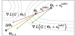
Figure 1. Update procedure of APP. The downward-pointing red line represents gradient of $\boldsymbol{L(G|\Theta)}$ and the adversarial perturbation $\boldsymbol{n_{t}^{(adv)}}$ is in the opposite direction. The green line is the gradient of loss at a perturbed position $\boldsymbol{\Theta_{t}+n_{t}^{(adv)}}$. The yellow line is the final descent direction.

3.1. APP as New Optimization Method

Eq. (3) shows that APP perturbs the parameter $\Theta$ dynamically at each iteration of gradient descent. This inspire us to look into the optimization procedure of APP. As Fig.1 illustrates, to optimize the overall loss function at step $t$, model parameter $\Theta_{t}$ will be perturbed along the perturbation direction $n_{t}^{(adv)}$. Then $\Theta_{t}$ is updated from both the gradients of $L(G|\Theta_{t})$ and the perturbed objective $L(G|\Theta_{t}+n^{(adv)}_{t})$, indicating the direction of gradient descent does not depending only on $\nabla L(G|\Theta)$. It can be viewed as an optimization strategy in essence. Therefore, we have the following theorem:

Theorem 1.

Given an unconstrained differentiable loss function $L(\Theta)$, applying APP strategy (Eq. (3)) with gradient descent is equivalent to iterative optimization based on the following strategy when updating the parameter $\Theta$:

(4) $$\begin{split}\Theta_{t+1}&=\Theta_{t}-\epsilon\Delta\Theta_{t},\\ \Delta\Theta_{t}=\nabla&L(\Theta_{t})+\lambda\nabla L(\Theta_{t}+n^{(adv)}_{t})\end{split}$$

where $\Theta_{t}$ is the value of $\Theta$ in the $t$-th iteration, $\epsilon$ is the learning rate, and $n^{(adv)}_{t}$ is the adversarial perturbation which equals $\mathop{\arg\max}_{n,||n||\leq\rho}L(\Theta_{t}+n)$.

Eq. (17) holds for every reasonable loss $L$, and it provides the way to update parameter $\Theta$ so that APP can indeed be regarded as an optimization method. Note that APP updates $\Theta$ and $n^{(adv)}$ every iteration following common used manner proposed in (Goodfellow et al., 2014).

3.2. Property of the APP Optimization Method

In order to have a deeper understanding of this optimization method, we analyze its property especially when the loss function gets stuck in the saturation region or is about to converge. We discover that the current value of perturbed loss $L(\Theta_{t}+n)$ is very close to the value of loss at last step, i.e., $L(\Theta_{t-1})$. Mathematically, we have the following theorem:

Theorem 2.

If (1) $L$ is L-smooth, i.e., $||\nabla L(\Theta_{t})-\nabla L(\Theta_{t-1})||\leqslant l||\Theta_{t}-\Theta_{t-1}||$ and (2) $||\nabla L(\Theta_{t})||\leqslant\delta$ hold where $l,\delta$ are both finite positive constants, then we have the following inequality:

(5) $$\left|\max_{||n||\leq\rho}\{L(\Theta_{t}+n)\}-L(\Theta_{t-1})\right|\leqslant(1+\lambda\epsilon l)\rho\delta+\epsilon(1+\lambda)\delta^{2}.$$

Based on Theorem. 2, when the objective gets stuck in the saturation region or is about to converge, we have the following two corollaries:

Corollary 2.1.

The perturbation in Eq. (3) can be approximated as:

(6) $$n^{(adv)}_{t}=\Theta_{t-1}-\Theta_{t}.$$

Corollary 2.2.

The AdvTNE optimization method can be formulated as:

(7) $$\begin{split}\Theta_{t+1}&=\Theta_{t}-\epsilon\Delta\Theta_{t},\\ \Delta\Theta_{t}=\nabla&L(\Theta_{t})+\lambda\nabla L(\Theta_{t-1}).\end{split}$$

Theorem. 2 and two corollaries demonstrate that the optimal adversarial perturbation $n_{t}^{(adv)}$ can be approximated as $\Theta_{t-1}-\Theta_{t}$ when the objective gets stuck in the saturation region or is about to converge, in other words, update procedure of APP can be approximated as a combination of gradient of loss at current step $t$ and the last step $t-1$. As the original method requires additional calculation of $\nabla L(\Theta_{t}+n_{t}^{(adv)})$, the training procedure will be speed up if we directly replace it with $\nabla L(\Theta_{t-1})$. Theorem. 2 provides the theoretical justification for this approximation.

We notice that Eq. (26) is similar to the formula of other well-known optimization methods, and this arouses us to investigate their relations in the next section.

3.3. Relationship with Momentum

To understand the new optimization method more intuitively, we further analyze the relationship between the APP strategy and classic optimization methods like Momentum (Ruder, 2016). We first show the update strategy of Momentum:

(8) $$\Theta_{t+1} =\Theta_{t}-\epsilon\Delta\Theta_{t},$$

(9) $$\Delta\Theta_{t}=\nabla L(\Theta_{t})+\eta\Delta\Theta_{t-1}$$

where $\eta\in(0,1)$ is a hyper-parameter controlling the weight of historical information.

In particular, Momentum computes Exponential Moving Average of the gradient sequence to run through the saturation region, which can be seen by expanding Eq. (9) as:

$$\Delta\Theta_{t} =\nabla L(\Theta_{t})+\eta\nabla L(\Theta_{t-1})+\eta^{2}\nabla L(\Theta_{t-2})+\cdots$$

(10) $$=\nabla L(\Theta_{t})+\eta\nabla L(\Theta_{t-1})+\mathcal{O}(\eta^{2})\approx\nabla L(\Theta_{t})+\eta\nabla L(\Theta_{t-1}).$$

Eq. (10) indicates that weights of gradients at previous states will decrease exponentially by $\eta$. Comparing the updating strategies of Momentum in Eq. (10) and APP in Eq. (26), it is apparent that they are similar in the parameter update procedure, especially if $\mathcal{O}(\eta^{2})$ is small enough and can be ignored. Intuitively, when the loss is about to converge or gets stuck in the saturation region, the optimal adversarial direction functions as vanishing the effect of updating; that is to say, the parameter at step $t$ is perturbed back to the last step $t-1$. Consequently, the adversarial term becomes a momentum term.

Furthermore, we conduct experiments to verify this conclusion. We compare the performance of DeepWalk optimized with Momentum and APP (i.e., AdvTNE), respectively. Experiment settings are described in Section. 5 and the results are presented on Tab. 2. We can find that utilizing APP to optimize DeepWalk achieves comparable results with Momentum-optimized DeepWalk, indicating that APP is similar to Momentum from both theory and practice. As APP performs well in network embedding, we can attribute the effectiveness to the momentum information.

We also know that APP and Momentum are similar especially when the loss function gets stuck in the saturation region or the model parameters are about to converge. As models utilizing APP like AdvTNE achieve impressive performance improvement compared with the original ones, we believe that the APP method shows its superiority over the original method in this scene. However, it raises another question: is the phenomenon of saturation region severe on network embedding? We will discuss it in the next section.

3.4. Why APP Performs Well on Network Embedding

APP, regarded as a new optimization method, decreases the loss function in a way that strengthens the momentum information, especially when the loss function is on the saturation region. However, we still have no idea why the model performance is improved when the optimization method emphasizes more on this region. In this section, we will reveal the saturation region problem on network embedding if Sigmoid is selected as the activation. Note that AdvTNE can be utilized for all Skip-gram based Network Embedding (SGNE) methods, and we take LINE as an example in the following analysis for simplicity.

Intuition

We directly post the intuitive conclusion of our theoretical analysis. In a scale-free network, the similarity $S^{+}$ of most node pairs learned by SGNE methods approaches 1, leading to indistinguishable embedding vectors of these nodes. It increases the burden on downstream tasks as it will be more challenging to distinguish these nodes or node pairs precisely. We expect to accurately learn nodes representations that can enable the downstream learner to tell slight differences between the similarity of node pairs. However, utilizing Sigmoid as the activation in SGNE models will force $S^{+}$ of node pairs with high similarity value to fall into the saturation region of the Sigmoid function. The gradients of parameters are about to vanish so that the similarity cannot be optimized anymore. Considering the APP method, an important reason it works well is that it collects the momentum information to enhance the gradient in the Sigmoid saturated region and is able to reach a better minimum.

To verify our intuition, we analyze the theoretical optimal solution of SGNE method and calculate its value in a practical situation. First, we have the following conclusion:

Theorem 3.

For sufficiently large embedding dimensionality $r$, Eq. (1) The minimum for similarity of point pair $(v_{i},v_{j})$ has the following form:

(11) $$\begin{split}S_{ij}^{+}=\frac{w_{ij}}{w_{ij}+(\frac{d_{i}d_{j}}{D})k},\end{split}$$

where $d_{i}=\sum_{j}w_{ij}$ and $D=\sum_{i}d_{i}$.

Note that it is not so difficult to meet the condition that the embedding dimensionality should be sufficiently large. As is discussed in (Levy and Goldberg, 2014b), $r\sim 100$ can also achieve satisfactory performance while satisfying $r\ll N$. The degree of nodes in a scale-free network follows a power-law distribution, meaning the degree of most nodes is very small. The number of negative sample $k$ is usually set as $3\sim 10$ in practice. $(\frac{d_{i}d_{j}}{D})k\to 0$ holds for linked node pairs $(w_{ij}>0)$, so that $S_{ij}^{+}\to 1$. It means that the similarity of linked nodes will all approximate 1. In order to have a more distinct comprehension of this result, we proved the following theorem:

Theorem 4.

Considering a scale-free network that the degree $d$ of each node follows the power-law as $d\sim P(d)\propto d^{-\alpha},\,\alpha\in(2,3)$, the number of edges is $|E|$ and the number of negative samples is $k$. Given a threshold $\gamma\in(0,1)$, the following equation holds:

(12) $$P(S^{+}_{ij}\geq\gamma)\approx\frac{(\alpha-1)^{2}}{{-\alpha+2}}\frac{\log|E|}{2|E|}\cdot(R^{\alpha-2}-1),$$

where $R=\frac{\gamma k}{2(1-\gamma)|E|}$.

The proof can be found in the Appendix. According to Eq. (34), we can calculate the expected ratio of linked nodes that their similarity $S^{+}$ is higher than a threshold $\gamma$ to the total number of edges:

(13) $$\mathbb{E}[\frac{\#(S^{+}>\gamma)}{|E|}]=\frac{|V|(|V|-1)P(S^{+}>\gamma)}{2|E|}.$$

Here is a specific example. Let $|V|=1000$, $|E|=3000$, $k=4$, $\alpha=2.5$, $\mathbb{E}[\frac{\#(S^{+}>0.9)}{|E|}]$ equals to $81.6\%$. It can be seen that the number of node pairs whose similarity falls in the Sigmoid saturation region accounts for a sufficiently large proportion. The problem of the Sigmoid saturation region is extremely severe to damage the quality of node embedding. Luckily, the APP method, which enhances its optimization power by incorporating momentum information, can achieve a remarkable result under this situation. Therefore, we believe it is one of the reasons that APP performs so well.

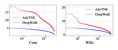
Figure 2. Comparison between DeepWalk and the corresponding AdvTNE method. The higher line represents high similarity values calculated by the node embeddings.

To verify our assumption, we make a comparison between the original DeepWalk model and AdvTNE taking DeepWalk as the base. We follow the best experiment setting and more details are elaborated in Section. 5. For simplicity, we calculate the similarity of linked nodes based on their normalized representation vectors. The simplified similarity is $\tilde{u}_{j}^{\prime}\cdot\tilde{u}_{i}$ where $\tilde{u}_{j}^{\prime}$ and $\tilde{u}_{i}$ are normalized vectors of $\vec{u}_{j}^{\prime}$ and $\vec{u}_{i}$, respectively. We select 85% node pairs that scores highest in the corresponding PPMI matrix and depict their simplified similarity. Node pairs with higher PPMI values are supposed to have higher simplified similarity scores. The results are displayed in Fig. 2 and the simplified similarity values are sorted by their PPMI values for visualization. As Figure. 2 illustrates, on the paper citation network Cora and the page-page network Wiki, the similarity values of the node pair whose embeddings are learned by AdvTNE are much higher, indicating that the APP can indeed help the base model learn higher similarities of node pairs, thus promote the model performance.

4. Another Road to Better Performance

Through the above analysis, we can conclude that (1) similarity of connected node pairs whose embeddings are learned through SGNE will concentrate on high values; (2) the Sigmoid-based loss function (i.e., loss function with Sigmoid as the activation $\sigma(\cdot)$) in SGNE has an evident saturation region effect, which increases the difficulty of convergence for the node representations. Thus, the performance in downstream tasks is substantially affected by the imperfect node representations. (3) APP solves this problem from the perspective of improving the optimization process. Intuitively, the adversarial perturbations provide the “inertial” component that contributes to a better descent and alleviates being stuck in the saturation region.

It also inspires us to find a more direct way to solve the problem of node similarities falling in the saturation region. In other words, since the Sigmoid-based loss function brings an evident saturation region effect, can we seek its substitutes for reducing this effect and improve the quality of embedding vectors? The substitute should satisfy some restrictions: (1) the activation must be bounded to guarantee the model convergence; (2) its saturation region should be small enough to enable an easier optimization to the optimal value.

Since (1) and (2) are hard to satisfy simultaneously for common-used activation, we turn to periodic functions that have considerably small saturation regions. Besides, periodic functions having many equal optimal values will reduce the optimization difficulty as the parameters can be optimized to any one of them. Motivated by this idea, we propose a new activation to Enhance the AdvTNE and we name it EATNE. The activation can be formulated as:

(14) $$\begin{split}&T_{ij}^{+}=\frac{1}{2}\left(1+\sin[\frac{\pi}{2}W_{T}(\vec{u}^{\prime}_{j}\otimes\vec{u}_{i})]\right)+\delta\\ &T_{in}^{-}=\frac{1}{2}\left(1-\sin[\frac{\pi}{2}W_{T}(\vec{u}^{\prime}_{n}\otimes\vec{u}_{i})]\right)+\delta\\ L(G|\Theta)=&-\!\!\sum_{v_{i}\in V}\!\!\sum_{v_{j}\in N_{S}(v_{i})}\!\!w_{ij}\left(\log T_{ij}^{+}\!+\!k\cdot\mathbb{E}_{v_{n}\sim P_{n}(v)}[\log T_{in}^{-}]\right).\end{split}$$

Here, we denote the node similarity between node $v_{i}$ and $v_{j}$ in EATNE as $T_{ij}^{+}$. $W_{T}\in\mathbb{R}^{1\times r}$ is a learnable parameter and $\otimes$ denotes the element-wise multiplication between the embeddings of two nodes. $\delta>0$ is a small constant to ensure that $T_{ij}^{+}$ and $T_{in}^{-}$ is greater than 0 as $\log 0\to-\infty$. Inspired by (Sitzmann et al., 2020), we apply batch normalization on the term $\vec{u}^{\prime}_{j}\otimes\vec{u}_{i}$ and $\vec{u}^{\prime}_{n}\otimes\vec{u}_{i}$ so that they follows the uniform distribution $\mathcal{U}(-1,1)$. $W_{T}$ is also initilized as $W_{T}\sim\mathcal{U}(-\sqrt{6/r},\sqrt{6/r})$ to ensure that $W_{T}(\vec{u}^{\prime}_{j}\otimes\vec{u}_{i})\sim\mathcal{N}(0,1)$ and $W_{T}(\vec{u}^{\prime}_{n}\otimes\vec{u}_{i})\sim\mathcal{N}(0,1)$. Here $\mathcal{N}(\cdot,\cdot)$ is the normal distribution. Eq. (14) can be viewed as a Sine-based loss function.

It is not hard to verify that this activation satisfies the first restriction. To examine the second restriction with this activation and to show the superiority of the Sine-based loss function, we compare the learning progress with the Sigmoid-based one. With Sigmoid-based loss function, the optimal value can be reached by

(15) $$\begin{split}&S^{+}_{ij}=\frac{1}{1+\exp(-\vec{u}^{\prime}_{j}\cdot\vec{u}_{i})}=1\Rightarrow\vec{u}^{\prime}_{j}\cdot\vec{u}_{i}\to\infty.\end{split}$$

For Sine-based loss function, the optimal value is

(16) $$\begin{split}\frac{1}{2}&\left(1+\sin[\frac{\pi}{2}W_{T}(\vec{u}^{\prime}_{j}\otimes\vec{u}_{i})]\right)+\delta=1\Rightarrow\\ &W_{T}(\vec{u}^{\prime}_{j}\otimes\vec{u}_{i})=\frac{2}{\pi}\arcsin(1-2\delta).\end{split}$$

In practice, $\vec{u}^{\prime}_{j}\cdot\vec{u}_{i}$ is hard to reach $\infty$ for computer precision. In addition, when $\vec{u}^{\prime}_{j}\cdot\vec{u}_{i}\to\infty$, the norm of $\Delta\Theta$ meets the expression that $||\Delta\Theta||\sim S^{+}_{ij}(1-S^{+}_{ij})\approx 0$, indicating that the parameters almost cannot be updated after certain iteration. However, the range of arcSine function is finite, enabling the fast convergence of the node representation vectors. Besides, when $T^{+}_{ij}\to 1$, it holds that $||\Delta\Theta||\sim\sqrt{\delta(1-\delta)}$, indicating the norm of $\Delta\Theta$ is much bigger than that of Sigmoid-based loss function. In conclusion, our Sine-base loss function satisfies the two necessary restrictions and it is supposed to be effective on network embedding.

Table 1. Statistics of benchmark datasets

Datasets	# Nodes	# Edges	# Avg.Degree	# Labels
Cora	2708	5278	1.95	7
Citeseer	3264	4551	1.39	6
Wiki	2363	11596	4.91	17
PubMed	19717	88648	4.50	3

5. Experiment

We conduct experiments on real-world networks on node classification and link prediction task to verify our analysis:

• Q1: Can APP achieve results comparable to Momentum optimization if APP and Momentum are similar in the formula?

• Q2: How does our new activation perform compared to the state-of-the-art network embedding models?

5.1. Experiment Setup

5.1.1. Datasets

We conduct experiments on four real-world datasets. Cora, Citeseer, and PubMed (Yang et al., 2016) are all paper citation networks where nodes correspond to paper and edges represent citation links. Wiki (Sen et al., 2008) is a network with many web pages as its nodes and hyperlinks between web pages as its edges. We delete nodes with self-loops and zero degrees on original datasets. Statistics of these datasets are summarized in Tab. 1.

Table 2. Comparison of AS and NM on Cora, Wiki and Citeseer, revealing the similarity of APP and Momentum in practice.

Ratio	Mean	1%	2%	3%	4%	5%	6%	7%	8%	9%	10%	20%	30%	40%	50%	60%	70%	80%	90%
Cora_AS	74.48	55.06	62.64	65.38	67.83	69.54	69.51	71.22	71.99	73.24	74.78	78.21	80.27	81.84	82.77	83.38	83.51	84.06	85.42
Cora_NM	76.32	63.32	67.81	69.20	71.15	73.37	73.55	74.51	75.36	75.54	76.35	79.88	80.79	81.47	81.74	82.05	81.91	82.32	83.51
Wiki_AS	56.71	34.19	44.69	48.18	51.02	51.77	51.96	54.37	54.62	55.77	56.36	60.21	62.71	63.65	64.80	65.64	66.04	67.34	67.43
Wiki_NM	56.87	36.25	46.56	49.59	52.25	52.57	54.70	55.39	55.05	56.68	57.01	59.76	62.35	62.93	63.42	64.22	64.37	64.93	65.57
Citeseer_AS	51.47	36.45	40.45	42.76	43.78	46.28	47.31	48.00	48.54	50.55	50.97	55.11	56.86	58.29	58.71	59.55	60.83	60.32	61.68
Citeseer_NM	51.56	36.28	40.43	43.38	44.46	46.88	47.36	48.74	49.02	50.71	50.79	55.07	57.47	58.41	58.93	59.82	60.59	59.98	59.69

Table 3. Accuracy(%) of multi-class classification on Cora

Ratio	Mean	1%	2%	3%	4%	5%	6%	7%	8%	9%	10%	20%	30%	40%	50%	60%	70%	80%	90%
DeepWalk	74.55	59.57	63.54	66.75	69.43	70.54	70.82	71.77	72.66	73.60	74.43	77.75	79.30	80.50	80.89	82.31	82.12	82.32	83.58
LINE	66.02	50.93	56.16	60.55	62.14	63.89	63.46	65.09	65.07	66.18	66.53	68.73	70.15	70.31	71.07	70.93	72.20	72.16	72.80
node2vec	74.71	59.18	64.03	66.94	69.20	70.57	71.00	71.45	72.60	73.33	74.16	77.57	79.93	80.84	81.82	82.14	82.85	83.03	84.13
GF	41.35	20.79	29.76	33.65	34.68	36.13	37.65	39.01	38.93	40.28	40.53	44.85	46.80	48.45	49.75	49.63	50.23	51.75	51.40
GraRep	71.45	55.01	60.85	66.12	68.09	67.26	70.77	70.81	71.27	71.47	72.73	74.42	75.68	75.70	76.13	78.13	77.28	77.43	76.97
GraphSage	53.62	31.51	38.79	44.29	45.07	47.29	49.77	50.43	51.77	53.92	54.18	58.24	59.59	62.07	62.89	63.55	63.79	62.88	65.09
AdvTNE	75.14	58.95	65.18	67.21	68.62	71.19	71.45	72.41	73.39	73.81	75.15	77.88	79.94	81.03	82.22	82.97	83.11	83.71	84.24
Cleora	70.99	54.29	60.97	62.62	65.68	68.51	68.65	68.82	71.17	71.04	72.08	73.85	75.62	76.57	76.82	76.98	77.48	77.90	78.75
EATNE	76.93	60.30	66.28	70.56	72.43	74.96	74.60	75.44	76.64	77.33	77.55	80.12	81.09	81.57	82.47	82.90	83.06	83.47	84.02

Table 4. Accuracy(%) of multi-class classification on Citeseer

Ratio	Mean	1%	2%	3%	4%	5%	6%	7%	8%	9%	10%	20%	30%	40%	50%	60%	70%	80%	90%
Deepwalk	51.76	38.53	41.53	43.63	44.41	46.62	47.25	48.35	48.63	49.59	50.65	55.06	57.46	58.15	59.15	59.43	61.21	60.46	61.50
LINE	41.94	35.19	36.55	39.06	38.49	40.34	40.95	41.33	40.79	41.80	41.87	42.99	43.77	44.40	45.20	44.98	45.19	45.91	46.09
node2vec	52.08	39.62	42.19	44.54	45.62	46.92	48.17	48.63	49.36	50.27	50.91	55.08	57.53	58.55	59.29	59.77	60.54	60.28	60.21
GF	30.21	21.00	23.22	24.54	25.96	26.20	27.61	28.07	28.01	28.22	29.12	31.81	33.80	34.92	35.00	35.54	35.67	37.55	37.61
GraRep	48.17	35.37	40.10	41.78	44.79	45.59	46.20	47.93	47.38	47.72	47.87	50.39	51.88	52.05	53.20	53.00	54.00	54.80	53.08
GraphSage	30.97	20.94	23.54	24.04	25.93	26.41	26.96	28.62	28.29	29.58	30.52	32.97	35.40	35.60	37.43	36.88	37.84	37.43	39.02
AdvTNE	53.14	39.02	41.94	44.77	45.21	47.43	49.06	49.72	51.09	51.61	52.72	57.06	59.56	60.14	60.64	61.30	61.87	61.23	62.14
Cleora	52.85	42.14	44.10	48.19	48.67	50.39	51.24	51.32	52.61	52.60	52.93	54.71	55.97	56.17	57.04	57.50	58.67	58.18	58.93
EATNE	54.87	38.10	44.37	47.15	48.62	50.98	51.95	53.22	53.44	54.55	54.82	58.05	59.91	60.63	60.96	61.85	62.66	62.89	63.46

Table 5. Accuracy(%) of multi-class classification on Wiki

Ratio	Mean	1%	2%	3%	4%	5%	6%	7%	8%	9%	10%	20%	30%	40%	50%	60%	70%	80%	90%
DeepWalk	57.81	34.14	46.01	49.35	52.02	52.34	54.51	55.41	56.30	57.67	58.69	61.85	63.49	64.65	65.52	66.06	66.29	67.67	68.69
LINE	48.59	30.67	39.73	42.58	45.05	46.00	46.89	48.18	47.64	48.81	49.09	51.71	52.88	53.03	53.61	53.82	54.40	54.44	56.16
node2vec	57.47	35.40	45.76	49.20	51.13	51.10	53.87	55.46	55.55	57.14	57.58	60.71	63.54	64.35	65.25	65.97	66.21	67.55	68.69
GF	41.84	20.37	26.45	30.48	34.22	37.21	37.69	38.09	40.82	41.25	41.71	46.42	48.65	49.97	50.80	51.67	53.03	52.01	52.28
GraRep	57.79	32.57	44.08	49.00	53.62	55.26	55.65	56.01	57.90	58.11	59.00	62.17	64.20	64.64	65.00	65.41	65.77	65.64	66.16
GraphSage	46.91	25.38	33.20	36.36	39.86	40.47	43.26	45.15	45.59	46.51	47.10	51.04	53.61	54.38	54.48	56.21	56.73	57.32	57.72
AdvTNE	57.83	35.56	45.89	49.35	52.15	51.67	53.75	54.77	55.66	56.52	56.85	61.29	63.57	65.50	66.12	66.72	67.31	69.15	69.07
Cleora	56.66	33.11	44.08	49.42	50.59	51.65	53.77	56.09	55.52	57.02	57.78	60.10	62.12	63.19	63.59	63.66	65.42	66.49	66.24
EATNE	59.14	34.69	47.13	50.93	53.80	53.41	56.08	57.83	57.29	58.81	59.37	62.36	64.99	65.98	66.94	67.29	67.86	68.56	71.18

5.1.2. Baseline Methods

We compare EATNE with the following baseline models:

• Graph Factorization (GF) (Ahmed et al., 2013): GF utilizes a stochastic gradient descent technique to factorizes the adjacency matrix, and it can scale to large networks.

• DeepWalk (Perozzi et al., 2014): DeepWalk obtains node embedding by applying the skip-gram model on node sequences sampled from the truncated random walk.

• LINE (Tang et al., 2015): LINE takes into consideration node co-occurrence probability and node conditional probability to preserve network structural proximities. The problem of expensive computation is also alleviated through the negative sampling approach.

• node2vec (Grover and Leskovec, 2016): node2vec samples node sequences with a more flexible method and balances the local and global structural properties.

• GraRep (Cao et al., 2015): GraRep learns node embeddings by using the SVD technique to different k-step probability transition matrix and concatenating all k-step representations.

• GraphSage (Hamilton et al., 2017): GraphSage collects neighborhood information by constructing a local computing graph and inductively learns node embeddings.

• AdvTNE (Dai et al., 2019): AdvT adopts adversarial training methods on network embedding by adding perturbation to embedding, which can be treated as a regularization term.

• Cleora (Rychalska et al., 2021): Cleora is a efficient unsupervised network embedding method that does not optimize an explicit objective and sample positive or negative examples.

5.1.3. Experiment Settings

We apply AdvTNE and EATNE on DeepWalk and the walk length, walks per node, window size, negative size, regularization strength and batch size are set to 40, 1, 5, 5, 1 and 2048, respectively. The dimension of embedding vectors is 128 and we training each model for 100 epochs. We utilize the recommended hyper-parameters and optimization methods of baseline models mentioned in the corresponding paper. Random search (Bergstra and Bengio, 2012) is applied to find the optimal adversarial noise level $\epsilon$, regularization factor $\lambda$ and learning rate. The search range for $\epsilon$ is 0.1$\sim$5. We set 1e-5$\sim$1 as the search range for learning rate and 1e-2$\sim$1e3 for the regularization factor $\lambda$.

5.1.4. Downstream Task

We select link prediction and node classification as the downstream tasks to evaluate the quality of representation vectors. The experiment results are averaged over ten runs on both tasks. In link prediction, $80\%$ of the edges are randomly sampled as the positive training samples with the same amount of negative training samples, i.e., node pair without direct edge. The rest $20\%$ edges together with two times of negative samples are sampled to construct the test set. AUC is adopted to measure the performance of link prediction as we train an $L_{2}$-SVM classifier to predict links with the edge features like other works (Dai et al., 2019). Here we use the Hadamard product of representation vectors from the endpoints of the same edge as the edge features. As for node classification, 18 training ratios, ranging from $1\%\sim 9\%$ and $10\%\sim 90\%$, are set to train the support vector classifier. It is designed to demonstrate the ability under different proportions of training data so we utilize accuracy as the metric.

5.2. Similarity of APP and Momentum (Q1)

To support our claim that AdvTNE is a Momentum-like optimization method, we compare two models on the node classification task: AdvtNE optimized with SGD (AS) and Non-AdvTNE optimized with Momentum (NM, i.e., DeepWalk only). The experiments are conducted on Cora, Wiki and Citeseer. The adversarial noise level $\epsilon$ is 0.9 for Cora, 1.1 for Citeseer and 0.6 for Wiki, respectively. We set 0.001 as learning rate and 1.0 as the regularization factor $\lambda$ for AS following the original paper. For NM, learning rate is 0.1040 for Wiki, 0.0276 for Citeseer and 0.4524 for Cora. As shown in Table. 2, NM can achieve comparable results compared with AS. When AdvTNE is optimized by SGD, based on Theorem. 1, it can be viewed as using APP to optimize DeepWalk, revealing that APP is indeed similar to Momentum from these results. Note that original AdvTNE is optimized with Adam and its performance is slightly higher. We can also discover that NM surpasses AS in the low training ratio case, demonstrating the strong generalization ability of Momentum in the semi-supervised learning scenario.

5.3. Remarkable results of EATNE (Q2)

5.3.1. Node Classification

In this section, we conduct a multi-class classification on three graph datasets with different training ratios to simulate the semi-supervised scene. The results are organized and presented on Table. 3 - 5. It can be observed that EATNE achieves impressive performance, especially the best average classification accuracy on 18 training ratios for all three graph datasets. The relative average error rate of node classification is reduced by 7.2% on Cora, 3.7% on Citeseer and 3.1% on Wiki. Moreover, we obtain the best results on 45/54 trials, demonstrating the benefit of Sine-based loss function in semi-supervised scenarios. Note that although Cora and Citeseer are similar in network scale and number of classes, the imbalanced class distribution contributes to the difference of classification accuracy between Cora and Citeseer. By the way, to simulate the scene that the graphs only contain structure information, we generate random features as inputs for GraphSage, or it will be unfair to other methods if we use original node features.

5.3.2. Link Prediction

Link prediction plays an essential role in real-world applications for the capacity of mining underlying relations between entities. We carry out link prediction on four graph datasets to demonstrate the effectiveness of our methods against other state-of-the-art methods. The results are summarized on Table. 6. As we can see that EATNE achieves competitive results on all four datasets compared with other methods. Specifically, based on AdvTNE, the AUC score increases by $2.63\%$ on Cora, $6.67\%$ on Citeseer, $8.22\%$ on Wiki and $8.46\%$ on PubMed, which shows that the Sine-based loss function can further promote performance of models applying APP. Besides, EATNE also performs well on the largest network datasets PubMed, revealing its great potential in scaling to large-scale graphs.

6. Related Work

Network Embedding can be categorized into inductive learning methods (Hamilton et al., 2017) and transductive learning methods (Tang et al., 2015; Cao et al., 2015; Grover and Leskovec, 2016). Inductive learning optimizes parameters of a well-designed neural network, following a node attributes-based message passing mechanism. Directly optimizing the node embeddings, transductive learning performs pretty well on the scene of unsupervised learning without node attributes and becomes the focus of this paper. Inspired by word embedding methods, some methods based on the skip-gram model word2vec are proposed (Perozzi et al., 2014; Tang et al., 2015; Grover and Leskovec, 2016). Besides, (Levy and Goldberg, 2014b) proved the equivalence between skip-gram models with negative-sampling and matrix factorization, which led to new proximity metrics under the matrix factorization proximity framework (Yang et al., 2015; Cao et al., 2015).

Table 6. AUC score for link prediction

Dataset	Cora	Citeseer	Wiki	PubMed
DeepWalk	0.628$\pm$0.014	0.528$\pm$0.010	0.525$\pm$0.007	0.503$\pm$0.001
LINE	0.606$\pm$0.015	0.514$\pm$0.009	0.506$\pm$0.004	0.502$\pm$0.002
node2vec	0.626$\pm$0.011	0.522$\pm$0.010	0.526$\pm$0.004	0.506$\pm$0.003
GF	0.500$\pm$0.003	0.505$\pm$0.011	0.507$\pm$0.003	0.502$\pm$0.004
GraRep	0.501$\pm$0.002	0.502$\pm$0.009	0.506$\pm$0.005	0.503$\pm$0.003
GraphSage	0.504$\pm$0.002	0.500$\pm$0.006	0.501$\pm$0.005	0.500$\pm$0.002
AdvTNE	0.647$\pm$0.008	0.520$\pm$0.010	0.532$\pm$0.004	0.523$\pm$0.006
Cleora	0.641$\pm$0.025	0.526$\pm 0.022$	0.524$\pm$0.026	0.512$\pm$0.004
EATNE	0.665$\pm$0.004	0.544$\pm$0.008	0.566$\pm$0.005	0.551$\pm$0.002

Adversarial Training is introduced in Computer Vision, Speech Recognition and Natural Language Processing for promotion of model robustness (Miyato et al., 2015; Madry et al., 2017; Shafahi et al., 2019; Sun et al., 2018; Liu et al., 2019; Drexler and Glass, 2018; Miyato et al., 2018; Zhu et al., 2019; Liu et al., 2020). (Miyato et al., 2015) proposes virtual adversarial training on the basis of optimization of KL-divergence based robustness against local perturbations. Adversarial training also achieves impressive performance on supervised and semi-supervised learning scenes (Miyato et al., 2018) for the design of unlabelled adversarial direction. (Shaham et al., 2018) explains its mechanism by the perspective of robust optimization. Researchers introduce Adversarial Training into network embedding for its great success. Some works apply perturbations to network structures (Dai et al., 2018; Xu et al., 2019), others on the node or edge attributes (Wang et al., 2019c; Jin and Zhang, 2019). It is worth mentioning that Adversarial training based network embedding methods are different from Generative Adversarial Network (GAN) based ones (Wang et al., 2018; Hong et al., 2019; Gao et al., 2019). GAN based network embedding methods utilize a mini-max game between connectivity generators and corresponding discriminators to obtain representations.

Although some researches introduce Adversarial Training to generate adversarial perturbations on networks in various ways, few of them pay attention to perturbations in parameter space. AdvTNE (Dai et al., 2019) integrates adversarial training with network embedding in a different manner that perturbations are added not in input space but parameter space. Inspired by this idea, in computer vision, some researches introduce adversarial perturbations on parameters (APP) for better generalization ability. (Foret et al., 2020) adopts APP to seek for parameters where the training loss of the entire neighborhoods are very low; (Wu et al., 2020) utilizes APP from the perspective of flattening the weight loss landscape; (Zheng et al., 2020) regards APP as a regularization to reach a flatter minima of a maximized empirical loss. To summarize, APP in AdvTNE has broadened the way of designing adversarial training so that it is well worth investigating the mechanism behind it, which is the main idea of this paper.

7. Conclusion

In this paper, we study APP theoretically from an optimization perspective, explore the reason for its impressive effectiveness, and propose a new activation based on AdvTNE. We first prove that APP can be interpreted as an optimization method and analyze its relationship with Momentum. One reason for its outstanding performance is that it provides momentum information to accelerate optimization on the saturation region. Detailed experiments verify the similarity between APP and Momentum on node classification tasks. To address the saturation region problem caused by Sigmoid activation, we design a new activation to obtain high-quality representations more easily. Our method achieves satisfactory results on four data sets on both node classification and link prediction tasks, which practically demonstrates the superiority of our activation. Furthermore, the Sine-based activation is expected to address limitations brought by Sigmoid-based activation in similar scenarios. Especially, it is reasonable to promote it to word embedding methods as they have similar paradigms and they both obey the power-law distribution. We will apply APP as a new optimization method and the Sine-based activation to tackle the Sigmoid saturation region problem in the aforementioned fields in future work.

8. Appendix

8.1. Proof of Theorem 1

Theorem 1.

Given an unconstrained differentiable loss function $L(\Theta)$, applying APP strategy with gradient descent is equivalent to iterative optimization based on the following strategy when updating the parameter $\Theta$:

(17) $$\begin{split}\Theta_{t+1}&=\Theta_{t}-\epsilon\Delta\Theta_{t},\\ \Delta\Theta_{t}=\nabla&L(\Theta_{t})+\lambda\nabla L(\Theta_{t}+n^{(adv)}_{t})\end{split}$$

where $\Theta_{t}$ is the value of $\Theta$ in the $t$-th iteration, $\epsilon$ is the learning rate, and $n^{(adv)}_{t}$ is the adversarial perturbation which equals $\mathop{\arg\max}_{n,||n||\leq\rho}L(\Theta_{t}+n)$.

Proof.

Given the parameter at current step $t$ as $\Theta_{t}$, firstly we expect to maximize $L(\Theta_{t}+n)$ in the adversarial perturbation generation step:

(18) $$n^{(adv)}_{t}=\mathop{\arg\max}_{n,||n||\leq\rho}L(\Theta_{t}+n).$$

As soon as $n^{(adv)}_{t}$ is determined, the objective is a function only related to $\Theta_{t}$ as $L(\Theta_{t})+\lambda L(\Theta_{t}+n^{(adv)}_{t})$

We optimize this objective through gradient descent with learning rate $\epsilon$:

(19) $$\begin{split}\Theta_{t+1}&=\Theta^{t}-\epsilon\Delta\Theta_{t},\\ \Delta\Theta_{t}=\nabla&L(\Theta_{t})+\lambda\nabla L(\Theta_{t}+n^{(adv)}_{t}).\end{split}$$

This updating procedure can be considered from another aspect: considering the objective function $L(\Theta_{t})$, when updating $\Theta_{t}$, an additional term $\lambda\nabla L(\Theta_{t}+n^{(adv)}_{t})$ is also utilized besides the gradient $\nabla L(\Theta_{t})$. As a result, it is reasonable to regard it as an optimization method. Thus, the theorem is proved. ∎

8.2. Proof of Theorem 2

Theorem 2.

If (1) $L$ is L-smooth, i.e., $||\nabla L(\Theta_{t})-\nabla L(\Theta_{t-1})||\leqslant l||\Theta_{t}-\Theta_{t-1}||$ and (2) $\exists t,s.t.||\nabla L(\Theta_{t})||\leqslant\delta$ hold where $l,\delta$ are both finite positive constants, then the following inequality holds:

(20) $$\left|\max_{||n||\leq\rho}\{L(\Theta_{t}+n)\}-L(\Theta_{t-1})\right|\leqslant(1+\lambda\epsilon l)\rho\delta+\epsilon(1+\lambda)\delta^{2}.$$

Proof.

First, $L(\Theta_{t})$ can be written as:

(21) $$L\left(\Theta_{t}\right) =L\left(\Theta_{t-1}\right)+\nabla L\left(\Theta_{t-1}\right)^{\top}\left(\Theta_{t}-\Theta_{t-1}\right)+\mathcal{O}\left(\left\|\Theta_{t}-\Theta_{t-1}\right\|^{2}\right)$$

$$\approx L\left(\Theta_{t-1}\right)+\nabla L\left(\Theta_{t-1}\right)^{\top}\left(\Theta_{t}-\Theta_{t-1}\right)$$

$$=L\left(\Theta_{t-1}\right)-\epsilon\nabla L(\Theta_{t-1})^{\top}\left[\nabla L\left(\Theta_{t-1}\right)+\lambda\nabla L\left(\Theta_{t-1}+n_{t-1}\right)\right]$$

$$=L\left(\Theta_{t-1}\right)-\epsilon\nabla L(\Theta_{t-1})^{\top}\nabla L\left(\Theta_{t-1}\right)$$

$$-\lambda\epsilon\nabla L(\Theta_{t-1})^{\top}\nabla L\left(\Theta_{t-1}+n_{t-1}\right).$$

We denote the last term $\nabla L(\Theta_{t-1})^{\top}\nabla L\left(\Theta_{t-1}+n_{t-1}\right)$ as $*$ and approximate it as:

(22) $$* =\nabla L(\Theta_{t-1})^{\top}\left[\nabla L\left(\Theta_{t-1}\right)+\nabla L\left(\Theta_{t-1}+n\right)-\nabla L\left(\Theta_{t-1}\right)\right]$$

$$\leqslant\left\|\nabla L\left(\Theta_{t-1}\right)\right\|^{2}+\left\|\nabla L\left(\Theta_{t-1}\right)\right\|\cdot\left\|\nabla L\left(\Theta_{t-1}+n\right)-\nabla L\left(\Theta_{t-1}\right)\right\|$$

$$\leqslant\delta^{2}+\delta l\|\Theta_{t-1}+n-\Theta_{t-1}\|$$

$$\leqslant\delta^{2}+\rho\delta l.$$

Secondly, we approximate $\max_{||n||\leq\rho}\{L(\Theta_{t}+n)\}$ via a first-order Taylor expansion as:

(23) $$\max_{||n||\leq\rho}\{L(\Theta_{t}+n)\}$$

$$\approx L\left(\Theta_{t}\right)+\max_{||n||\leq\rho}\nabla L\left(\Theta_{t}\right)^{\top}\cdot n$$

$$\approx L\left(\Theta_{t}\right)+\rho\left\|\nabla L\left(\Theta_{t}\right)\right\|.$$

The maximum is obtained when $n=\rho\nabla L\left(\Theta_{t}\right)/\left\|\nabla L\left(\Theta_{t}\right)\right\|$. Thus, by combining Eq. (21) - (23) we have:

(24) $$\left|\max_{||n||\leq\rho}\{L(\Theta_{t}+n)\}-L(\Theta_{t-1})\right|$$

$$\approx \left|L\left(\Theta_{t}\right)+\rho\left\|\nabla L\left(\Theta_{t}\right)\right\|-L(\Theta_{t-1})\right|$$

$$\leqslant \left|L\left(\Theta_{t}\right)+\rho\left\|\nabla L\left(\Theta_{t}\right)\right\|-\{L\left(\Theta_{t}\right)+\epsilon\nabla L(\Theta_{t-1})^{\top}\nabla L\left(\Theta_{t-1}\right)+\lambda\epsilon*\}\right|$$

$$= \left|\rho\left\|\nabla L\left(\Theta_{t}\right)\right\|-\epsilon\left\|\nabla L(\Theta_{t-1})\right\|^{2}-\lambda\epsilon*\right|$$

$$\leqslant \rho\delta+\epsilon\delta^{2}+\lambda\epsilon\delta^{2}+\lambda\epsilon\rho\delta l$$

$$= (1+\lambda\epsilon l)\rho\delta+\epsilon(1+\lambda)\delta^{2}.$$

The theorem is proved. ∎

Based on Theorem. 2, when the objective is stuck in the saturation region or is about to converge, we have the following two corollaries:

Corollary 2.1.

The perturbation in Eq. (3) can be approximated as:

(25) $$n^{(adv)}_{t}=\Theta_{t-1}-\Theta_{t}.$$

Corollary 2.2.

The AdvTNE optimization methods can be formulated as:

(26) $$\begin{split}\Theta_{t+1}&=\Theta_{t}-\epsilon\Delta\Theta_{t},\\ \Delta\Theta_{t}=\nabla&L(\Theta_{t})+\lambda\nabla L(\Theta_{t-1}).\end{split}$$

Proof.

When the objective is optimized to the saturation region or is about to converge, the bound of gradient norm $\delta$ is quite small. Thus, $\left|\max_{||n||\leq\rho}\{L(\Theta_{t}+n)\}-L(\Theta_{t-1})\right|\approx 0$. We have $\max_{||n||\leq\rho}\{L(\Theta_{t}+n)\}\approx L(\Theta_{t-1})$. $\Theta_{t}+n\approx\Theta_{t-1}$ is the sufficient condition for $\max_{||n||\leq\rho}\{L(\Theta_{t}+n)\}\approx L(\Theta_{t-1})$. Given that we only need to find a suitable solution of $n$, so that we have:

(27) $$n^{(adv)}_{t}=\Theta_{t-1}-\Theta_{t}.$$

Replacing the $n^{(adv)}_{t}$ in Theorem. 17, we can easily obtain:

(28) $$\begin{split}\Theta_{t+1}&=\Theta_{t}-\epsilon\Delta\Theta_{t},\\ \Delta\Theta_{t}=\nabla&L(\Theta_{t})+\lambda\nabla L(\Theta_{t-1}).\end{split}$$

These two corollaries have been proven. ∎

8.3. Proof of Theorem 3

Theorem 3.

For sufficiently large embedding dimensionality $r$, the minimum for similarity of point pair $(v_{i},v_{j})$ for SGNE objective has the following form:

(29) $$\begin{split}S_{ij}^{+}=\frac{w_{ij}}{w_{ij}+(\frac{d_{i}d_{j}}{D})k},\end{split}$$

where $d_{i}=\sum_{j}w_{ij}$ and $D=\sum_{i}d_{i}$

Proof.

Simplify the objective of SGNE as:

(30) $$\begin{split}L&=\sum_{v_{i}\in V}\sum_{v_{j}\in N_{S}(v_{i})}w_{ij}\left(\log S_{ij}^{+}+k\cdot\mathbb{E}_{v_{n}\sim P_{n}(v)}[\log S_{in}^{-}]\right)\\ &=\sum_{v_{i}\in V}\sum_{v_{j}\in N_{S}(v_{i})}w_{ij}\log S_{ij}^{+}+k\sum_{v_{i}\in V}d_{i}\cdot\mathbb{E}_{v_{n}\sim P_{n}(v)}[\log S_{in}^{-}]\\ &=\sum_{v_{i}\in V}\sum_{v_{j}\in V}w_{ij}\log S_{ij}^{+}+\frac{kd_{j}d_{i}}{D}\log(1-S_{ij}^{+}).\end{split}$$

Since embedding dimensionality $r$ is sufficiently large, each $S_{ij}^{+}$ can assume a value independently of the others (Levy and Goldberg, 2014b). We consider the local objective for $S_{ij}^{+}$:

(31) $$L_{ij}=w_{ij}\log S_{ij}^{+}+\frac{kd_{j}d_{i}}{D}\log(1-S_{ij}^{+}).$$

Let the gradient $\nabla L_{ij}(S_{ij}^{+})$ be equal to 0:

(32) $$\nabla L_{ij}(S_{ij}^{+})=\frac{w_{ij}}{S_{ij}^{+}}+\frac{kd_{j}d_{i}}{D(1-S_{ij}^{+})}=0.$$

We have

(33) $$S_{ij}^{+}=\frac{w_{ij}}{w_{ij}+(\frac{d_{i}d_{j}}{D})k}.$$

Thus, the theorem has been proved. ∎

8.4. Proof of Theorem 4

Theorem 4.

Considering a scale-free network that the degree $d$ of each node follows the power-law as $d\sim P(d)\propto d^{-\alpha},\,\alpha\in(2,3)$, the number of edges is $|E|$ and the number of negative samples is $k$. Given a threshold $\gamma\in(0,1)$, the following equation holds:

(34) $$P(S^{+}_{ij}\geq\gamma)\approx\frac{(\alpha-1)^{2}}{{-\alpha+2}}\frac{\log|E|}{2|E|}\cdot(R^{\alpha-2}-1),$$

where $R=\frac{\gamma k}{2(1-\gamma)|E|}$.

Proof.

For brevity, let $t_{ij}=\frac{w_{ij}}{d_{i}d_{j}}$ and $D=2|E|$, and the probability can be represented as follows:

(35) $$P(S^{+}_{ij}\geq\gamma)=P(\frac{w_{ij}}{d_{i}d_{j}}\geq\frac{\gamma}{1-\gamma}\frac{k}{D})=P(t_{ij}\geq R).$$

Following the definition of cumulative probability and the law of total probability, we have:

(36) $$\begin{split}P(t_{ij}\geq R)&=\sum_{t_{ij}=R}^{\infty}p(t_{ij})=\sum_{t_{ij}=R}^{\infty}\sum_{c_{ij}=1}^{\infty}p(t_{ij}|c_{ij})p(c_{ij}),\end{split}$$

where $c_{ij}=d_{i}d_{j}$. Since we use LINE objective, $w_{ij}\in\{0,1\}$. Remind that $t_{ij}=0$ if $w_{ij}=0$, therefore, we only need to calculate the probability when $w_{ij}=1$ i.e. $t_{ij}=\frac{1}{c_{ij}}\geq R$, which leads to $c_{ij}\leq\frac{1}{R}$. Eq. (36) can be rewritten as:

(37) $$\begin{split}P(t_{ij}\geq R)=\sum_{c_{ij}=1}^{\frac{1}{R}}\sum_{t_{ij}=R}^{\infty}p(t_{ij}|c_{ij})p(c_{ij})\end{split}$$

Consider the summation: $\sum_{t_{ij}=R}^{\infty}p(t_{ij}|c_{ij},D)$, following the configuration model (Kryven, 2017), given $d_{i},d_{j}$ and $D$, it can be reduced as $\frac{c_{ij}}{D}$.

(38) $$\begin{split}P(t_{ij}\geq R)&=\sum_{c_{ij}=1}^{\frac{1}{R}}\frac{c_{ij}}{D}p(c_{ij}).\\ \end{split}$$

Remember that the degree follows Power-law distribution of which Probability Density Function is $f_{d}(d)=(\alpha-1)d^{-\alpha}$ (Clauset et al., 2009), we have

(39) $$\begin{split}P(t_{ij}\geq R)&\approx\int_{1}^{\frac{1}{R}}\frac{c_{ij}}{D}f_{c}(c_{ij})\,dc_{ij}\\ &=\frac{1}{D}\int_{1}^{\frac{1}{R}}c_{ij}\,dc_{ij}\int_{1}^{|E|}\frac{f_{d}(\frac{c_{ij}}{d_{j}})f_{d}(d_{j})}{d_{j}}\,dd_{j}\\ &=\frac{1}{D}\int_{1}^{\frac{1}{R}}c_{ij}\,dc_{ij}\int_{1}^{|E|}\frac{(\alpha-1)^{2}c_{ij}^{-\alpha}}{d_{j}}\,dd_{j}\\ &=\frac{(\alpha-1)^{2}}{D}\int_{1}^{\frac{1}{R}}c_{ij}^{-\alpha+1}\log|E|\,dc_{ij}\\ &=\frac{(\alpha-1)^{2}}{{-\alpha+2}}\frac{\log|E|}{2|E|}\cdot(R^{\alpha-2}-1)\end{split}$$

Thus, the theorem has been proved. ∎

References

- (1)
- Ahmed et al. (2013) Amr Ahmed, Nino Shervashidze, Shravan Narayanamurthy, Vanja Josifovski, and Alexander J Smola. 2013. Distributed large-scale natural graph factorization. In Proceedings of the 22nd international conference on World Wide Web. 37–48.
- Bergstra and Bengio (2012) James Bergstra and Yoshua Bengio. 2012. Random search for hyper-parameter optimization. The Journal of Machine Learning Research (2012).
- Cao et al. (2015) Shaosheng Cao, Wei Lu, and Qiongkai Xu. 2015. GraRep: Learning Graph Representations with Global Structural Information. In ACM International Conference on Information and Knowledge Management. 891–900.
- Chen et al. (2021) Xu Chen, Lun Du, Mengyuan Chen, Yun Wang, Qingqing Long, and Kunqing Xie. 2021. Fast Hierarchy Preserving Graph Embedding via Subspace Constraints. In IEEE International Conference on Acoustics, Speech and Signal Processing.
- Clauset et al. (2009) Aaron Clauset, Cosma Rohilla Shalizi, and Mark EJ Newman. 2009. Power-law distributions in empirical data. SIAM review 51, 4 (2009), 661–703.
- Cook and Holder (2006) Diane J Cook and Lawrence B Holder. 2006. Mining graph data. John Wiley & Sons.
- Dai et al. (2018) Hanjun Dai, Hui Li, Tian Tian, Xin Huang, Lin Wang, Jun Zhu, and Le Song. 2018. Adversarial attack on graph structured data. arXiv preprint arXiv:1806.02371 (2018).
- Dai et al. (2019) Quanyu Dai, Xiao Shen, Liang Zhang, Qiang Li, and Dan Wang. 2019. Adversarial Training Methods for Network Embedding. In The World Wide Web Conference. ACM, 329–339.
- Deng et al. (2019) Zhijie Deng, Yinpeng Dong, and Jun Zhu. 2019. Batch virtual adversarial training for graph convolutional networks. arXiv preprint arXiv:1902.09192 (2019).
- Drexler and Glass (2018) Jennifer Drexler and James Glass. 2018. Combining end-to-end and adversarial training for low-resource speech recognition. In 2018 IEEE Spoken Language Technology Workshop (SLT). IEEE, 361–368.
- Du et al. (2021) Lun Du, Fei Gao, Xu Chen, Ran Jia, Junshan Wang, Jiang Zhang, Shi Han, and Dongmei Zhang. 2021. TabularNet: A Neural Network Architecture for Understanding Semantic Structures of Tabular Data. In Proceedings of the 27th ACM SIGKDD Conference on Knowledge Discovery & Data Mining.
- Du et al. (2018) Lun Du, Guojie Song, Yiming Wang, Jipeng Huang, Mengfei Ruan, and Zhanyuan Yu. 2018. Traffic Events Oriented Dynamic Traffic Assignment Model for Expressway Network: A Network Flow Approach. IEEE Intelligent Transportation Systems Magazine (2018).
- Feng et al. (2019) Fuli Feng, Xiangnan He, Jie Tang, and Tat-Seng Chua. 2019. Graph adversarial training: Dynamically regularizing based on graph structure. IEEE Transactions on Knowledge and Data Engineering (2019).
- Foret et al. (2020) Pierre Foret, Ariel Kleiner, Hossein Mobahi, and Behnam Neyshabur. 2020. Sharpness-Aware Minimization for Efficiently Improving Generalization. arXiv preprint arXiv:2010.01412 (2020).
- Gao et al. (2019) Hongchang Gao, Jian Pei, and Heng Huang. 2019. Progan: Network embedding via proximity generative adversarial network. In Proceedings of the 25th ACM SIGKDD International Conference on Knowledge Discovery & Data Mining.
- Gentile et al. (2017) Anna Lisa Gentile, Petar Ristoski, Steffen Eckel, Dominique Ritze, and Heiko Paulheim. 2017. Entity Matching on Web Tables: a Table Embeddings approach for Blocking.. In EDBT. 510–513.
- Goodfellow et al. (2014) Ian J Goodfellow, Jonathon Shlens, and Christian Szegedy. 2014. Explaining and harnessing adversarial examples. In International Conference on Learning Representations.
- Grover and Leskovec (2016) Aditya Grover and Jure Leskovec. 2016. node2vec: Scalable feature learning for networks. In ACM Knowledge Discovery and Data Mining. ACM, 855–864.
- Hamilton et al. (2017) Will Hamilton, Zhitao Ying, and Jure Leskovec. 2017. Inductive representation learning on large graphs. In Advances in Neural Information Processing Systems. 1025–1035.
- Hong et al. (2019) Huiting Hong, Xin Li, and Mingzhong Wang. 2019. Gane: A generative adversarial network embedding. IEEE transactions on neural networks and learning systems (2019).
- Jin and Zhang (2019) Hongwei Jin and Xinhua Zhang. 2019. Latent adversarial training of graph convolution networks. In ICML Workshop on Learning and Reasoning with Graph-Structured Representations.
- Kryven (2017) Ivan Kryven. 2017. General expression for the component size distribution in infinite configuration networks. Phys. Rev. E 95 (May 2017), 052303. Issue 5. https://doi.org/10.1103/PhysRevE.95.052303
- Levy and Goldberg (2014a) Omer Levy and Yoav Goldberg. 2014a. Linguistic regularities in sparse and explicit word representations. In Proceedings of the eighteenth conference on computational natural language learning. 171–180.
- Levy and Goldberg (2014b) Omer Levy and Yoav Goldberg. 2014b. Neural word embedding as implicit matrix factorization. In Advances in neural information processing systems. 2177–2185.
- Liu et al. (2019) Alexander H Liu, Hung-yi Lee, and Lin-shan Lee. 2019. Adversarial training of end-to-end speech recognition using a criticizing language model. In ICASSP 2019-2019 IEEE International Conference on Acoustics, Speech and Signal Processing (ICASSP). IEEE, 6176–6180.
- Liu et al. (2020) Xiaodong Liu, Hao Cheng, Pengcheng He, Weizhu Chen, Yu Wang, Hoifung Poon, and Jianfeng Gao. 2020. Adversarial training for large neural language models. arXiv preprint arXiv:2004.08994 (2020).
- Madry et al. (2017) Aleksander Madry, Aleksandar Makelov, Ludwig Schmidt, Dimitris Tsipras, and Adrian Vladu. 2017. Towards deep learning models resistant to adversarial attacks. arXiv preprint arXiv:1706.06083 (2017).
- Mikolov et al. (2013) Tomas Mikolov, Ilya Sutskever, Kai Chen, Gregory S Corrado, and Jeffrey Dean. 2013. Distributed Representations of Words and Phrases and their Compositionality. Neural Information Processing Systems (2013), 3111–3119.
- Miyato et al. (2018) Takeru Miyato, Shin-ichi Maeda, Masanori Koyama, and Shin Ishii. 2018. Virtual adversarial training: a regularization method for supervised and semi-supervised learning. IEEE transactions on pattern analysis and machine intelligence (2018).
- Miyato et al. (2015) Takeru Miyato, Shin-ichi Maeda, Masanori Koyama, Ken Nakae, and Shin Ishii. 2015. Distributional smoothing with virtual adversarial training. In International Conference on Learning Representations.
- Perozzi et al. (2014) Bryan Perozzi, Rami Alrfou, and Steven Skiena. 2014. DeepWalk: online learning of social representations. In ACM Knowledge Discovery and Data Mining. 701–710.
- Ruder (2016) Sebastian Ruder. 2016. An overview of gradient descent optimization algorithms. arXiv preprint arXiv:1609.04747 (2016).
- Rychalska et al. (2021) Barbara Rychalska, Piotr B\kabel, Konrad Gołuchowski, Andrzej Michałowski, and Jacek D\kabrowski. 2021. Cleora: A Simple, Strong and Scalable Graph Embedding Scheme. arXiv preprint arXiv:2102.02302 (2021).
- Sen et al. (2008) Prithviraj Sen, Galileo Namata, Mustafa Bilgic, Lise Getoor, Brian Galligher, and Tina Eliassi-Rad. 2008. Collective classification in network data. AI magazine (2008).
- Shafahi et al. (2019) Ali Shafahi, Mahyar Najibi, Amin Ghiasi, Zheng Xu, John Dickerson, Christoph Studer, Larry S Davis, Gavin Taylor, and Tom Goldstein. 2019. Adversarial training for free! arXiv preprint arXiv:1904.12843 (2019).
- Shaham et al. (2018) Uri Shaham, Yutaro Yamada, and Sahand Negahban. 2018. Understanding adversarial training: Increasing local stability of supervised models through robust optimization. Neurocomputing 307 (2018), 195–204.
- Sitzmann et al. (2020) Vincent Sitzmann, Julien NP Martel, Alexander W Bergman, David B Lindell, and Gordon Wetzstein. 2020. Implicit neural representations with periodic activation functions. arXiv preprint arXiv:2006.09661 (2020).
- Song et al. (2020) Guojie Song, Yuanhao Li, Junshan Wang, and Lun Du. 2020. Inferring explicit and implicit social ties simultaneously in mobile social networks. Science China Information Sciences (2020).
- Song et al. (2021) Guojie Song, Yun Wang, Lun Du, Yi Li, and Junshan Wang. 2021. Network Embedding on Hierarchical Community Structure Network. ACM Trans. Knowl. Discov. Data (2021).
- Sun et al. (2019) Ke Sun, Zhouchen Lin, Hantao Guo, and Zhanxing Zhu. 2019. Virtual adversarial training on graph convolutional networks in node classification. In Chinese Conference on Pattern Recognition and Computer Vision.
- Sun et al. (2018) Sining Sun, Ching-Feng Yeh, Mei-Yuh Hwang, Mari Ostendorf, and Lei Xie. 2018. Domain adversarial training for accented speech recognition. In 2018 IEEE International Conference on Acoustics, Speech and Signal Processing (ICASSP). IEEE, 4854–4858.
- Tang et al. (2015) Jian Tang, Meng Qu, Mingzhe Wang, Ming Zhang, Jun Yan, and Qiaozhu Mei. 2015. LINE: Large-scale Information Network Embedding. In International Conference on World Wide Web. 1067–1077.
- Wang et al. (2018) Hongwei Wang, Jia Wang, Jialin Wang, Miao Zhao, Weinan Zhang, Fuzheng Zhang, Xing Xie, and Minyi Guo. 2018. Graphgan: Graph representation learning with generative adversarial nets. In Proceedings of the AAAI conference on artificial intelligence, Vol. 32.
- Wang et al. (2019d) Junshan Wang, Zhicong Lu, Guojia Song, Yue Fan, Lun Du, and Wei Lin. 2019d. Tag2vec: Learning tag representations in tag networks. In The World Wide Web Conference. 3314–3320.
- Wang et al. (2019a) Shen Wang, Zhengzhang Chen, Jingchao Ni, Xiao Yu, Zhichun Li, Haifeng Chen, and Philip S Yu. 2019a. Adversarial defense framework for graph neural network. arXiv preprint arXiv:1905.03679 (2019).
- Wang et al. (2019c) Xiaoyun Wang, Xuanqing Liu, and Cho-Jui Hsieh. 2019c. GraphDefense: Towards Robust Graph Convolutional Networks. arXiv preprint arXiv:1911.04429 (2019).
- Wang et al. (2019b) Yun Wang, Lun Du, Guojie Song, Xiaojun Ma, Lichen Jin, Wei Lin, and Fei Sun. 2019b. Tag2Gauss: Learning Tag Representations via Gaussian Distribution in Tagged Networks.. In IJCAI. 3799–3805.
- Wu et al. (2020) Dongxian Wu, Shu-Tao Xia, and Yisen Wang. 2020. Adversarial weight perturbation helps robust generalization. Advances in Neural Information Processing Systems 33 (2020).
- Xu et al. (2019) Kaidi Xu, Hongge Chen, Sijia Liu, Pin-Yu Chen, Tsui-Wei Weng, Mingyi Hong, and Xue Lin. 2019. Topology attack and defense for graph neural networks: An optimization perspective. arXiv preprint arXiv:1906.04214 (2019).
- Yang et al. (2015) Cheng Yang, Zhiyuan Liu, Deli Zhao, Maosong Sun, and Edward Y Chang. 2015. Network representation learning with rich text information.. In IJCAI. 2111–2117.
- Yang et al. (2016) Zhilin Yang, William Cohen, and Ruslan Salakhudinov. 2016. Revisiting semi-supervised learning with graph embeddings. In International conference on machine learning. PMLR, 40–48.
- Zhang et al. (2019) Li Zhang, Shuo Zhang, and Krisztian Balog. 2019. Table2Vec: Neural Word and Entity Embeddings for Table Population and Retrieval. In ACM SIGIR Conference on Research and Development in Information Retrieval. 1029–1032.
- Zheng et al. (2020) Yaowei Zheng, Richong Zhang, and Yongyi Mao. 2020. Regularizing Neural Networks via Adversarial Model Perturbation. arXiv preprint arXiv:2010.04925 (2020).
- Zhou et al. (2019) Kai Zhou, Tomasz P Michalak, and Yevgeniy Vorobeychik. 2019. Adversarial robustness of similarity-based link prediction. In 2019 IEEE International Conference on Data Mining (ICDM). IEEE, 926–935.
- Zhu et al. (2019) Chen Zhu, Yu Cheng, Zhe Gan, Siqi Sun, Tom Goldstein, and Jingjing Liu. 2019. Freelb: Enhanced adversarial training for language understanding. (2019).