Controlling an Inverted Pendulum with Policy Gradient Methods - A Tutorial

Abstract

This paper provides details of implementing two important policy gradient methods to solve the OpenAI/Gym’s pendulum problem. These are called Deep Deterministic Policy Gradient (DDPG) and the Proximal Policy Optimization (PPO) algorithms respectively. The problem is solved by using an actor-critic model where an actor network is used to learn the policy function and, a critic network to evaluates the action taken by the actor by learning to estimate the value or Q function. Apart from briefly explaining the mathematics behind these two algorithms, the details of implementing these algorithms using Python is provided which would help the readers in understanding the underlying complexity of these algorithms. In the process, the readers will be introduced to OpenAI/Gym, Tensorflow 2.x and Keras utilities used for implementing the above concepts. Through simulation experiments, it is shown that DDPG solves the problem in about 50-60 episodes and the PPO algorithm takes around 15-20 seasons for the same task.

I Introduction

Reinforcement Learning (RL) [20] is a class of machine learning algorithms where an agent learns optimal behaviour through repetitive interaction with its environment that either rewards or penalizes for its actions. The agent learns the optimal behaviour by maximizing the cumulative future reward for a given task while finding a balance between exploration (of new possibilities) and exploitation (of past experience). This cumulative future reward (also known as the value or the Q-function) is generally not known apriori and is computed by using an approximate dynamic programming formulation starting with an initial estimate [2]. Depending on how the value (or Q) function is estimated and policies are derived from them, the RL methods are broadly divided into two categories: (1) value-based methods and (2) policy-based methods. The value-based methods primarily aim at estimating the value or Q function which can then be used for deriving action policy by using a greedy approach. For discrete state and action spaces, the Q function is usually represented as a table of values, one for each state-action pair. This Q-table is then updated iteratively over time by using the Q-learning algorithm [23] while the agent is interacting with the environment. The Q-learning algorithm suffers from the curse-of-dimensionality problem for discrete spaces leading to exponential computational time as the states and actions increase in dimension or range. The problems associated with discrete state spaces can be solved by using a deep neural network to approximate the Q-function which can now take continuous state values as inputs. The application of deep learning to solve RL problems has given rise to a field called deep reinforcement learning [8] that has been shown to solve many complex problems such as Atari games [10], robot control [11], autonomous driving [22] etc., with an intelligence that sometimes surpasses human experts [4]. The deep networks used for estimating Q function are also known as deep Q networks (DQN) that have been shown to provide amazing performance with concepts such as prioritized experience replay (PER) [16], double DQN (DDQN) [21], dueling DQN [19] etc. Most of these value-based methods still use discrete action spaces which limit their application to robot control problems that require continuous action values in terms of joint angle velocity or torque inputs. The problem of continuous action space is solved easily by using policy gradient methods where the agent’s policy is obtained by directly maximizing a given objective function through a gradient ascent algorithm [12]. The policy function itself can be approximated using a deep network whose parameters can be updated to maximize the output of another deep Q network (DQN) leading to a hybrid approach called the deep deterministic policy gradient (DDPG) that has been used for solving continuous robot control problem [9]. Since then, a number of major breakthroughs have been reported in the literature that has brought about a resurgence in this field attracting a large number of researchers in the recent past. One of the main advantages of reinforcement learning lies in the fact that the optimal behaviour of an autonomous agent can be learnt directly from its input-output data without having any apriori knowledge of the system models and their underlying dynamics. On the other hand, one of the main limitations of RL lies in the amount of data required for training the agent models.

The objective of this paper is to act as a tutorial for beginners making them easily grasp reinforcement learning concepts which are sometimes quite difficult to understand. Particularly, two policy gradient methods namely, deep deterministic policy gradient (DDPG) and proximal policy optimization (PPO) are described while solving the OpenAI/Gym’s inverted pendulum problem. In the process, the readers are introduced to python programming with Tensorflow 2.x, Keras, OpenAI/Gym APIs. Readers interested in understanding and implementing DQN and its variants are advised to refer to [7] for a similar treatment on these topics. The rest of this paper is organized as follows. The problem definition and mathematical background for the above two policy gradient methods is discussed in Section II. The experimental details and analysis of results is discussed in Section IV followed by conclusion in Section V.

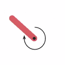
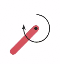
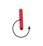
(a)	(b)	(c)

Figure 1: Various states of an inverted Pendulum. (a) and (b) are the intermediate unstable states; (c) is the final upright state which is desired.

II Methods

II-A The System

An inverted pendulum is a classical control problem having two degrees of freedom of motion and only one actuator to control its position. The motor is connected at the tip of the pendulum bar. The base joint of this bar is a free joint without any motor. The goal is to remain at zero angle (vertical position) with least rotational velocity and least effort. Some of the states of the pendulum is shown in Figure 1. The vertical upright position (c) is the desirable state for the system. The range of various input and output parameters for this simulation environment is provided in Table I. A simple python code to visualize the dynamic simulation of the system is provided in code listing II-A. The render option should be disabled during actual training to speed up the computation. Each episode involves 200 iteration steps. The total reward for an episode is the sum of individual rewards obtained at each of these steps. Since, no training is involved in this code, the total reward for each of these episodes will be a large negative number. The problem is considered solved if the average reward for an episode remains above -200 for a considerable amount of time (say, 50 episodes).

 import gym env = gym.make("Pendulum-v0") state_size = env.observation_space.shape action_size = env.action_space.shape upper_bound = env.action_space.high[0] lower_bound = env.action_space.low[0]  for ep in range(20):     state = env.reset()     done = False     ep_reward = 0     while not done:         env.render()         action = env.action_space.sample()         next_state, reward, done, _ = env.step(action)         ep_reward += reward         if done:             print(’Episode: {}, Reward: {}’.format(ep, ep_reward))             break env.close() Discretizing continuous states into discrete states

Variable Name	shape	Elements	Min	Max
Observation (state), $s$	(3,1)	$\cos{\theta}$	-1.0	1.0
		$\sin{\theta}$	-1.0	1.0
		$\dot{\theta}$	-8.0	8.0
Action, $a$	(1,)	Joint Effort	-2.0	2.0
Reward, $r$	(1,)	$-\theta^{2}+0.1\dot{\theta}^{2}+0.001a^{2}$	-16.273	0

TABLE I: Input-Output variables for ‘Pendulum-v0’ Gym Simulation Environment.

II-B Actor-Critic Model

The Pendulum problem is solved in this paper using an Actor-Critic model. In this model, an actor network is used to approximate the policy function $\mu_{\theta}(s)$ whereas a critic network is used to approximate the value function $V_{\phi}(s)$ or the function $Q_{\phi}(s,a)$. The actor-critic model allows one to implement separate training algorithm for the actor and the critic network and hence, provides greater flexibility compared to other models. The actor and critic class templates are shown in the code listings II-B and II-B respectively. The class template for the actor-critic agent is provided in listing II-B. Following the double DQN formalism [21], a separate target network is created for both DDPG actor and critic models which share the same weights as that of the actual models in the beginning. The weights of the target networks are updated slowly during the training process by using Polyak Averaging [13] as will be explained in the next section. The actor model for PPO algorithm returns mean and standard deviation of the policy distribution. The reinforcement learning agent initializes an actor model, a critic model and a buffer model. The buffer model is used for storing the experiences which will be used for training the DDPG agent. The agent provides two main functions - one for selecting policy (or action) and the other for training the agent. These functions are defined and explained in the later sections. In this paper, we only show the implementation of two main algorithms - DDPG and PPO. However, the same template could be used for incorporating other algorithms as well.

 class Actor:     def __init__(self, state_size, action_size):         self.model = self._build_net()         self.optim = tf.keras.optimizers.Adam(self.lr)          if self.flag == ’ddpg’:             self.target = self._build_net()             self.target.set_weights(self.model.get_weights())         elif self.flag == ’ppo’:             logstd = tf.Variable(np.zeros(shape=action_size, dtype=np.float32))             self.model.logstd = logstd             self.model.trainable_variables.append(logstd)      def _build_net(self):         pass      def __call__(self, state):         if self.flag == ’ddpg’:             return tf.squeeze(self.model(state))         elif self.flag == ’ppo’:             mean = tf.squeeze(self.model(state))             std = tf.squeeze(tf.exp(self.model.logstd))             return mean, std      def train(self):         if self.flag == ’ddpg’:             self.ddpg_train()         elif self.flag == ’ppo’:             self.ppo_train()      def update_target(self):         pass Class template for Actor Network

 class Critic:     def __init__(self, state_size, action_size):         self.model = _build_net()         self.optim = tf.keras.optimizers.Adam(self.lr)         if flag == ’ddpg’:             self.target = _build_net()             self.target.set_weights(self.model.get_weights())      def __call__(self, state):         return tf.squeeze(self.model(state))      def _build_net(self):         pass      def train(self):         if self.flag == ’ddpg’:             self.ddpg_train()         elif self.flag == ’ppo’:             self.ppo_train()      def update_target(self):         pass Class template for the Critic Network

 class Agent:     def __init__(self, state_size, action_size):         self.actor = Actor(state_size, action_size)         self.critic = Critic(state_size, action_size)         self.buffer = Buffer(max_size, tmax=1000)      def policy(self):         if self.flag == ’ddpg’:             self.ddpg_policy()         elif self.flag == ’ppo’:             self.ppo_policy()      def train(self):         if self.flag == ’ddpg’:             self.ddpg_train()             self.update_target() # update the target models         elif self.flag == ’ppo’:             self.ppo_train()             self.buffer.clear() # clear the buffer      def update_target(self):         if self.flag == ’ddpg’:             self.actor.update_target()             self.critic.update_target() Class template for the actor-critic agent

II-C Policy Gradient Methods

The policy gradient methods aims at learning a policy function $\pi_{\theta}=P(a|s)$ that maximizes an objective function $J(\theta)$ that computes the expected cumulative discounted rewards given by:

$$J(\theta)=\operatorname*{\mathbb{E}}\left[\sum_{t=0}^{\infty}r_{t+1}\right]$$ (1)

where $r_{t+1}=R(s_{t},a_{t})$ is the reward received by performing an action $a_{t}$ at state $s_{t}$. This can be expressed in terms of policy function $\pi_{\theta}(a|s)$ as follows:

$$J(\theta)=\operatorname*{\mathbb{E}}\left[\displaystyle\sum_{s\in\mathcal{S}}d^{\pi}(s)\sum_{a\in\mathcal{A}}\pi_{\theta}(a|s)Q^{\pi}(s,a)\right]$$ (2)

where $d^{\pi}(s)$ is the stationary distribution of Markov chain for $\pi_{\theta}$ given by

$$d^{\pi}(s)=\lim_{t\rightarrow\infty}P(s_{t}=s|s_{0},\pi_{\theta})$$ (3)

The policy parameter $\theta$ is updated using gradient ascent algorithm that aims to maximize the above objective function. The parameter update rule can be written as:

$$\theta=\theta+\eta\nabla_{\theta}J(\theta)$$ (4)

The gradient of the objective function is given by:

$$\nabla_{\theta}J(\theta)=\operatorname*{\mathbb{E}}\left[\sum_{t=0}^{\infty}Q^{\pi}(s_{t},a_{t})\nabla_{\theta}\log\pi_{\theta}(a_{t}|s_{t})\right]$$ (5)

In terms of advantage function $A^{\pi}(s_{t},a_{t})=Q^{\pi}(s_{t},a_{t})-V^{\pi}(s_{t})$, the above expression can be written as

$$\nabla_{\theta}J(\theta)=\operatorname*{\mathbb{E}}\left[\sum_{t=0}^{\infty}A^{\pi}(s_{t},a_{t})\nabla_{\theta}\log\pi_{\theta}(a_{t}|s_{t})\right]$$ (6)

The advantage function can be estimated from the value function estimates (details are available in [18]) by using the generalized advantage estimator given by the following equation:

$$\hat{A}_{t}=\sum_{l=0}^{\infty}(\gamma\lambda)^{l}\delta_{t+l}$$ (7)

where parameter $0\leq\lambda\leq 1$ controls the trade-off between bias and variance and $\delta_{t}$ represents the time delay error given by

$$\delta_{t}=r_{t}+\gamma V(s_{t+1})-V(s_{t})$$ (8)

 class Agent:     def compute_advantages(self, states, next_states, rewards, dones):         # inputs are tensors and outputs are numpy arrays         s_values = self.critic(states)         ns_values = self.critic(next_states)          adv = np.zeros(shape=(len(rewards), ))         returns = np.zeros(shape=(len(rewards), ))          discount = self.gamma         lmbda = self.lmbda         g = 0         returns_current = ns_values[-1]         for i in reversed(range(len(rewards))):             gamma = discount * (1. - dones[i])             td_error = rewards[i] + gamma * ns_values[i] - s_values[i]             g = td_error + gamma * lmbda * g             returns_current = rewards[i] + gamma * returns_current             adv[i] = g             returns[i] = returns_current         adv = (adv - np.mean(adv)) / (np.std(adv) + 1e-10)         return returns, adv Function definition for implementing generalized advantage estimates (GAE).

As explained in the previous subsection, the above optimization problem is solved in this paper by using an actor-critic method that combines the benefit of both value-based and policy-based methods. It consists of two models: Actor and Critic. The actor model is used to approximate the policy function $\pi_{\theta}(a|s)$ that computes an action for a given state while the critic model is used to evaluate this action by estimating the Q function $Q_{\phi}(s,a)$ or the value function $V_{\phi}(s)$.

The critic model updates the q-value function parameter $\phi$ of the action value $Q_{\phi}(s,a)$ or the state-value $V_{\phi}(s)$ function by using the time-delay error $\delta_{t}$ given by equation (8). The weight update rule for the critic may be written as:

$$\phi\leftarrow\phi+\alpha_{\phi}\delta_{t}\nabla_{\phi}Q_{\phi}(s,a)$$ (9)

On the other hand, the actor model updates the policy parameter $\theta$ for $\pi_{\theta}(a|s)$ so as to maximize the value function estimated by the critic. This weight update rule for the actor may be written as

$$\theta\leftarrow\theta+\alpha_{\theta}Q_{\phi}(s,a)\nabla_{\theta}\log\pi_{\theta}(a|s)$$ (10)

II-D Proximal Policy Optimization (PPO)

To improve the training stability, the parameter updates that result in large change in policy should be avoided. Trust Region Policy Optimization (TRPO) [17] ensures this by enforcing KL divergence constraint on the size of the policy update at each iteration. This is achieved by optimizing the following objective function:

$$J(\theta)=\operatorname*{\mathbb{E}}_{\mathbf{s}\sim\rho^{\pi_{\theta_{\text{old}}}},a\sim\pi_{\theta_{\text{old}}}}\left[\frac{\pi_{\theta}(a|s)}{\pi_{\theta_{\text{old}}}(a|s)}\hat{A}_{\theta_{\text{old}}}(s,a)\right]$$ (11)

subject to the trust region constraint given by:

$$\operatorname*{\mathbb{E}}_{\mathbf{s}\sim\rho^{\pi_{\theta_{\text{old}}}}}[D_{KL}(\pi_{\theta_{\text{old}}}(.|s)||\pi_{\theta}(.|s)]\leq\delta$$ (12)

where $\rho^{\pi_{\theta_{\text{old}}}}$ represents the state distribution under the old policy. The Proximal Policy Optimization (PPO) simplifies TRPO by using a clipped surrogate objective function while retaining similar performance.

Let us denote the probability ratio between new and old policy as:

$$r(\theta)=\frac{\pi_{\theta}(a|s)}{\pi_{\theta_{\text{old}}}(a|s)}$$ (13)

Then the objective function for TRPO becomes:

$$J^{TRPO}(\theta)=\operatorname*{\mathbb{E}}[r(\theta)\hat{A}_{\theta_{\text{old}}}(s,a)]$$ (14)

Maximizing this objective function without any restriction on distance between $\theta_{\text{old}}$ and $\theta$ would lead to instability with large parameter updates and big policy ratios. PPO avoids this by forcing $r(\theta)$ to stay within a small interval around 1, $[1-\epsilon,1+\epsilon]$, where $\epsilon$ is a hyperparameter. The modified cost function maximized in PPO is given by

$$J^{CLIP}(\theta) =\operatorname*{\mathbb{E}}[\min(r(\theta)\hat{A}_{\theta_{\text{old}}}(s,a),$$

$$\quad\quad\text{clip}(r(\theta),1-\epsilon,1+\epsilon)\hat{A}_{\theta_{\text{old}}}(s,a))]$$

$$=\mathscr{L}(s,a,\theta_{\text{old}},\theta)$$ (15)

While applying PPO to an actor-critic kind of model, the above objective function is augmented with an error term on the value estimation and an entropy term as shown below for better performance:

$$J^{CLIP}(\theta)=\operatorname*{\mathbb{E}}[J^{CLIP}(\theta)-c_{1}(V_{\theta}(s)-V_{\text{target}})^{2}\\ +c_{2}H(s,\pi_{\theta}(.))]$$ (16)

The algorithm for the PPO-Clip method is provided in the algorithm listing 1. It is also possible to impose this constraint by including a penalty term on the KL divergence term $D_{KL}(\theta||\theta_{\text{old}})$ in the objective function which will ensure that the new policy does not deviate too much from the current policy. Hence the policy optimization problem given in equation (11) and (12) may be rewritten as:

$$\operatorname*{\scriptsize\mathbf{maximize}}_{\theta}\left(\operatorname*{\mathbb{E}}[\frac{\pi_{\theta}(a|s)}{\pi_{\theta_{\text{old}}}(a|s)}\hat{A}]-\beta\operatorname*{\mathbb{E}}[D_{KL}(\theta||\theta_{\text{old}})]\right)$$ (17)

where $\beta$ controls the weight of the penalty which itself can be adaptively varied as the training progresses. The resulting PPO algorithm is shown in Algorithm listing 2.

Algorithm 1 PPO-Clip Algorithm

0: initial policy parameters $\theta_{0}$, initial value function parameters $\phi_{0}$

1: for $k=0,1,2,\dots$ do

2:    Collect a set of trajectories $\mathscr{D}_{k}=\{\tau_{i}\}$ by running policy $\pi_{k}=\pi(\theta_{k})$ in the environment.

3:    Compute rewards-to-go $\hat{R}_{k}$

4:    Compute advantage estimates $\hat{A}_{k}$ based on the current value function $V(\phi_{k})$

5:    Update the policy by maximizing the PPO-Clip objective via stochastic gradient ascent:

$$\theta_{k+1}=\arg\max_{\theta}\frac{1}{|\mathscr{D}_{k}|T}\sum_{\tau\in\mathscr{D}_{k}}\sum_{t=0}^{T}\\ \min\left(r(\theta)A^{\pi_{k}}(s_{t},a_{t}),g(\epsilon,A^{\pi_{k}}(s_{t},a_{t}))\right)$$ (18)

where

$$g(\epsilon,a)=\left\{\begin{array}[]{l}(1+\epsilon)A\ \text{if}\ A\geq 0\\ (1-\epsilon)A\ \text{if}\ A<0\end{array}\right.$$

6:    Update value function to minimize the following error function by using gradient descent algorithm:

$$\phi_{k+1}=\arg\min_{\phi}\frac{1}{|\mathscr{D}_{k}|T}\sum_{\tau\in\mathscr{D}_{k}}\sum_{t=0}^{T}\left(V_{\phi}(s_{t})-\hat{R}_{t}\right)^{2}$$ (19)

7: end for

Algorithm 2 PPO with Adaptive KL Penalty

0: initial policy parameter $\theta_{0}$, initial value parameter $\phi_{0}$, initial KL penalty $\beta_{0}$, target KL-divergence $\delta$

1: for $k=0,1,2,\dots$ do

2:    Collect a set of partial trajectories $\mathscr{D}_{k}$ on policy $\pi=\pi(\theta_{k})$.

3:    Estimate Advantage $\hat{A}_{k}$ based on current value function $V(\phi_{k})$

4:    Compute policy update

$$\theta_{k+1}=\arg\max_{\theta}\mathscr{L}_{\theta_{k}}(\theta)-\beta_{k}\bar{D}_{KL}(\theta||\theta_{k})$$

by taking k steps of mini-batch SGD

5:    if $\bar{D}_{KL}(\theta_{k+1}||\theta_{k})\geq 1.5\delta$ then

6:       $\beta_{k+1}=2\beta_{k}$

7:    else if $\bar{D}_{KL}(\theta_{k+1}||\theta_{k})\leq 1.5/\delta$ then

8:       $\beta_{k+1}=\beta_{k}/2$

9:    end if

10: end for

The corresponding function definitions required for implementing PPO algorithm is provided in listings 2 and 2 respectively. The adaptive KL penalty method is enabled by using the value ‘penalty’ and the clip method is enabled by using the value ‘clip’ for the flag ‘method’ in the actor class object. The experiences are first collected in a buffer and then used for computing advantages by using the Generalized Advantage Estimator (GAE) equation (7). These experiences and estimates are then split into a number of mini-batches which are then used for training actor and critic networks for a certain number of epochs. The target values are the cumulative discounted reward computed using a low pass filter function available with ‘scipy.signal’ module. The ‘tensorflow_probability’ module is used for computing likelihood ratio, KL divergence and the action probability distribution. The buffer is cleared or emptied after each training step. This makes the PPO algorithm an on-policy method that uses the current experiences to train the model.

 import tensorflow_probability as tfp class Actor:     def ppo_train(self, state_batch, action_batch, advantages, old_pi):         with tf.GradientTape() as tape:             mean = tf.squeeze(self.model(state_batch))             std = tf.squeeze(tf.exp(self.model.logstd))             pi = tfp.distributions.Normal(mean, std)             ratio = tf.exp(pi.log_prob(tf.squeeze(action_batch)) -                            old_pi.log_prob(tf.squeeze(action_batch)))             surr = ratio * advantages  # surrogate function             kl = tfp.distributions.kl_divergence(old_pi, pi)             self.kl_value = tf.reduce_mean(kl)             if self.method == ’penalty’:  # ppo-penalty method                 actor_loss = -(tf.reduce_mean(surr - self.lam * kl))                 # self.update_lambda()             elif self.method == ’clip’:  # ppo-clip method                 actor_loss = - tf.reduce_mean(                     tf.minimum(surr, tf.clip_by_value(ratio,\                             1. - self.epsilon, 1. + self.epsilon) * advantages))             actor_weights = self.model.trainable_variables          # outside gradient tape         actor_grad = tape.gradient(actor_loss, actor_weights)         self.optimizer.apply_gradients(zip(actor_grad, actor_weights))          return actor_loss.numpy(), self.kl_value.numpy()   class Critic:      def ppo_train(self, state_batch, disc_rewards):         with tf.GradientTape() as tape:             critic_weights = self.model.trainable_variables             critic_value = tf.squeeze(self.model(state_batch))             critic_loss = tf.math.reduce_mean(tf.square(disc_rewards - critic_value))         critic_grad = tape.gradient(critic_loss, critic_weights)         self.optimizer.apply_gradients(zip(critic_grad, critic_weights)) Training Actor and Critic using PPO Algorithm

 class Agent:     def ppo_train(self, training_epochs=20, tmax=10000):         # make sure to have enough samples in buffer for training         if tmax is not None and len(self.buffer) < tmax:             return 0, 0, 0          n_split = len(self.buffer) // self.batch_size         n_samples = n_split * self.batch_size          s_batch, a_batch, r_batch, ns_batch, d_batch = \             self.buffer.get_samples(n_samples)          s_batch = tf.convert_to_tensor(s_batch, dtype=tf.float32)         a_batch = tf.convert_to_tensor(a_batch, dtype=tf.float32)         r_batch = tf.convert_to_tensor(r_batch, dtype=tf.float32)         ns_batch = tf.convert_to_tensor(ns_batch, dtype=tf.float32)         d_batch = tf.convert_to_tensor(d_batch, dtype=tf.float32)          # compute GAE and discounted returns         target_values, advantages = self.compute_advantages(s_batch, \                                                 ns_batch, r_batch, d_batch)          advantages = tf.convert_to_tensor(advantages, dtype=tf.float32)         disc_sum_reward = tf.convert_to_tensor(                 disc_sum_reward, dtype=tf.float32)          # current policy         mean, std = self.actor(s_batch)         pi = tfp.distributions.Normal(mean, std)          s_split = tf.split(s_batch, n_split)         a_split = tf.split(a_batch, n_split)         dr_split = tf.split(disc_sum_reward, n_split)         adv_split = tf.split(advantages, n_split)         indexes = np.arange(n_split, dtype=int)          a_loss_list = []         c_loss_list = []         kld_list = []         np.random.shuffle(indexes)         for _ in range(training_epochs):             for i in indexes:                 old_pi = pi[i*self.batch_size: (i+1)*self.batch_size]                  # update actor                 a_loss, kld = self.actor.ppo_train(s_split[i],                         a_split[i], adv_split[i], old_pi)                 a_loss_list.append(a_loss)                 kld_list.append(kld)                  # update critic                 c_loss_list.append(                         self.critic.ppo_train(s_split[i], dr_split[i]))              # update lambda after each epoch             if self.method == ’penalty’:                 self.actor.update_beta()          actor_loss = np.mean(a_loss_list)         critic_loss = np.mean(c_loss_list)         mean_kld = np.mean(kld_list)          # clear the buffer  -- this is important         self.buffer.clear()          return actor_loss, critic_loss, mean_kld PPO training algorithm for the Agent

II-E Deep Deterministic Policy Gradient (DDPG) Algorithm

Deep Deterministic Policy Gradient (DDPG) algorithm [9] concurrently learns a Q-function and a policy. It uses off-policy data and the Bellman equation to learn the Q-function and then learns a policy by maximizing the Q-function through a gradient ascent algorithm. This allows DDPG to apply deep Q-learning to continuous action spaces.

The Q-learning in DDPG is performed by minimizing the following mean squared bellman error (MBSE) loss with stochastic gradient descent:

$$L(\phi,\mathscr{D})=\operatorname*{\mathbb{E}}_{(s,a,r,s^{\prime},d)\sim\mathscr{D}}\biggl{[}\biggl{(}Q_{\phi}(s,a)-\\ (r+\gamma(1-d)Q_{\phi_{\text{targ}}}(s^{\prime},\mu_{\theta_{\text{targ}}}(s^{\prime})))\biggr{)}^{2}\biggr{]}\\ =\operatorname*{\mathbb{E}}_{(s,a,r,s^{\prime},d)\sim\mathscr{D}}[Q_{\phi}(s,a)-y(r,s^{\prime},d)]$$ (20)

where $\mu_{\theta_{\text{targ}}}$ is the target policy, $Q_{\phi_{\text{targ}}}$ is the target Q network and $y(r,s^{\prime},d)$ is the target critic value required for training the Q network.

The policy learning in DDPG aims at learning a deterministic policy $\mu_{\theta}(s)$ which gives action that maximizes $Q_{\phi}(s,a)$. Since the action space is continuous, it is assumed that the Q function is differentiable with respect to action. The policy parameters $\theta$ are updated by performing gradient ascent to solve the following optimization problem:

$$\max_{\theta}\operatorname*{\mathbb{E}}_{s\sim\mathscr{D}}[Q_{\phi}(s,\mu_{\theta}(s))]$$ (21)

The parameters of the target networks are updated slowly compared to the main network by using Polyak Averaging [13] as shown below:

$$\phi_{\text{targ}} \leftarrow \rho\phi_{\text{targ}}+(1-\rho)\phi$$

$$\theta_{\text{targ}} \leftarrow \theta\phi_{\text{targ}}+(1-\rho)\theta$$

where $0\leq\rho\leq 1$ is a hyper parameter.

The pseudocode for DDPG algorithm is provided in the Algorithm table 3 and its python implementation is provided in listing II-E. The DDPG agent samples a batch of experiences from the replay buffer and uses it to train the actor and critic networks. As explained above, the actor implements gradient ascent algorithm by using a negative of the gradient term computed using Tensorflow’s ‘GradientTape’ utility. The critic, on the other hand, learns by applying gradient descent to minimize the time-delay Q-function error.

Algorithm 3 DDPG Algorithm

1: input: initial policy parameter $\theta$, initial Q-function parameters $\phi$, empty replay buffer $\mathscr{D}$.

2: set target parameters equal to the main parameters: $\theta_{\text{targ}}\leftarrow\theta$, $\phi_{\text{targ}}\leftarrow\phi$.

3: repeat

4:    Observe state $s$ and select action $a=\text{clip}(\mu_{\theta}(s)+\epsilon,a_{Low},a_{High})$, where $\epsilon\sim\mathscr{N}$.

5:    Execute the action $a$ in the environment and obtain next state $s^{\prime}$, reward $r$, done signal $d$ to indicate if it is a terminal state.

6:    Store $(s,a,r,s^{\prime},d)$ in the replay buffer $\mathscr{D}$

7:    if $s^{\prime}$ is terminal, reset the environment.

8:    if it’s time to update then

9:       for for a certain number of steps do

10:          Randomly sample a batch of transitions $B={(s,a,r,s^{\prime},d)}$ from $\mathscr{D}$.

11:          Compute targets: $y(r,s^{\prime},d)=r+\gamma(1-d)Q_{\phi_{\text{targ}}}(s^{\prime},\mu_{\theta_{\text{target}}}(s^{\prime}))$

12:          Update Q function by applying one step of gradient descent using $\displaystyle\nabla_{\phi}\frac{1}{|B|}\sum_{(s,a,r,s^{\prime},d)\in B}(Q_{\phi}(s,a)-y(r,s^{\prime},d))^{2}$

13:          Update policy by one step of gradient ascent using $\displaystyle\nabla_{\theta}\frac{1}{|B|}\sum_{s\in B}Q_{\phi}(s,\mu_{\theta}(s))$

14:          Update target networks using Polyak Averaging given by equations (II-E)

15:       end for

16:    end if

17: until convergence

 class Actor:     def ddpg_train(self, state_batch, critic):         with tf.GradientTape() as tape:             actor_weights = self.model.trainable_variables             actions = self.model(state_batch)             critic_value = critic.model([state_batch, actions])             # -ve value is used to maximize value function             actor_loss = -tf.math.reduce_mean(critic_value)         actor_grad = tape.gradient(actor_loss, actor_weights)         self.optimizer.apply_gradients(zip(actor_grad, actor_weights))  class Critic:     def ddpg_train(self, state_batch, action_batch, reward_batch,                                     next_state_batch, actor):         with tf.GradientTape() as tape:             critic_weights = self.model.trainable_variables             target_actions = actor.target(next_state_batch)             target_critic = self.target([next_state_batch, target_actions])             y = reward_batch + self.gamma * target_critic             critic_value = self.model([state_batch, action_batch])             critic_loss = tf.math.reduce_mean(tf.square(y - critic_value))         critic_grad = tape.gradient(critic_loss, critic_weights)         self.optimizer.apply_gradients(zip(critic_grad, critic_weights))  class Agent:     def ddpg_train(self):         # sample from stored memory         state_batch, action_batch, reward_batch,\                         next_state_batch = self.buffer.sample()         # train actor and critic models         self.actor.ddpg_train(state_batch, self.critic)         self.critic.ddpg_train(state_batch, action_batch, reward_batch,                           next_state_batch, self.actor) Function Definitions for implementing DDPG algorithm

III Other Implementation Details

The main function for implementing these two algorithms is shown in the listing III. The main training loop involves the following steps: (1) Compute action as per the current agent policy (2) Obtain reward from the environment by executing the above action, (3) Store this experience tuple $(s,a,r,s^{\prime},d)$ in a buffer. (4) Use this experience to the train the agent. The environment is reset once the terminal state is reached indicating the end of the current episode. The PPO algorithm is an on-policy method and hence, the experiences in the buffer are discarded after each training iteration. On the other hand, DDPG is an off-policy method that uses a sample of past experiences to train the agent.

 import gym if __name__ == ’__main__’:     # start open/AI GYM environment     env = gym.make(’Pendulum-v0’)     # Create an Actor-Critic Agent     agent = Agent(state_size, action_size, batch_size=128,                          upper_bound=upper_bound, ...)     state_size = env.observation_space.shape     action_size = env.observation_space.shape     upper_bound = env.action_space.high[0]     # training loop     ep_reward_list = []     for ep in range(MAX_EPISODES):         state = env.reset()         ep_reward = 0         while True:             # take action based on current policy             action = agent.policy(state)             # gather rewards from the environment             next_state, reward, done, _ = env.step(action)             # collect experiences             agent.buffer.record(state, action, reward, next_state, done)             ep_reward += reward             # train             agent.train()             state = next_state             if done:                 ep_reward_list.append(ep_reward)                 break         if np.mean(ep_reward_list[-40:]) > -200:             print(’Problem is solved in {} episodes’.format(ep))             break     env.close() Main Python File

 class Agent:     def ppo_policy(self, state):         tf_state = tf.expand_dims(tf.convert_to_tensor(state), 0)         mean, std = self.actor(tf_state)         pi = tfp.distributions.Normal(mean, std)         # sample from the current policy distribution         action = pi.sample(sample_shape=self.action_size)         valid_action = tf.clip_by_value(action,                 -self.upper_bound, self.upper_bound)         return valid_action.numpy()      def ddpg_policy(self, state):         tf_state = tf.expand_dims(tf.convert_to_tensor(state), 0)         # obtain action by using deterministic policy         sampled_action = tf.squeeze(self.actor.model(tf_state))         noise = self.noise_object()         # Add noise to the action         sampled_action = sampled_action.numpy() + noise         # Make sure that the action is within bounds         valid_action = np.clip(sampled_action,                 self.lower_bound, self.upper_bound)         return valid_action.numpy() Agent policy function for generating action for a given state

The agent policy used for generating action for a given state is shown in listing III. The actor in DDPG uses a noisy version of a deterministic policy to generate actions for a given state. On the other hand, the actor in PPO draws an action from a policy distribution.

 from keras import layers class Critic:     def _build_net(self):         state_input = layers.Input(shape=self.state_size)         out = layers.Dense(64, activation="relu")(state_input)         out = layers.Dense(64, activation="relu")(out)         out = layers.Dense(64, activation="relu")(out)         net_out = layers.Dense(1)(out)         # Outputs single value for give state-action         model = tf.keras.Model(inputs=state_input, outputs=net_out)         model.summary()         return model  class Actor:     def _build_net(self):         last_init = tf.random_uniform_initializer(minval=-0.003, maxval=0.003)         state_input = layers.Input(shape=self.state_size)         l = layers.Dense(128, activation=’relu’)(state_input)         l = layers.Dense(64, activation=’relu’)(l)         l = layers.Dense(64, activation=’relu’)(l)         net_out = layers.Dense(self.action_size[0], activation=’tanh’,                                kernel_initializer=last_init)(l)         net_out = net_out * self.upper_bound         model = keras.Model(state_input, net_out)         model.summary()         return model Deep Neural Network for Actor and Critic Models

Each of the actor and critic models use a deep network to estimate the policy and value functions respectively. Tensorflow’s Keras APIs are used to create these deep networks as shown in the code listing III. The actor uses a sequential 128-64-64-1 multiple layer perceptron (MLP) network to estimate the policy function $\mu_{\theta}$. Similarly, the critic model uses a sequential 64-64-64-1 MLP network to estimate the value function $V_{\phi}(s)$ for given state input. It is to be noted that the action and states are continuous floating point values for the current problem.

IV Experiments and Results

The full source codes for the implementations are available on the GitHub [6] for the convenience of readers. These codes are implemented in Python 3.x by using Tensorflow 2.x and Keras APIs. TF 2.0 uses eager implementation by default and hence provides cleaner interface compared to TF 1.0 that uses placeholders and sessions instead. These codes could be easily implemented on various online GPU cloud platforms such as Google Colab [3] and Kaggle [5].

The training results for DDPG algorithm is shown in Figure 2. It shows the average reward of last 40 episodes against the training episodes. The problem is considered solved when this average reward exceeds -200. As one can see in this figure, the DDPG algorithm solves the problem in about 50-60 episodes. The complete execution takes about a couple of hours on Google Colab.

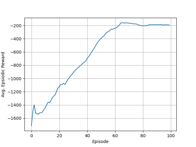
Figure 2: Training performance with DDPG algorithm. It solves the problem within 50-60 episodes.

The results for PPO algorithm is shown in Figure 3-4. The Figure 3 shows the average episodic reward of a given season as the training proceeds. Each season consists of about 50 episodes. The problem is considered solved if the season score exceeds a reward of -200. The actor and critic losses are shown in Figure 4(a)-(b). The critic loss decreases monotonically indicating that the network is able to minimize the time-delay error of the Q-network. The KL-Divergence between the old policy and the new policy is shown in Figure 4(c). It shows that the KL-divergence value remains close to the KL target value of 0.01. The variation of the KL penalty factor $\beta$ value in adaptive KL penalty method (Algorithm 2) is shown in Figure 4(d).

The hyper parameters used for these two algorithms is shown in Table II. The number of samples used during each training iteration is about 10,000 as each episode has about 200 time-steps. The content of the buffer is discarded after each training iteration. On the other hand, the replay buffer of DDPG algorithm has a maximum size of 20,000 and the old experiences are removed as the buffer gets filled over time. Each training step in PPO involves multiple training epochs each of which uses a mini-batch of the experiences stored in the buffer.

PPO		DDPG
Actor learning rate, $\alpha_{a}$	1e-4	$\alpha_{a}$	1e-3
Critic learning rate, $\alpha_{c}$	2e-4	$\alpha_{c}$	2e-3
Discount factor, $\gamma$	0.9	$\gamma$	0.99
Discount factor in GAE, $\lambda$	0.95	Polyak averaging factor, $\tau$	0.005
KL penalty factor, $\beta$	0.5
Clip factor, $\epsilon$	0.2
KL Target	0.01
Training epochs	20
Batch size	200	Batch size	64
Buffer Size, $t_{\text{max}}$	10,000	Replay buffer size	20,000

TABLE II: Hyper-parameters used for implementing PPO and DDPG Algorithms

Figure 3: Training Performance of PPO Algorithm. Season score is the average episodic reward for a season. Each season consists of 50 episodes.

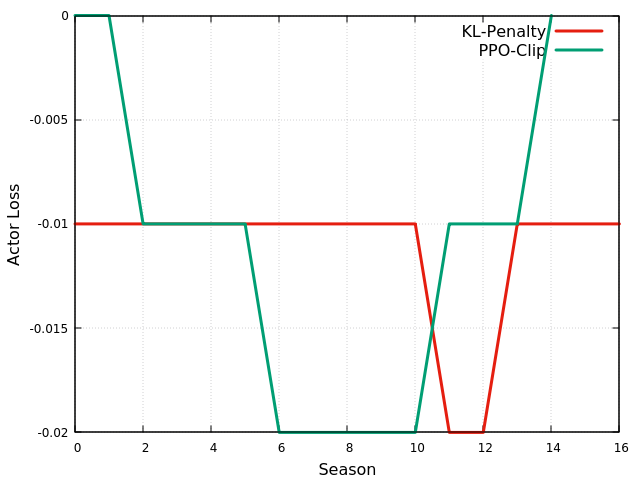
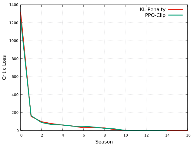
(a)	(b)
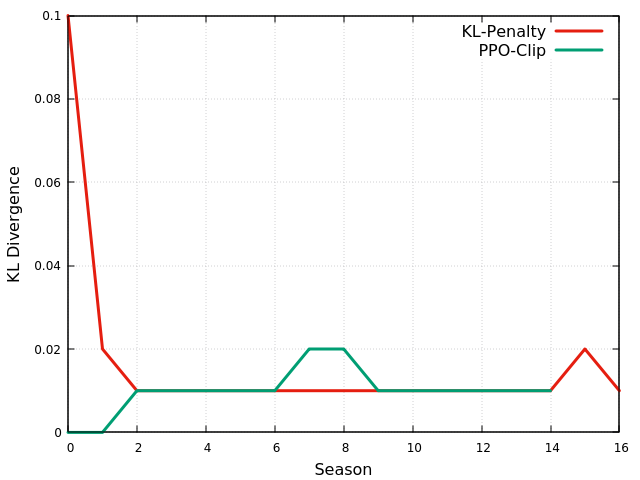
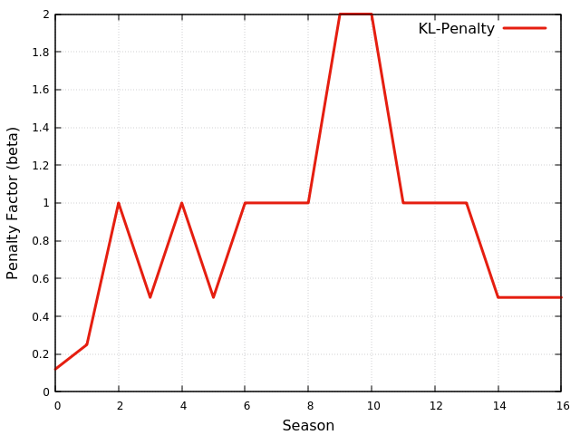
(c)	(d)

Figure 4: Training Performance of PPO algorithms: (a) Actor loss (b) Critic Loss (c) KL Divergence and (d) Penalty factor ($\beta$)

Discussion

It may seem that DDPG is faster than PPO in this case. However, making such direct comparison may not be fair. It is to be noted that DDPG is an off-policy method while PPO is an on-policy method. Secondly, PPO provides more efficient training compared to DDPG for more complex problems such Kuka-Grasp [14] or roboschool [15]. Third, there are more efficient versions of actor-critic model such as A3C [1] where data collection and training can be carried out by multiple workers working in parallel. Finally, the intention of this paper is not to make any comparison between these two algorithms. The objective is to understand the underlying concepts behind these algorithms and see them working on a simpler problem.

V Conclusion

This paper provides the details of implementing two main policy gradient methods, namely, DDPG and PPO to solve the OpenAI/Gym’s inverted pendulum problem. The mathematical background of these two methods are discussed along with their implementation using Python programming. The problem is solved by using an actor-critic model where the actor is used to estimated the agent’s policy which is evaluated using the critic network. The information provided in this paper will be useful for beginners who would like to acquire advanced understanding of reinforcement learning concepts in minimum time. The actual code is made available on GitHub for the convenience of readers and can be easily implemented using online GPU platforms such as Google Colab [3] and Kaggle [5]. Results show that the DDPG algorithm takes around 50-60 episodes to solve the problem while the PPO takes around 15-20 seasons (about 1000 episodes) for the same.

References

- [1] M. Babaeizadeh, I. Frosio, S. Tyree, J. Clemons, and J. Kautz. Ga3c: Gpu-based a3c for deep reinforcement learning. CoRR abs/1611.06256, 2016.
- [2] A. G. Barto. Reinforcement learning and dynamic programming. In Analysis, Design and Evaluation of Man–Machine Systems 1995, pages 407–412. Elsevier, 1995.
- [3] Google Colaboratory. Online interactive gpu cloud platform for implementing deep learning algorithms. https://colab.research.google.com.
- [4] S. D. Holcomb, W. K. Porter, S. V. Ault, G. Mao, and J. Wang. Overview on deepmind and its alphago zero ai. In Proceedings of the 2018 international conference on big data and education, pages 67–71, 2018.
- [5] Kaggle. Online gpu cloud platform for implementing deep learning algorithms. https://www.kaggle.com.
- [6] S. Kumar. Reinforcement learning codes for pendulum gym environment. https://github.com/swagatk/RL-Projects-SK/tree/master/src/Pendulum.
- [7] S. Kumar. Balancing a cartpole system with reinforcement learning – a tutorial, 2020.
- [8] Y. Li. Deep reinforcement learning: An overview. arXiv preprint arXiv:1701.07274, 2017.
- [9] T. P. Lillicrap, J. J. Hunt, A. Pritzel, N. Heess, T. Erez, Y. Tassa, D. Silver, and D. Wierstra. Continuous control with deep reinforcement learning. arXiv preprint arXiv:1509.02971, 2015.
- [10] V. Mnih, K. Kavukcuoglu, D. Silver, A. Graves, I. Antonoglou, D. Wierstra, and M. Riedmiller. Playing atari with deep reinforcement learning. arXiv preprint arXiv:1312.5602, 2013.
- [11] V. Mnih, K. Kavukcuoglu, D. Silver, A. A. Rusu, J. Veness, M. G. Bellemare, A. Graves, M. Riedmiller, A. K. Fidjeland, G. Ostrovski, et al. Human-level control through deep reinforcement learning. nature, 518(7540):529–533, 2015.
- [12] J. Peters and S. Schaal. Policy gradient methods for robotics. In 2006 IEEE/RSJ International Conference on Intelligent Robots and Systems, pages 2219–2225. IEEE, 2006.
- [13] B. T. Polyak and A. B. Juditsky. Acceleration of stochastic approximation by averaging. SIAM journal on control and optimization, 30(4):838–855, 1992.
- [14] PyBullet. Kuka grasp simulation environment. https://github.com/bulletphysics/bullet3.
- [15] RoboSchool. Open-source software for robot simulation, integrated with openai/gym. https://openai.com/blog/roboschool/.
- [16] T. Schaul, J. Quan, I. Antonoglou, and D. Silver. Prioritized experience replay. arXiv preprint arXiv:1511.05952, 2015.
- [17] J. Schulman, S. Levine, P. Abbeel, M. Jordan, and P. Moritz. Trust region policy optimization. In International conference on machine learning, pages 1889–1897. PMLR, 2015.
- [18] J. Schulman, P. Moritz, S. Levine, M. Jordan, and P. Abbeel. High-dimensional continuous control using generalized advantage estimation. arXiv preprint arXiv:1506.02438, 2015.
- [19] M. Sewak. Deep q network (dqn), double dqn, and dueling dqn. In Deep Reinforcement Learning, pages 95–108. Springer, 2019.
- [20] R. S. Sutton and A. G. Barto. Reinforcement learning: An introduction. MIT press, 2018.
- [21] H. Van Hasselt, A. Guez, and D. Silver. Deep reinforcement learning with double q-learning. In Proceedings of the AAAI Conference on Artificial Intelligence, volume 30, 2016.
- [22] S. Wang, D. Jia, and X. Weng. Deep reinforcement learning for autonomous driving. arXiv preprint arXiv:1811.11329, 2018.
- [23] C. J. Watkins and P. Dayan. Q-learning. Machine learning, 8(3-4):279–292, 1992.