QuaSiMo: A Composable Library to Program Hybrid Workflows for Quantum Simulation

Abstract.

We present a composable design scheme for the development of hybrid quantum/classical algorithms and workflows for applications of quantum simulation. Our object-oriented approach is based on constructing an expressive set of common data structures and methods that enable programming of a broad variety of complex hybrid quantum simulation applications. The abstract core of our scheme is distilled from the analysis of the current quantum simulation algorithms. Subsequently, it allows a synthesis of new hybrid algorithms and workflows via the extension, specialization, and dynamic customization of the abstract core classes defined by our design. We implement our design scheme using the hardware-agnostic programming language QCOR into the QuaSiMo library. To validate our implementation, we test and show its utility on commercial quantum processors from IBM and Rigetti, running some prototypical quantum simulations.

1. Introduction

Quantum simulation is an important use case of quantum computing for scientific computing applications. Whereas numerical calculations of quantum dynamics and structure are staples of modern scientific computing, quantum simulation represents the analogous computation based on the principles of quantum physics. Specific applications are wide-ranging and include calculations of electronic structure (aspuru2005simulated, ; whitfield2011simulation, ; cao2019quantum, ; mcardle2020quantum, ), scattering (yeter2020scattering, ), dissociation (o2016scalable, ), thermal rate constants (lidar1999calculating, ), materials dynamics (bassman2020towards, ), and response functions (kosugi2020linear, ).

Presently, this diversity of quantum simulation applications is being explored with quantum computing despite the limitations on the fidelity and capacity of quantum hardware (PhysRevLett.124.230501, ; cirstoiu2020variational, ; google2020hartree, ). These applications are tailored to such limitations by designing algorithms that can be tuned and optimized in the presence of noise or model representations that can be reduced in dimensionality. Examples include variational methods such as the variational quantum eigensolver (VQE) (mcclean2016theory, ; romero2018strategies, ; grimsley2019adaptive, ; tang2019qubit, ), quantum approximate optimization algorithm (QAOA) (farhi2014quantum, ), quantum imaginary time evolution (QITE) (motta2019determining, ), and quantum machine learning (QML) among others.

The varied use of quantum simulation raises concerns for efficient and effective programming of these applications. The current diversity in quantum computing hardware and low-level, hardware-specific languages imposes a significant burden on the application user. For instance, IBM provides Aqua (Qiskit-Aqua, ), which is part of the Qiskit framework, targeting high-level quantum applications such as chemistry and finance. The emphasis of Aqua is on providing robust implementations of quantum algorithms, yet the concept of reusable and extensible workflows, especially for quantum simulations, is not formally supported. The user usually has to implement custom workflows from lower-level constructs, such as circuits and operators, available in Qiskit Terra (Qiskit-Terra, ). Similarly, Tequila (kottmann2020tequila, ) is another Python library that provides commonly-used functionalities for quick prototyping of variational-type quantum algorithms. Orquestra (Orquestra, ), a commercially-available solution from Zapata, on the other hand, orchestrates quantum application workflows as black-box phases, thus requires users to provide implementations for each phase.

The lack of a common workflow for applications of quantum simulation hinders broader progress in testing and evaluation of such hardware. A common, reusable and extensible programming workflow for quantum simulation would enable broader adoption of these applications and support more robust testing by the quantum computing community.

In this contribution, we address development of common workflows to unify applications of quantum simulation. Our approach constructs common data structures and methods to program varying quantum simulation applications, and we leverage the hardware-agnostic language QCOR and programming framework XACC to implement these ideas. We demonstrate these methods with example applications from materials science and chemistry, and we discuss how to extend these workflows to experimental validation of quantum computation advantage, in which numerical simulations can benchmark programs for small-sized models (kandala2017hardware, ; hempel2018quantum, ; mccaskey2019quantum, ; google2020hartree, ; yeter2020practical, ).

Upon release of the QuaSiMo library, we became aware of the additional application modules available to the Qiskit framework which share a number of features with our proposed composable workflow design. In particular, the Qiskit Nature module (qiskit-nature, ) introduces new concepts to model and solve quantum simulation problems, and reiterates the need for modular, domain-specific, and workflow-driven quantum application builders, which the QuaSiMo work addresses. The key differentiators for our work lie in the performance and extensibility of the implementation. Since QuaSiMo is developed on top of the C++ QCOR compiler infrastructure, it can take advantage of optimal performance for classical computing components of the workflow, such as circuit construction (qcor2, ) or post-processing. Moreover, the plugin-based extension model of QuaSiMo is distinct from that of Qiskit Nature. Rather than requiring new extensions being imported, QuaSiMo puts forward a common interface for all of its extension points (osgi, ), and therefore enables the development of portable user applications w.r.t. the underlying library implementation.

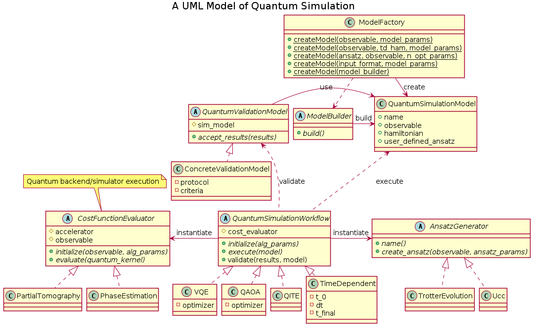
Figure 1. The class UML diagram of the quantum simulation application. The fully typed version is provided separately (see (paper_repo, )).

2. Software Architecture

Cloud-based access to quantum computing naturally differentiates programming into conventional and quantum tasks (britt2017high, ; xacc1, ). The resulting hybrid execution model yields a loosely integrated computing system by which common methods have emerged for programming and data flow. We emphasize this concept of workflow to organize programming applications for quantum simulation.

Figure 1 shows the blueprint of our Quantum Simulation Modeling (QuaSiMo) library. The programming workflow is defined by a QuantumSimulationWorkflow concept which encapsulates the hybrid quantum-classical procedures pertinent to a quantum simulation, e.g., VQE, QAOA, or dynamical quantum simulation. A quantum simulation workflow exposes an execute method taking as input a QuantumSimulationModel object representing the quantum model that needs to be simulated. This model captures quantum mechanical observables, such as energy, spin magnetization, etc., that we want the workflow to solve or simulate for. In addition, information about the system Hamiltonian, if different from the observable operator of interest, and customized initial quantum state preparation can also be specified in the QuantumSimulationModel.

By separating the quantum simulation model from the simulation workflow, our object-oriented design allows the concrete simulation workflow to simulate rather generic quantum models. This design leverages the ModelFactory utility, implementing the object-oriented factory method pattern. A broad variety of input mechanisms, such as those provided by the QCOR infrastructure or based on custom interoperability wrappers for quantum-chemistry software, can thus be covered by a single customizable polymorphic model. For additional flexibility, the last createModel factory method overload accepts a polymorphic builder interface ModelBuilder the implementations of which can build arbitrarily composed QuantumSimulationModel objects.

QuantumSimulationWorkflow is the main extension point of our QuaSiMo library. Built upon the CppMicroServices framework conforming to the Open Services Gateway Initiative (OSGi) standard (marples2001open, ), QuaSiMo allows implementation of a new quantum workflow as a plugin loadable at runtime. At the time of this writing, we have developed the QuantumSimulationWorkflow plugins for the VQE, QAOA, QITE, and time-dependent simulation algorithms, as depicted in Fig. 1. All these plugins are implemented in the QCOR language (qcor1, ; qcor2, ) using the externally-provided library routines.

At its core, a hybrid quantum-classical workflow is a procedural description of the quantum circuit composition, pre-processing, execution (on hardware or simulators), and post-processing. To facilitate modularity and reusability in workflow development, we put forward two concepts, AnsatzGenerator and CostFunctionEvaluator. AnsatzGenerator is a helper utility used to generate quantum circuits based on a predefined method such as the Trotter decomposition (trotter1959product, ; suzuki1976generalized, ) or the unitary coupled-cluster (UCC) ansatz (barkoutsos2018quantum, ). CostFunctionEvaluator automates the process of calculating the expectation value of an observable operator. For example, a common approach is to use the partial state tomography method of adding change-of-basis gates to compute the operator expectation value in the Z basis. Given the CostFunctionEvaluator interface, quantum workflow instances can abstract away the quantum backend execution and the corresponding post-processing of the results. This functional decomposition is particularly advantageous in the NISQ regime since one can easily integrate the noise-mitigation techniques, e.g., the verified quantum phase estimation protocol (o2020error, ), into the QuaSiMo library, which can then be used interchangeably by all existing workflows.

Finally, our abstract QuantumSimulationWorkflow class also exposes a public validate method accepting a variety of concrete implementations of the abstract QuantumValidationModel class via a polymorphic interface. Given the quantum simulation results produced by the execute method of QuantumSimulationWorkflow, the concrete implementations of QuantumValidationModel must implement its accept_results method based on different validation protocols and acceptance criteria. For example, the acceptance criteria can consist of distance measures of the results from previously validated values, or from the results of validated simulators. The measure may also be taken relative to experimentally obtained data, which, with sufficient error analysis to bound confidence in its accuracy, can serve as a ground truth for validation. A more concrete example in a NISQ workflow includes the use of the QuantumSimulationWorkflow class to instantiate a variational quantum eigensolver simulator, followed by the use of validate to instantiate a state vector simulator. Results from both simulators can be passed to the QuantumValidationModel accept_results method which evaluates a distance measure method and optionally calls a decision method which returns a binary answer. Other acceptance criteria include evaluation of formulae with input data, application of curve fits, and user-defined criteria provided in the concrete implementation of the abstract QuantumValidationModel class. The validation workflow relies on the modular architecture of our approach, which effectively means that writing custom validation methods and constructing user-defined validation workflows is achieved by extending the abstract QuantumValidationModel class.

In our opinion, the proposed object-oriented design is well-suited to serve as a pattern for implementing diverse hybrid quantum-classical simulation algorithms and workflows which can then be aggregated inside a library under a unified object-oriented interface. Importantly, our standardized polymorphic design with a clear separation of concerns and multiple extension points provides a high level of composability to developers interested in implementing rather complex quantum simulation workflows.

3. Testing and Evaluation

Our implementation of the programming workflow for applications of quantum simulation is available online (qcor_github, ). We have tested this implementation against several of the original use cases to validate the correctness of the implementation and to evaluate performance considerations.

3.1. Dynamical Simulation

As a first sample use case, we consider a non-equilibrium dynamics simulation of the Heisenberg model in the form of a quantum quench. A quench of a quantum system is generally carried out by initializing the system in the ground state of some initial Hamiltonian, $H_{i}$, and then evolving the system through time under a final Hamiltonian, $H_{f}$. Here, we demonstrate a simulation of a quantum quench of a one-dimensional (1D) antiferromagnetic (AF) Heisenberg model using the QCOR library to design and execute the quantum circuits.

Figure 2. Simulation results of staggered magnetization for an Heisenberg model with nine spins after a quantum quench. The Trotter step size ($dt$) is 0.05.

Our AF Heisenberg Hamiltonian of interest is given by

(1) $$H=J\sum_{\langle i,j\rangle}\{\sigma_{i}^{x}\sigma_{j}^{x}+\sigma_{i}^{y}\sigma_{j}^{y}+g\sigma_{i}^{z}\sigma_{j}^{z}\}$$

where $J>0$ gives the strength of the exchange couplings between nearest neighbor spins pairs $\langle i,j\rangle$, $g>0$ defines the anisotropy in the system, and $\sigma_{i}^{\alpha}$ is the $\alpha$-th Pauli operator acting on qubit $i$. We choose our initial Hamiltonian to be the Hamiltonian in equation 1 in the limit of $g\rightarrow\infty$. Thus, setting $J=1$, $H_{i}=C\sum\sigma_{i}^{z}\sigma_{i+1}^{z}$, where $C$ is an arbitrarily large constant. The ground state of $H_{i}$ is the Néel state, given by $|\psi_{0}\rangle=|\uparrow\downarrow\uparrow...\downarrow\rangle$, which is simple to prepare on the quantum computer. We choose our final Hamiltonian to have a finite, positive value of $g$, so $H_{f}=\sum_{i}\{\sigma_{i}^{x}\sigma_{i+1}^{x}+\sigma_{i}^{y}\sigma_{i+1}^{y}+g\sigma_{i}^{z}\sigma_{i+1}^{z}\}$. Our observable of interest is the staggered magnetization (barmettler2010quantum, ), which is related to the AF order parameter and is defined as

(2) $$m_{s}(t)=\frac{1}{N}\sum_{i}(-1)^{i}\langle\sigma_{i}^{z}(t)\rangle$$

where $N$ is the number of spins in the system.

⬇

using namespace QuaSiMo;

// AF Heisenberg model

auto problemModel = ModelFactory::createModel(

"Heisenberg", {{"Jx", 1.0},

{"Jy", 1.0},

// Jz == g parameter

{"Jz", g},

// No external field

{"h_ext", 0.0},

{"num_spins", n_spins},

{"initial_spins",

initial_spins},

{"observable",

"staggered_magnetization"}});

// Time-dependent simulation workflow

auto workflow =

std::make_shared<TimeDependentWorkflow>();

workflow->initialize({{"dt", dt},

{"steps", n_steps}});

// Execute the workflow

auto result = workflow->execute(problemModel);

// Get the observable values

// (staggered magnetization)

auto obsVals =

result.get<std::vector<double>>("exp-vals");

Figure 3. Defining the AF Heisenberg problem model and simulating its dynamics with QuaSiMo. In this example, g is the anisotropy parameter, as shown in equation 1, and n_spins is the number of spins/qubits. initial_spins is an array of 0 or 1 values denoting the initial spin state. initial_spins was initialized (not shown here) to a vector of alternating 0 and 1 values (Néel state). dt and n_steps are Trotter step size and number of steps, respectively.

Fig. 2 shows sample results for $N=9$ spins for a three different values for $g$ in $H_{f}$. The qualitatively different behaviours of the staggered magnetization after the quench for $g<1$ and $g>1$ are apparent, and agree with previous studies (barmettler2010quantum, ). We present a listing of the code expressing this implementation in Fig. 3.

We develop QuaSiMo on top of the QCOR infrastructure, as shown in Fig. 1; thus, any quantum simulation workflows constructed in QuaSiMo are retargetable to a broad range of quantum backends. The results that we have demonstrated in Fig. 2 are from a simulator backend. The same code as shown in Fig. 3 can also be recompiled with a -qpu flag to target a cloud-based quantum processor, such as those available in the IBMQ network.

Currently available quantum processors, known as noisy intermediate-scale quantum (NISQ) computers (preskill2018quantum, ), have relatively high gate-error rates and small qubit decoherence times, which limit the depth of quantum circuits that can be executed with high-fidelity. As a result, long-time dynamic simulations are challenging for NISQ devices as current algorithms produce quantum circuits that increase in depth with increasing numbers of time-steps (wiebe2011simulating, ). To limit the circuit size, we simulated a small AF Heisenberg model, eq. 1, with only three spins on the IBM’s Yorktown (ibmqx2) and Casablanca (ibmq_casablanca) devices.

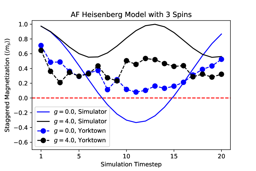
((a)) IBMQ Yorktown device

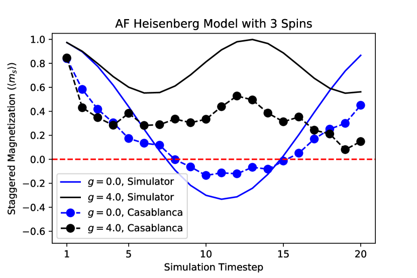
((b)) IBMQ Casablanca device

Figure 4. Results of simulation an AF model (eq. 1) for a system with three spins using the code snippet in Fig. 3 targeting the IBMQ’s Yorktown (a) and Casablanca (b) devices. Each data point is an average of five runs of 8192 measurement shots each. The circuits are compiled and optimized using the QCOR compiler before submitting for execution. The Trotter time-step ($dt$) is 0.05.

The simulation results from real quantum hardware for $g$ values of 0.0 and 4.0 are shown in Fig. 4, where we can see the effects of gate-errors and qubit decoherence leading to a significant impairment of the measured staggered magnetization (circles) compared to the theoretical values (solid lines). In particular, Fig. 4 demonstrates how the quality of the quantum hardware can affect simulation performance. The Yorktown backend has considerably worse performance metrics than the Casablanca backend. Specifically, compared to the Casablanca backend, Yorktown has a slightly higher two-qubit gate-error rate, nearly double the read-out error rate, and substantially lower qubit decoherence times. While identical quantum circuits were run on the two machines, we see much better distinguishability between the results for the two values of $g$ in the results from Casablanca than those from Yorktown.

The staggered magnetization response to a quench for a simple three-qubit AF Heisenberg model in Fig. 4, albeit noisy, illustrates non-trivial dynamics beyond that of decoherence (decaying to zero). Improvements in circuit construction (Trotter decomposition) and optimization, noise mitigation, and, most importantly, hardware performance (gate fidelity and qubit coherence) are required to scale up this time-domain simulation workflow for large quantum systems.

3.2. Variational Quantum Eigensolver

As a second use case demonstration, we apply the Variational Quantum Eigensolver (VQE) algorithm to find the ground state energy of ${\rm H}_{2}$. The VQE is a quantum-classic hybrid algorithm used to find a Hamiltonian’s eigenvalues, where the quantum process side is represented by a parametrized quantum circuit whose parameters are updated by a classical optimization process(peruzzo_variational_2014, ). The algorithm updates the quantum circuit parameters $\theta$ to minimize the Hamiltonian’s expectation value $E_{\theta}$ until it converges.

from qcor import * # Hamiltonian for H2 H = -0.22278593024287607*Z(3) + … +  0.04532220205777769*X(0)*X(1)*Y(2)*Y(3) -  0.09886396978427353 # Defining the ansatz @qjit def ansatz(q : qreg, params : List[float]): X(q[0]) … Rz(q[1],params[0]) Rz(q[3],params[1]) … Rz(q[3],params[2]) … H(q[3]) Rx(q[0], 1.57079) # variational parameters n_params = 3 # Create the problem model problemModel = QuaSiMo.ModelFactory.createModel(ansatz, H, n_params) # Create the optimizer: spsa optimizer = createOptimizer(’nlopt’, ’algorithm’:’spsa’) # Create the VQE workflow workflow = QuaSiMo.getWorkflow(’vqe’, ’optimizer’: optimizer) # Execute result = workflow.execute(problemModel) # Get the result energy = result[’energy’]

Figure 5. Code snippet to learn the ground state energy of ${\rm H}_{2}$ by the VQE. For the sake of simplicity, we have omitted most of the terms in the Hamiltonian and ansatz.

The performance of the VQE algorithm, as any other quantum-classical variational algorithms (benedetti_generative_2019, ), depends in part on the selection of the classical optimizer and the circuit ansatz. The design scheme implemented in this work allows us to tune the VQE components to pursue better performance. We present a listing of the code expressing this implementation in Fig. 5, in which we define the different parameters of the VQE algorithm in a custom-tailored way. In the code snippet, @qjit is a directive to activate the QCOR just-in-time compiler, which compiles the kernel body into the intermediate representation, and QuaSiMo.getWorkflow is a utility function of the library to construct and initialize workflow objects of various types. In Fig. 6(a), we present simulations considering the Simultaneous Perturbation Stochastic Approximation (SPSA) for ansatz updating. There, we show the energy as a function of the quantum circuits used in the learning process with a budget of 200 function evaluations with 5000 shots (experimental repetitions) per evaluation by using the QCOR’s VQE module, QuaSiMo.getWorkflow(’vqe’), and by using the Qiskit class aqua.algorithms.VQE (Qiskit-Aqua, ). In both cases, we consider $(0.,0.,0.)$ as the initial set of parameters, therefore the energy values in the first iterations are similar, due to the SPSA hyperparameter’s calibration. As it is expected, since we are using the same optimizer in both quantum simulations, there is not a relevant difference between the learning paths. However, the execution time in QCOR is shorter. This feature is presented in Fig. 6(b), where we show the execution time rate between QCOR and Qiskit as a function of the classical optimization algorithm. To evaluate the typical execution time of each optimizer, we consider 51 runs of VQE towards the generation of $H_{2}$ quantum ground state.

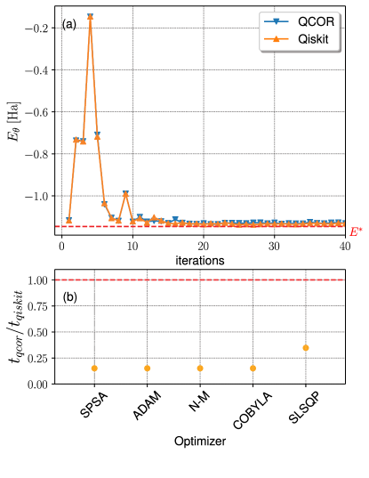
Figure 6. Energy ground state estimation for $H_{2}$ using VQE by using QCOR languange and Qiskit software. In panel (a), we present the VQE’s learning path using the stochastic algorithm SPSA to find a quantum state with minimal energy. This plot shows how the energy $E_{\theta}$ approaches the exact value $E^{*}=-1.1456295\ {\rm Ha}$ as the optimizer defines new quantum circuits, following the variational principle. In addition, panel (b), presents an execution time ratio between QCOR’s VQE module and Qiskit’s VQE module. The execution times ratio is below 1 (red dotted line) for different classical optimizers. The dots represent the 50th percentile of the execution time ratio from 51 independent runs of VQE. Optimizer labels correspond to Simultaneous Perturbation Stochastic Approximation (SPSA), ADAptive Moment estimation (ADAM), Nelder-Mead, also known as downhill simplex algorithm (N-M), Constraint Optimization By Linear Approximation (COBYLA), and the Sequential Least SQuares Programming (SLSQP).

3.2.1. Symmetry reduction

The presence of symmetries, such as rotations, reflections, number of particles, etc., in the Hamiltonian model allows us to map the model to a model with fewer qubits (Bravyi2017, ). In $H_{2}$, we apply the QCOR’s function operatorTransform(’qubit-tapering’, H) to reduce the four-qubit Hamiltonian, see Fig. 5, to a one-qubit Hamiltonian model. We present this implementation in Fig. 7, in which we transform the Hamiltonian introduced in Fig. 5 into a one-qubit model, and we redefine the anzats. In the output section of Fig. 7, we present the one-qubit model and the VQE’s output that converge to a similar value of the four-qubit model.

# Now we taper Hamiltonian H2 H_tapered = operatorTransform(’qubit-tapering’, H) # For the new Hamiltonian # we must define an one qubit ansatz @qjit def ansatz(q : qreg, phi : float, theta : float): Rx(q[0], phi) Ry(q[0], theta)

$Output:$ Reduced Hamiltonian: $(-0.328717,0)+(0.181289,0)X0+(-0.787967,0)Z0$ with energy = -1.13727017466

Figure 7. Symmetry reduction of the Hamiltonian model. In this snippet, we transform the Hamiltonian model used in 6 to a one-qubit model following symmetry arguments. This feature is implemented in the function operatorTransform(’qubit-tapering’, H).

3.2.2. Fermion-qubit map

from qcor import * @qjit def ansatz(q : qreg, x : List[float]): X(q[0]) with decompose(q, kak) as u: from scipy.sparse.linalg import expm from openfermion.ops import QubitOperator from openfermion.transforms import  get_sparse_operator qop = QubitOperator(’X0 Y1’)  - QubitOperator(’Y0 X1’) qubit_sparse = get_sparse_operator(qop) u = expm(0.5j * x[0] * qubit_sparse).todense() # Define the Hamiltonain H = -2.1433 * X(0) * X(1) - 2.1433 *  Y(0) * Y(1) + .21829 * Z(0) -  6.125 * Z(1) + 5.907 num_params = 1 # Create the VQE problem model problemModel = QuaSiMo.ModelFactory.createModel(ansatz, H, num_params) # Create the NLOpt derivative free optimizer optimizer = createOptimizer(’nlopt’) # Create the VQE workflow workflow = QuaSiMo.getWorkflow(’vqe’, ’optimizer’: optimizer) # Execute the workflow # to determine the ground-state energy result = workflow.execute(problemModel) energy = result[’energy’]

Figure 8. Here we depict how to use OpenFermion operators to construct the state-preparation kernel (ansatz) for the VQE workflow. We use SciPy (2020SciPy-NMeth, ) and OpenFermion (McClean2019OpenFermion, ) to construct the exponential of $(X_{0}Y_{1}-Y_{0}X_{1})$ operator as a matrix. The matrix will be decomposed into quantum gates by the QCOR compiler.

An important feature included in the QCOR compiler is the fermion-to-qubit mapping that facilitates the quantum state searching in VQE. In Fig. 8, we present an example of how to use OpenFermion operators (McClean2019OpenFermion, ) in the VQE workflow. In that implementation, we define the ansatz by using Scipy and OpenFermion, the QCOR compiler decomposes the ansatz into quantum gates; we follow the same structure presented in Fig. 5 for the VQE workflow.

3.3. Quantum Approximate Optimization Algorithm

To further demonstrate the utility of QCOR we present an implementation of the quantum approximate optimization algorithm (QAOA) (farhi2014quantum, ). QAOA translates a classical cost function into a quantum operator $H_{C}$ then uses a variational quantum-classical optimization loop to find quantum states that minimize the expectation value $\langle H_{C}\rangle$. The optimized quantum states are then prepared and measured to obtain bitstrings that correspond to classical solutions to the optimization problem.

Figure 9 shows example python code that uses QCOR simulations to find optimized quantum states with QAOA. Opening lines define the number of qubits $n$ and construct the problem Hamiltonian $H_{C}$ for MaxCut on a star graph $S_{n}$. The Hamiltonian is then used to create the QuaSiMo model and workflow to simulate $p$-step QAOA and return the expectation $\langle H_{C}\rangle$, similar to the previous VQE example of Fig. 5.

Figure 10 shows optimized energies $\langle H_{C}\rangle$ computed in QCOR for star graphs with numbers of qubits $n=2,...,9$ at various QAOA depth parameters $p$. Each time the program is run it begins with random initial parameters to be optimized, so we used several random starts for some of the graphs, keeping the smallest result as the $\langle H_{C}\rangle$ shown in the figure. The QCOR results are in perfect agreement with the optimized standards (lotshaw2021dataset, ) of Lotshaw et al.  (lotshaw2021empirical, ). The results have interesting features, for example when $n$ is odd perfect ground state energies $\langle H_{C}\rangle=E_{0}$ are obtained at $p=2$, while when $n$ is even the results need $p=3$ to approach close to $E_{0}$. The simplicity of the QCOR code and simulations make this an attractive route to studying interesting features like these in future research on QAOA.

from qcor import * # QAOA for unweighted MaxCut # Define a star graph Hamiltonian n_qubits = 8 H = 0 for n in range(1,n_qubits): H += -0.5*(1-Z(0)*Z(n)) # create QuaSiMo model problemModel = QuaSiMo.ModelFactory.createModel(H) # Create the NLOpt derivative-free optimizer optimizer = createOptimizer(’nlopt’) # QAOA steps p p = 3 # Quasimo workflow workflow = QuaSiMo.getWorkflow(’qaoa’, ’optimizer’: optimizer, ’steps’: p) # Execute the workflow # to determine the energy expectation value result = workflow.execute(problemModel) energy = result[’energy’]

Figure 9. Code to find the expectation value of the cost Hamiltonian with QAOA, for a star-graph instance of the unweighted MaxCut problem.

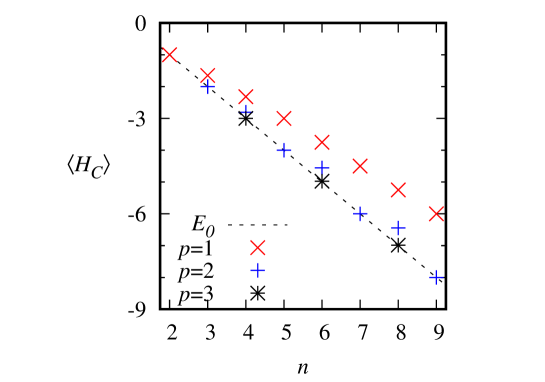
Figure 10. Optimized expectation values of the cost Hamiltonian $H_{C}$ for star-graph instances of unweighted MaxCut with QAOA.

3.4. Quantum Imaginary Time Evolution Algorithm

To compute the ground-state energy of an arbitrary Hamiltonian, in addition to VQE as we have demonstrated in 3.2, there is another algorithm, so-called Quantum Imaginary Time Evolution (QITE) (motta2019determining, ; Yeter_Aydeniz_2021, ), which does not require the use of an ansatz nor an optimizer. In QITE, we evolve the state through imaginary time $it\equiv\beta$ by applying the time-evolution operator $U=e^{-\beta H}$, which minimizes the system energy exponentially. To do so, for each imaginary time-step $\Delta\beta$, we approximate the imaginary time evolution based on the results of the previous steps.

As shown in Fig. 1, the QITE workflow is integrated into the QuaSiMo library. In this example, we demonstrate the use of QITE to find the ground state energy of a three-qubit transverse field Ising model (TFIM),

(3) $$H=J_{z}\sum_{i=1}^{N-1}\sigma_{i}^{z}\sigma_{i+1}^{z}+h_{x}\sum_{i=1}^{N}\sigma_{i}^{x}$$

where $J_{z}=h_{x}=-1.0$ and $N=3$ is the number of spins (qubits).

Fig. 11 is the code snippet to set up the QuaSiMo problem description and workflow for this problem.

⬇

// Initial state preparation

__qpu__ void state_prep(qreg q) {

// e.g., |100>

X(q[0]);

}

\par// Create the Hamiltonian: 3-qubit TFIM

auto observable = -(Z(0) * Z(1) + Z(1) * Z(2) +

X(0) + X(1) + X(2));

// Construct the problem model

auto problemModel =

ModelFactory::createModel(state_prep,

&observable);

\par// Create the qsearch IRTransformation

auto qsearch_optimizer =

createTransformation("qsearch");

// QITE workflow: 20 steps with dbeta = 0.45

// Also, use qsearch to optimize

// the propagating circuit.

auto workflow =

getWorkflow("qite",

{{"steps", 20},

{"step-size", 0.45},

{"circuit-optimizer",

qsearch_optimizer}});

// Execute

auto result = workflow->execute(problemModel);

Figure 11. Code snippet (in C++) to find the ground-state energy of a three-qubit TFIM Hamiltonian using the QITE workflow. In this example, we run the QITE algorithm for a total imaginary time $\beta$ of 9.0 ($d\beta=0.45$, 20 steps). Additionally, we use the QSearch algorithm from BQSKit to optimize QITE circuits during workflow execution. The state_prep kernel is used to initialize the qubits into the desired initial state, e.g., $|100\rangle$ in this particular case.

The problem model is captured by a single Hamiltonian operator constructed by direct Pauli operator algebra. We also want to note that the Pauli operator algebra of QuaSiMo allows for hierarchical construction of the Hamiltonian, e.g., via for loops, suitable for generic Hamiltonians similar to the one described in eq. (3).

For QITE workflow configurations, we set step-size to 0.45 and steps to 20, for a total imaginary time of $\beta=9.0$ ($\hbar=1$). The system begins in different initial states by using a state-preparation circuit, as shown in Fig. 11. Similar to the Python API, users can also use the utility function getWorkflow to retrieve an instance of the QITE workflow from the QCOR service registry with the name key "qite" as shown in Fig. 11.

The main drawback of QITE algorithm is that the propagating circuit size increases during the imaginary time-stepping procedure. To alleviate this constraint, especially for execution on NISQ hardware, QuaSiMo’s QITE workflow implementation support custom, externally-provided circuit optimizers that will be invoked during the algorithm execution to minimize the circuit depth. In this demonstration, we take advantage of the QSearch (qsearch, ) optimizer from BQSKit library, which is capable of synthesizing constant-depth circuits for a variety of common use cases including the TFIM model in (3). For instance, in this example, the final QITE circuit (step = 20) has approximately 8,000 gates (3,000 CNOT gates), which is clearly beyond the capability of current NISQ devices. Thanks to QSearch, we can always re-synthesize a constant depth circuit with only 14 CNOT gates (87 gates in total) for any of the time steps, which is the theoretical lower bound (PhysRevA.69.062321, ), $\frac{1}{4}(4^{n}-3n-1)=13.5$, for CNOT gate count in three-qubit circuits.

Figure 12. QITE results for 3-qubit TFIM with different initial states, step size = 0.45. The red dashed line represents the true ground-state energy of -3.49396.

The results of the QITE workflow execution are shown in Fig. 12, where we can see the energy value exponentially decays to the analytically computed ground state energy of -3.49396 for all initial states.

4. Conclusions

We have presented and demonstrated a programming workflow for applications of quantum simulation that promotes common, reusable methods and data structures for scientific applications.

We note that while the framework presented here is readily applicable to use cases in the NISQ era - with the QuantumSimulationWorkflow in particular being extendable to NISQ simulation algorithms such as VQE - the workflow is also extendable to universal algorithms. Code portability is ensured through intermediate representation that is then implemented for each backend according to specific APIs, which are accessible in the QuaSiMo library. This enables rapid porting of a simulation algorithm to multiple machines (write once, run everywhere paradigm). This is an ideal environment in which to construct both benchmarks and validation protocols, along with short depth quantum simulations that can quickly be run on multiple processors and directly compared.

While we maintain a focus on rapid prototyping of quantum simulation on today’s NISQ devices, we note that the nature of the intermediate representation and the modular backend structure enable targeting fault tolerant devices as well. A fault tolerant (FT) architecture may be represented as an additional backend with encoding transpiler preprocessing. While this configuration is ideal for QuaSiMo’s unencoded qubit targets, we also note that the parent language QCOR, is capable of expressing fully quantum-error-correction-encoded algorithms as well. Therefore, we expect the framework to be extendable and to find use in workflows involving universal or FT applications in the future.

References

- (1) Aspuru.Guzik, A., Dutoi, A.D., Love, P.J., Head.Gordon, M.: ‘Simulated quantum computation of molecular energies’, Science, 2005, 309, (5741), pp. 1704–1707
- (2) Whitfield, J.D., Biamonte, J., Aspuru.Guzik, A.: ‘Simulation of electronic structure hamiltonians using quantum computers’, Molecular Physics, 2011, 109, (5), pp. 735–750
- (3) Cao, Y., Romero, J., Olson, J.P., Degroote, M., Johnson, P.D., Kieferová, M., et al.: ‘Quantum chemistry in the age of quantum computing’, Chemical reviews, 2019, 119, (19), pp. 10856–10915
- (4) McArdle, S., Endo, S., Aspuru.Guzik, A., Benjamin, S.C., Yuan, X.: ‘Quantum computational chemistry’, Reviews of Modern Physics, 2020, 92, (1), pp. 015003
- (5) Yeter.Aydeniz, K., Siopsis, G., Pooser, R.C.: ‘Scattering in the ising model using quantum lanczos algorithm’, arXiv preprint arXiv:200808763, 2020,
- (6) O’Malley, P.J., Babbush, R., Kivlichan, I.D., Romero, J., McClean, J.R., Barends, R., et al.: ‘Scalable quantum simulation of molecular energies’, Physical Review X, 2016, 6, (3), pp. 031007
- (7) Lidar, D.A., Wang, H.: ‘Calculating the thermal rate constant with exponential speedup on a quantum computer’, Physical Review E, 1999, 59, (2), pp. 2429
- (8) Bassman, L., Liu, K., Krishnamoorthy, A., Linker, T., Geng, Y., Shebib, D., et al.: ‘Towards simulation of the dynamics of materials on quantum computers’, Physical Review B, 2020, 101, (18), pp. 184305
- (9) Kosugi, T., Matsushita, Y.i.: ‘Linear-response functions of molecules on a quantum computer: Charge and spin responses and optical absorption’, Physical Review Research, 2020, 2, (3), pp. 033043
- (10) Lysne, N.K., Kuper, K.W., Poggi, P.M., Deutsch, I.H., Jessen, P.S.: ‘Small, highly accurate quantum processor for intermediate-depth quantum simulations’, Phys Rev Lett, 2020, 124, pp. 230501. Available from: https://link.aps.org/doi/10.1103/PhysRevLett.124.230501
- (11) Cirstoiu, C., Holmes, Z., Iosue, J., Cincio, L., Coles, P.J., Sornborger, A.: ‘Variational fast forwarding for quantum simulation beyond the coherence time’, npj Quantum Information, 2020, 6, (1), pp. 1–10
- (12) Quantum, G.A., et al.: ‘Hartree-fock on a superconducting qubit quantum computer’, Science, 2020, 369, (6507), pp. 1084–1089
- (13) McClean, J.R., Romero, J., Babbush, R., Aspuru.Guzik, A.: ‘The theory of variational hybrid quantum-classical algorithms’, New Journal of Physics, 2016, 18, (2), pp. 023023
- (14) Romero, J., Babbush, R., McClean, J.R., Hempel, C., Love, P.J., Aspuru.Guzik, A.: ‘Strategies for quantum computing molecular energies using the unitary coupled cluster ansatz’, Quantum Science and Technology, 2018, 4, (1), pp. 014008
- (15) Grimsley, H.R., Economou, S.E., Barnes, E., Mayhall, N.J.: ‘An adaptive variational algorithm for exact molecular simulations on a quantum computer’, Nature Communications, 2019, 10, (1), pp. 1–9
- (16) Tang, H.L., Barnes, E., Grimsley, H.R., Mayhall, N.J., Economou, S.E.: ‘qubit-adapt-vqe: An adaptive algorithm for constructing hardware-efficient ansatze on a quantum processor’, arXiv preprint arXiv:191110205, 2019,
- (17) Farhi, E., Goldstone, J., Gutmann, S.: ‘A quantum approximate optimization algorithm’, arXiv:14114028, 2014,
- (18) Motta, M., Sun, C., Tan, A.T., O’Rourke, M.J., Ye, E., Minnich, A.J., et al.: ‘Determining eigenstates and thermal states on a quantum computer using quantum imaginary time evolution’, Nature Physics, 2019, pp. 1–6
- (19) Qiskit. ‘Qiskit aqua’. (Qiskit, 2021. Available from: https://github.com/Qiskit/qiskit-aqua
- (20) Qiskit. ‘Qiskit terra’. (Qiskit, 2021. Available from: https://github.com/Qiskit/qiskit-terra
- (21) Kottmann, J.S., Alperin.Lea, S., Tamayo.Mendoza, T., Cervera.Lierta, A., Lavigne, C., Yen, T.C., et al.: ‘Tequila: A platform for rapid development of quantum algorithms’, arXiv preprint arXiv:201103057, 2020,
- (22) Zapata. ‘Orquestra’. (Zapata, 2021. Available from: https://www.zapatacomputing.com/orquestra
- (23) Kandala, A., Mezzacapo, A., Temme, K., Takita, M., Brink, M., Chow, J.M., et al.: ‘Hardware-efficient variational quantum eigensolver for small molecules and quantum magnets’, Nature, 2017, 549, (7671), pp. 242
- (24) Hempel, C., Maier, C., Romero, J., McClean, J., Monz, T., Shen, H., et al.: ‘Quantum chemistry calculations on a trapped-ion quantum simulator’, Physical Review X, 2018, 8, (3), pp. 031022
- (25) McCaskey, A.J., Parks, Z.P., Jakowski, J., Moore, S.V., Morris, T.D., Humble, T.S., et al.: ‘Quantum chemistry as a benchmark for near-term quantum computers’, npj Quantum Information, 2019, 5, (1), pp. 1–8
- (26) Yeter.Aydeniz, K., Pooser, R.C., Siopsis, G.: ‘Practical quantum computation of chemical and nuclear energy levels using quantum imaginary time evolution and lanczos algorithms’, npj Quantum Information, 2020, 6, (1), pp. 1–8
- (27) Qiskit. ‘Introducing qiskit nature’. (Qiskit, 2021. Available from: https://medium.com/qiskit/introducing-qiskit-nature-cb9e588bb004
- (28) Nguyen, T., Santana, A., Kharazi, T., Claudino, D., Finkel, H., McCaskey, A.: ‘Extending c++ for heterogeneous quantum-classical computing’, arXiv preprint arXiv:201003935, 2020,
- (29) Marples, D., Kriens, P.: ‘The Open Services Gateway Initiative: An introductory overview’, Communications Magazine, IEEE, 2002, 39, (12), pp. 110–114
- (30) ‘Source code repository’. (GitLab, 2020. https://code.ornl.gov/elwasif/qsa-workflow
- (31) Britt, K.A., Humble, T.S.: ‘High-performance computing with quantum processing units’, ACM Journal on Emerging Technologies in Computing Systems (JETC), 2017, 13, (3), pp. 1–13
- (32) McCaskey, A.J., Dumitrescu, E.F., Liakh, D., Chen, M., Feng, W., Humble, T.S.: ‘A language and hardware independent approach to quantum–classical computing’, SoftwareX, 2018, 7, pp. 245 – 254. Available from: http://www.sciencedirect.com/science/article/pii/S2352711018300700
- (33) Marples, D., Kriens, P.: ‘The open services gateway initiative: An introductory overview’, IEEE Communications magazine, 2001, 39, (12), pp. 110–114
- (34) Mintz, T.M., McCaskey, A.J., Dumitrescu, E.F., Moore, S.V., Powers, S., Lougovski, P.: ‘Qcor: A language extension specification for the heterogeneous quantum-classical model of computation’, ACM Journal on Emerging Technologies in Computing Systems (JETC), 2020, 16, (2), pp. 1–17
- (35) Trotter, H.F.: ‘On the product of semi-groups of operators’, Proceedings of the American Mathematical Society, 1959, 10, (4), pp. 545–551
- (36) Suzuki, M.: ‘Generalized trotter’s formula and systematic approximants of exponential operators and inner derivations with applications to many-body problems’, Communications in Mathematical Physics, 1976, 51, (2), pp. 183–190
- (37) Barkoutsos, P.K., Gonthier, J.F., Sokolov, I., Moll, N., Salis, G., Fuhrer, A., et al.: ‘Quantum algorithms for electronic structure calculations: Particle-hole hamiltonian and optimized wave-function expansions’, Physical Review A, 2018, 98, (2), pp. 022322
- (38) O’Brien, T.E., Polla, S., Rubin, N.C., Huggins, W.J., McArdle, S., Boixo, S., et al.: ‘Error mitigation via verified phase estimation’, arXiv preprint arXiv:201002538, 2020,
- (39) ‘Qcor - c++ compiler for heterogeneous quantum-classical computing built on clang and xacc’. (GitHub, 2020. https://github.com/ORNL-QCI/qcor
- (40) Barmettler, P., Punk, M., Gritsev, V., Demler, E., Altman, E.: ‘Quantum quenches in the anisotropic spin-heisenberg chain: different approaches to many-body dynamics far from equilibrium’, New Journal of Physics, 2010, 12, (5), pp. 055017
- (41) Preskill, J.: ‘Quantum computing in the nisq era and beyond’, Quantum, 2018, 2, pp. 79
- (42) Wiebe, N., Berry, D.W., Høyer, P., Sanders, B.C.: ‘Simulating quantum dynamics on a quantum computer’, Journal of Physics A: Mathematical and Theoretical, 2011, 44, (44), pp. 445308
- (43) Peruzzo, A., McClean, J., Shadbolt, P., Yung, M.H., Zhou, X.Q., Love, P.J., et al.: ‘A variational eigenvalue solver on a photonic quantum processor’, Nature Communications, 2014, 5, (1), pp. 4213. Available from: https://doi.org/10.1038/ncomms5213
- (44) Benedetti, M., Garcia.Pintos, D., Perdomo, O., Leyton.Ortega, V., Nam, Y., Perdomo.Ortiz, A.: ‘A generative modeling approach for benchmarking and training shallow quantum circuits’, npj Quantum Information, 2019, 5, (1), pp. 45. Available from: https://doi.org/10.1038/s41534-019-0157-8
- (45) Bravyi, S., Gambetta, J.M., Mezzacapo, A., Temme, K.: ‘Tappering off qubits to simulate fermionic hamiltonian’, arXiv preprint arXiv:170108213, 2017,
- (46) Virtanen, P., Gommers, R., Oliphant, T.E., Haberland, M., Reddy, T., Cournapeau, D., et al.: ‘SciPy 1.0: Fundamental Algorithms for Scientific Computing in Python’, Nature Methods, 2020, 17, pp. 261–272
- (47) McClean, J.R., Sung, K.J., Kivlichan, I.D., Cao, Y., Dai, C., Fried, E.S., et al.: ‘Openfermion: The electronic structure package for quantum computers’, , 2019,
- (48) Lotshaw, P.C., Humble, T.S.. ‘QAOA dataset’. (, 2021. Available from: https://code.ornl.gov/qci/qaoa-dataset-version1
- (49) Lotshaw, P.C., Humble, T.S., Herrman, R., Ostrowski, J., Siopsis, G.: ‘Empirical performance bounds for quantum approximate optimization’, arXiv:2102:06813, 2021,
- (50) Yeter.Aydeniz, K., Siopsis, G., Pooser, R.C.: ‘Scattering in the ising model with the quantum lanczos algorithm’, New Journal of Physics, 2021, 23, (4), pp. 043033. Available from: https://doi.org/10.1088/1367-2630/abe63d
- (51) Davis, M.G., Smith, E., Tudor, A., Sen, K., Siddiqi, I., Iancu, C. ‘Towards optimal topology aware quantum circuit synthesis’. In: 2020 IEEE International Conference on Quantum Computing and Engineering (QCE). (, 2020. pp. 223–234
- (52) Shende, V.V., Markov, I.L., Bullock, S.S.: ‘Minimal universal two-qubit controlled-not-based circuits’, Phys Rev A, 2004, 69, pp. 062321. Available from: https://link.aps.org/doi/10.1103/PhysRevA.69.062321