Anomaly detection with Convolutional Graph Neural Networks
Abstract
We devise an autoencoder based strategy to facilitate anomaly detection for boosted jets, employing Graph Neural Networks (GNNs) to do so. To overcome known limitations of GNN autoencoders, we design a symmetric decoder capable of simultaneously reconstructing edge features and node features. Focusing on latent space based discriminators, we find that such setups provide a promising avenue to isolate new physics and competing SM signatures from sensitivity-limiting QCD jet contributions. We demonstrate the flexibility and broad applicability of this approach using examples of bosons, top quarks, and exotic hadronically-decaying exotic scalar bosons.
1 Introduction
The search for new physics beyond the SM (BSM), albeit unsuccessful so far at high energy colliders such as the Large Hadron Collider (LHC), remains a key pillar of the particle physics phenomenology programme. The mounting pressure of exclusion constraints for well-motivated BSM scenarios reported by the ATLAS and CMS experiments has shifted theoretical efforts more towards model-independent approaches for new physics discoveries. This is most prominently reflected in the recent resurgence of effective field theory interpretations of collider data (see e.g. Ref. Brivio:2017vri for a recent review).
One method of searching for the presence of new BSM interactions is attempting to detect anomalies in otherwise well-understood and abundant collider data Collins:2021nxn ; CMS:2020zjg ; Aaboud:2018ufy ; Collins:2018epr ; Blance:2019ibf ; Hajer:2018kqm ; DeSimone:2018efk ; Nachman:2020lpy ; Nachman:2020ccu . Hard jets produced primarily via QCD-mediated interactions at hadron colliders are a well-known laboratory for such strategies and their phenomenology has seen considerable development over the past decade Marzani:2019hun . QCD jets are produced with large rates at the LHC even when they are extremely hard, and therefore are the typical backgrounds that any search for new physics in hadronic final states needs to overcome. Turning this argument around, we can classify jets, possibly using motivated first-principle approaches Soper:2011cr ; Soper:2014rya , and isolate more interesting generic BSM-type signatures by vetoing a “typical” QCD jet. Following this line of thought, anomaly-detection has become a primary application of unsupervised machine learning. This typically involves so-called autoencoders, which are artificial neural networks specifically tailored to reproduce the most common properties of a training data set via a reduction of the dimensionality of the input’s features. When a jet behaves less like a common QCD jet (e.g. in case of a particular hadronic BSM decay) such a network should perform poorly, i.e. the loss that parametrises the networks ability to reproduce the QCD signature can be used as a BSM-discriminating observable.
The evolution of a typical QCD event from high to low energies is well understood over a vast range of energy scales, as demonstrated by the successful application of QCD shower Monte Carlo programmes to the modelling of collider data (see e.g. Aad:2014qxa ). This evolution also motivates the application of Graph Neural Networks (GNNs) zhou2018graph ; 9046288 to QCD phenomenology as recently done in Refs. Dreyer:2020brq , and also to exploiting the Lund-plane representation of splittings Andersson:1988gp ; Lifson:2020gua . GNNs have also been studied in various scenarios Mikuni:2020wpr ; Knapp:2020dde ; Mikuni:2020qds ; Dezoort:2021kfk ; Abdughani:2018wrw at the LHC. Moreover, they have also shown promising performances for use in real-time triggers Iiyama:2020wap . In this work we consider a GNN-based autoencoder for anomaly detection in boosted QCD jets data. Convolutional autoencoders have been proposed and studied in Farina:2018fyg ; Heimel:2018mkt ; Roy:2019jae ; Khosa:2020qrz ; Finke:2021sdf ; Cheng:2020dal for distinguishing QCD jets from non-QCD jets using “jet-images” Cogan:2014oua ; deOliveira:2015xxd as the input space. However, convolutions on these images are expensive due to their extreme sparsity. Moreover, CNNs, in principle, are limited to the Euclidean domain. GNNs mitigate these two inadequacies, so studying their performance as anomaly finders is motivated. Supervised jet classification with GNNs has been studied in Ref. Ju:2020tbo ; Qu:2019gqs ; Dreyer:2020brq , while unsupervised clustering of event-graphs with photonic quantum computers have been explored in Ref. Blance:2021gcs .A study of particle graph autoencoders for anomaly detection has been carried out in the LHC Olympics community challenge kasieczka2021lhc . A typical obstacle of GNN-based autoencoders is achieving an appropriate reflection of all network features on the decoding side. Existing graph-autoencoders in the literature kipf2016variational ; tran2018learning ; salha2020simple ; pan2018adversarially ; park2019symmetric are designed mostly for node-classification or link prediction, while we desire a network capable of classifying graphs. Moreover, jets provide us with multidimensional edge information, along with node features; classifying the entire graph thereby exploits the full kinematic information of the event. To solve this known difficulty of graph-autoencoders, we design a decoder network capable of simultaneously reconstructing multidimensional edge, and node features with the help of Inner Product Layers.
2 Elements of the Simulation
For our proof-of-principle analysis111Throughout this work, we will focus on 13 TeV LHC collisions., we generate events using MadGraph5 Alwall:2014hca at leading order (LO), followed by Pythia8 Sjostrand:2006za for showering and hadronization. The hadronic final states are then clustered into jets using the anti- algorithm Cacciari:2008gp with parameter using FastJet Cacciari:2011ma . Along with a requirement that the rapidity of jets is , the minimum transverse momentum of a jet is required to be for this “fat jet” cluster. Only the leading jet from each multi-jet event is used as an input to the graph network and we do not include detector effects to our analysis. The sample used for training of the autoencoder (for details see below) is a QCD multi-jet background sample, consisting of 200k generated events.
To test the autoencoder’s anomaly detection performance we use three different signal samples, each consisting of 100k events generated with MadGraph5, using the same procedure described above. These samples consist of
-
(i)
boosted hadronically-decaying bosons as a benchmark for two-prong jet structure,
-
(ii)
boosted hadronically-decaying top quarks, as a benchmark for a three-prong structure, and
-
(iii)
a boosted scalar decaying as to give a four-prong structure. The interaction is based on a simplified Lagrangian
(1) where and are dimensionless constants and is the Higgs field’s vacuum expectation value (vev). We choose for demonstration purposes, but note that our results are not too sensitive to the mass scale.
To map out an infrared safe input to the graph network, we first use the anti- jet algorithm to re-cluster the fat jet constituents into microjets222As shown in Ref. ATLAS:2014twa , such objects are under good experimental control. with a finer resolution of and minimum . We consider fat jets with at least three microjets for our neural network analysis.
Identifying each microjet as a node in the network, we construct a graph associated with each jet as follows:
-
•
Node feature vectors: We associate five microjet observables as the node’s feature vector . These are and . Here, is the transverse momentum of the microjet, and are differences in pseudorapidity, azimuthal angle, and angular distance between the microjet and the jet axis respectively. is the mass of the microjet divided by 100 GeV, which, along with the log on , reduces the disparity in the range with the other three angular variables.
-
•
Edge feature vectors: After the nodes are defined, we define the graph as the complete graph with all possible edge connections. For each edge, we construct an associated edge-feature vector of three dimensions. Its components are the two distance parameters between the nodes as defined below, and one invariant mass parameter: . The metric is given by
where for Cambridge-Aachen (CA) jets, for jets and is radius parameter for the fat jet. The CA measure provides information about the geometric distance between two microjets, whereas the measure is motivated from QCD splittings Catani:1991hj ; Ellis:1993tq . is the invariant mass of the two microjets. These three variables capture the essential physics between two nodes.
-
•
Adjacency Matrix: We also construct the adjacency matrix for each edge feature to facilitate their reconstruction at the decoder side. It is defined as
where is the vectorial index. Thus, for a jet-graph of nodes, we have three matrices. The network outputs the edge-features in this representation, and hence the edge-loss is defined as a function of these adjacency matrices.
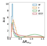
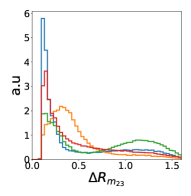
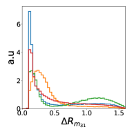
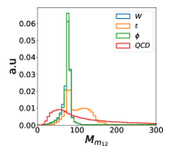
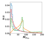
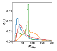
The distribution of and for the 3-leading microjets of each jet are shown in Figs. 1 and 2. The construction of the graphs and the network analysis are performed using the Deep Graph Library wang2020deep with the PyTorch paszke2019pytorch backend.

3 Graph Neural Networks
In this section, we describe the various components of our neural network analysis. We briefly detail the conceptual structure of GNNs before moving on to describe the ones we utilise in our analysis, along with the explicit form of the autoencoder’s loss function. The network architecture and the process of training are described thereafter.
Graph Neural Networks are models that can extract features from graph-structured data. They generalise the inbuilt inductive biases in Convolutional Neural Networks (CNNs) like local connectivity and shared weights to variable length and possibly non-Euclidean data 726791 . For supervised learning applications, this was formalised as Message Passing Neural Networks (MPNNs) in Ref. gilmer2017neural . We sketch the general paradigm and then describe in greater detail the two specific forms that are used in our work in the succeeding paragraphs. In the following, is the node’s features at the timestep (analogous to a layer in the usual ANNs). denotes the features of the edge connecting the nodes and , and is the set of nodes connected to the node . For the input layer, we take , and . MPNNs consist of a message passing phase and a graph readout layer. In the first phase, a message-passing function is defined for two nodes and
| (2) |
which calculates the message for the edge connecting the nodes. The message function is usually a multilayer-perceptron (MLP) shared between all the edges, hence the term graph convolutions. For each timestep (or layer), the messages between all connected nodes are calculated, after which the features of each node are updated according to an aggregation function
| (3) |
which is a function of the node feature and all incoming333The message passing function need not be symmetric in and . messages. The updated features , are used for the next timestep to perform another message passing and aggregation step. At the output of the final message-passing timestep, a graph readout layer performs a permutation-invariant444A permutation invariant function makes the output invariant to graph isomorphisms. operation (for instance, max, sum, or mean) on the node features to give fixed-length vectors, regardless of the number of nodes. In supervised learning, this vector can be the final output which can be used either to minimise the loss function or fed into an MLP. However, in a graph-autoencoder, graph-level readouts are not applied to preserve the graph structure until the final output. Graph-autoencoders are typically designed for classifying nodes or edges, focusing on learning local features of a huge graph. However, as our goal is to classify small graphs, the network needs to learn global graph structures and local features. To overcome this, we design an edge-reconstruction network within the decoder, making our network capable of learning graph structures by reconstructing the graph in its entirety. The complete structure of our network is shown in Fig. 3, where the black boxes encase the encoder and the decoder. The edge-reconstruction network is shown bounded by the blue box. These are described in greater detail in the following passages.
3.1 Autoencoder
Autoencoders are neural networks that map an input space to a bottleneck dimension (the latent dimension) and then back again to a space identical to the input. We use the graph-convolutions proposed in Ref. gilmer2017neural to incorporate the multi-dimensional edge information along with the input node features. Our network, therefore, learns the physics information that is encoded into our 3-dimensional edge feature. The timesteps until we reach the latent space employ edge-convolution wang2019dynamic , which has proved excellent performance in supervised learning scenarios Qu:2019gqs ; Dreyer:2020brq . We refer to these two layers as NNConv, and EdgeConv respectively, according to the python class name implemented in the Deep Graph Library. The encoder block outputs a graph with the same edge connections as that of the input with updated latent features for each node. The decoder reconstructs the node and edge features from this latent node representation. As shown in Fig. 3, the decoder has a shared block of edge convolutions, after which the output feeds into four different blocks of edge convolutions: a single layer for the node reconstruction, and three edge reconstruction blocks. These three blocks are identical in structure and reconstruct each edge feature independently from the propagated information from the shared block. We use an Inner Product Layer kipf2016variational to reconstruct the edge information in the form of three adjacency matrices. These three components and the composition of the loss function are explained in the subsequent paragraphs.
NNConv: The first layer takes the node and edge features as input and performs a weighted graph convolution by making use of an MLP, referred to as edge function . This takes the edge features as input and maps it to a dimension of , where is the input node’s dimensions (5 in the present case), and is the dimension of the updated node features. The message passing function performs a broadcasted element-wise multiplication of the form
| (4) |
where and are the indices of the matrix, and is formed by repeating , the input node features, times. The aggregation step takes the mean of over all neighbouring nodes , and then sums over the index of the matrix:
| (5) |
to give updated dimensional node features .
EdgeConv: The backbone of our architecture is the edge convolution operation wang2019dynamic . This involves two linear layers: and , with identical input and output dimensions, which determine the dimensions of original and updated node features respectively. The message passing function is defined as
| (6) |
while the aggregation step involves taking the maximum value
| (7) |
in each component of the incoming message vectors to give the updated node features .
Inner Product Layer: The edge-reconstruction network uses an Inner Product Layer to reconstruct the edge features from the node features of the final edge convolution output. The inner product makes the correspondence to the two-node indices for each edge. Since our graphs are undirected, the layer constructs a symmetric matrix, being the number of nodes in the graph. Its components are therefore
| (8) |
where and are node-feature vectors.
Loss Function: We use root-mean squared error (RMSE) for the node as well as the edge reconstruction losses. For the node feature this is
| (9) |
where is the node-feature index, is the node index, and are the reconstructed and input node features, respectively. We define the edge reconstruction loss as the sum of three individual RMSEs for each edge feature
| (10) |
where is the edge-feature index, and are node indices. and are the reconstructed and input adjacency matrices respectively. The total loss is the weighted sum of the individual losses,
| (11) |
We choose and , so that the combined node features get the same weight as each individual edge feature, which carry more relevant physics information. Note that the loss function is invariant to node permutations of the input graph since, mean is a permutation invariant function, and the architecture respects permutation invariance: any change in the node ordering changes the output of each layer(via the graph readout) in conjunction with the adjacency matrix. Our network however, does not reconstruct an arbitrarily permuted graph for a given input, which is not strictly necessary since we concentrate on the reconstruction error of a single graph and not of an equivalence class of graphs.
3.2 Network Architecture and training
Neural networks require a careful optimal choice of hyperparameters. As this is a proof-of-principle analysis, we do not perform an extensive hyperparameter scan. However, we scan over the latent dimension, which is critical for any autoencoder. For the first layer of the graph-encoder (NNConv), we use an MLP of hidden dimensions: 256, 128, 64, and 32 as the edge function to map the 3-dimensional edge features to a dimensional output. The hidden layers have ReLU activations, whereas the final layer has a sigmoid activation. The limited range of the sigmoid activation helps in giving the addition operation in aggregation (as defined in Eq. (5)) an interpretation of a weighted sum over messages in an additional dimension without the dynamics being entirely dominated by the outputs of the edge function. Each hidden layer has a dropout layer with fraction 0.2 of disconnected nodes between layers to avoid overfitting and achieve better generalisation. After the aggregation, we get a 128-dimensional output that feeds into a series of edge-convolution layers with linear layers as and . The output dimensions of the linear layers are 64 and 32 and outputs a 6 dimensional latent node encoding. This value is chosen after a scan over different latent dimensions which we elaborate on in the next section. The shared block of the decoder uses the encoder’s reversed dimensions: 32, 64, and 128. With the 128-dimensional vector as input, the node reconstruction layer performs an edge-convolution to give the reconstructed node vectors . Similarly, each edge reconstruction network has three successive edge convolutions of output dimensions 32, 16, and 8. We calculate the inner products on the 8-dimensional vector space to give the reconstructed adjacency matrices .
We train the network with the Adam optimiser kingma2014adam initialised with a 0.001 learning rate on mini-batches of 64 samples. The learning rate is decayed with a reduce-on-plateau condition with decay factor 0.5, and a patience of five epochs with an additional five epochs of cool-down. We use 85k jets to train the network. After each epoch, we calculate the loss of an independent validation dataset containing 28k QCD jets. We stop the training once the learning rate goes below . The epoch with minimum validation loss is used for further inference.
4 Results and Discussion
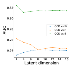
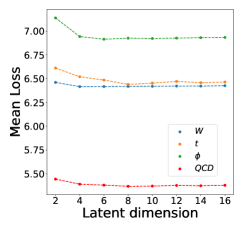
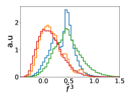
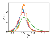
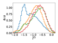
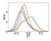
In order to test the performance of the graph-autoencoder for the different non-QCD signals described in Sec. 2, we evaluate the discrimination power of the total loss function as defined in Eq. (11). We use an independent testing data set of 28k for QCD jets and a similar number for the signal samples. We first scan the latent dimension from 2 to 12 in multiples of two, keeping all other hyperparameters fixed. The Area-Under-(the)Curve (AUC) between the signal acceptance and the background rejection for each latent dimension is shown in Fig. 4(a). In Fig. 4(b), we show the mean loss for each class as a function of the latent dimension. We can see that although the mean loss is relatively stable for QCD jets after 4-dimensions, the AUC of the different signal vs. QCD scenarios varies significantly. The variation is due to the unsupervised nature of the algorithm; the network has no information about the signal classes.
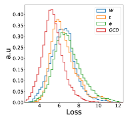
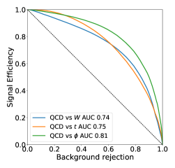
On the other hand, from the different nature of the AUC curves, we can understand the information passed for differing latent dimensions. The increasing AUCs for the classification hints that the network sees them as similar to QCD jets when the information passed in the bottleneck is smaller, but the features of a typical QCD jet are not fully modelled for low dimensions, thus making this discrimination not reliable. Increasing the bottleneck dimension makes the network learn QCD features, which then leads to robust anomaly detection for top quarks and bosons. The jets, which have the most noticeably different structure from QCD jets, reach a stable AUC much faster than tops and bosons. We infer that latent dimension of shows a stable performance for all three classes (in particular for QCD jets) and has reached the plateau in the mean loss. Since we cannot optimise the network to each class in anomaly detection, we fix six as the latent dimension parameter. The normalised distribution of the loss function for all classes is shown in Fig. 5(a). As the network is trained using QCD jets, the autoencoder reconstructs them with lower loss, while all signal classes have a relatively higher loss. By vetoing the QCD jets with lower losses, we tag (new physics) signal jets (anomalous class); the Receiver-Operator-Characteristic (ROC) curve between the signal acceptance and background rejection is shown in Fig. 5(b)555We compare the results obtained for our dataset with particle graph autoencoders used in Ref kasieczka2021lhc in Appendix A.. The performance increases as the prong structure becomes richer for the signal classes. We discuss the correlation of the loss with some important jet-level observables in Appendix B.
We also investigate the latent representation learned by the graph-autoencoder to explore compressed representations for QCD jets. Latent representations have also been investigated in similar, and indeed different, physical scenarios recently in Refs. Dillon_2020 ; bortolato2021bump ; dillon2021better . Even though we do not perform graph readouts during the training, the graph-autoencoder learns the graph structure via the edge reconstruction network. We use a graph readout that takes the mean in each dimension of the latent node features to obtain a fixed-dimensional latent graph representation. More precisely, we consider
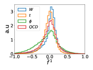
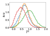
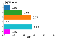
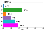
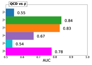
where is the vector-index, is the node index and is the set of all nodes of the graph. The normalised distribution of the four classes for each latent dimension is shown in Fig. 6, while the corresponding AUC for each signal vs. QCD discrimination is shown in Fig. 7. We find that performs best for top and jets, while gives the maximum AUC for jets. The AUC for top quarks and scalar from is 0.74 and 0.84 respectively. Thus, we find a significant improvement for from the value obtained with the loss function, which is also the case for the jets whose AUC is 0.78 from . The latent distributions are prone to training uncertainties since they do not have any regularising terms in the loss function.
More precisely, the shapes and location of these distributions will vary significantly for different training instances even when they give very similar distributions of the loss function. There are available remedies kingma2014autoencoding ; makhzani2015adversarial ; patrini2019sinkhorn for the training class, but controlling the signal distributions during unsupervised training is not possible by design. However, it may be possible to control them using physically motivated priors, which is beyond the scope of our present work. Nevertheless, once we have a single training instance, latent dimension-based anomaly finders can be used by trimming the encoder network after training to contain only these two outputs. Control samples can be used to quantify the latent space distributions and could therefore find applications in trigger optimisation.
5 Conclusions
In this work, we have introduced a graph neural network-based autoencoder for unsupervised anomaly detection in QCD boosted jet data. We design a novel edge-reconstruction network for the graph-decoder, which allows us to reconstruct multidimensional edge information. This gives the graph-autoencoder the capacity to classify entire graphs, unlike previously existing graph-autoencoders. We use NNConv to incorporate the multidimensional edge and node features as inputs to a graph-autoencoder while utilising edge convolutions to learn inductive latent space representations of QCD jets’ graph-structured data.
The anomaly finder based on the reconstruction loss shows good performance for the non-QCD scenarios that we consider. We further explore the possibility of exploiting latent space variables as discriminants for anomalous jets and find that latent variables can indeed lead to improved anomaly detection by accessing the compressed information of the QCD data. While GNNs are known to be good candidates for trigger-level implementations, we study latent dimension-based anomaly finders with graph-autoencoders. Using latent dimensions instead of the loss has the additional appeal of halving the number of layers, thus resulting in a shallower network. Studying the latent dimension representation of QCD jets therefore provides a compressed arena for new physics discovery by using these observables directly.
Acknowledgements
O.A. is supported by the UK Science and Technology Facilities Council (STFC) under grant ST/V506692/1. A.B. and C.E. are supported by the STFC under grant ST/T000945/1. C.E is also supported by the IPPP Associateship Scheme. M.S. is supported by the STFC under grant ST/P001246/1. The neural network implementations of this work was performed using the HPC resources (Vikram-100 HPC) and TDP project at PRL.
Appendix A Comparison with Particle Graph Autoencoder
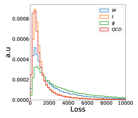
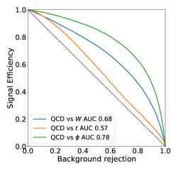
We compare the performance of our network with the particle graph autoencoders (PGAE) proposed in Ref. kasieczka2021lhc 666We use the code available in https://github.com/stsan9/AnomalyDetection4Jets/tree/rnd_cuts with our dataset. This study focussed on identifying anomalous events with dijet signatures (large-radius jets and high ) and used the two leading jets in the event to learn latent event representations. In contrast, our present focus is jet-level classification. For the input, we consider the four-vector of each microjet as the node feature and use a complete graph with all possible connections. The network is a graph-autoencoder that takes the vectors as input with a single edge convolution to map it to a two-dimensional latent node representation and maps it back with another single edge convolution. We use the mean squared error as the loss function and train with a batch size of 32. For more details of the architecture, we refer the reader to Section 3.7 of Ref. kasieczka2021lhc . We show the distribution of the loss function and the corresponding ROC curve in Fig. 8. The first thing that we notice is that the location of the peaks is identical for all four classes, with the only difference coming in the tail of the distribution. The value of the AUCs is significantly reduced for and top jets compared to our work, while for -jets, the reduction is not that drastic. Out of the three signal classes, jets are the least QCD-like, and hence, the networks find it easier to distinguish them with less information. At the same time, the edge-reconstruction employed in our architecture helps identify the and top jets more efficiently. Hence, we infer that the edge-reconstruction and the multidimensional edge feature representation is crucial for a graph-autoencoder as these complex and physically relevant features are not learned by the network even though they are, in principle, constructed from the node features. Moreover, using only the node features, the graph autoencoder is insensitive to the n-prong structure of the signals as the AUCs do not follow the usual QCD intuition. The addition of the edge features and their reconstruction enables the graph-autoencoder to learn the signal jets’ -prong topology in an unsupervised manner.
Appendix B Correlation of the loss function with jet variables
The correlation of the loss function with different jet variables is essential in determining the trained network’s biases. Although perfectly decorrelated discriminants to the jet’s physical variables like transverse momentum (), mass (), or the number of constituents are highly coveted, it is not possible in practice – known methods to decorrelate them, like adversarial training, diminish the power of the discriminant. We discuss the correlation of our network’s loss function with the quantities mentioned earlier in this section. The class-wise correlation of the four quantities is shown in Fig. 9. We see that the loss function and the are uncorrelated with small positive values (the highest being 0.27 for ), indicating that the loss function tends to increase with an increase in transverse momentum of the jet slightly, although the increase is minimal for the background QCD jets (). Jet mass is an important variable that helps in discriminating different classes of jets. However, a discriminant (the loss function) needs to be decorrelated entirely with jet mass as putting a cut on a correlated variable will lead to artificial bumps in the jet-mass distribution of the selected events. As can be seen, from Fig. 9, the loss function is reasonably correlated with the jet mass even for the QCD jets. Decorrelating the jet mass from the loss can be done via an adversarial network Heimel:2018mkt .
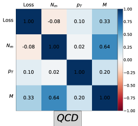
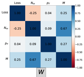
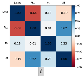
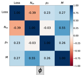
The reconstruction efficiency of convolutional autoencoders has been shown to decrease with an increase in the number of non-zero pixels Finke:2021sdf , which leads to the possibility of missing out on potential signals with lower complexities than QCD jets. We find that our network behaves in the opposite way: the reconstruction error reduces with an increase in the number of microjets. More importantly, this reduction is minimal for the QCD jets, suggesting that the network learns a uniform feature of the jet graph regardless of the number of microjets.
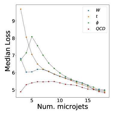
We can understand this independence via the structure of a graph neural network. A graph convolution layer essentially learns a set of weights shared for all the nodes and edges and hence learns the underlying feature regardless of the number of nodes/edges in the graphs. However, there is a strong negative correlation of the loss of the different signal classes with the number of microjets which can be understood via the fact that any extra radiation other than the said multiplicities essentially arise from QCD splittings. To further understand this behavior, we plot the median loss of the events with a fixed number of microjets for the four classes in Fig. 10. The initial increase in the median loss from three to five for the four-pronged jets further solidifies the preceding argument regarding the decrease of the loss function with an increase in the microjet multiplicity. Such a peak is absent for the lower multiplicity signal classes.
References
- (1) I. Brivio and M. Trott, The Standard Model as an Effective Field Theory, Phys. Rept. 793 (2019) 1–98, [1706.08945].
- (2) J. H. Collins, P. Martín-Ramiro, B. Nachman and D. Shih, Comparing Weak- and Unsupervised Methods for Resonant Anomaly Detection, 2104.02092.
- (3) CMS collaboration, A. M. Sirunyan et al., MUSiC: a model unspecific search for new physics in proton-proton collisions at 13 TeV, 2010.02984.
- (4) ATLAS collaboration, M. Aaboud et al., A strategy for a general search for new phenomena using data-derived signal regions and its application within the ATLAS experiment, Eur. Phys. J. C 79 (2019) 120, [1807.07447].
- (5) J. H. Collins, K. Howe and B. Nachman, Anomaly Detection for Resonant New Physics with Machine Learning, Phys. Rev. Lett. 121 (2018) 241803, [1805.02664].
- (6) A. Blance, M. Spannowsky and P. Waite, Adversarially-trained autoencoders for robust unsupervised new physics searches, JHEP 10 (2019) 047, [1905.10384].
- (7) J. Hajer, Y.-Y. Li, T. Liu and H. Wang, Novelty Detection Meets Collider Physics, Phys. Rev. D 101 (2020) 076015, [1807.10261].
- (8) A. De Simone and T. Jacques, Guiding New Physics Searches with Unsupervised Learning, Eur. Phys. J. C 79 (2019) 289, [1807.06038].
- (9) B. Nachman and D. Shih, Anomaly Detection with Density Estimation, Phys. Rev. D 101 (2020) 075042, [2001.04990].
- (10) B. Nachman, Anomaly Detection for Physics Analysis and Less than Supervised Learning, 2010.14554.
- (11) S. Marzani, G. Soyez and M. Spannowsky, Looking inside jets: an introduction to jet substructure and boosted-object phenomenology, 1901.10342.
- (12) D. E. Soper and M. Spannowsky, Finding physics signals with shower deconstruction, Phys. Rev. D84 (2011) 074002, [1102.3480].
- (13) D. E. Soper and M. Spannowsky, Finding physics signals with event deconstruction, Phys. Rev. D89 (2014) 094005, [1402.1189].
- (14) ATLAS collaboration, G. Aad et al., Measurements of the W production cross sections in association with jets with the ATLAS detector, Eur. Phys. J. C75 (2015) 82, [1409.8639].
- (15) J. Zhou, G. Cui, Z. Zhang, C. Yang, Z. Liu, L. Wang et al., Graph neural networks: A review of methods and applications, 1812.08434.
- (16) Z. Wu, S. Pan, F. Chen, G. Long, C. Zhang and P. S. Yu, A comprehensive survey on graph neural networks, IEEE Transactions on Neural Networks and Learning Systems 32 (2021) 4–24, [1901.00596].
- (17) F. A. Dreyer and H. Qu, Jet tagging in the Lund plane with graph networks, JHEP 03 (2021) 052, [2012.08526].
- (18) B. Andersson, G. Gustafson, L. Lonnblad and U. Pettersson, Coherence Effects in Deep Inelastic Scattering, Z. Phys. C43 (1989) 625.
- (19) A. Lifson, G. P. Salam and G. Soyez, Calculating the primary Lund Jet Plane density, JHEP 10 (2020) 170, [2007.06578].
- (20) V. Mikuni and F. Canelli, ABCNet: An attention-based method for particle tagging, Eur. Phys. J. Plus 135 (2020) 463, [2001.05311].
- (21) O. Knapp, O. Cerri, G. Dissertori, T. Q. Nguyen, M. Pierini and J.-R. Vlimant, Adversarially Learned Anomaly Detection on CMS Open Data: re-discovering the top quark, Eur. Phys. J. Plus 136 (2021) 236, [2005.01598].
- (22) V. Mikuni and F. Canelli, Unsupervised clustering for collider physics, 2010.07106.
- (23) G. Dezoort, S. Thais, I. Ojalvo, P. Elmer, V. Razavimaleki, J. Duarte et al., Charged particle tracking via edge-classifying interaction networks, 2103.16701.
- (24) M. Abdughani, J. Ren, L. Wu and J. M. Yang, Probing stop pair production at the LHC with graph neural networks, JHEP 08 (2019) 055, [1807.09088].
- (25) Y. Iiyama et al., Distance-Weighted Graph Neural Networks on FPGAs for Real-Time Particle Reconstruction in High Energy Physics, Front. Big Data 3 (2020) 598927, [2008.03601].
- (26) M. Farina, Y. Nakai and D. Shih, Searching for New Physics with Deep Autoencoders, Phys. Rev. D 101 (2020) 075021, [1808.08992].
- (27) T. Heimel, G. Kasieczka, T. Plehn and J. M. Thompson, QCD or What?, SciPost Phys. 6 (2019) 030, [1808.08979].
- (28) T. S. Roy and A. H. Vijay, A robust anomaly finder based on autoencoders, 1903.02032.
- (29) C. K. Khosa and V. Sanz, Anomaly Awareness, 2007.14462.
- (30) T. Finke, M. Krämer, A. Morandini, A. Mück and I. Oleksiyuk, Autoencoders for unsupervised anomaly detection in high energy physics, 2104.09051.
- (31) T. Cheng, J.-F. Arguin, J. Leissner-Martin, J. Pilette and T. Golling, Variational Autoencoders for Anomalous Jet Tagging, 2007.01850.
- (32) J. Cogan, M. Kagan, E. Strauss and A. Schwarztman, Jet-Images: Computer Vision Inspired Techniques for Jet Tagging, JHEP 02 (2015) 118, [1407.5675].
- (33) L. de Oliveira, M. Kagan, L. Mackey, B. Nachman and A. Schwartzman, Jet-images — deep learning edition, JHEP 07 (2016) 069, [1511.05190].
- (34) X. Ju and B. Nachman, Supervised Jet Clustering with Graph Neural Networks for Lorentz Boosted Bosons, Phys. Rev. D102 (2020) 075014, [2008.06064].
- (35) H. Qu and L. Gouskos, ParticleNet: Jet Tagging via Particle Clouds, Phys. Rev. D 101 (2020) 056019, [1902.08570].
- (36) A. Blance and M. Spannowsky, Unsupervised Event Classification with Graphs on Classical and Photonic Quantum Computers, 2103.03897.
- (37) G. Kasieczka, B. Nachman, D. Shih, O. Amram, A. Andreassen, K. Benkendorfer et al., The lhc olympics 2020: A community challenge for anomaly detection in high energy physics, 2101.08320.
- (38) T. N. Kipf and M. Welling, Variational graph auto-encoders, 1611.07308.
- (39) P. V. Tran, Learning to make predictions on graphs with autoencoders, in 2018 IEEE 5th international conference on data science and advanced analytics (DSAA), pp. 237–245, IEEE, 2018. 1802.08352.
- (40) G. Salha, R. Hennequin and M. Vazirgiannis, Simple and effective graph autoencoders with one-hop linear models, 2001.07614.
- (41) S. Pan, R. Hu, G. Long, J. Jiang, L. Yao and C. Zhang, Adversarially regularized graph autoencoder for graph embedding, 1802.04407.
- (42) J. Park, M. Lee, H. J. Chang, K. Lee and J. Y. Choi, Symmetric graph convolutional autoencoder for unsupervised graph representation learning, in Proceedings of the IEEE/CVF International Conference on Computer Vision, pp. 6519–6528, 2019. 1908.02441.
- (43) J. Alwall, R. Frederix, S. Frixione, V. Hirschi, F. Maltoni, O. Mattelaer et al., The automated computation of tree-level and next-to-leading order differential cross sections, and their matching to parton shower simulations, JHEP 07 (2014) 079, [1405.0301].
- (44) T. Sjostrand, S. Mrenna and P. Z. Skands, PYTHIA 6.4 Physics and Manual, JHEP 05 (2006) 026, [hep-ph/0603175].
- (45) M. Cacciari, G. P. Salam and G. Soyez, The anti- jet clustering algorithm, JHEP 04 (2008) 063, [0802.1189].
- (46) M. Cacciari, G. P. Salam and G. Soyez, FastJet User Manual, Eur. Phys. J. C72 (2012) 1896, [1111.6097].
- (47) ATLAS collaboration, “Performance of shower deconstruction in ATLAS.” http://cdsweb.cern.ch/record/1648661, 2, ATLAS-CONF-2014-003.
- (48) S. Catani, Y. L. Dokshitzer, M. Olsson, G. Turnock and B. R. Webber, New clustering algorithm for multi - jet cross-sections in e+ e- annihilation, Phys. Lett. B269 (1991) 432–438.
- (49) S. D. Ellis and D. E. Soper, Successive combination jet algorithm for hadron collisions, Phys. Rev. D48 (1993) 3160–3166, [hep-ph/9305266].
- (50) M. Wang, D. Zheng, Z. Ye, Q. Gan, M. Li, X. Song et al., Deep graph library: A graph-centric, highly-performant package for graph neural networks, 1909.01315.
- (51) A. Paszke, S. Gross, F. Massa, A. Lerer, J. Bradbury, G. Chanan et al., Pytorch: An imperative style, high-performance deep learning library, 1912.01703.
- (52) Y. Lecun, L. Bottou, Y. Bengio and P. Haffner, Gradient-based learning applied to document recognition, Proceedings of the IEEE 86 (1998) 2278–2324.
- (53) J. Gilmer, S. S. Schoenholz, P. F. Riley, O. Vinyals and G. E. Dahl, Neural message passing for quantum chemistry, in International Conference on Machine Learning, pp. 1263–1272, PMLR, 2017. 1704.01212.
- (54) Y. Wang, Y. Sun, Z. Liu, S. E. Sarma, M. M. Bronstein and J. M. Solomon, Dynamic graph cnn for learning on point clouds, Acm Transactions On Graphics (tog) 38 (2019) 1–12, [1801.07829].
- (55) D. P. Kingma and J. Ba, Adam: A method for stochastic optimization, 1412.6980.
- (56) B. M. Dillon, D. A. Faroughy, J. F. Kamenik and M. Szewc, Learning the latent structure of collider events, Journal of High Energy Physics 2020 (Oct, 2020) .
- (57) B. Bortolato, B. M. Dillon, J. F. Kamenik and A. Smolkovič, Bump hunting in latent space, 2103.06595.
- (58) B. M. Dillon, T. Plehn, C. Sauer and P. Sorrenson, Better latent spaces for better autoencoders, 2104.08291.
- (59) D. P. Kingma and M. Welling, Auto-encoding variational bayes, 1312.6114.
- (60) A. Makhzani, J. Shlens, N. Jaitly, I. Goodfellow and B. Frey, Adversarial autoencoders, 1511.05644.
- (61) G. Patrini, R. van den Berg, P. Forré, M. Carioni, S. Bhargav, M. Welling et al., Sinkhorn autoencoders, 1810.01118.