Polarized Z bosons from the decay of a Higgs boson produced in association with two jets at the LHC

Abstract

Investigating the polarization of weak bosons provides an important probe of the scalar and gauge sector of the Standard Model. This can be done in the Higgs decay to four leptons, whose Standard-Model leading-order amplitude enables to generate polarized observables from unpolarized ones via a fully-differential reweighting method. We study the Z-boson polarization from the decay of a Higgs boson produced in association with two jets, both in the gluon-fusion and in the vector-boson fusion channel. We also address the possibility of extending the results of this work to higher orders in perturbation theory.

1 Introduction

The discovery of the Higgs boson Chatrchyan:2012xdj ; Aad:2012tfa has enabled a large number of tests of the Standard Model (SM) scalar and gauge sectors.

In the SM, electroweak bosons (W and Z) acquire their mass and, as a consequence, an additional longitudinal polarization, through their coupling to the Higgs field. Therefore the interplay between the Higgs boson and weak-boson polarizations represents a crucial probe for the SM electroweak symmetry breaking mechanism as well as an ideal framework for searches of possible modifications due to new-physics effects.

The gold-plated channel for these searches is given by vector-boson scattering (VBS), as in the high-energy regime the unitarity-violating behaviour of the scattering among longitudinal bosons is regularized by the inclusion of Higgs exchange contributions Dicus:1992vj ; LlewellynSmith:1973yud ; Veltman:1976rt . Studying the Higgs coupling to polarized weak bosons can provide relevant insight also at the Higgs-boson resonance itself Brehmer:2014pka , in particular with the aim of discriminating between the SM and models with modified Higgs sectors. Since vector-boson polarizations are best accessed through the angular distribution of their decay products, the cleanest channel is the Higgs decay to four charged leptons.

The Higgs-boson decay into four charged leptons has been widely studied by the ATLAS and CMS experimental collaborations with Run-1 (7 and 8 TeV) and Run-2 data (13 TeV), with the purpose of determining the Higgs-boson mass Chatrchyan:2013mxa ; Aad:2014eva ; Sirunyan:2017exp and width Khachatryan:2014iha ; Khachatryan:2015mma ; Sirunyan:2019twz , its spin and parity properties Chatrchyan:2013mxa ; Khachatryan:2014kca ; Aaboud:2017vzb ; Aad:2020mkp , the inclusive and differential cross-sections Aad:2014tca ; Khachatryan:2015yvw ; Aaboud:2017oem ; Aaboud:2017vzb ; Aad:2020mkp ; ATLAS:2020wny ; Sirunyan:2021rug , and the Higgs coupling to weak bosons in the on-shell and off-shell regions Khachatryan:2014kca ; Aaboud:2017vzb ; Sirunyan:2017tqd ; Aaboud:2018puo ; Sirunyan:2019twz ; Sirunyan:2021fpv . So far, all measurements are compatible with the SM predictions. This decay channel features a large signal-to-background ratio, thanks to the possibility to fully reconstruct the decay products and to small background contributions.

The four-lepton Higgs-boson decay has been extensively investigated also from a theoretical point of view, providing a very precise characterisation of the scalar boson properties. The SM decay of a Higgs boson into four leptons is known perturbatively up to next-to-leading order (NLO) in the electroweak (EW) coupling Bredenstein:2006rh and has been matched to QED parton-showers Boselli:2015aha . This decay channel has been computed at EW NLO also for beyond-the-SM theories with modified Higgs sectors Altenkamp:2018bcs ; Altenkamp:2018hrq ; Kanemura:2019kjg , and has been investigated within an effective-field-theory framework Artoisenet:2013puc ; Boselli:2017pef ; Brivio:2019myy . Spin effects, angular and energy correlations have been widely studied Soni:1993jc ; Chang:1993jy ; Skjold:1993jd ; Arens:1994wd ; Buszello:2002uu ; Choi:2002jk ; Hagiwara:2009wt ; Gao:2010qx ; Bolognesi:2012mm ; Berge:2015jra .

At the Large Hadron Collider (LHC), the Higgs boson is mostly produced in the gluon-fusion (GGF) and in the vector-boson-fusion (VBF) channels. Experimental analyses can be either inclusive or exclusive in the production mode of the Higgs boson, depending on the specific target of the investigation. For the purposes of this work, we only consider the production of a Higgs boson in association with two jets. In this channel the GGF and VBF contributions are comparable. The SM prediction for an on-shell Higgs boson produced in GGF in association with two jets is known at leading order (LO) in QCD, including also dependence on the top-quark mass DelDuca:2001eu ; DelDuca:2001fn ; Greiner:2016awe . Predictions in the large-$m_{\text{t}}$ limit are known up to NLO QCD Cullen:2013saa . The full mass dependence has also been studied in the presence of high-energy jets Andersen:2018kjg . The predictions for VBF are known at NLO QCD+EW accuracy Ciccolini:2007jr , and up to $\rm N^{3}LO$ QCD Dreyer:2016oyx in the structure-function approximation Han:1992hr . It has been shown DelDuca:2001eu ; DelDuca:2001fn that for an on-shell Higgs produced in GGF in association with two jets, the large-$m_{\text{t}}$ approximation gives a very good description of the loop-induced SM process with full $m_{t}$ dependence, of order $\mathcal{O}(\alpha_{\text{s}}^{4}\alpha)$, provided that the transverse-momenta of jets and the Higgs-boson mass are smaller than the top-quark mass. The logarithmic structure of Higgs production in association with up to two jets and the kinematic configurations where finite top-mass effects become relevant are also known Buschmann:2014twa ; Buschmann:2014sia . The large-$m_{\text{t}}$ approximation works well also in the presence of a two-jet system with large invariant mass DelDuca:2001eu ; DelDuca:2001fn ; Campbell:2012am , which is the typical VBF phase-space region. The interference between VBF and GGF signals has been proved to be negligible Andersen:2007mp .

The phenomenology of weak-boson polarizations has been widely investigated both in experimental analyses and in theoretical studies.

The ATLAS and CMS collaborations have measured final-state vector-boson polarizations (typically using the leptonic decay channel) in several multi-boson processes in 8 and 13 TeV hadronic collisions, including $V$+jets Chatrchyan:2011ig ; ATLAS:2012au ; Khachatryan:2015paa ; Aad:2016izn , di-boson production Aaboud:2019gxl and vector-boson scattering Sirunyan:2020gvn . Polarizations have also been measured for W bosons produced in top-quark decays Aaboud:2016hsq ; Khachatryan:2016fky ; Aad:2020jvx , as well as for $V$ bosons produced in Higgs-boson decays, ${\rm h}\rightarrow VV^{*}$ Aaboud:2018jqu ; Bruni:2019xwu . Enhanced sensitivity to polarizations is expected in the forthcoming high-luminosity and high-energy LHC runs CMS-PAS-FTR-18-014 ; Azzi:2019yne .

From the theory side, the W-boson polarization at the LHC has been studied in ref. Bern:2011ie in the absence of lepton cuts. Realistic selection cuts has been introduced in ref. Stirling:2012zt both in $V+{}$jets and in other multi-boson production processes. The interference between amplitudes for different polarizations has been investigated in ref. Belyaev:2013nla .

In ref. Ballestrero:2017bxn a simple and natural method to define cross sections corresponding to vector bosons of definite polarization has been proposed. This method has been applied to study the polarization of W and Z bosons in vector-boson scattering at LO Ballestrero:2017bxn ; Ballestrero:2019qoy ; Ballestrero:2020qgv and in di-boson production at NLO QCD Denner:2020bcz ; Denner:2020eck with purely leptonic final states. Polarizations in $\text{W}^{\pm}\text{Z}$ production, including NLO QCD and EW corrections have been analyzed in refs. Baglio:2018rcu ; Baglio:2019nmc . Recently MadGraph has introduced the possibility of generating polarized amplitudes BuarqueFranzosi:2019boy . Ref. Cao:2020npb has suggested that a study of vector-boson polarizations in gluon-induced ZZ production could be sensitive to the $\text{Z}\text{t}\bar{\text{t}}$ coupling.

A study of the vector-boson polarization effects at the Higgs resonance in VBF has been performed in the $\text{W}^{+}\text{W}^{-}$ channel, using effective Higgs couplings to longitudinal and transverse bosons and including a general dimension-six EFT interpretation Brehmer:2014pka . The possibility of measuring the coupling of the Higgs to polarized bosons is studied in ref. Bruni:2019xwu .

In this work we perform a phenomenological study of polarized electroweak bosons from the decay of a SM Higgs boson produced in association with two jets at the LHC. In ref. Maina:2020rgd a first assessment of polarized bosons from Higgs decays has been performed in the LO production of a Higgs in gluon fusion, that is, for a Higgs with vanishing transverse momentum. In this paper we consider the case in which the Higgs boson is produced in association with two jets, both in VBF and in GGF. Although the focus is on the Higgs signals, a number of comments are made concerning the impact of the QCD background and of the pure electroweak contributions to VBF.

The phenomenological analysis is limited to the four-lepton Higgs decay, with two pairs of opposite-charge leptons and different flavours. Despite a very small cross-section, due to the small branching ratio, the considered decay channel has two advantages. First, it enables the complete reconstruction of the Higgs-boson kinematics, thanks to the absence of neutrinos in the final state. Second, it allows for an unambiguous determination of the kinematics of each Z-boson, thanks to the different lepton flavours.

VBF and GGF Higgs production with two jets has already been widely investigated Klamke:2007cu ; Andersen:2008gc ; Andersen:2012kn ; Demartin:2014fia , mostly with the purpose of finding kinematic regimes and observables that discriminate between the two signals. In this work, however, we do not aim to separate the Higgs signals, instead, we address the possibility to perform a polarization study of vector bosons in Higgs decay, rather independently of the Higgs-production mechanism. Given the very small fraction of Higgs bosons decaying into four charged leptons, being able to sum over different production channels is crucial to enhance the experimental sensitivity to the polarization structure.

As a last comment, we choose to work in the large-$m_{\text{t}}$ limit for the GGF signal. Given the purposes of this work, it represents a satisfactory approximation.

This paper is organised as follows. In Sect. 2 we show the details of the matrix-element reweighting method that we use to generate polarized cross-sections and distributions. The fiducial setup we employ for numerical simulations is given in Sect. 4. In Sect. 5 we validate the reweighting technique comparing its results with those obtained directly simulating polarized events Ballestrero:2017bxn . The polarized results for VBF and GGF signals are shown and discussed in Sect. 6. In Sect. 7 we draw our conclusions.

2 Matrix-element reweighting

In Fig. 1 we show the general structure of Higgs-mediated amplitudes contributing to a reaction producing the Higgs-decay products (four charged-leptons) and an arbitrary number of jets.

We notice that these amplitudes (which we call signal contributions) are only a sub-set of all amplitudes for the production of four charged leptons in association with jets. Therefore, they are not gauge invariant per sè. Nonetheless, we have checked numerically that with a sharp but realistic cut on the invariant mass of the four leptons, e.g. $|M_{4\ell}-M_{\rm h}|<5\,\text{GeV}$, the $s$-channel Higgs contributions are largely dominant and sufficient to describe the full-matrix-element calculation up to few-permille effects.

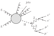
Figure 1: General structure of the Standard Model amplitude for the production of a Higgs boson (decaying into four charged leptons) in association with jets.

We observe that for this work it is important that the Higgs-decay products can be unambiguously identified and distinguished from the additional jets produced in association with the Higgs boson in order to minimize the impact of irreducible backgrounds and reconstruction effects.

Provided we define vector-boson polarizations in the Higgs rest frame, we can easily parametrize the Higgs-decay amplitude as a sum of polarized and interference terms Maina:2020rgd :

$$|\mathcal{A}^{\rm SM}_{h\rightarrow\text{Z}\text{Z}}|^{2} = \Big{[}|\mathcal{A}_{{\mathrm{L}}{\mathrm{L}}}|^{2}+|\mathcal{A}_{++}|^{2}+|\mathcal{A}_{--}|^{2}$$ (1)

$$+2\,{\rm Re}(\mathcal{A_{{\mathrm{L}}{\mathrm{L}}}}^{\!*}\mathcal{A}_{++})+2\,{\rm Re}(\mathcal{A_{{\mathrm{L}}{\mathrm{L}}}}^{\!*}\mathcal{A}_{--})$$

$$+2\,{\rm Re}(\mathcal{A_{++}}^{\!*}\mathcal{A}_{--})\,\Big{]}$$

where the first three terms in the sum correspond to a definite polarization state $\lambda$ for both bosons, longitudinal ($\lambda={\rm L}$), right-handed ($\lambda=+$) and left-handed ($\lambda=-$), while the fourth and fifth terms are contributions from longitudinal-transverse interference, and the last one comes from left-right interference. Note that, since polarization vectors are defined in the Higgs-boson rest frame there are no mixed-state contributions, i.e. $\mathcal{A}_{\lambda\lambda^{\prime}}=0$ for $\lambda\neq\lambda^{\prime}$. The analytic expression for each term of the sum of Eq. 1 reads

$$|\mathcal{A}_{{\mathrm{L}}{\mathrm{L}}}|^{2} = 4\,K^{2}\,P(Q_{1})\,P(Q_{2})\,$$

$$\times \left(c_{L}^{2}+c_{R}^{2}\right)^{2}\,\sin^{2}\theta^{*}_{1}\,\sin^{2}\theta^{*}_{2}$$

$$|\mathcal{A}_{++}|^{2} = \,P(Q_{1})\,P(Q_{2})\,$$

$$\times \Big{[}\,c_{L}^{4}\,(1+\cos\theta^{*}_{1})^{2}\,(1+\cos\theta^{*}_{2})^{2}$$

$$+c_{R}^{4}\,(1-\cos\theta^{*}_{1})^{2}\,(1-\cos\theta^{*}_{2})^{2}$$

$$+c_{R}^{2}c_{L}^{2}\,(1+\cos\theta^{*}_{1})^{2}\,(1-\cos\theta^{*}_{2})^{2}$$

$$+c_{R}^{2}c_{L}^{2}\,(1-\cos\theta^{*}_{1})^{2}\,(1+\cos\theta^{*}_{2})^{2}\,\Big{]}$$

$$|\mathcal{A}_{--}|^{2} = \,P(Q_{1})\,P(Q_{2})\,$$

$$\times \Big{[}\,c_{L}^{4}\,(1-\cos\theta^{*}_{1})^{2}\,(1-\cos\theta^{*}_{2})^{2}$$

$$+c_{R}^{4}\,(1+\cos\theta^{*}_{1})^{2}\,(1+\cos\theta^{*}_{2})^{2}$$

$$+c_{R}^{2}c_{L}^{2}\,(1+\cos\theta^{*}_{1})^{2}\,(1-\cos\theta^{*}_{2})^{2}$$

$$+c_{R}^{2}c_{L}^{2}\,(1-\cos\theta^{*}_{1})^{2}\,(1+\cos\theta^{*}_{2})^{2}\,\Big{]}$$

$$2\,{\rm Re}(\mathcal{A_{{\mathrm{L}}{\mathrm{L}}}}^{\!*}\mathcal{A}_{++}) = \,-4\,K\,P(Q_{1})\,P(Q_{2})\,$$

$$\times \Big{[}\,c_{L}^{4}\,(1+\cos\theta^{*}_{1})\,(1+\cos\theta^{*}_{2})$$

$$+c_{R}^{4}\,(1-\cos\theta^{*}_{1})\,(1-\cos\theta^{*}_{2})$$

$$-c_{R}^{2}c_{L}^{2}\,(1+\cos\theta^{*}_{1})\,(1-\cos\theta^{*}_{2})$$

$$-c_{R}^{2}c_{L}^{2}\,(1-\cos\theta^{*}_{1})\,(1+\cos\theta^{*}_{2})\,\Big{]}$$

$$\times \sin\theta^{*}_{1}\,\sin\theta^{*}_{2}\,\cos\Delta\phi^{*}_{12}$$

$$2\,{\rm Re}(\mathcal{A_{{\mathrm{L}}{\mathrm{L}}}}^{\!*}\mathcal{A}_{--}) = \,-4\,K\,P(Q_{1})\,P(Q_{2})\,$$

$$\times \Big{[}\,c_{L}^{4}\,(1-\cos\theta^{*}_{1})\,(1-\cos\theta^{*}_{2})$$

$$+c_{R}^{4}\,(1+\cos\theta^{*}_{1})\,(1+\cos\theta^{*}_{2})$$

$$-c_{R}^{2}c_{L}^{2}\,(1+\cos\theta^{*}_{1})\,(1-\cos\theta^{*}_{2})$$

$$-c_{R}^{2}c_{L}^{2}\,(1-\cos\theta^{*}_{1})\,(1+\cos\theta^{*}_{2})\,\Big{]}$$

$$\times \sin\theta^{*}_{1}\,\sin\theta^{*}_{2}\,\cos(\Delta\phi^{*}_{12})$$

$$2\,{\rm Re}(\mathcal{A_{++}}^{\!*}\mathcal{A}_{--}) = \,2\,P(Q_{1})\,P(Q_{2})\,$$

$$\times\,\left(c_{L}^{2}+c_{R}^{2}\right)^{2}\,\sin^{2}\theta^{*}_{1}\,\sin^{2}\theta^{*}_{2}\,\cos(2\Delta\phi^{*}_{12})\,.$$

In Eqs. 2–2 we have defined the $P(Q_{i})$ propagator factor as

$$P(Q_{i})\,=\,\frac{2\,g_{{\scalebox{0.6}{\rm hZZ}}}\,Q_{i}^{2}}{\left(Q_{i}^{2}-M_{\text{Z}}^{2}\right)^{2}+\Gamma_{\text{Z}}^{2}M_{\text{Z}}^{2}}\,,$$ (8)

depending on the Higgs-to-gauge-boson coupling ($g_{\rm{\scalebox{0.6}{\rm hZZ}}}$), the Z pole mass and width, and the invariant mass of the $i$-th Z boson ($Q_{i}$). We have also introduced the factor

$$K=\frac{Q^{2}-Q_{1}^{2}-Q_{2}^{2}}{2\,Q_{1}\,Q_{2}}\,,$$ (9)

where $Q$ is the Higgs-boson invariant mass. The $c_{L},c_{R}$ parameters represent the SM left- and right-chirality coupling of the Z boson to massless leptons. The variables $\theta^{*}_{1(2)},\phi^{*}_{1(2)}$ are the positively-charged-lepton decay angles computed in the corresponding Z-boson rest frame, with respect to the boson flight direction in the Higgs rest frame, and $\Delta\phi^{*}_{12}=\phi^{*}_{1}-\phi^{*}_{2}$.

Instead of considering the left-handed and right-handed contributions separately, we combine them in a single transverse (T) contribution which includes also the left-right interference term,

$$|\mathcal{A}_{{\mathrm{T}}{\mathrm{T}}}|^{2}=|\mathcal{A}_{++}|^{2}+|\mathcal{A}_{--}|^{2}+2\,{\rm Re}(\mathcal{A_{++}}^{\!*}\mathcal{A}_{--})\,.$$ (10)

The definition of the transverse mode as a coherent sum of the left and right modes minimizes the interference effects, which now come only from longitudinal-transverse terms in Eqs. 2-2. Moreover, it is known Maina:2020rgd that in the Higgs decay to four charged leptons the longitudinal-transverse interference is only a few percent of the total result, much smaller than the interference between the right and left amplitudes included in Eq. 10. Introducing the following longitudinal or transverse weights,

$$w_{\lambda}=\frac{\big{|}\mathcal{A}_{\lambda\lambda}\big{|}^{2}}{\big{|}\mathcal{A}^{\rm SM}_{h\rightarrow\text{Z}\text{Z}}\big{|}^{2}}\,,\quad\lambda={\mathrm{L}},{\mathrm{T}}\,,$$ (11)

it is possible to compute any polarized distribution, with arbitrary cuts on the lepton kinematics, multiplying the weight of each unpolarized event by the factor in Eq. 11. In this way it becomes unnecessary to generate separately the individual polarized contributions. All the subtleties related to sampling events with negative weights are avoided.

We stress that this procedure is accurate only because of the special (and relatively simple) Higgs-decay analytic structure. Applying the same approach to general multi-boson processes would require building weights that depend on non-factorized amplitudes, which would be much more time-consuming and equivalent to directly generate events with polarized amplitudes.

This method is designed for the LO Higgs decay into four leptons. However, it could be extended to NLO, provided that it is possible to disentangle polarized contributions to the Z boson propagators. The NLO QCD corrections would only affect the production mechanism, therefore this entire formalism can be extended with no modifications to this perturbative order. However, we do not include QCD radiative corrections to the specific production processes that are considered in this paper, as this would not affect the main results of this work. The extension of this reweighting method to NLO EW corrections is more involved, in particular for the virtual contributions. These corrections are of the order of 2% Bredenstein:2006rh . The description of weak boson polarizations is not trivial if EW corrections are included, since a standard narrow-width or double-pole approximation Denner:2000bj is not viable for vector bosons from a 125-GeV Higgs-boson decay. Below the $2M_{\rm V}$ threshold the NLO EW corrections can be computed via an improved-Born approximation Denner:2019vbn , which is only valid for $M_{\rm VV}\approx 2M_{\rm V}-n\Gamma_{\rm V}$, with $n=2\div 3$. However, a rigorous description of weak boson polarizations in Higgs decay at NLO EW is possible in the single-pole approximation, namely projecting on mass shell only one of the two vector bosons. This is discussed in Sect. 3.

3 Single-pole approximation

In this section we briefly address the possibility of studying Z boson polarizations in Higgs decay including NLO EW effects. The presence of non-factorizable corrections both in the real and the virtual contributions makes the separation of polarizations of off-shell Z bosons not well defined, as several diagram topologies do not feature two $s$-channel Z-boson propagators. Such diagrams cannot be simply dropped as the result would not be gauge invariant. The pole approximation Stuart:1991xk ; Aeppli:1993rs can help in addressing this issue. Since on the Higgs resonance one of the two Z bosons is off its mass shell, it is only possible to project on-shell one of the two bosons. This method consists in:

• selecting only diagrams which feature at least a resonant Z boson decaying into two leptons,

• projecting the momenta of the $s$-channel Z-boson decay products such that their sum gives the momentum of an on-shell Z momentum,

• computing the numerator of the amplitude with the on-shell-projected kinematics, while evaluating the denominator with the original kinematics, to retain the Breit-Wigner modulation of an off-shell Z boson.

The method is accurate in the vicinity of the resonance pole mass Stuart:1991xk ; Aeppli:1993rs ; Denner:2019vbn , and is characterized by an intrinsic uncertainty of order $\mathcal{O}(\Gamma_{\text{Z}}/M_{\text{Z}})\approx\mathcal{O}(\alpha)$. This procedure requires a careful treatment of non-factorizable QED corrections Denner:1997ia ; Dittmaier:2015bfe ; Denner:2019vbn , because of spurious infrared singularities that arise when setting the Z-boson momentum on its mass shell. Furthermore, the presence of photon contributions in the virtual corrections makes it essential to constrain the decay leptons to have an invariant mass that is as close as possible to the Z pole mass. This requirement has the advantage of making the Z-resonant contributions more dominant over the non-resonant ones, giving a more accurate pole-approximated description of the process. This induces the loss of signal events, due to the tighter constraint on the two leptons decaying from the almost-on-shell Z boson. We have calculated that with realistic kinematic selections (see LEP setup of Sect. 4), the additional constraint $|M_{\text{e}^{+}\text{e}^{-}}-M_{\text{Z}}|<5\,\text{GeV}$ reduces the VBF total cross-section by 70%. Most of the effect comes from the fact that only half of the events contain an almost-on-shell $\text{e}^{+}\text{e}^{-}$ pair. However, one should include also the contribution from almost-on-shell $\mu^{+}\mu^{-}$ pairs.

The choice of the specific on-shell projection is not unique Denner:2000bj ; Ballestrero:2017bxn ; Ballestrero:2019qoy ; Denner:2019vbn , and introduces an artificial modification of the momenta, which depends on the physical quantities that one chooses to conserve. In Higgs decay, the choice of such a projection is even more delicate than in other processes, as changing the momenta of one Z boson could induce a shift in the total momentum of the Higgs boson itself, resulting in a bad phase-space sampling in the region of the Higgs resonance and in large discrepancies w.r.t. the full calculation. Therefore, an essential requirement for the on-shell projection is to preserve the total momentum of the four leptons. A viable projection for the process $\rm h\rightarrow\text{Z}_{1}(\rightarrow\text{e}^{+}\text{e}^{-})\,\text{Z}^{*}_{2}(\rightarrow\mu^{+}\mu^{-})$ preserves:

• the spatial direction of $\text{e}^{\pm}$ in the rest frame of the $\text{e}^{+}\text{e}^{-}$ system,

• the spatial direction of $\mu^{\pm}$ in the rest frame of the $\mu^{+}\mu^{-}$ system,

• the spatial direction of the $\text{e}^{+}\text{e}^{-}$ system in the rest frame of the four-lepton system,

• the invariant mass of the $\mu^{+}\mu^{-}$ system,

• the four-momentum of the four-lepton system.

This choice preserves the decay angles of the leptons in the corresponding Z-boson rest frame, minimizing the effect of the pole approximation on polarization-sensitive variables. This specific on-shell projection only works if the invariant mass of the Higgs boson is larger than the sum $M_{\text{Z}}+M_{\mu^{+}\mu^{-}}$, giving a decrease in the total cross-section, which is of the same order of magnitude as the intrinsic uncertainty of the pole approximation.

This approach, despite some technical details which must be properly taken care of, is expected to give a reliable description of the Higgs-boson decay into four leptons at NLO EW, in the case where one of the two lepton pairs is close to the Z-boson mass shell. The single-pole approximation allows to select in a gauge invariant way only resonant contributions and therefore to reliably separate the polarizations of a single boson at the amplitude level. Since in the SM the Higgs couples to two weak bosons with like-wise polarization mode, selecting the polarization mode of the on-shell Z boson intrinsically gives important information about the polarization of the off-shell boson, which can be then studied by means of the usual angular observables of its decay leptons.

We conclude that the single-pole approximation represents a viable procedure to extend the LO polarization studies on the Higgs resonance to higher orders, in particular for NLO EW corrections. We leave this for future investigations.

4 Setup

We now proceed to the results for the parton-level process

$$\text{p}\,\text{p}\rightarrow\text{j}\,\text{j}\,{\rm h}(\rightarrow\text{e}^{+}\text{e}^{-}\mu^{+}\mu^{-})\,,$$ (12)

at the LHC with 13 TeV centre-of-mass energy. We have computed VBF and GGF signals at LO, the former simulated in the SM, the latter in the large-$m_{\text{t}}$ approximation, with the same numerical setup. A unit CKM matrix is assumed in both processes. We use NNPDF3.0 parton distribution functions (PDF) Ball:2014uwa computed at LO with $\alpha_{\text{s}}(M_{\text{Z}})=0.118$, via the LHAPDF interface Buckley:2014ana . The complex-mass scheme Denner:2005fg ; Denner:2006ic is understood for the treatment of electroweak-boson masses and couplings in the SM. The pole masses and widths of weak bosons and of the Higgs are set to the following values:

$$M_{\text{W}} = 80.358\,\text{GeV}\,,\qquad\Gamma_{\text{W}}=2.084\,\text{GeV}\,,$$

$$M_{\text{Z}} = 91.153\,\text{GeV}\,,\qquad\,\,\Gamma_{\text{Z}}=2.494\,\text{GeV}\,,$$

$$M_{\rm h} = 125\,\text{GeV}\,,\qquad\,\,\,\quad\Gamma_{\rm h}\,=\,4.07{\,\rm MeV}\,.$$ (13)

The electroweak coupling $\alpha$ is computed in the $G_{\mu}$ scheme, with the Fermi constant set to $G_{\mu}=1.16637\cdot 10^{-5}\,\text{GeV}^{-2}$. For both GGF and VBF, we work in the five-flavour scheme, i.e. including partonic processes with external massless b-quarks. These contributions account for less than 2% of the total cross-section.

We use a dynamical factorization and renormalization scale,

$$\mu_{\rm F}=\mu_{\rm R}=\sqrt{p_{{\mathrm{T}},{j_{1}}}p_{{\mathrm{T}},{j_{2}}}}\,,$$ (14)

that is a typical choice for GGF production DelDuca:2001eu ; DelDuca:2001fn . We have verified that the typical scale choice used for on-shell Higgs production Cacciari:2015jma gives results for VBF which differ by a few percent (both at the integrated and differential level) from those obtained with the dynamical choice in Eq. 14. We stress that the scale choice does not affect the main results of our work, as the reweighting procedure detailed in Sect. 2 is independent of the Higgs-production mechanism and its corresponding central-scale choice. We have employed two different setups.
The first setup (label INC) is inclusive in lepton kinematics, and is used for validation purposes:

• jets with minimum tranverse momentum $p_{{\mathrm{T}},{j}}>25\,\text{GeV}$ and maximum pseudo-rapidity $|\eta_{j}|<4.5$;

• a two-jet system with rather large invariant mass, $M_{\text{j}\text{j}}>300\,\text{GeV}$, large pseudo-rapidity separation, $|\Delta\eta_{\rm jj}|>2.5$, and such that $\eta_{j_{1}}\cdot\eta_{j_{2}}<0$;

• a four-lepton invariant mass close to the Higgs pole mass, $|M_{4\ell}-M_{\rm h}|<5\,\text{GeV}$;

• two pairs of opposite-charge leptons of different flavours, with $M_{\ell^{+}\ell^{-}}>10\,\text{GeV}$, for $\ell=\text{e},\mu$.

The requirements on the leading-jet pair are somewhat milder than those used for on-shell Higgs production in VBF Cacciari:2015jma and slightly stronger than those used in ZZ scattering studies Denner:2020zit .

The second setup (label LEP) includes, in addition to the ones of the INC setup, the following cuts on the lepton kinematics:

• for all charged leptons, $p_{{\mathrm{T}},{\ell^{\pm}}}>20\,\text{GeV}$, $|\eta_{\ell^{\pm}}|<2.5$.

Note that the effect of the lepton $p_{\rm T}$ and $\eta$ cuts is dramatic, as they decrease the signal cross-section roughly by a factor of 10, with respect to the INC setup. These cuts are the same used in the study of polarized Z-boson scattering performed in ref. Ballestrero:2019qoy . In recent experimental results on Higgs decay to four charged leptons Aad:2021ebo ; Sirunyan:2021rug the fiducial lepton cuts are slightly looser than those used in this work, therefore we expect a milder effect on polarized results in a realistic experimental analysis than in the present phenomenological setup.

For the simulation of the unpolarized VBF signal we have used the Phantom Monte Carlo Ballestrero:2007xq , which enables the selection of diagrams with an $s$-channel Higgs exchange from the complete set of tree-level, electroweak diagrams in the SM Ballestrero:2015jca . The same process has been simulated also with MadGraph Alwall:2014hca , with an agreement to better than 0.5% both in the total cross-section and in all analyzed differential distributions. The GGF signal has been simulated with MadGraph (version 2.7.3 BuarqueFranzosi:2019boy ), in the large-$m_{\text{t}}$ approximation Artoisenet:2013puc , using the spin-correlated decay chain for the $s$-channel Higgs boson. We observe that the off-shell-ness of the Higgs boson is preserved both in MadGraph and in Phantom. The numerical integration is carried out by means of a Breit-Wigner phase-space mapping restricted to the region $|M_{4\ell}-M_{\rm h}|<5\,\text{GeV}$, which is also the kinematic region determined by the selection cuts.

	setup INC			setup LEP
pol.	MC	Rew.	Leg.	MC	Rew.
unp.	91.68(7)	-	-	8.566(5)	-
LL	53.79(4)	53.76(5)	53.8(2)	5.507(4)	5.505(5)
TT	37.90(3)	37.89(4)	37.8(1)	3.055(9)	3.057(3)

Table 1: Total cross-sections (in $10^{-6}\,$pb) in the INC and LEP setups, obtained with polarized amplitudes (MC) and with the matrix-element reweighting method (Rew.). In the INC setup also the results of Legendre-polynomial projections (Leg.) are shown. Numerical errors are given in parentheses.

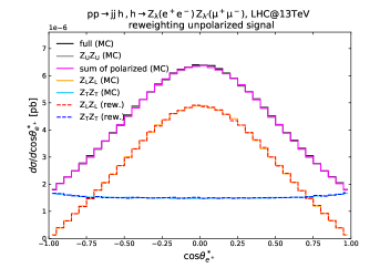
(a) $\cos\theta^{*}_{\text{e}^{+}}$

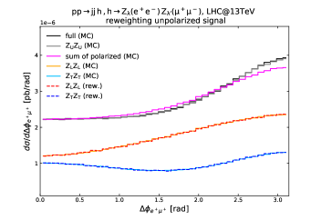
(b) $\Delta\phi_{\text{e}^{+}\mu^{+}}$

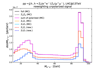
(c) $M_{\text{e}^{+}\text{e}^{-}}$

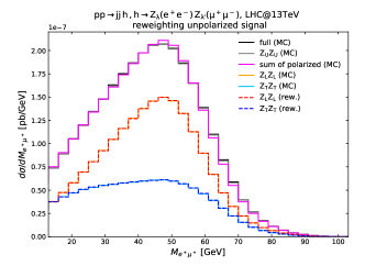
(d) $M_{\text{e}^{+}\mu^{+}}$

Figure 2: Differential cross-sections for VBF Higgs production at the LHC@13TeV: cosine of the positron decay angle in the corresponding Z boson rest frame (a), azimuthal difference (in the Higgs rest frame) between the positron and the antimuon (b), invariant mass of the positron-electron pair (c) and of the positron-antimuon pair (d). Comparison between the Monte Carlo polarized distributions (solid curves, label: MC) and the results of the matrix-element reweighting of the unpolarized-signal distribution (dashed curves, label: rew.). The LEP setup described in Sect. 4 is understood.

5 Validation of the method

In order to validate the matrix-element-reweighting method (MERM), we first compare the polarized cross sections computed with the MERM with those extracted from Phantom in VBF. In the first case, we reweight each unpolarized event as described in Sect. 2. In the second case, we use the approach of polarized amplitudes that has been already applied to VBS and di-boson production Ballestrero:2017bxn ; Ballestrero:2019qoy ; Denner:2020bcz ; Ballestrero:2020qgv ; Denner:2020eck . Differently from previous studies in VBS Ballestrero:2017bxn ; Ballestrero:2019qoy ; Ballestrero:2020qgv , we do not apply any double-pole approximation (DPA), since it is not possible to project both bosons on their mass shell. The comparison has been performed both in the INC setup and in the LEP one, and the results are shown in Table 1.

In the absence of lepton cuts, polarized cross sections can also be extracted from unpolarized angular distributions of the charged leptons, via appropriate projections onto Legendre polynomials Ballestrero:2017bxn . The corresponding results are presented in the third column of the INC section of Table 1. They agree with those computed by other means at the sub-percent level. In the LEP setup the cross sections computed with the MERM and those obtained from polarized amplitudes are in excellent agreement. This check ensures that separating polarizations of off-shell Z bosons from Higgs decay is well defined.

The reweighting method works very well also at the differential level, as can be appreciated in Fig. 2, where we consider four kinematic variables, in the LEP setup. The polarized distributions are perfectly reproduced by the reweighting both for the decay angle $\theta^{*}_{\text{e}^{+}}$ [Fig. 2(a)] that appears in Eqs. 2–2, and for the azimuthal difference $\Delta\phi_{\text{e}^{+}\mu^{+}}$ computed in the Higgs rest frame [Fig. 2(b)] with the z-axis defined by the Higgs direction of flight in the laboratory. Notice that this angular separation does not coincide with $\Delta\phi^{*}_{\text{e}^{+}\mu^{+}}$ in Eqs. 2–2, where the z-axis is defined by the Z boson direction of flight. The invariant-mass variables considered in Figs. 2(c)–2(d) are also perfectly described by the reweighting procedure. We stress that the impressive agreement is motivated by the fact that the reweighting factors of Eq. 11 are fully-differential. Therefore not only the variables appearing in the amplitude parametrization of Eq. 1, but any variable depending on the lepton momenta is well modelled, independently of the selection cuts that are applied.

We have successfully validated the method also for other observables, giving us confidence that the matrix-element reweighting procedure furnishes a useful tool to generate polarized observables from unpolarized ones.

6 Results

In this section we only consider the LEP setup defined in Sect. 4.

mode	GGF	VBF
unp.	6.988(5)$\cdot 10^{-6}\,$pb	8.566(5)$\cdot 10^{-6}\,$pb
LL	63.60%	64.26%
TT	36.35%	35.67%
interf.	0.05%	0.07%

Table 2: Total cross-sections and polarization fractions in the LEP setup. Numerical errors for the unpolarized signals are shown in parentheses.

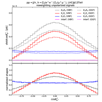
(a) $\cos\theta^{*}_{\text{e}^{+}}$

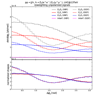
(b) $\Delta\phi_{\rm jj}$

Figure 3: Distributions for Higgs production in GGF (dashed curves) and VBF (solid curves) at the LHC@13TeV: cosine of the positron decay angle in the corresponding Z boson rest frame (a) and azimuthal difference between the two jets (b). Polarized VBF (GGF) curves are obtained via the matrix-element reweighting of the unpolarized VBF (GGF) distribution. Top panel: differential cross-sections. Bottom panel: normalized distributions (unit integral). The LEP setup described in Sect. 4 is understood.

Before starting the discussion on the VBF and GGF signals, it is worth commenting on the impact of some irreducible EW and QCD backgrounds. The evaluation of such backgrounds to the Higgs signal is in fact an important step in any polarization study. We have computed with Phantom the full process

$$\text{p}\,\text{p}\rightarrow\text{j}\,\text{j}\,\text{e}^{+}\text{e}^{-}\mu^{+}\mu^{-}\,,$$ (15)

which, at LO order $[\mathcal{O}(\alpha^{6})]$, receives contributions from several diagram topologies in which no $s$-channel Higgs propagator is present. However, the tight but realistic cut on the four-lepton invariant mass ($|M_{4\ell}-M_{\rm h}|<5\,\text{GeV}$), introduced in sec4, suppresses these non-signal contributions. The contribution from Higgs-strahlung is suppressed by the large jet-pair invariant-mass cut. The impact of all non-signal contributions on the total cross-section is below 0.5%.

The fiducial cross-section of the QCD background, computed at LO $[\mathcal{O}(\alpha_{\text{s}}^{2}\alpha^{4})]$ is 2.6% of the VBF signal. The signal cross-sections in GGF and VBF are shown in Table 2. The two LO cross-sections are of the same size. Given the very low statistics of the process it is essential to sum over them, provided that they show the same polarization structure. The sizable scale uncertainties that characterize the GGF channel [$6.988(5)^{+37.7\%}_{-25.4\%}\cdot 10^{-6}$ pb] make it important, in the lights of a realistic analysis, to include higher-order QCD corrections. The LO scale uncertainties in VBF production are much smaller [$8.566(5)^{+3.9\%}_{-3.8\%}\cdot 10^{-6}$ pb] and the NLO QCD corrections are expected to reduce them further. As already pointed out, the MERM applies, in the case of a Higgs-boson decay to four leptons, in exactly the same way whether radiative QCD corrections are included or not.

Table 2 shows that the polarization fractions (polarized cross-sections over the unpolarized one) amount to 65% for the longitudinal mode, 35% for the transverse one. These fractions are almost the same for the two signals, showing that in the SM the polarization content only depends on the decay of the Higgs, and not on its production mechanism. The small differences in the fractions can be traced back to the slightly different kinematics for the two signals, which implies different effects of the selection cuts. The interferences are very small, in spite of quite tight lepton cuts.

The results of Table 2 are not directly related to the SM Higgs coupling to vector bosons ($g_{\rm{\scalebox{0.6}{\rm hVV}}}$), which is independent of the polarization mode of the weak bosons. Therefore, a modification of $g_{\rm{\scalebox{0.6}{\rm hVV}}}$ due to new-physics effects would result in a enhanced (or diminished) cross-section at the unpolarized level, but one would not expect a strong modification of the relative weight of the longitudinal and the transverse mode. However, as shown in ref. Brehmer:2014pka , if a new-physics model allows for different Higgs couplings to longitudinal and transverse vector bosons, the effect on the polarization fractions would be relevant. In addition, since the GGF cross-section depends on $g_{\rm{\scalebox{0.6}{\rm hZZ}}}^{2}$, while the VBF one depends either on $g_{\rm{\scalebox{0.6}{\rm hZZ}}}^{4}$ or on $g_{\rm{\scalebox{0.6}{\rm hZZ}}}^{2}\,g_{\rm{\scalebox{0.6}{\rm hWW}}}^{2}$, polarization-dependent Higgs couplings to weak bosons could imply sizeable differences in the polarization structure of the GGF and the VBF signals. Therefore, a good understanding of both signals within the SM is the first step towards the search of beyond-SM effects via the polarization of weak-bosons.

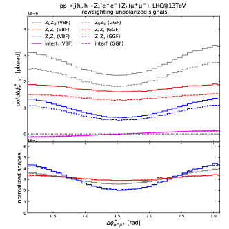
(a) $\Delta\phi^{*}_{\text{e}^{+}\mu^{+}}$

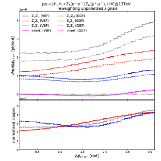
(b) $\Delta\phi_{\text{e}^{+}\mu^{+}}$

Figure 4: Distributions for Higgs production in GGF (dashed curves) and VBF (solid curves) at the LHC@13TeV: difference between the azimuthal decay angles of the positron and of the antimuon, computed in the corresponding Z-boson rest frame, starting from the Higgs-boson rest frame (a), azimuthal difference (in the Higgs rest frame) between the positron and the antimuon (b). Same structure as Fig. 3.

The integrated results are not enough to fully characterize the polarization structure in the Higgs-boson decay. The study of differential distributions is essential to identify LHC observables that are capable of discriminating among polarization states. Furthermore, the interference terms could give noticeable shape distortions, in spite of an integrated contribution which is close to zero.

In Figs. 3–5 we compare the distributions for different polarization states, separating the GGF and VBF production mechanisms. We present the results in terms of differential cross-sections (upper panels) and normalized shapes (lower panels).

In Fig. 3(a) we consider the cosine of the positron decay angle $\theta^{*}_{\text{e}^{+}}$ in the corresponding Z-boson rest frame, that is directly related to the polarization mode of the weak boson (see Eq. 1). This angular variable can be directly reconstructed at the LHC, thanks to the final state with four charged leptons. The VBF and GGF distributions have the same shape, both in the LL and in the TT component. The interferences play a negligible role for this distribution, as at the integrated level. The symmetric LL shape features a maximum at $\cos\theta^{*}_{\text{e}^{+}}=0$ and a minimum in the (anti)collinear regime, similar to the corresponding distribution in the INC setup ($d\sigma/d\cos\theta^{*}_{\text{e}^{+}}\propto f_{{\mathrm{L}}{\mathrm{L}}}\,(1-\cos^{2}\theta^{*}_{\text{e}^{+}})$). The TT distributions has constant convexity which is very close to zero, but with opposite sign w.r.t. the LL one. The noticeable difference in shape between the LL and the TT distributions makes this variable well suited for polarization discrimination.

In Fig. 3(b) we consider the azimuthal difference between the two tagging jets, computed in the laboratory frame. The GGF distribution shape is sizeably different from the VBF one, as expected from the different kinematics of the forward-backward jets in the two signals. In fact, this variable has been used to discriminate the GGF signal from its largest EW and QCD backgrounds in the $\rm h\rightarrow\text{W}\text{W}^{*}$ decay channel Klamke:2007cu . The LL and TT distributions in a given signal do not show relevant differences, as the kinematics of the decay leptons is just mildly affected by the different kinematics of the production part of the amplitudes. This azimuthal difference can be useful for polarization measurements only in combination with other variables that discriminate among polarization modes, and if it is needed to separate different signal processes.

In Fig. 4 we consider two azimuthal-difference variables that concern the charged-lepton kinematics.

The difference between the two azimuthal decay angles of the positively-charged leptons $\Delta\phi^{*}_{\text{e}^{+}\mu^{+}}$ is considered in Fig. 4(a). This variable appears in the squared-amplitude parametrization of Eq. 1, and gives a modulation to the interferences terms of Eqs. 2-2. In the INC setup the LL distribution is flat, while the TT one it is dominated by a $\cos(2\Delta\phi^{*}_{\text{e}^{+}\mu^{+}})$ functional dependence, since the interference between left and right modes is included in the cross-section Maina:2020rgd . In the LEP setup, the behaviour of the TT distribution is quite similar to the one in the INC setup, while the LL shape is no more flat.

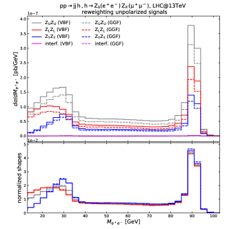
(a) $M_{\text{e}^{+}\text{e}^{-}}$

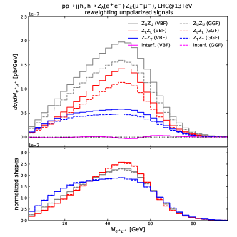
(b) $M_{\text{e}^{+}\mu^{+}}$

Figure 5: Distributions for Higgs production in GGF (dashed curves) and VBF (solid curves) at the LHC@13TeV: invariant mass of the positron-electron pair (a) and of the positron-antimuon pair (b). Same structure as Fig. 3.

The non-symmetric character of the unpolarized distributions is due to the longitudinal-transverse interferences that are negative for $\Delta\phi^{*}_{\text{e}^{+}\mu^{+}}<\pi/2$, positive otherwise. This effect (at most of 2%) reflects, even in the presence of lepton cuts, the $\cos(\Delta\phi^{*}_{\text{e}^{+}\mu^{+}})$ functional dependence of the interference terms of Eqs. 2-2. The GGF and VBF signals show exactly the same behaviour in all polarized contributions and interference terms. The $\Delta\phi^{*}_{\text{e}^{+}\mu^{+}}$ variable can be easily reconstructed at the LHC, with the considered final state, in the same fashion as $\cos\theta^{*}_{\text{e}^{+}}$.

In Fig. 4(b) we consider the azimuthal difference $\Delta\phi_{\text{e}^{+}\mu^{+}}$ between the positron and the antimuon computed in the Higgs-boson rest frame. This angular variable is related to $\Delta\phi^{*}_{\text{e}^{+}\mu^{+}}$, with the difference that $\Delta\phi_{\text{e}^{+}\mu^{+}}$ does not depend on angles computed in the Z-boson rest frame, but only on the kinematics of the four leptons in the Higgs-boson rest frame. The shapes of the polarized distributions is markedly different from those for $\Delta\phi^{*}_{\text{e}^{+}\mu^{+}}$. The interferences are very small and negative for $\Delta\phi_{\text{e}^{+}\mu^{+}}<3\pi/4$, positive and slightly larger in size for $\Delta\phi_{\text{e}^{+}\mu^{+}}>3\pi/4$. Also this variable enables a clear discrimination between the LL and TT modes. The LL shape is monotonically increasing from 0 to $\pi$, while the TT one has an absolute minimum at $\pi/2$, an absolute maximum at $\pi$ and another maximum at around 0. The impressive similarity of the SM polarized shapes for the GGF and VBF signals confirms that, if the focus is put on angular variables describing the Higgs-boson decay, it is safe to sum over production mechanisms.

As pointed out in ref. Maina:2020rgd , not only angular variables but also invariant-mass observables are suitable for polarization discrimination. In Fig. 5 we consider the invariant mass of the $\text{e}^{+}\text{e}^{-}$ and $\text{e}^{+}\mu^{+}$ pairs.

In the first case (Fig. 5(a)), the reconstructed Z-boson mass is peaked below $40\,\text{GeV}$ and at the pole mass, as at the Higgs resonance one Z is typically on-shell while the other is far off-shell. Interferences are almost negligible for this observable. The difference between the LL and the TT normalized shapes concerns only the off-shell region below $40\,\text{GeV}$: the longitudinal curve peaks between 20 and 25 GeV, while the transverse one has a narrower peak around 30 GeV. The GGF and VBF curves for a definite polarization state are almost identical, apart from mild differences in the TT curve around its two peaks.

The invariant mass of the two positively-charged leptons is shown in Fig. 5(b). The GGF and VBF signals behave in the same way, as for most of the other analyzed observables, giving distribution shapes that are almost independent of the production mode. The unpolarized and polarized distributions feature a maximum around $M_{\text{Z}}/2$, but the LL shape is narrower than the TT one, making this variable quite suitable for polarization discrimination. The polarization fractions (both for GGF and for VBF) show that the transverse mode gives a larger cross-sections than the longitudinal in the soft region ($M_{\text{e}^{+}\mu^{+}}<20\,\text{GeV}$), while the LL mode is larger in the rest of the spectrum. The interference pattern is slightly more evident than for $M_{\text{e}^{+}\text{e}^{-}}$. Its size is at most 2% of the total at moderate masses ($M_{\text{e}^{+}\mu^{+}}\approx 70\,\text{GeV}$). Comparing Fig. 5(b) with Fig. 9 in ref. Maina:2020rgd one notices that different selection cuts can produce significant distortions in the observed distributions.

As a last comment, we note that in the SM not only the polarized shapes but also the relative fraction of longitudinal and transverse modes are almost independent of the production channel. This results in unpolarized distributions shapes (gray curves in bottom panels of Figs. 3-5) that are also independent of the production channel.

7 Conclusions

In this paper we have studied the polarization of Z bosons decaying from a Higgs boson produced in association with two jets, in a vector-boson-fusion kinematic regime.

We have proved that, thanks to the simple analytic structure of the Higgs-decay Standard-Model amplitude, it is possible to avoid generating separately polarized event samples by simply reweighting unpolarized events with fully-differential weights.

We have considered the two main channels that give contribution to Higgs+2j production, namely gluon-gluon fusion and vector-boson fusion. The polarized signals show the same behaviour in the two channels, both at the level of polarization fractions, and at the level of the shape of polarized distributions. This allows to sum over production channels. This holds for a SM measurement, and for modelling the background for the search of beyond-the-Standard-Model effects.

The possibility of extending this work to higher-orders in perturbation theory is also addressed. The usage of a single-pole approximation enables the description of the Higgs decay to polarized bosons in the presence of EW radiative corrections.

The results presented in this paper provide general techniques to study polarizations of vector bosons from the decay of a scalar Higgs boson produced in any channel at hadron colliders. The extension of such methods to an effective-field-theory framework allows for a model-independent assessment of the polarization structure at the Higgs resonance in the presence of new-physics effects.

References

- (1) S. Chatrchyan, et al., Observation of a new boson at a mass of 125 GeV with the CMS experiment at the LHC, Phys. Lett. B716 (2012) 30–61. arXiv:1207.7235, doi:10.1016/j.physletb.2012.08.021.
- (2) G. Aad, et al., Observation of a new particle in the search for the Standard Model Higgs boson with the ATLAS detector at the LHC, Phys. Lett. B716 (2012) 1–29. arXiv:1207.7214, doi:10.1016/j.physletb.2012.08.020.
- (3) D. A. Dicus, V. S. Mathur, Upper bounds on the values of masses in unified gauge theories, Phys. Rev. D 7 (1973) 3111–3114. doi:10.1103/PhysRevD.7.3111.
- (4) C. H. Llewellyn Smith, High-Energy Behavior and Gauge Symmetry, Phys. Lett. B 46 (1973) 233–236. doi:10.1016/0370-2693(73)90692-8.
- (5) M. J. G. Veltman, Second Threshold in Weak Interactions, Acta Phys. Polon. B 8 (1977) 475.
- (6) J. Brehmer, J. Jaeckel, T. Plehn, Polarized WW Scattering on the Higgs Pole, Phys. Rev. D 90 (5) (2014) 054023. arXiv:1404.5951, doi:10.1103/PhysRevD.90.054023.
- (7) S. Chatrchyan, et al., Measurement of the Properties of a Higgs Boson in the Four-Lepton Final State, Phys. Rev. D 89 (9) (2014) 092007. arXiv:1312.5353, doi:10.1103/PhysRevD.89.092007.
- (8) G. Aad, et al., Measurements of Higgs boson production and couplings in the four-lepton channel in pp collisions at center-of-mass energies of 7 and 8 TeV with the ATLAS detector, Phys. Rev. D 91 (1) (2015) 012006. arXiv:1408.5191, doi:10.1103/PhysRevD.91.012006.
- (9) A. M. Sirunyan, et al., Measurements of properties of the Higgs boson decaying into the four-lepton final state in pp collisions at TeV, JHEP 11 (2017) 047. arXiv:1706.09936, doi:10.1007/JHEP11(2017)047.
- (10) V. Khachatryan, et al., Constraints on the Higgs boson width from off-shell production and decay to Z-boson pairs, Phys. Lett. B 736 (2014) 64–85. arXiv:1405.3455, doi:10.1016/j.physletb.2014.06.077.
- (11) V. Khachatryan, et al., Limits on the Higgs boson lifetime and width from its decay to four charged leptons, Phys. Rev. D 92 (7) (2015) 072010. arXiv:1507.06656, doi:10.1103/PhysRevD.92.072010.
- (12) A. M. Sirunyan, et al., Measurements of the Higgs boson width and anomalous couplings from on-shell and off-shell production in the four-lepton final state, Phys. Rev. D 99 (11) (2019) 112003. arXiv:1901.00174, doi:10.1103/PhysRevD.99.112003.
- (13) V. Khachatryan, et al., Constraints on the spin-parity and anomalous HVV couplings of the Higgs boson in proton collisions at 7 and 8 TeV, Phys. Rev. D 92 (1) (2015) 012004. arXiv:1411.3441, doi:10.1103/PhysRevD.92.012004.
- (14) M. Aaboud, et al., Measurement of the Higgs boson coupling properties in the decay channel at = 13 TeV with the ATLAS detector, JHEP 03 (2018) 095. arXiv:1712.02304, doi:10.1007/JHEP03(2018)095.
- (15) G. Aad, et al., Higgs boson production cross-section measurements and their EFT interpretation in the decay channel at 13 TeV with the ATLAS detector, Eur. Phys. J. C 80 (10) (2020) 957, [Erratum: Eur.Phys.J.C 81, 29 (2021)]. arXiv:2004.03447, doi:10.1140/epjc/s10052-020-8227-9.
- (16) G. Aad, et al., Fiducial and differential cross sections of Higgs boson production measured in the four-lepton decay channel in collisions at =8 TeV with the ATLAS detector, Phys. Lett. B 738 (2014) 234–253. arXiv:1408.3226, doi:10.1016/j.physletb.2014.09.054.
- (17) V. Khachatryan, et al., Measurement of differential and integrated fiducial cross sections for Higgs boson production in the four-lepton decay channel in pp collisions at and 8 TeV, JHEP 04 (2016) 005. arXiv:1512.08377, doi:10.1007/JHEP04(2016)005.
- (18) M. Aaboud, et al., Measurement of inclusive and differential cross sections in the decay channel in collisions at TeV with the ATLAS detector, JHEP 10 (2017) 132. arXiv:1708.02810, doi:10.1007/JHEP10(2017)132.
- (19) G. Aad, et al., Measurements of the Higgs boson inclusive and differential fiducial cross sections in the 4 decay channel at = 13 TeV, Eur. Phys. J. C 80 (10) (2020) 942. arXiv:2004.03969, doi:10.1140/epjc/s10052-020-8223-0.
- (20) A. M. Sirunyan, et al., Measurements of production cross sections of the Higgs boson in the four-lepton final state in proton-proton collisions at 13 TeV, (3 2021). arXiv:2103.04956.
- (21) A. M. Sirunyan, et al., Constraints on anomalous Higgs boson couplings using production and decay information in the four-lepton final state, Phys. Lett. B 775 (2017) 1–24. arXiv:1707.00541, doi:10.1016/j.physletb.2017.10.021.
- (22) M. Aaboud, et al., Constraints on off-shell Higgs boson production and the Higgs boson total width in and final states with the ATLAS detector, Phys. Lett. B 786 (2018) 223–244. arXiv:1808.01191, doi:10.1016/j.physletb.2018.09.048.
- (23) A. M. Sirunyan, et al., Constraints on anomalous Higgs boson couplings to vector bosons and fermions in its production and decay using the four-lepton final state (4 2021). arXiv:2104.12152.
- (24) A. Bredenstein, A. Denner, S. Dittmaier, M. M. Weber, Precise predictions for the Higgs-boson decay H WW/ZZ 4 leptons, Phys. Rev. D 74 (2006) 013004. arXiv:hep-ph/0604011, doi:10.1103/PhysRevD.74.013004.
- (25) S. Boselli, C. M. Carloni Calame, G. Montagna, O. Nicrosini, F. Piccinini, Higgs boson decay into four leptons at NLOPS electroweak accuracy, JHEP 06 (2015) 023. arXiv:1503.07394, doi:10.1007/JHEP06(2015)023.
- (26) L. Altenkamp, M. Boggia, S. Dittmaier, Precision calculations for fermions in a Singlet Extension of the Standard Model with Prophecy4f, JHEP 04 (2018) 062. arXiv:1801.07291, doi:10.1007/JHEP04(2018)062.
- (27) L. Altenkamp, M. Boggia, S. Dittmaier, H. Rzehak, Electroweak corrections in the Two-Higgs-Doublet Model and Singlet Extension of the Standard Model, PoS LL2018 (2018) 011. arXiv:1807.05876, doi:10.22323/1.303.0011.
- (28) S. Kanemura, M. Kikuchi, K. Mawatari, K. Sakurai, K. Yagyu, Full next-to-leading-order calculations of Higgs boson decay rates in models with non-minimal scalar sectors, Nucl. Phys. B 949 (2019) 114791. arXiv:1906.10070, doi:10.1016/j.nuclphysb.2019.114791.
- (29) P. Artoisenet, et al., A framework for Higgs characterisation, JHEP 11 (2013) 043. arXiv:1306.6464, doi:10.1007/JHEP11(2013)043.
- (30) S. Boselli, C. M. Carloni Calame, G. Montagna, O. Nicrosini, F. Piccinini, A. Shivaji, Higgs decay into four charged leptons in the presence of dimension-six operators, JHEP 01 (2018) 096. arXiv:1703.06667, doi:10.1007/JHEP01(2018)096.
- (31) I. Brivio, T. Corbett, M. Trott, The Higgs width in the SMEFT, JHEP 10 (2019) 056. arXiv:1906.06949, doi:10.1007/JHEP10(2019)056.
- (32) A. Soni, R. M. Xu, Probing CP violation via Higgs decays to four leptons, Phys. Rev. D 48 (1993) 5259–5263. arXiv:hep-ph/9301225, doi:10.1103/PhysRevD.48.5259.
- (33) D. Chang, W.-Y. Keung, I. Phillips, CP odd correlation in the decay of neutral Higgs boson into Z Z, W+ W-, or t anti-t, Phys. Rev. D 48 (1993) 3225–3234. arXiv:hep-ph/9303226, doi:10.1103/PhysRevD.48.3225.
- (34) A. Skjold, P. Osland, Angular and energy correlations in Higgs decay, Phys. Lett. B 311 (1993) 261–265. arXiv:hep-ph/9303294, doi:10.1016/0370-2693(93)90565-Y.
- (35) T. Arens, L. M. Sehgal, Energy spectra and energy correlations in the decay H Z Z mu+ mu- mu+ mu-, Z. Phys. C 66 (1995) 89–94. arXiv:hep-ph/9409396, doi:10.1007/BF01496583.
- (36) C. P. Buszello, I. Fleck, P. Marquard, J. J. van der Bij, Prospective analysis of spin- and CP-sensitive variables in H Z Z l(1)+ l(1)- l(2)+ l(2)- at the LHC, Eur. Phys. J. C 32 (2004) 209–219. arXiv:hep-ph/0212396, doi:10.1140/epjc/s2003-01392-0.
- (37) S. Y. Choi, D. J. Miller, M. M. Muhlleitner, P. M. Zerwas, Identifying the Higgs spin and parity in decays to Z pairs, Phys. Lett. B 553 (2003) 61–71. arXiv:hep-ph/0210077, doi:10.1016/S0370-2693(02)03191-X.
- (38) K. Hagiwara, Q. Li, K. Mawatari, Jet angular correlation in vector-boson fusion processes at hadron colliders, JHEP 07 (2009) 101. arXiv:0905.4314, doi:10.1088/1126-6708/2009/07/101.
- (39) Y. Gao, A. V. Gritsan, Z. Guo, K. Melnikov, M. Schulze, N. V. Tran, Spin Determination of Single-Produced Resonances at Hadron Colliders, Phys. Rev. D 81 (2010) 075022. arXiv:1001.3396, doi:10.1103/PhysRevD.81.075022.
- (40) S. Bolognesi, Y. Gao, A. V. Gritsan, K. Melnikov, M. Schulze, N. V. Tran, A. Whitbeck, On the spin and parity of a single-produced resonance at the LHC, Phys. Rev. D 86 (2012) 095031. arXiv:1208.4018, doi:10.1103/PhysRevD.86.095031.
- (41) S. Berge, S. Groote, J. G. Körner, L. Kaldamäe, Lepton-mass effects in the decays and , Phys. Rev. D 92 (3) (2015) 033001. arXiv:1505.06568, doi:10.1103/PhysRevD.92.033001.
- (42) V. Del Duca, W. Kilgore, C. Oleari, C. Schmidt, D. Zeppenfeld, Higgs + 2 jets via gluon fusion, Phys. Rev. Lett. 87 (2001) 122001. arXiv:hep-ph/0105129, doi:10.1103/PhysRevLett.87.122001.
- (43) V. Del Duca, W. Kilgore, C. Oleari, C. Schmidt, D. Zeppenfeld, Gluon fusion contributions to H + 2 jet production, Nucl. Phys. B 616 (2001) 367–399. arXiv:hep-ph/0108030, doi:10.1016/S0550-3213(01)00446-1.
- (44) N. Greiner, S. Höche, G. Luisoni, M. Schönherr, J.-C. Winter, Full mass dependence in Higgs boson production in association with jets at the LHC and FCC, JHEP 01 (2017) 091. arXiv:1608.01195, doi:10.1007/JHEP01(2017)091.
- (45) G. Cullen, H. van Deurzen, N. Greiner, G. Luisoni, P. Mastrolia, E. Mirabella, G. Ossola, T. Peraro, F. Tramontano, Next-to-Leading-Order QCD Corrections to Higgs Boson Production Plus Three Jets in Gluon Fusion, Phys. Rev. Lett. 111 (13) (2013) 131801. arXiv:1307.4737, doi:10.1103/PhysRevLett.111.131801.
- (46) J. R. Andersen, J. D. Cockburn, M. Heil, A. Maier, J. M. Smillie, Finite Quark-Mass Effects in Higgs Boson Production with Dijets at Large Energies, JHEP 04 (2019) 127. arXiv:1812.08072, doi:10.1007/JHEP04(2019)127.
- (47) M. Ciccolini, A. Denner, S. Dittmaier, Strong and electroweak corrections to the production of Higgs + 2jets via weak interactions at the LHC, Phys. Rev. Lett. 99 (2007) 161803. arXiv:0707.0381, doi:10.1103/PhysRevLett.99.161803.
- (48) F. A. Dreyer, A. Karlberg, Vector-Boson Fusion Higgs Production at Three Loops in QCD, Phys. Rev. Lett. 117 (7) (2016) 072001. arXiv:1606.00840, doi:10.1103/PhysRevLett.117.072001.
- (49) T. Han, G. Valencia, S. Willenbrock, Structure function approach to vector boson scattering in p p collisions, Phys. Rev. Lett. 69 (1992) 3274–3277. arXiv:hep-ph/9206246, doi:10.1103/PhysRevLett.69.3274.
- (50) M. Buschmann, C. Englert, D. Goncalves, T. Plehn, M. Spannowsky, Resolving the Higgs-Gluon Coupling with Jets, Phys. Rev. D 90 (1) (2014) 013010. arXiv:1405.7651, doi:10.1103/PhysRevD.90.013010.
- (51) M. Buschmann, D. Goncalves, S. Kuttimalai, M. Schonherr, F. Krauss, T. Plehn, Mass Effects in the Higgs-Gluon Coupling: Boosted vs Off-Shell Production, JHEP 02 (2015) 038. arXiv:1410.5806, doi:10.1007/JHEP02(2015)038.
- (52) J. M. Campbell, R. K. Ellis, R. Frederix, P. Nason, C. Oleari, C. Williams, NLO Higgs Boson Production Plus One and Two Jets Using the POWHEG BOX, MadGraph4 and MCFM, JHEP 07 (2012) 092. arXiv:1202.5475, doi:10.1007/JHEP07(2012)092.
- (53) J. R. Andersen, T. Binoth, G. Heinrich, J. M. Smillie, Loop induced interference effects in Higgs Boson plus two jet production at the LHC, JHEP 02 (2008) 057. arXiv:0709.3513, doi:10.1088/1126-6708/2008/02/057.
- (54) S. Chatrchyan, et al., Measurement of the Polarization of W Bosons with Large Transverse Momenta in W+Jets Events at the LHC, Phys. Rev. Lett. 107 (2011) 021802. arXiv:1104.3829, doi:10.1103/PhysRevLett.107.021802.
- (55) G. Aad, et al., Measurement of the polarisation of bosons produced with large transverse momentum in collisions at 7 TeV with the ATLAS experiment, Eur. Phys. J. C72 (2012) 2001. arXiv:1203.2165, doi:10.1140/epjc/s10052-012-2001-6.
- (56) V. Khachatryan, et al., Angular coefficients of Z bosons produced in pp collisions at 8 TeV and decaying to as a function of transverse momentum and rapidity, Phys. Lett. B750 (2015) 154–175. arXiv:1504.03512, doi:10.1016/j.physletb.2015.08.061.
- (57) G. Aad, et al., Measurement of the angular coefficients in -boson events using electron and muon pairs from data taken at 8 TeV with th e ATLAS detector, JHEP 08 (2016) 159. arXiv:1606.00689, doi:10.1007/JHEP08(2016)159.
- (58) M. Aaboud, et al., Measurement of production cross sections and gauge boson polarisation in collisions at TeV with the ATLA S detector, Eur. Phys. J. C 79 (6) (2019) 535. arXiv:1902.05759, doi:10.1140/epjc/s10052-019-7027-6.
- (59) A. M. Sirunyan, et al., Measurements of production cross sections of polarized same-sign W boson pairs in association with two jets in proton-proton collisions at 13 TeV, Phys. Lett. B 812 (2021) 136018. arXiv:2009.09429, doi:10.1016/j.physletb.2020.136018.
- (60) M. Aaboud, et al., Measurement of the boson polarisation in events from collisions at 8 TeV in the lepton+jets channel with ATLAS (2016). arXiv:1612.02577.
- (61) V. Khachatryan, et al., Measurement of the W boson helicity fractions in the decays of top quark pairs to lepton jets final states produced in pp collisions at 8 TeV, Phys. Lett. B762 (2016) 512–534. arXiv:1605.09047, doi:10.1016/j.physletb.2016.10.007.
- (62) G. Aad, et al., Combination of the W boson polarization measurements in top quark decays using ATLAS and CMS data at 8 TeV (5 2020). arXiv:2005.03799.
- (63) M. Aaboud, et al., Measurements of gluon-gluon fusion and vector-boson fusion Higgs boson production cross-sections in the decay channel in collisions at TeV with the ATLAS detector, Phys. Lett. B 789 (2019) 508–529. arXiv:1808.09054, doi:10.1016/j.physletb.2018.11.064.
- (64) L. S. Bruni, Polarized on Higgs? Measurement of the Higgs couplings to polarized vector bosons, Ph.D. thesis, Twente U., Enschede (2019). doi:10.3990/1.9789036547215.
-
(65)
Vector Boson Scattering prospective
studies in the ZZ fully leptonic decay channel for the High-Luminosity and
High-Energy LHC upgrades, Tech. Rep. CMS-PAS-FTR-18-014, CERN, Geneva
(2018).
URL https://cds.cern.ch/record/2650915 - (66) P. Azzi, et al., Report from Working Group 1: Standard Model Physics at the HL-LHC and HE-LHC, Vol. 7, 2019, pp. 1–220. arXiv:1902.04070, doi:10.23731/CYRM-2019-007.1.
- (67) Z. Bern, et al., Left-Handed W Bosons at the LHC, Phys. Rev. D84 (2011) 034008. arXiv:1103.5445, doi:10.1103/PhysRevD.84.034008.
- (68) W. J. Stirling, E. Vryonidou, Electroweak gauge boson polarisation at the LHC, JHEP 07 (2012) 124. arXiv:1204.6427, doi:10.1007/JHEP07(2012)124.
- (69) A. Belyaev, D. Ross, What Does the CMS Measurement of W-polarization Tell Us about the Underlying Theory of the Coupling of W-Bosons to Matter?, JHEP 08 (2013) 120. arXiv:1303.3297, doi:10.1007/JHEP08(2013)120.
- (70) A. Ballestrero, E. Maina, G. Pelliccioli, boson polarization in vector boson scattering at the LHC, JHEP 03 (2018) 170. arXiv:1710.09339, doi:10.1007/JHEP03(2018)170.
- (71) A. Ballestrero, E. Maina, G. Pelliccioli, Polarized vector boson scattering in the fully leptonic WZ and ZZ channels at the LHC, JHEP 09 (2019) 087. arXiv:1907.04722, doi:10.1007/JHEP09(2019)087.
- (72) A. Ballestrero, E. Maina, G. Pelliccioli, Different polarization definitions in same-sign scattering at the LHC, Phys. Lett. B 811 (2020) 135856. arXiv:2007.07133, doi:10.1016/j.physletb.2020.135856.
- (73) A. Denner, G. Pelliccioli, Polarized electroweak bosons in production at the LHC including NLO QCD effects, JHEP 09 (2020) 164. arXiv:2006.14867, doi:10.1007/JHEP09(2020)164.
- (74) A. Denner, G. Pelliccioli, NLO QCD predictions for doubly-polarized WZ production at the LHC, Phys. Lett. B 814 (2021) 136107. arXiv:2010.07149, doi:10.1016/j.physletb.2021.136107.
- (75) J. Baglio, N. Le Duc, Fiducial polarization observables in hadronic WZ production: A next-to-leading order QCD+EW study, JHEP 04 (2019) 065. arXiv:1810.11034, doi:10.1007/JHEP04(2019)065.
- (76) J. Baglio, L. D. Ninh, Polarization observables in WZ production at the 13 TeV LHC: Inclusive case, Commun. Phys. 30 (1) (2020) 35–47. arXiv:1910.13746, doi:10.15625/0868-3166/30/1/14461.
- (77) D. Buarque Franzosi, O. Mattelaer, R. Ruiz, S. Shil, Automated predictions from polarized matrix elements, JHEP 04 (2020) 082. arXiv:1912.01725, doi:10.1007/JHEP04(2020)082.
- (78) Q.-H. Cao, B. Yan, C. P. Yuan, Y. Zhang, Probing couplings using boson polarization in production at hadron colliders, Phys. Rev. D 102 (5) (2020) 055010. arXiv:2004.02031, doi:10.1103/PhysRevD.102.055010.
- (79) E. Maina, Vector boson polarizations in the decay of the Standard Model Higgs, , Phys. Lett. B 818 (2021) 136360. arXiv:2007.12080, doi:10.1016/j.physletb.2021.136360.
- (80) G. Klamke, D. Zeppenfeld, Higgs plus two jet production via gluon fusion as a signal at the CERN LHC, JHEP 04 (2007) 052. arXiv:hep-ph/0703202, doi:10.1088/1126-6708/2007/04/052.
- (81) J. R. Andersen, V. Del Duca, C. D. White, Higgs Boson Production in Association with Multiple Hard Jets, JHEP 02 (2009) 015. arXiv:0808.3696, doi:10.1088/1126-6708/2009/02/015.
- (82) J. R. Andersen, C. Englert, M. Spannowsky, Extracting precise Higgs couplings by using the matrix element method, Phys. Rev. D 87 (1) (2013) 015019. arXiv:1211.3011, doi:10.1103/PhysRevD.87.015019.
- (83) F. Demartin, F. Maltoni, K. Mawatari, B. Page, M. Zaro, Higgs characterisation at NLO in QCD: CP properties of the top-quark Yukawa interaction, Eur. Phys. J. C 74 (9) (2014) 3065. arXiv:1407.5089, doi:10.1140/epjc/s10052-014-3065-2.
- (84) A. Denner, S. Dittmaier, M. Roth, D. Wackeroth, Electroweak radiative corrections to fermions in double pole approximation: The RACOONWW approach, Nucl. Phys. B587 (2000) 67–117. arXiv:hep-ph/0006307, doi:10.1016/S0550-3213(00)00511-3.
- (85) A. Denner, S. Dittmaier, Electroweak Radiative Corrections for Collider Physics, Phys. Rept. 864 (2020) 1–163. arXiv:1912.06823, doi:10.1016/j.physrep.2020.04.001.
- (86) R. G. Stuart, Gauge invariance, analyticity and physical observables at the Z0 resonance, Phys. Lett. B 262 (1991) 113–119. doi:10.1016/0370-2693(91)90653-8.
- (87) A. Aeppli, G. J. van Oldenborgh, D. Wyler, Unstable particles in one loop calculations, Nucl. Phys. B 428 (1994) 126–146. arXiv:hep-ph/9312212, doi:10.1016/0550-3213(94)90195-3.
- (88) A. Denner, S. Dittmaier, M. Roth, Nonfactorizable photonic corrections to four fermions, Nucl. Phys. B 519 (1998) 39–84. arXiv:hep-ph/9710521, doi:10.1016/S0550-3213(98)00046-7.
- (89) S. Dittmaier, C. Schwan, Non-factorizable photonic corrections to resonant production and decay of many unstable particles, Eur. Phys. J. C 76 (3) (2016) 144. arXiv:1511.01698, doi:10.1140/epjc/s10052-016-3968-1.
- (90) R. D. Ball, et al., Parton distributions for the LHC Run II, JHEP 04 (2015) 040. arXiv:1410.8849, doi:10.1007/JHEP04(2015)040.
- (91) A. Buckley, J. Ferrando, S. Lloyd, K. Nordström, B. Page, M. Rüfenacht, M. Schönherr, G. Watt, LHAPDF6: parton density access in the LHC precision era, Eur. Phys. J. C 75 (2015) 132. arXiv:1412.7420, doi:10.1140/epjc/s10052-015-3318-8.
- (92) A. Denner, S. Dittmaier, M. Roth, L. H. Wieders, Electroweak corrections to charged-current fermion processes: Technical details and further results, Nucl. Phys. B724 (2005) 247–294, [Erratum: Nucl. Phys. B 854 (2012) 504]. arXiv:hep-ph/0505042, doi:10.1016/j.nuclphysb.2011.09.001,10.1016/j.nuclphysb.2005.06.033.
- (93) A. Denner, S. Dittmaier, The complex-mass scheme for perturbative calculations with unstable particles, Nucl. Phys. B Proc. Suppl. 160 (2006) 22–26. arXiv:hep-ph/0605312, doi:10.1016/j.nuclphysbps.2006.09.025.
- (94) M. Cacciari, F. A. Dreyer, A. Karlberg, G. P. Salam, G. Zanderighi, Fully Differential Vector-Boson-Fusion Higgs Production at Next-to-Next-to-Leading Order, Phys. Rev. Lett. 115 (8) (2015) 082002, [Erratum: Phys.Rev.Lett. 120, 139901 (2018)]. arXiv:1506.02660, doi:10.1103/PhysRevLett.115.082002.
- (95) A. Denner, R. Franken, M. Pellen, T. Schmidt, NLO QCD and EW corrections to vector-boson scattering into ZZ at the LHC, JHEP 11 (2020) 110. arXiv:2009.00411, doi:10.1007/JHEP11(2020)110.
- (96) G. Aad, et al., Measurements of differential cross-sections in four-lepton events in 13 TeV proton-proton collisions with the ATLAS detector, (3 2021). arXiv:2103.01918.
- (97) A. Ballestrero, A. Belhouari, G. Bevilacqua, V. Kashkan, E. Maina, PHANTOM: A Monte Carlo event generator for six parton final states at high energy colliders, Comput. Phys. Commun. 180 (2009) 401–417. arXiv:0801.3359, doi:10.1016/j.cpc.2008.10.005.
- (98) A. Ballestrero, E. Maina, Interference Effects in Higgs production through Vector Boson Fusion in the Standard Model and its Singlet Extension, JHEP 01 (2016) 045. arXiv:1506.02257, doi:10.1007/JHEP01(2016)045.
- (99) J. Alwall, R. Frederix, S. Frixione, V. Hirschi, F. Maltoni, O. Mattelaer, H. S. Shao, T. Stelzer, P. Torrielli, M. Zaro, The automated computation of tree-level and next-to-leading order differential cross sections, and their matching to parton shower simulations, JHEP 07 (2014) 079. arXiv:1405.0301, doi:10.1007/JHEP07(2014)079.