Full operator preconditioning and the accuracy of solving linear systems

Abstract

Unless special conditions apply, the attempt to solve ill-conditioned systems of linear equations with standard numerical methods leads to uncontrollably high numerical error. Often, such systems arise from the discretization of operator equations with a large number of discrete variables. In this paper we show that the accuracy can be improved significantly if the equation is transformed before discretization, a process we call full operator preconditioning (FOP). It bears many similarities with traditional preconditioning for iterative methods but, crucially, transformations are applied at the operator level. We show that while condition-number improvements from traditional preconditioning generally do not improve the accuracy of the solution, FOP can. A number of topics in numerical analysis can be interpreted as implicitly employing FOP; we highlight (i) Chebyshev interpolation in polynomial approximation, and (ii) Olver-Townsend’s spectral method, both of which produce solutions of dramatically improved accuracy over a naive problem formulation. In addition, we propose a FOP preconditioner based on integration for the solution of fourth-order differential equations with the finite-element method, showing the resulting linear system is well-conditioned regardless of the discretization size, and demonstrate its error-reduction capabilities on several examples. This work shows that FOP can improve accuracy beyond the standard limit for both direct and iterative methods.

1 Introduction

Ill-conditioned linear systems $\mathbf{Ax}=\mathbf{b}$ cannot be solved to high accuracy: even with a backward stable solution $\mathbf{\hat{x}}$ satisfying $(\mathbf{A}+\Delta\mathbf{A})\mathbf{\hat{x}}=\mathbf{b}$ with $\|\Delta\mathbf{A}\|_{2}=O(\epsilon\|\mathbf{A}\|_{2})$ where $\epsilon$ is on the order of machine precision, it is well known that we only have $\|\mathbf{\hat{x}}-\mathbf{x}\|_{2}/\|\mathbf{x}\|_{2}\lesssim\epsilon\kappa(\mathbf{A})$, where $\kappa(\mathbf{A})=\|\mathbf{A}\|_{2}\|\mathbf{A}^{-1}\|_{2}$ denotes the $2$-norm matrix condition number [31, § 1.6]. In other words, once the linear system has been set up, there is no way to reduce the numerical error, except by going to higher-precision arithmetic or employing a symbolic solver [22, § 7.3], [31, § 1.3].

In this paper, we present and discuss a method that attempts to circumvent this deadlock by taking the only possible route out: Reformulating the problem. The method is applicable to systems of linear equations arising from the discretization of an equation posed in continuous spaces, where the matrix of coefficients is the finite-dimensional representation of a linear operator. Here it is often the discretization size that determines the conditioning of the linear problem: the higher the number of rows and columns of the matrix, the worse its conditioning typically becomes, until one obtains garbage or even numerical blow-up [30].

Our approach is inspired by the preconditioning of linear systems used for the acceleration of iterative methods. It shares the goal of transforming the problem into one that is more easily solvable, and—often used as a historical explanation for the term “preconditioning” [47]—it usually aims at reducing the condition number. The crucial difference is the level of abstraction at which the transformation takes place: Whereas traditional preconditioning applies transformation matrices to the potentially ill-conditioned linear system after discretization has taken place, the presented method transforms the operator itself before discretization. We call our approach full operator preconditioning (FOP), emphasizing the structural similarities, but indicating that transformations take place on the operator level instead of the matrix level, and distinguishing it from what is conventionally called operator preconditioning or PDE-inspired preconditioning by other authors [3, 32, 35], which is a form of traditional preconditioning; see Section 2.4 for a discussion.

Traditional (matrix) preconditioning has the goal of speeding up an iterative method for solving linear systems by clustering the spectrum of the preconditioned matrix, so that a Krylov subspace method converges in a small number of iterations [47]. While reducing conditioning is sufficient in the symmetric case, it is neither sufficient nor necessary for fast convergence for general matrices [22, Chapter 3.2]. An underappreciated fact is that, unless special structure is present, matrix preconditioning does not improve the accuracy of the computed solution. FOP, by contrast, does.

To illustrate the idea of FOP, we give the following rough example: Let $\mathcal{L}$ be a linear differential operator and $u$ and $f$ functions such that

$$\mathcal{L}u=f.$$ (1.1)

Precise definitions are given in the next sections. This equation is normally tackled by choosing an appropriate discretization such as finite differences [33], finite elements [29] or spectral methods [21, 44], which represents the operator $\mathcal{L}$ as a square matrix $\mathbf{L}$. If $\mathbf{L}$ is highly ill-conditioned $\kappa(\mathbf{L})\geq\epsilon^{-1}$, then computed results could be useless even with an excellent (backward stable) method.

Now assume that there is a solution operator $\mathcal{R}$ inverting the differential operator $\mathcal{L}$ with appropriate boundary conditions. By applying $\mathcal{R}$ from the left, we transform equation (1.1) to

$$\mathcal{I}u=g,$$ (1.2)

with the identity operator $\mathcal{I}$ and right-hand side $g=\mathcal{R}f$. While the form of equation (1.2) may look tautologous with the trivial solution $u=g$, it was chosen intentionally to point out that it is amenable to the same discretization-plus-numerical-solver strategy as the original equation. But now the operator to be discretized is the identity instead of the differential operator $\mathcal{L}$. A reasonable discretization scheme then leads to well-conditioned matrices regardless of the the number of terms.

Equation (1.1) is a type of operator equation. These equations are all tackled in a similar fashion, and examples besides differential equations include integral equations and interpolation [40, Ch. 12]. All examples considered later in this paper arise from operator equations. For this reason, we dedicate the first part of Section 2 to introduce their discretization. We also discuss two types of error—numerical and discretization error—which are affected differently by changing the discretization. We then give our formal definition of FOP, highlighting the contrasts with the traditional notion of preconditioning. We then explain why FOP can help improve the accuracy in solving ill-conditioned linear systems while matrix preconditioning in general cannot, a fact that has been treated as a sidenote in the literature [22, § 7.3], and is—to our knowledge—first discussed here in full detail.

As we will see, FOP is already implicitly part of many methods of numerical analysis. In the following three sections, we demonstrate the power of the full-operator approach with three examples. We start by looking at the classical subject of polynomial interpolation of a univariate function. In Section 3.1, we formulate the task as the discretization of an operator equation involving the identity operator. We interpret changes between different bases of polynomials as FOP and show that such a change can lead to system-size-independent conditioning, completely removing numerical instabilities.

Section 4 continues with a discussion of spectral methods. We investigate a method by Olver and Townsend [39]: a change from Chebyshev to ultraspherical polynomials leads to a remarkable reduction of the condition number and accurate solution. This can be regarded as an application of FOP, however, it is not identified as such in the original paper.

In section 5, we turn to finite-element discretizations. Generalizing the observations in the previous sections, we design a FOP preconditioner for fourth-order differential equations in one dimension. It is based on the idea of solving the biharmonic equation algorithmically for the finite-element basis functions and, as we show in Section 5, it reduces the growth of the norm of associated matrices from $\mathcal{O}(n^{4})$ to $\mathcal{O}(1)$ while also guaranteeing their invertibility. Numerical examples illustrate that it allows reduction of the total error below the limit imposed by numerical error in the unpreconditioned system.

FOP is also related to the literature on integral equations. By recasting a problem (often differential equation) as an integral equation, the resulting conditioning of the linear system is often significantly better (e.g. [24, 25]), leading to more accurate solutions. This paper shows that a similar idea can be employed in a number of problems in numerical analysis.

We conclude the paper with a summary, an outlook onto potential topics of further research, and a statement about the implications of the topics discussed in this paper.

2 Mathematical basics

2.1 Numerical solution of operator equations

Let $\mathcal{L}$ be an operator between two infinite-dimensional Hilbert spaces $V$ and $W$,

$$\mathcal{L}:V\rightarrow W,$$

where $\mathcal{L},V$ and $W$ may encode boundary conditions as appropriate.

Suppose we are given the equation

$$\mathcal{L}u=f,$$ (2.1)

where $f\in W$, and we seek the solution $u\in V$.

Given $n\in\mathbb{N}$, we approximate the solution $u$ by a linear combination of trial basis functions $\{\phi_{i}\}_{i=1}^{n}$

$$\bar{u}:=\sum_{k=1}^{n}u_{k}\phi_{k},\quad\text{ with }u_{k}\in\mathbb{R}^{n},\quad k\in\{1,\dotsc,n\}$$ (2.2)

and we call $V_{n}=\text{span}\{\phi_{i}\}_{i=1}^{n}$ the trial space. Further, we choose the same number of linearly independent test basis functions $\{\psi_{i}\}_{i=1}^{n}$, which span the test space $W_{n}=\text{span}\{\psi_{i}\}_{i=1}^{n}$. These basis functions are chosen such that $V_{n}\subset V$ and $W_{n}\subset W$.

Inserting the approximation (2.2) into the operator equation (2.1) and taking the scalar product in $W$ with each of the test functions, we obtain a linear system of $n$ equations for the same number of unknown coefficients. Assembling the coefficients in the vector $\mathbf{u}=\left(u_{1},\dotsc,u_{n}\right)\in\mathbb{R}^{n}$, we write the system in matrix form

$$\mathbf{L}\mathbf{u}=\mathbf{b},$$ (2.3)

where $\mathbf{b}$ and $\mathbf{L}$ have entries

$$\begin{split}\mathbf{b}[j]&=(\psi_{j},f)_{W},\qquad\,\text{ for }j\in\{1,\dotsc,n\},\\ \mathbf{L}[j,k]&=(\psi_{j},\mathcal{L}\phi_{k})_{W},\quad\text{ for }j,k\in\{1,\dotsc,n\},\end{split}$$ (2.4)

and where $(\cdot,\cdot)_{W}$ is the scalar product defined on the Hilbert space $W$. The linear system (2.3) is then solved with an iterative or direct method [41] for computing a numerical solution $\hat{\mathbf{u}}$.

Solving the original equation (2.1) this way introduces two sources of error: First, there is the error between the true solution $u$ of (2.1) and its approximation by trial basis functions $\bar{u}=\sum_{k=1}^{n}u_{k}\phi_{k}$, where $u_{k}$ are the components of the exact solution $\mathbf{u}$ to equation (2.3). We call this the discretization error $E_{D}:=\|u-\bar{u}\|$.

The other type of error is the numerical error $E_{N}:=\|\mathbf{u}-\hat{\mathbf{u}}\|$, which represents the error in solving (2.3) in finite-precision arithmetic to obtain the computed solution $\hat{\mathbf{u}}$, and is estimated by $\frac{\|\mathbf{u}-\hat{\mathbf{u}}\|_{2}}{\|\mathbf{u}\|_{2}}=O(\epsilon\kappa(\mathbf{L}))$.

Since the overall error of a computed solution is roughly the sum $E_{D}+E_{N}$ of the discretization and numerical errors, to obtain high accuracy we need both to be small. A ubiquitous phenomenon in numerical analysis is that while increasing the discretization size $n$ usually reduces $E_{D}$, it also often worsens the conditioning of the linear system, thus increasing $E_{N}$. For small $n$ we always have $E_{D}\gg E_{N}$; as we increase $n$, at some point $E_{N}$ becomes the dominant term, i.e. $E_{N}\gg E_{D}$. Moreover, $E_{N}$ keeps growing with $n$, resulting in a V-shaped accuracy curve with respect to $n$; see e.g. [6, Fig. 3.3] and Figures 5.1,5.3. The goal of FOP is to suppress the growth of $E_{N}$ and obtain an accuracy curve that improves steadily with $n$.

It is worth noting that in low-order methods such as some finite-difference and finite-element methods, it has traditionally been $E_{D}$ that dominates; numerical errors and conditioning therefore appear to have gained little attention in the FEM literature. However, this may well change: first, when high accuracy is needed, $n$ may need to be large enough to enter the regime $E_{N}\gg E_{D}$. Second, and more nontrivially, the breakeven point where $E_{D}\approx E_{N}=O(\epsilon\kappa(A))$ depends on the working precision $\epsilon$, and a compelling line of recent research is to use low-precision arithmetic for efficiency [1] in scientific computing and data science applications. In such situation, $E_{N}$ would start dominating for a modest discretization size, making FOP an important technique to retain good solutions.

2.2 Matrix-level preconditioning and FOP

As we review in the next section, in addition to larger errors, high condition numbers also often result in a long runtime for many iterative methods which are chiefly employed for the solution of this type of equation. This makes a reduction of $\kappa(\mathbf{L})$ desirable, both for reasons of numerical stability and computational speed. Two such reduction methods are contrasted in this paper, which we call matrix preconditioning and FOP, respectively. We introduce them now.

One approach is to manipulate the equations after discretization. Traditionally, preconditioning involves the definition of suitable matrices $\mathbf{R}_{l}$ and $\mathbf{R}_{r}\in\mathbb{R}^{n\times n}$, one potentially the identity, and subsequent solution of

$$\mathbf{R}_{l}\mathbf{L}\mathbf{R}_{r}\mathbf{v}=\mathbf{R}_{l}\mathbf{f},$$ (2.5)

for $\mathbf{v}\in\mathbb{R}^{n}$. The coefficient vector solving the original problem is obtained by

$$\mathbf{u}=\mathbf{R}_{r}\mathbf{v}.$$

This is what we call matrix preconditioning. Note that $\mathbf{R}_{l}$ and $\mathbf{R}_{r}$ do not necessarily need to be available as matrices; for many algorithms it suffices to be able to compute their linear action on a vector [47]. The term matrix preconditioning instead refers to the fact that preconditioning takes place after matrices have already been computed, in contrast to the next method.

In our main subject of FOP, instead of applying changes after the discretization has taken place, we manipulate the equation on the operator level. Let

$$\mathcal{R}_{r} :\widetilde{V}\rightarrow V,\qquad\mathcal{R}_{l}:W\rightarrow\widetilde{W}$$

be linear operators and consider the equation

$$\mathcal{R}_{l}\mathcal{L}\mathcal{R}_{r}v=\mathcal{R}_{l}f.$$ (2.6)

This is formally identical to the original operator equation (2.1), but with different (potentially better) numerical properties. We now solve (2.6) as before: we choose new test and trial spaces

$$\widetilde{V}_{n}=\text{span}\left(\Phi_{1},\dotsc,\Phi_{n}\right)\subset\widetilde{V},\qquad\widetilde{W}_{n}=\text{span}\left(\Psi_{1},\dotsc,\Psi_{n}\right)\subset\widetilde{W},$$

and discretize analogously as before to obtain

$$\tilde{\mathbf{L}}\tilde{\mathbf{u}}=\tilde{\mathbf{b}},$$ (2.7)

where

$$\tilde{\mathbf{L}}[j,k]=(\Psi_{j},\mathcal{R}_{l}\mathcal{L}\mathcal{R}_{r}\Phi_{k})_{\widetilde{W}},\qquad\tilde{\mathbf{b}}[j] =(\Psi_{j},\mathcal{R}_{l}f)_{\widetilde{W}}.$$

The solution of the original system is then approximated by $u=\sum_{k=1}^{n}\tilde{u}_{k}\mathcal{R}_{r}\Phi_{k},$ where $\tilde{\mathbf{u}}=(\tilde{u}_{1},\dotsc,\tilde{u}_{n})$ is the solution of equation (2.7).

2.3 Operator preconditioning and FOP

It is crucial to distinguish FOP here from what is sometimes called operator preconditioning or PDE inspired preconditioning in the literature [3, 32, 35]. They propose to find $\mathcal{R}:W\to V$ such that $\mathcal{R}\mathcal{L}$ (resp. $\mathcal{L}\mathcal{R}$) is an endomorphism on the continuous level. Then, each operator is discretized separately. Under some conditions on the discretization, the resulting matrices are guaranteed to fulfill certain properties that make the matrix product $\mathbf{R}\mathbf{L}$ (resp. $\mathbf{L}\mathbf{R}$) well-conditioned. Importantly, in these methods, the system matrix $\mathbf{L}$ is not changed. Hence, in the classification above, these are examples of matrix preconditioning.

Nevertheless, the operators proposed as continuous models for matrix preconditioners in [3] and [35] lead to very potent FOP preconditioners, and the class of operators considered in [3] contains the FOP preconditioners used in Sections 4 and 5 of this work, such that operator preconditioning and FOP take inspiration from the same source.

FOP can also be understood as a change of the trial and test bases in $V$ and $W$, with no additional operators involved. Let $\mathcal{R}_{l}^{*}:\tilde{W}\rightarrow W$ denote the adjoint of $\mathcal{R}_{l}$. Then choosing

$$V_{n} =\text{span}\{\mathcal{R}_{r}\Phi_{i}\}_{i=1}^{n},\qquad W_{n}=\text{span}\{\mathcal{R}_{l}^{*}\Psi_{i}\}_{i=1}^{n},$$

as trial and test spaces instead of the original $\text{span}\{\phi_{1},\dotsc,\phi_{n}\}$ and $\text{span}\{\psi_{1},\dotsc,\psi_{n}\}$ and following the regular discretization procedure in (2.3) with no preconditioning leads to the same system as the FOP procedure in (2.6). This equivalent formulation is sometimes helpful for understanding an algorithm as an application of FOP or for deriving the form of the operators $\mathcal{R}$.

Independent of the interpretation of the preconditioning, a central requirement for FOP, besides the abstract definition of suitable $\mathcal{R}$, is the ability to compute elements of the matrix $\tilde{\mathbf{L}}$ to sufficient accuracy—in particular an accuracy that is independent of the system size $n$ and the condition number $\kappa(\mathbf{L})$ of the original matrix. If this is possible, FOP provides a way to decidedly improve the numerical error. Before we make this statement more specific, we discuss the power and limitation of matrix preconditioning.

2.4 Matrix preconditioning improves speed but not accuracy

A classical convergence bound for the conjugate gradient (CG) method shows that for a positive definite linear system $\mathbf{L}\mathbf{u}=\mathbf{b}$, the $\mathbf{L}$-norm error converges exponentially with constant $\frac{\sqrt{\kappa(\mathbf{L})}-1}{\sqrt{\kappa(\mathbf{L})}+1}$. Similar bounds hold for MINRES for symmetric indefinite systems [22, Chapter 8], [34]. Traditional matrix preconditioning thus aims to reduce the condition number, thereby speeding up convergence. When GMRES is applied to nonsymmetric/nonnormal linear systems, reducing the condition number does not necessarily improve speed [23]; however, one could solve the normal equation by CG once the system is well conditioned. Krylov subspace methods generally converge rapidly when the spectrum is clustered at a small number of points away from 0; some preconditioners aim to achieve this [47].

While a good (matrix) preconditioner can dramatically improve the speed, an aspect that is often overlooked is that it does not improve the accuracy of the solution. A brief comment on this is given in [22, Chapter 7.3].

To gain insight, consider the following situation: Let $\mathbf{L}$ be a matrix with arbitrary condition number, and suppose we want to solve the equation

$$\mathbf{L}\mathbf{x}=\mathbf{b}$$ (2.8)

Suppose also that an effective preconditioner $\mathbf{R}$ is available, so that $\mathbf{R}\mathbf{L}$ is close to the identity. Then the condition number of $\mathbf{R}$ must be similar to that of $\mathbf{L}$: the matrix $\mathbf{R}$ approximates $\mathbf{L}^{-1}$, and $\kappa(\mathbf{L})=\kappa(\mathbf{L}^{-1})$.

When solving (2.8) with a preconditioned iterative algorithm, each iteration involves one multiplication of the current iterate by each $\mathbf{L}$ and $\mathbf{R}$, see again [22, Chapter 8]. By [31, (3.12)], matrix-vector multiplication on a computer suffers from an error proportional to the norm of the matrix and the vector: It holds

$$fl(\mathbf{L}\mathbf{v})=\mathbf{L}\mathbf{v}+\mathbf{\zeta},\quad\text{ with }\quad\|\mathbf{\zeta}\|_{2}\leq\epsilon\|\mathbf{L}\|_{2}\|\mathbf{v}\|_{2},$$ (2.9)

where $\epsilon\approx 10^{-16}$ is close to machine precision and $fl(\cdot)$ denotes the result of a floating-point computation. Using the same fact again, we find

$$fl(\mathbf{R}(\mathbf{L}\mathbf{v}+\mathbf{\zeta}))=\mathbf{R}(\mathbf{L}\mathbf{v}+\mathbf{\zeta})+\mathbf{\xi},\quad\text{ with }\quad\|\mathbf{\xi}\|_{2}\leq\epsilon\|\mathbf{R}\|_{2}\|\mathbf{L}\mathbf{v}+\mathbf{\zeta}\|_{2}.$$

Together, this leads to the estimate

$$\|\mathbf{R}\mathbf{L}\mathbf{v}-fl(\mathbf{R}fl(\mathbf{L}\mathbf{v}))\|_{2}=\|\mathbf{R}\mathbf{\zeta}+\mathbf{\xi}\|_{2}\approx 2\epsilon\|\mathbf{R}\|_{2}\|\mathbf{L}\|_{2}\|\mathbf{v}\|_{2}\approx 2\epsilon\kappa(\mathbf{L})\|\mathbf{v}\|_{2}.$$ (2.10)

Thus, if $\kappa(\mathbf{L})\epsilon$ is large, the error introduced in each iteration is large as well, and we can not hope to obtain $O(\epsilon)$ accuracy in any of the iterates. This represents no improvement from nonpreconditioned iterative methods, for which the optimal residual is in the order of $\epsilon\|\mathbf{L}\|\|\mathbf{u}\|_{2}$, see [22, section 7.3], implying a bound on the relative error from the true solution of $\epsilon\kappa(\mathbf{L})$.

As discussed in the introduction, the $\epsilon\kappa(\mathbf{L})$ error bound is also the “best” bound with a direct method that gives a backward stable solution. Regardless of the preconditioner or numerical method, it is essentially impossible to obtain a solution with better than $\epsilon\kappa(\mathbf{L})$ accuracy, once the linear system is given.

It should be noted that these are all worst-case estimates. However, the following example as well as the more realistic analyses in Sections 3.2, 4.1 and 5.1 show that such bounds give a good sense of the order of magnitude of the actual error. In Figure 2.1, five random matrices with varying condition number were generated in $\mathbb{R}^{n\times n}$ with $n=100$ as $\mathbf{L}=\mathbf{U}\mathbf{S}\mathbf{U}^{\top}$, where $\mathbf{S}=\text{diag}\{1,2,\dotsc,n\}$ and $\mathbf{U}\in\mathbb{R}^{n\times n}$ is a random orthogonal matrix. The exact solution was drawn randomly from $\mathbb{R}^{n}$. The systems were solved using three methods: (i) GMRES; (ii) preconditioned GMRES, using the inverse of the matrix as a preconditioner, computed via implementing $\mathbf{L}^{-1}=\mathbf{U}\mathbf{S}^{-1}\mathbf{U}^{\top}$; and (iii) a direct solver, using LU factorization with pivots. With unpreconditioned GMRES, the relative error decreases at first, more rapidly for lower condition numbers. It then stagnates at a value (which we call the limiting error) that is proportional to the condition number of the matrix, close to the upper bounds in equation (2.10), as indicated by ticks of the y-axis. Crucially, the preconditioned GMRES method converges in a single step but leads to roughly the same limiting error. The relative error of the solution obtained from the direct method lies close to this bound as well.

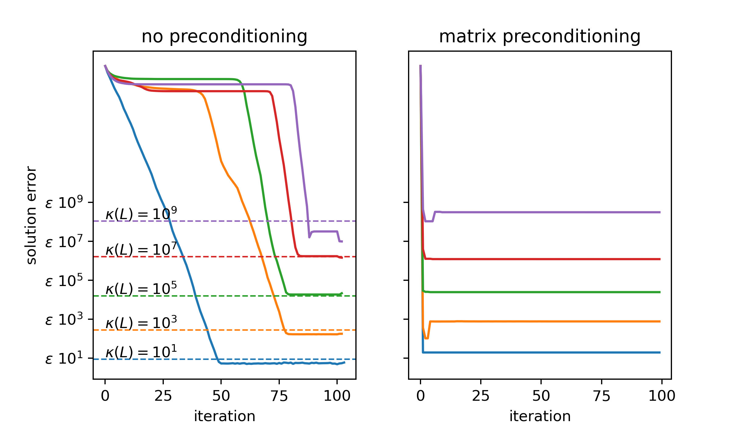
Figure 2.1: Relative error as a function of iteration count for GMRES on linear systems with prescribed condition numbers in $\mathbb{R}^{100\times 100}$. The left panel shows unpreconditioned GMRES, the right preconditioned GMRES with $\mathbf{L}^{-1}$ as the preconditioner. Dashed lines in the left panel indicate the error of the solution obtained with a direct method. Ticks in the y axis are set at $\epsilon\kappa(\mathbf{L})$ for the different used matrices $\mathbf{L}$, where $\epsilon=10^{-16}$ is close to machine precision.

This illustrates that the limiting error of the numerical solution roughly scales linearly with $\kappa(\mathbf{L})$, no matter what algorithm or preconditioner is used.

One exception to this is when special structure in the matrices can be exploited. When tighter bounds than (2.9) hold, matrix preconditioning does improve the condition number and error with the same factor. If, for example, the matrix preconditioner is diagonal, multiplication can be performed row or column-wise with machine accuracy, as no summation of elements is involved. In fact, diagonal preconditioning is often equivalent to one of the simplest forms of FOP, namely, the rescaling of the basis. However, unless such special cases apply, matrix preconditioning only improves the speed of iterative methods.

So far in this section, we have seen that ill-conditioned matrices lead to high numerical error, and that matrix preconditioning does not alleviate this issue. This holds even when the matrix preconditioner improves the convergence of iterative methods as if the preconditioned system has a lower condition number. When error reduction is desired, the only effective alternative is to remove the ill-conditioning altogether. This is what FOP achieves.

With FOP, it is possible to obtain a solution to the original problem but through a different linear system $\tilde{\mathbf{L}}\tilde{\mathbf{u}}=\tilde{\mathbf{b}}$ with significantly lower condition number $\kappa(\tilde{\mathbf{L}})$. The system matrix $\tilde{\mathbf{L}}$ can be obtained precisely, as it is not the result of some potentially ill-conditioned matrix operation. The system can then be solved with improved accuracy (and speed if an iterative solver is used). Coming up with a good preconditioner for FOP is not trivial. However, some rules can guide this process. The next section introduces the framework which will be used to investigate FOP preconditioners.

It is worth reiterating that to improve accuracy with FOP, the goal should always be to reduce the conditioning: If the spectrum is clustered but $\kappa(\mathbf{\tilde{L}})=\kappa(\mathbf{L})$, then only the speed will be improved, and not the accuracy.

2.5 Operator-norm inheritance by discretized matrix

As the condition number is composed of the norm of the matrix and its inverse, both factors need to be bounded to control its growth. Bounding the norm of the inverse, or even ensuring invertibility at all, is often a complex issue that involves additional assumptions in many solution algorithms [7]. Few general statements can be made, and bounds in the following sections are established on a case-by-case basis. On the contrary, simple bounds for the norm of the matrix are available. They are inherited from the boundedness of the operator in the continuous setting. This is known and commonly used in the analysis of Galerkin methods, yet often overlooked in other contexts. We therefore discuss this here in more generality.

As a necessary assumption for most standard stability theorems concerning the solution of the original equation [10, Chapter 6], [12, Chapter 1], we assume the operator $\mathcal{L}:V\rightarrow W$ to be continuous, i.e. there is a constant $C_{\mathcal{L}}>0$ such that

$$\|\mathcal{L}v\|_{W}\leq C_{\mathcal{L}}\|v\|_{V},\quad\text{ for all }v\in V,$$

where $\|\cdot\|_{W}$ and $\|\cdot\|_{V}$ are the norms induced by the scalar products on $W$ and $V$. The infimum of all such constants $C_{\mathcal{L}}$ is called the norm of the operator, and we denote it by $\|\mathcal{L}\|$. Note that this norm depends on the norms of the spaces $V$ and $W$. Since $\|\cdot\|_{W}$ is induced by a scalar product, the norm of $\mathcal{L}$ is given by

$$\|\mathcal{L}\|=\sup_{\begin{subarray}{c}v\in V\\ v\neq 0\end{subarray}}\frac{\|\mathcal{L}v\|_{W}}{\|v\|_{V}}=\sup_{\begin{subarray}{c}w\in W\\ w\neq 0\end{subarray}}\sup_{\begin{subarray}{c}v\in V\\ v\neq 0\end{subarray}}\frac{(w,\mathcal{L}v)_{W}}{\|w\|_{W}\|v\|_{V}}.$$

An analogous statement holds for the norm of a matrix. We formulate it here for the Euclidean norm on $\mathbb{R}^{n}$:

$$\|\mathbf{L}\|_{2}=\max_{\begin{subarray}{c}\mathbf{v}\in\mathbb{R}^{n}\end{subarray}}\frac{\|\mathbf{L}\mathbf{v}\|_{2}}{\|\mathbf{v}\|_{2}}=\max_{\begin{subarray}{c}\mathbf{w}\in\mathbb{R}^{n}\\ \mathbf{w}\neq 0\end{subarray}}\max_{\begin{subarray}{c}\mathbf{v}\in\mathbb{R}^{n}\\ \mathbf{v}\neq 0\end{subarray}}\frac{\mathbf{w}^{\top}\mathbf{L}\mathbf{v}}{\|\mathbf{w}\|_{2}\|\mathbf{v}\|_{2}}.$$

Inserting the definition (2.4) of the matrix-representation of $\mathcal{L}$, we obtain

$$\|\mathbf{L}\|_{2} =\max_{\begin{subarray}{c}\mathbf{w}\in\mathbb{R}^{n}\\ \mathbf{w}\neq 0\end{subarray}}\max_{\begin{subarray}{c}\mathbf{v}\in\mathbb{R}^{n}\\ \mathbf{v}\neq 0\end{subarray}}\frac{\mathbf{w}^{\top}\mathbf{L}\mathbf{v}}{\|\mathbf{w}\|_{2}\|\mathbf{v}\|_{2}}=\max_{\begin{subarray}{c}\mathbf{w}\in\mathbb{R}^{n}\\ \mathbf{w}\neq 0\end{subarray}}\max_{\begin{subarray}{c}\mathbf{v}\in\mathbb{R}^{n}\\ \mathbf{v}\neq 0\end{subarray}}\dfrac{\sum_{j=1}^{n}\sum_{k=1}^{n}(w_{j}\psi_{j},\mathcal{L}v_{k}\phi_{k})_{W}}{\|\mathbf{w}\|_{2}\|\mathbf{v}\|_{2}}$$

$$\leq\|\mathcal{L}\|\max_{\begin{subarray}{c}\mathbf{w}\in\mathbb{R}^{n}\\ \mathbf{w}\neq 0\end{subarray}}\frac{\left\|\sum_{j=1}^{n}w_{j}\psi_{j}\right\|_{W}}{\|\mathbf{w}_{2}\|_{2}}\max_{\begin{subarray}{c}\mathbf{v}\in\mathbb{R}^{n}\\ \mathbf{v}\neq 0\end{subarray}}\frac{\left\|\sum_{k=1}^{n}v_{k}\phi_{k}\right\|_{V}}{\|\mathbf{v}_{2}\|_{2}}$$

$$=\|\mathcal{L}\|\tilde{\Gamma}_{\psi}(n)\tilde{\Gamma}_{\phi}(n).$$ (2.11)

Here, we make use of the fact that on $\mathbb{R}^{n}$ the norms induced by the bases $\phi_{j}$ and $\psi_{k}$ are equivalent to the Euclidean norm. In other words, for each $n\in\mathbb{N}$, there are constants $\tilde{\gamma}_{\phi}(n)\leq\tilde{\Gamma}_{\phi}(n)$ and $\tilde{\gamma}_{\psi}(n)\leq\tilde{\Gamma}_{\psi}(n)$ such that

$$\tilde{\gamma}_{\phi}(n)\|\mathbf{v}\|_{2}\leq\left\|\sum_{k=1}^{n}w_{k}\phi_{k}\right\|_{V}\leq\tilde{\Gamma}_{\phi}(n)\|\mathbf{v}\|_{2},$$

and analogously for $W$. The equivalence of all norms on a finite-dimensional vector space does not mean that these constants do not depend on $n$. In fact, by equation (2.11), the scaling of $\tilde{\Gamma}_{\phi}$ and $\tilde{\Gamma}_{\psi}$ with $n$ is the determining factor for the growth of the norm of the matrix $\mathbf{L}$, as $\|\mathcal{L}\|$ does not depend on $n$. Note that, in addition to $n$, these constants depend on the choice of the basis and on the norm of the spaces $V$ or $W$. Often, results of the form $\tilde{\Gamma}_{\phi}(n)=\Gamma_{\phi}n^{\mu}$ are available, where $\mu\in\mathbb{Z}$, explicitely stating the $n$-dependence of the norm equivalence.

We immediately obtain a desirable criterion for the spaces $V$ and $W$ and for the trial and test functions: The test functions must be chosen such that their growth is limited in the norms on $V$ and $W$, with respect to which $\mathcal{L}$ must be bounded.

One way to guarantee this criterion is by dividing each basis element by their norm. This corresponds to diagonal preconditioning. For some problems, this resolves the problem of exploding norms: See for example [4], who discuss diagonal preconditioning for finite-element methods with highly refined meshes. In other cases, such preconditioning negatively impacts the norm of the inverse of $\mathbf{L}$, and thus leads to minor or no improvements of the condition number. We discuss such an application in Section 5.

The above process shows the beauty of the full operator approach for preconditioning, as important bounds can be derived directly from the operator properties.

3 FOP for polynomial interpolation in $1D$

We begin our discussion with a very simple and well-known numerical task: the polynomial interpolation of a function $f$ on the interval $[-1,1]$ by a polynomial $q$.

In order to formulate this problem, we introduce some notation. For $n\in\mathbb{N}$, let $\mathbb{P}_{n-1}$ be the space of polynomials of degree up to $n-1$, and $\{\operatorname{\mathsf{x}}_{j}\}_{j=1}^{n}$ be a set of $n$ predetermined nodes in $[-1,1]$. For $q\in\mathbb{P}_{n-1}$, we require that $q$ interpolates $f$ at $\{\operatorname{\mathsf{x}}_{j}\}_{j=1}^{n}$:

$$q(\operatorname{\mathsf{x}}_{j})=f(\operatorname{\mathsf{x}}_{j}),\quad\text{ for all }j\in\{1,\dotsc,n\}.$$ (3.1)

By choosing a basis $\{\phi_{i}\}_{i=1}^{n}$ of $\mathbb{P}_{n-1}$, we can write the interpolant $q\in\mathbb{P}_{n-1}$ as $q(x)=\sum_{j=1}^{n}q_{j}\phi_{j}(x)$. Then, plugging this into (3.1), we obtain the linear system

$$\underbrace{\begin{pmatrix}\phi_{0}(\operatorname{\mathsf{x}}_{1})&\phi_{1}(\operatorname{\mathsf{x}}_{1})&\dotsc&\phi_{n-1}(\operatorname{\mathsf{x}}_{1})\\ \phi_{0}(\operatorname{\mathsf{x}}_{2})&\ddots&&\phi_{n-1}(\operatorname{\mathsf{x}}_{2})\\ \vdots&&\ddots&\vdots\\ \phi_{0}(\operatorname{\mathsf{x}}_{n})&\phi_{1}(\operatorname{\mathsf{x}}_{n})&\dotsc&\phi_{n-1}(\operatorname{\mathsf{x}}_{n})\end{pmatrix}}_{=:\mathbf{L}_{\phi}}\begin{pmatrix}q_{0}\\ q_{1}\\ \vdots\\ q_{n-1}\end{pmatrix}=\begin{pmatrix}f(\operatorname{\mathsf{x}}_{1})\\ f(\operatorname{\mathsf{x}}_{2})\\ \vdots\\ f(\operatorname{\mathsf{x}}_{n})\end{pmatrix}$$ (3.2)

for the coefficients of $q$. We call $\mathbf{L}_{\phi}\in\mathbb{R}^{n\times n}$ the interpolation matrix (with respect to the basis $\{\phi_{i}\}_{i=0}^{n-1}$). If the interpolation nodes $\{\operatorname{\mathsf{x}}_{j}\}_{j=1}^{n}$ satisfy $\operatorname{\mathsf{x}}_{i}\neq\operatorname{\mathsf{x}}_{k}$ for $i\neq k$, then (3.2) has a unique solution [2, Theorem 3.1]. However, we point out that the condition number of the matrix $\mathbf{L}_{\phi}$ determines the accuracy and speed with which the linear system can be solved.

A straightforward choice for the basis for $\mathbb{P}_{n-1}$ is the set of monomials $\{\mu_{i}\}_{i=0}^{n-1}$, where $\mu_{i}(x):=x^{i},\>i\in\mathbb{N}_{+}:=\mathbb{N}\cup\{0\}$. Under this choice, the matrix $\mathbf{L}_{\mu}$ is called the Vandermonde matrix of the points set $\{\operatorname{\mathsf{x}}_{j}\}_{j=1}^{n}$. Unfortunately, despite the simplicity of its structure, it is known for being notoriously hard to solve [19]. In fact, for most choices of $\operatorname{\mathsf{x}}_{j}\in\mathbb{R}$, the condition number of the Vandermonde matrix can be shown to grow at least exponentially in $n$ [5].

Other combinations of basis polynomials and interpolation points can lead to better condition numbers. Consider, for instance, the Chebyshev polynomials of the first kind, defined by

$$T_{k}(x)=\cos(k\arccos(x)),\qquad x\in[-1,1],\>k\in\mathbb{N}_{+}.$$

Note that for each $k\in\mathbb{N}_{+}$, $T_{k}$ is a polynomial of degree $k$ [46, Chapter 3]. Thus, $\{T_{k}\}_{k=0}^{n-1}$ forms a basis of the space $\mathbb{P}_{n-1}$. Therefore, we can define $\mathbf{L}_{T(n)}$ as the interpolation matrix constructed using $\{T_{i}\}_{i=0}^{n-1}$ and the degree-$n$ Chebyshev nodes

$$\operatorname{\mathsf{x}}_{j}=\cos\left(\frac{2j-1}{2(n+1)}\right),\quad\text{ for }j\in\{1,\dotsc,n\},$$ (3.3)

as interpolation nodes. It is known that the matrix $\mathbf{L}_{T(n)}$ is well conditioned [43] with $\kappa\left(\mathbf{L}_{T}(n)\right)=\sqrt{2}$ for all $n\in\mathbb{N}$.

Although these facts about $\mathbf{L}_{\mu}$ and $\mathbf{L}_{T(n)}$ are well known, we believe that FOP brings a new insight as to why one system behaves numerically so much better than the other.

3.1 Polynomial interpolation as discretization of an operator equation

The task of polynomial interpolation can be understood as discretizing the operator equation

$$\mathcal{I}u=f,$$

with the identity operator $\mathcal{I}$ and a particular choice of (suitable) trial and test spaces $V$ and $W$, respectively. Let $\{\phi_{i}\}_{i=0}^{n-1}$ be a basis of $\mathbb{P}_{n-1}$ and define the trial-space basis operator $\mathcal{X}_{\phi}:\mathbb{R}^{n}\rightarrow\mathbb{P}_{n-1}$ as

$$\mathcal{X}_{\phi}\mathbf{u}=\sum_{k=0}^{n-1}u_{k}\phi_{k}.$$

Further, let $\{\operatorname{\mathsf{x}}_{j}\}_{j=1}^{n}$ be the set of $n$ interpolation points. We define the test operator $\mathcal{W}_{\operatorname{\mathsf{x}}}:W\rightarrow\mathbb{R}^{n}$ as

$$\mathcal{W}_{\operatorname{\mathsf{x}}}f=(\delta_{\operatorname{\mathsf{x}}_{1}}(f),\dotsc,\delta_{\operatorname{\mathsf{x}}_{n}}(f))^{\top},$$

where $\delta_{\operatorname{\mathsf{x}}}$ is the delta distribution centered at the point $\operatorname{\mathsf{x}}$. Then, the linear system (3.2) for this discretization can be rewritten as

$$\mathbf{L}_{\phi}\mathbf{q}=\mathbf{f},$$ (3.4)

with $\mathbf{f}=\mathcal{W}_{\operatorname{\mathsf{x}}}f$, and $\mathbf{L}[i,j]:=(\mathcal{W}_{\operatorname{\mathsf{x}}}\mathcal{I}\mathcal{X}_{\phi})[i,j]=\delta_{\operatorname{\mathsf{x}}_{j}}(\phi_{i})$ for $i\in\{0,\dots,n-1\},j\in\{1,\dots,n\}.$

It is clear that choosing a different basis $\{\Phi_{i}\}_{i=0}^{n-1}$ for $\mathbb{P}_{n-1}$ defines a new trial-space basis operator $\mathcal{X}_{\Phi}$ and also a new matrix $\mathbf{L}_{\Phi}=\mathcal{W}_{\operatorname{\mathsf{x}}}\mathcal{I}\mathcal{X}_{\Phi}$.

3.2 FOP vs. matrix preconditioning

Now suppose that $\mathbf{L}_{\phi}$ is ill-conditioned, whereas $\mathbf{L}_{\Phi}$ is well-conditioned. Then it is desirable to solve systems involving the matrix $\mathbf{L}_{\Phi}$ rather than $\mathbf{L}_{\phi}$. This can be achieved by right-preconditioning: instead of solving (3.4), we work with

$$\mathbf{L}_{\Phi}\mathbf{v}=\mathbf{L}_{\phi}\mathbf{R}_{\Phi}^{\phi}\mathbf{v}=\mathbf{f},$$

where $\mathbf{R}_{\Phi}^{\phi}=\mathcal{X}_{\phi}^{-1}\mathcal{X}_{\Phi}\in\mathbb{R}^{n\times n}$ is the basis transformation from $\{\Phi_{i}\}_{i=0}^{n-1}$ to $\{\phi_{i}\}_{i=0}^{n-1}$. One could then obtain the original vector $\mathbf{q}=\mathbf{R}_{\Phi}^{\phi}\mathbf{v}$, though this could involve an ill-conditioned basis transformation (so it is advisable to work with the well-conditioned basis $\Phi$ as much as possible).

There are two options to implement such right preconditioning. One the one hand, one could employ matrix preconditioning, i.e. discretizing first, and multiplying the matrices afterward. When the matrices $\mathbf{L}_{\phi}$ and $\mathbf{R}_{\Phi}^{\phi}$ are known, this amounts to numerical matrix multiplication $\mathbf{L}_{\phi}\mathbf{R}_{\Phi}^{\phi}$ for direct solution or the application of an iterative solver employing one matrix-vector multiplication with both $\mathbf{L}_{\phi}$ and $\mathbf{R}_{\Phi}^{\phi}$ per iteration. On the other hand, one could compute the matrix $\mathbf{L}_{\Phi}$ directly—in this case by evaluating the polynomial basis $\Phi_{k}$ at the interpolation nodes—and employing a numerical solver, which avoids matrix multiplication with $\mathbf{L}_{\phi}$. Almost always, the first alternative does nothing to improve the accuracy of the final result.

Let us illustrate this with $\mathbf{L}_{\mu}$ and $\mathbf{L}_{T(n)}$. For this, the matrix $\mathbf{C}:=\mathbf{R}_{\mu}^{T(n)}$ can be computed explicitly, e.g. [46, Ch. 2]. Therefore, a polynomial in $\mathbb{P}_{n-1}$ given by its vector of coefficients $\mathbf{u}\in\mathbb{R}^{n}$ in the Chebyshev basis has coefficients $\mathbf{C}^{\top}\mathbf{u}=(\mathcal{X}_{\mu}^{-1}\mathcal{X}_{T(n)})\mathbf{u}$ in the monomial basis.

We proceed to compare solving $\mathbf{L}_{\mu}\mathbf{x}=\mathbf{b}$ and $\mathbf{L}_{T(n)}\mathbf{x}=\mathbf{b}$ with GMRES. We start by generating a function with prescribed coefficients in the monomial basis $\sum_{k=0}^{n-1}q_{k}\phi_{k}$ in which the coefficients are drawn from the standard normal distribution $q_{k}\sim N(0,1)$, and compute the right-hand side $f(\operatorname{\mathsf{x}}_{1})$ via (3.2), taking $\operatorname{\mathsf{x}}_{i}$ to be the Chebyshev nodes (3.3). We then solve the linear system (3.2) using (a maximum of $n$ steps of) GMRES, without and with right preconditioning $\mathbf{C}$. As the focus is to examine the best possible accuracy, we ran GMRES with the tightest tolerance: the convergence tolerance is set to $\epsilon$ and maximum number of iteration $n$. For reference we also present the analogous result with (well-conditioned) Chebyshev coefficients (without preconditioning), wherein the ’exact’ coefficients are obtained using Chebfun [16]. The results are shown in Figure 3.1.

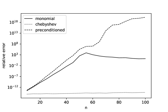
Figure 3.1: Relative 2-errors of the computed solutions averaged over 100 draws. Solutions for $\mathbf{L}_{\mu}\mathbf{x}=\mathbf{b}$ (monomial basis, with and without preconditioner $\mathbf{C}$), and $\mathbf{L}_{T(n)}\mathbf{x}_{T}=\mathbf{b}$ (Chebyshev basis) were obtained with GMRES. $\mathbf{x}$ and $\mathbf{q}$ are sampled randomly from an $n$-dimensional standard normal distribution, and the same right-hand side $\mathbf{b}$ is used for the three linear systems.

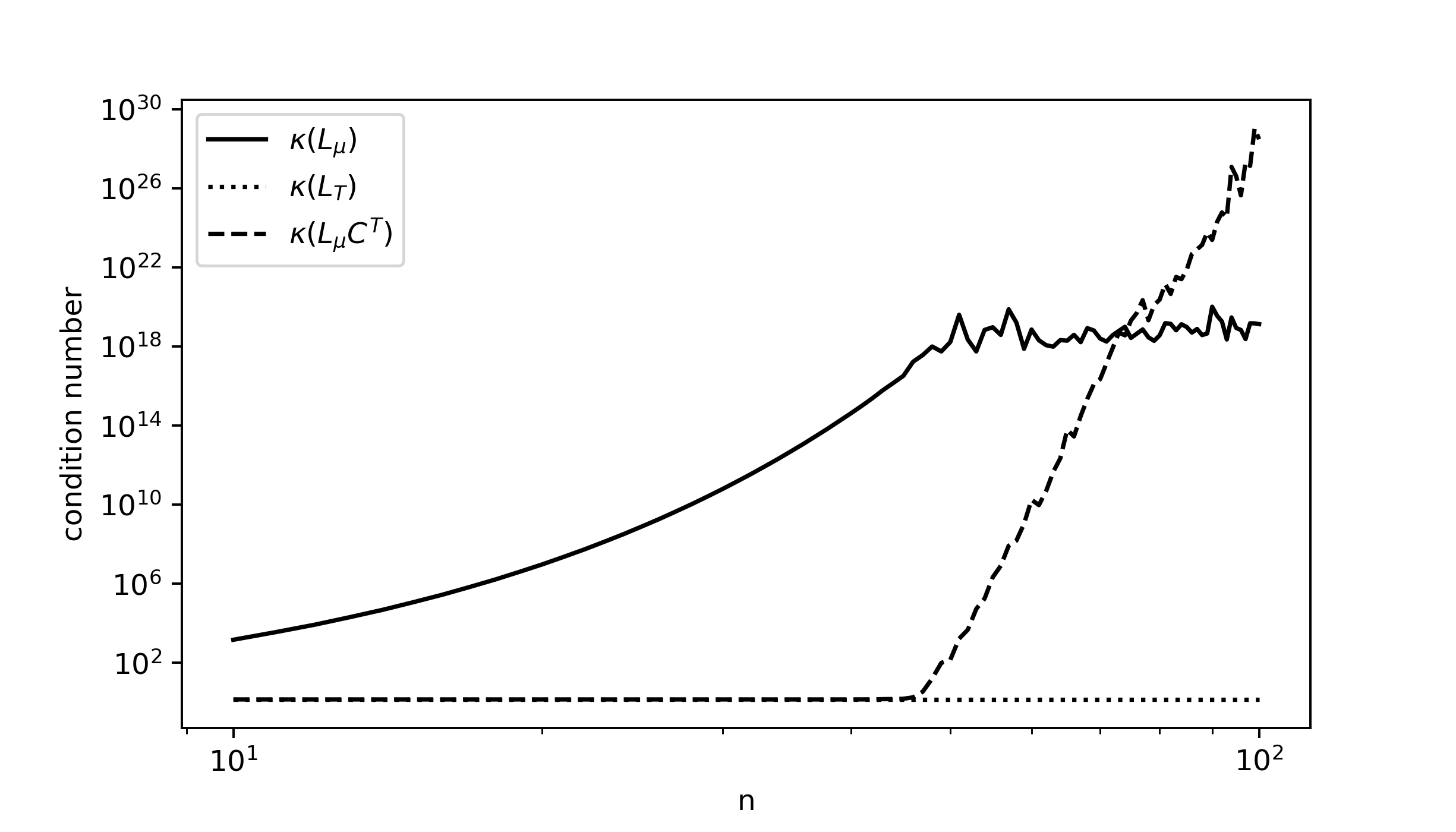
Figure 3.2: Condition numbers of $\mathbf{L}_{\mu}$, $\mathbf{L}_{T(n)}$ and $\mathbf{L}_{\mu}\mathbf{C}^{\top}$.

As expected, numerical error limits the use of matrix-level preconditioning for improving accuracy. Figure 3.2 shows the condition numbers of the monomial interpolation matrix $\mathbf{L}_{\mu}$, the Chebyshev interpolation matrix $\mathbf{L}_{T(n)}$, and the matrix obtained by multiplying $\mathbf{L}_{\mu}$ and $\mathbf{C}^{\top}$ with finite-precision arithmetic for $n$ up to $70$. $\mathbf{C}$ is obtained by the above recursion relation. As expected, the condition number of the Vandermonde matrix $\kappa(\mathbf{L}_{\mu})$ grows exponentially, while $\kappa(\mathbf{L}_{T(n)})$ stays constant. Matrix preconditioning is stable until $n\approx 45$, beyond which the associated condition number increases unpredictably, even surpassing that of the original matrix $\mathbf{L}_{\mu}$. As the condition number $\kappa(\mathbf{L}_{\mu})$ climbs to $10^{18}>1/\epsilon$, neither $\kappa(\mathbf{L}_{\mu})$ nor the condition number of the product with the preconditioner can be expected to be numerically accurate. This explains the flattening of $\kappa(\mathbf{L}_{\mu})$.

3.3 Analysis and Discussion

In order to study the condition numbers of interest, we make use of the fact that $\kappa(\mathbf{L})=\|\mathbf{L}\|_{2}\|\mathbf{L}^{-1}\|_{2}$ and turn our attention to the norm of the matrices $\mathbf{L}_{\mu}$, $\mathbf{L}_{T(n)}$ and their inverses. Moreover, we leverage the operator perspective from (3.4) to find estimates for these norms following the spirit of equation (2.11).

First, the Sobolev embedding theorem guarantees that functions $f\in H^{1}(-1,1)$ are almost everywhere equal to a continuous function. Moreover, there is a constant $\alpha>0$, independent of $f$, such that [36, Chapter 7]

$$\|f\|_{L^{\infty}(-1,1)}\leq\alpha\|f\|_{H^{1}(-1,1)},\quad\text{ for all }f\in H^{1}(-1,1).$$ (3.5)

By letting the delta distributions act on the continuous representation of functions in $H^{1}(-1,1)$, they belong to the space $H^{-1}(-1,1)$ with norm

$$\|\delta_{\operatorname{\mathsf{x}}_{j}}\|_{H^{-1}(-1,1)}=\sup_{v\in H^{1}(-1,1)}\frac{\delta_{\operatorname{\mathsf{x}}_{j}}(v)}{\|v\|_{H^{1}(-1,1)}}\leq\sup_{v\in H^{1}(-1,1)}\frac{\|v\|_{L^{\infty}(-1,1)}}{\|v\|_{H^{1}(-1,1)}}\leq\alpha.$$ (3.6)

Then, for any interpolation basis $\{\phi_{i}\}_{i=1}^{n}$ in $H^{1}(-1,1)$, we obtain

$$\begin{split}\|\mathbf{L}_{\phi}\|_{2}&=\max_{\mathbf{v}\in\mathbb{R}^{n}}\max_{\mathbf{w}\in\mathbb{R}^{n}}\frac{\mathbf{w}^{\top}\mathbf{L}_{\phi}\mathbf{v}}{\|\mathbf{w}\|_{2}\|\mathbf{v}\|_{2}}=\max_{\mathbf{v}\in\mathbb{R}^{n}}\max_{\mathbf{w}\in\mathbb{R}^{n}}\sum_{j,k}\frac{w_{j}v_{k}\delta_{\operatorname{\mathsf{x}}_{j}}(\phi_{k})}{\|\mathbf{w}\|_{2}\|\mathbf{v}\|_{2}}\\ &\leq\max_{\mathbf{v}\in\mathbb{R}^{n}}\max_{\mathbf{w}\in\mathbb{R}^{n}}\sum_{j,k}\frac{w_{j}v_{k}\alpha\|\phi_{k}\|_{H^{1}(-1,1)}}{\|\mathbf{w}\|_{2}\|\mathbf{v}\|_{2}}\leq\alpha\max_{1\leq l\leq n}\|\phi_{l}\|_{H^{1}(-1,1)},\end{split}$$

where in the last line, we used (3.5) and the Cauchy-Schwarz inequality.

For the monomials in $[-1,1]$, since $\delta(\phi_{k})\leq 1$, this estimate is easily improved to $\|\mathbf{L}_{\mu}\|\leq n$, which is still not sharp. Thus, the norm of $\mathbf{L}_{\mu}$ is relatively well-behaved. This implies that the exponential increase in the condition number of the Vandermonde matrix $\kappa(\mathbf{L}_{\mu})$ comes from the contribution of the inverse, i.e., the presence of small singular values.

Remark 3.1.

We observe that the boundedness of the condition number results from two key properties:

• the orthogonality of the columns in the interpolation matrix; and

• the controlled behavior of the norms of the columns.
  

In view of (P1), one could want to extend the idea of orthogonal-column interpolation matrices $\mathbf{L}_{\Phi}$ to other choices of trial bases. This can easily be done for other orthogonal polynomials, see [37] for a detailed discussion.

4 FOP for spectral methods

In the next two sections, we give examples of FOP in the context of differential equations. In this section, we focus on spectral methods, and we turn to finite element methods in the next.

Spectral methods are known for their excellent convergence properties [44, Chapter 4]. If the solution of the problem is analytic, the error decreases faster than any negative power of the discretization size. However, in their most straightforward implementation, spectral methods suffer from a fast increase of the condition number, leading to slow convergence and numerical instabilities. For high-order differential operators, or if high accuracy is desired, this quickly becomes prohibitive. The combination of these properties makes spectral methods ideal candidates for FOP.

Several preconditioning techniques have been presented in the literature. Basic examples include low-order finite element or finite difference preconditioners, or spectral discretizations of the differential operator with variable coefficients replaced by constants [10, § 4.4]. These methods rely on linear operations which can only be computed with finite precision. As discussed in Section 2.4 and exemplified in Section 3.2, preconditioning only improves accuracy if no multiplication between ill-conditioned matrices takes place.

One family of methods that achieve accuracy improvement is known as integration preconditioning [39]. These methods use relations between the spectral basis and the derivatives of its elements, which under certain conditions form orthogonal global bases on their own. An early version of integration preconditioning was presented by Clenshaw [13], and the method was later developed in [14, 15, 17]. We focus here on one particular realization given by Olver and Townsend [39], which uses the relationship between Chebyshev and ultraspherical polynomials. We add a new viewpoint to the analysis by explicitly formulating the operators that are used for FOP. This allows us to identify them as generalized integral operators and to show they meet the desired criteria laid out in Section 2.5.

4.1 Unpreconditioned spectral methods

Let $\mathcal{L}$ be a linear differential operator of order $N$. As before, we limit ourselves to the interval $[-1,1]$. We assume the leading-order coefficient to be non-singular, so that without limitation of generality we may write the operator in normalized form

$$\mathcal{L}=\frac{d^{N}}{dx^{N}}+a_{N-1}\frac{d^{N-1}}{dx^{N-1}}+\dots+a_{1}\frac{d^{1}}{dx^{1}}+a_{0},$$ (4.1)

with continuous functions $a_{N-1},\dots,a_{0}:[-1,1]\rightarrow\mathbb{R}$.

We want to solve the problem

$$\begin{split}\mathcal{L}u=f,\quad\text{ for }x\in(-1,1),\quad\text{ such that }\mathcal{B}u=\mathbf{c},\end{split}$$

where $f:[-1,1]\rightarrow\mathbb{R}$, $\mathbf{c}\in\mathbb{R}^{N}$ and $\mathcal{B}$ is a linear operator imposing $N$ linearly independent (boundary) constraints on the solution $u$.

Choosing Chebyshev polynomials $\phi_{k}=T_{k}$ as the trial basis, we search for an approximate solution in the finite-dimensional space $V_{n}=\text{span}\{\phi_{i}\}_{i=0}^{n-1}$. As the trial basis, projection onto the functions $T_{k}/\|T_{k}\|_{L^{2}(\rho)}^{2}$ is common, which decomposes the result of the application of the differential operator in terms of the Chebyshev polynomials and leads to the representation matrix

$$\mathbf{L}[i,j]=\frac{(\phi_{i},\mathcal{L}\phi_{j})_{L^{2}(\rho)}}{\|\phi_{i}\|_{L^{2}(\rho)}^{2}}.$$

For this choice, differentiation is represented by a dense upper-triangular matrix $\mathbf{D}$, found for example in [21]. Further, due to the convolution formula for Chebyshev polynomials

$$2T_{m}T_{k}=T_{m+k}+T_{|m-k|},$$ (4.2)

multiplication with polynomial coefficient functions $a_{j}$ is replaced by multiplication with banded matrices $\mathbf{M}(a_{j})$ with bandwidth $2\text{ deg}(a_{j})+1$ [14]. Nonpolynomial functions are first expanded in terms of Chebyshev polynomials up to machine accuracy and then converted into matrix form.

To make the solution of the system of equations unique, boundary conditions need to be incorporated. For this, we make use of the method of boundary bordering: The last $N$ rows of the $n\times n$ matrix $\mathbf{L}$ are omitted and replaced, conventionally swapped to the top of the linear system, by the $N$ linearly independent equations coming from the application of $\mathcal{B}$ to the approximation $u=\sum u_{j}\phi_{j}$. We denote the matrix $\mathbf{L}$ with the last $N$ rows left out as $\mathbf{L}_{[N]}$, such that we obtain the system $\mathbf{A}\mathbf{u}=\mathbf{b}$ with

$$\mathbf{A}:=\begin{pmatrix}\mathcal{B}\phi_{0}&\mathcal{B}\phi_{1}&\dots&\mathcal{B}\phi_{n-1}\\ \mathbf{L}_{[N]}\end{pmatrix},\>\text{ and }\>\mathbf{b}:=\begin{pmatrix}\mathbf{c}\\ (\psi_{0},f)/(\psi_{0},\psi_{0})\\ \ldots\\ (\psi_{n-N-1},f)/(\psi_{n-N-1},\psi_{n-N-1})\end{pmatrix}.$$

As a specific example, consider the differential equation

$$\frac{d^{2}}{dx^{2}}u+10\frac{d}{dx}u+100\,x\,u=f,\quad\text{ such that }u(\pm 1)=0.$$ (4.3)

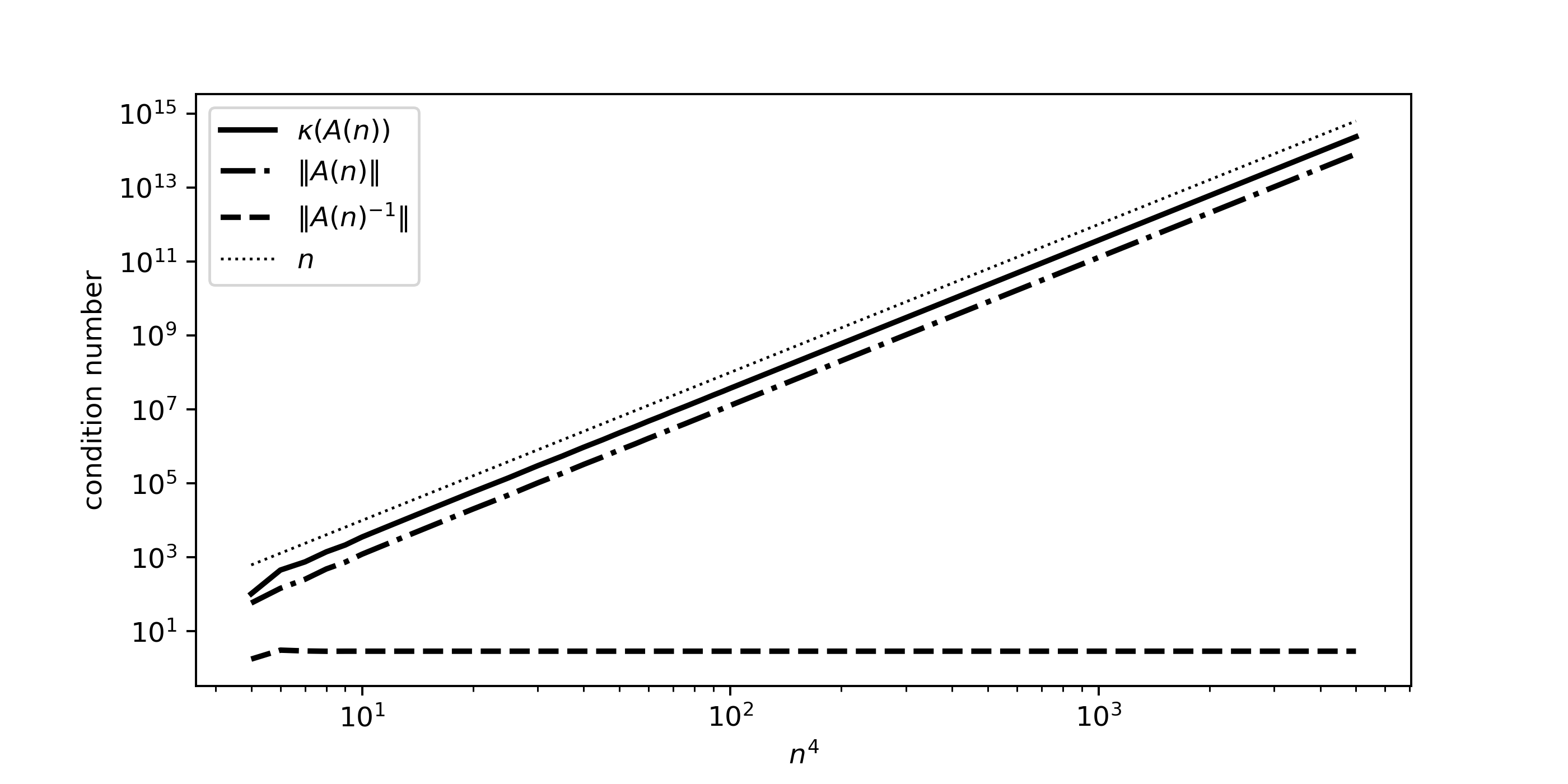
Figure 4.1: Condition number $\kappa(\mathbf{A})$ and norms $\|\mathbf{A}\|_{2}$ and $\|\mathbf{A}^{-1}\|_{2}$ of the spectral representation matrix with Chebyshev basis for the differential equation (4.3) with Dirichlet boundary conditions.

Figure 4.1 shows the condition number of $\mathbf{A}$ as a function of the discretization size. We confirm that it increases as $\mathcal{O}(n^{2N})$ for a differential operator of order $N$ as predicted for Chebyshev polynomials [8, § 7.7]. Also displayed in the figure are the $2$-norms of the matrix $\mathbf{A}$ and of its inverse. While $\|\mathbf{A}^{-1}\|_{2}$ is nearly constant, the factor $\|\mathbf{A}\|_{2}$ is responsible for the rapid growth of the condition number $\kappa(\mathbf{A})=\|\mathbf{A}\|_{2}\|\mathbf{A}^{-1}\|_{2}$. Far from conclusive for general differential equations, this example shows that bounds on the norm of the matrix $\mathbf{L}$, such as the bound (2.11) inferred from the continuity of the operator, can be of use in the development and understanding of preconditioners.

4.2 Ultraspherical polynomials

As already shown in Section 3, structural properties of matrices representing the same operator but obtained with different trial and test bases may differ fundamentally. The method presented in [39] is a beautiful example of this. Retaining Chebyshev polynomials as the trial-space basis, they switch the test-space basis to ultraspherical polynomials, thereby reducing the growth of the condition number from $\mathcal{O}(n^{2N})$ to $\mathcal{O}(n)$.

Futher, this may be seen as an application of FOP: The three operations involved in constructing the spectral matrix $\mathbf{L}$—differentiation, multiplication and basis change—may be computed by a recursion. This allows the computation of the preconditioned matrix without any ill-conditioned matrix multiplication.

For $\lambda\in\mathbb{N}$, the ultraspherical polynomials $(C^{(\lambda)}_{k})_{k\in\mathbb{N}}$ of order $\lambda$ are defined as the family of polynomials orthogonal with respect to the $L^{2}$-scalar product with weight

$$\rho^{(\lambda)}(x)=(1-x^{2})^{\lambda-1/2},\quad x\in(-1,1)$$

and normalized such that

$$C^{(\lambda)}_{k}(x)=\frac{2^{k}(\lambda+k-1)!}{(\lambda-1)!k!}x^{k}+\mathcal{O}(x^{k-1}).$$

Together with the Chebyshev polynomials, they fulfill the defining properties

$$\frac{dC^{(\lambda)}}{dx}=\begin{cases}2\lambda C^{(\lambda+1)}_{k-1},\quad&\text{ for }k\geq 1,\\ 0,\quad&\text{ for }k=0.\end{cases}\quad\text{ and }\quad\frac{dT_{k}}{dx}=\begin{cases}kC^{(1)}_{k-1},\quad&\text{ for }k\geq 1,\\ 0,\quad&\text{ for }k=0,\end{cases}$$ (4.4)

such that $\lambda$-fold differentiation between Chebyshev and order-$\lambda$ ultraspherical polynomials is represented by the matrix

$$\mathbf{D}_{\lambda}=2^{\lambda-1}(\lambda-1)!\left(\begin{array}[]{rrrrrrr}\makebox[0.0pt][l]{$\smash{\overbrace{\phantom{\begin{matrix}0&\dots&0\end{matrix}}}^{\text{$\lambda\text{times}$}}}$}0&\dots&0&\lambda&&&\\ &&&&\lambda+1&&\\ &&&&&\lambda+2&\\ &&&&&&\ddots\end{array}\right)$$ (4.9)

To compute the matrix representation $\tilde{\mathbf{L}}$ of the operator $\mathcal{L}$, coefficient functions $a_{j}$ are resolved to machine accuracy in terms of ultraspherical polynomials of order $j$. Due to a convolution formula similar to that for Chebyshev polynomials (4.2), multiplication by the expansion of $a_{j}$ can be written as a matrix $\mathbf{M}_{j}(a_{j})$ acting on the coefficients of an order-$j$ ultraspherical series, see equations (3.6) to (3.9) in [39]. Coefficients of a $C^{(\lambda)}$-series are converted to a $C^{(\lambda+1)}$-series by applying the matrix

$$\mathbf{S}_{\lambda}=\begin{pmatrix}1&&-\frac{\lambda}{\lambda+2}&&&\\ &\frac{\lambda}{\lambda+1}&&-\frac{\lambda}{\lambda+3}&&\\ &&\frac{\lambda}{\lambda+2}&&-\frac{\lambda}{\lambda+4}&\\ &&&\ddots&&\ddots\end{pmatrix},$$ (4.10)

to its vector of coefficients while a Chebyshev series can be converted to a $C^{(1)}$-series with the operator

$$\mathbf{S}_{0}=\begin{pmatrix}1&&-\frac{1}{2}&&&\\ &\frac{1}{2}&&-\frac{1}{2}&&\\ &&\frac{1}{2}&&-\frac{1}{2}&\\ &&&\ddots&&\ddots\end{pmatrix}.$$ (4.11)

Combining these steps, the differential operator is found by computing

$$\tilde{\mathbf{L}}=\mathbf{D}_{N}+\mathbf{S}_{N-1}\mathbf{M}_{N-1}(a_{N-1})\mathbf{D}_{N-1}+\dots+\mathbf{S}_{N-1}\dots\mathbf{S}_{0}\mathbf{M}_{0}(a_{0})$$ (4.12)

The matrices $\mathbf{D}_{j}$ are composed of a single off-diagonal, while the matrices $\mathbf{S}_{j}$ constist of the main-diagonal and one off-diagonal. This results in a banded matrix $\tilde{\mathbf{L}}$.

As before, this matrix is truncated to size $(n-N)\times n$ and complemented with the $N$ boundary conditions to obtain the system matrix $\tilde{\mathbf{A}}(n)$. Numerical experiments indicate that the condition number of these matrices grow as $\mathcal{O}(n)$ [39, § 3.3]. Applying the diagonal preconditioner

$$\mathbf{R}=\frac{1}{2^{j-1}(j-1)!}\,\text{diag}\left(\underbrace{1,\dotsc,1}_{N\text{ times}},\frac{1}{N},\frac{1}{N+1},\dotsc\right)$$ (4.13)

from the right, it is shown in [39, § 4] that

$$\mathbf{A}\mathbf{R}=\mathbf{I}+\mathbf{K}_{n},$$ (4.14)

where sequence of $n\times n$ matrices $\mathbf{K}_{n}$ converges to a compact operator $\mathcal{K}:\ell_{\lambda}^{2}\rightarrow\ell_{\lambda}^{2}$ between the Hilbert spaces

$$\ell_{\lambda}^{2}=\left\{\mathbf{u}=(u_{k})_{k\in\mathbb{N}}:\|\mathbf{u}\|_{\ell_{\lambda}^{2}}=\sqrt{\sum_{k=0}^{\infty}u_{k}^{2}(1+k^{2})^{\lambda}}\right\},$$

and the range of possible $\lambda$ determined by the boundary conditions $\mathcal{B}$. For Dirichlet boundary conditions, this includes $\lambda=0$. By uniform convergence of orthogonal projection in the spectral bases, if $\mathcal{I}+\mathcal{K}$ is invertible, the condition number of the matrices $\mathbf{A}\mathbf{R}$ in the relevant $\ell_{\lambda}^{2}$-norm converges to that of $\mathcal{I}+\mathcal{K}$ [39, § 4]. In other words, growth of the condition number as $n\rightarrow\infty$ has been improved from $\mathcal{O}(n^{2N})$ to $\mathcal{O}(1)$ by a change of basis and the multiplication with a diagonal operator $\mathbf{R}$.

4.3 Basis change as FOP

While it is clear that the application of the operator $\mathcal{R}$ can be seen as a form of FOP, the FOP present in the basis change needs explicit formulation. We define the basis-change preconditioner

$$\mathcal{R}_{l}(C^{(N)}_{k})=T_{k},$$ (4.15)

mapping an ultraspherical polynomial of order $N$ and degree $k$ to the Chebyshev polynomial of degree $k$. By extending $\mathcal{R}_{l}$ to linear combinations and then to series, the operator is well-defined on the space of $L^{2}(\rho^{(N)})$ with weight $\rho^{(N)}(x)=(1-x^{2})^{N-1/2}$.

Applying this operator from the left to the original equation $\mathcal{L}u=f$ and decomposing in terms of the Chebyshev test basis with the $\rho^{(0)}$-scalar product leads to the same matrix as decomposing the original equation directly in terms of the ultraspherical test basis with the $\rho^{(N)}$-scalar product: Recall that the pure-Chebyshev method leads to the matrix

$$\mathbf{L}[j,k]=\frac{(T_{j},\mathcal{L}T_{k})_{L^{2}(\rho^{(0)})}}{\|T_{j}\|^{2}_{L^{2}(\rho^{(0)})}},$$

while the Chebyshev-ultraspherical method results in

$$\tilde{\mathbf{L}}[j,k]=\frac{(C^{(N)}_{j},\mathcal{L}T_{k})_{L^{2}(\rho^{(N)})}}{\|C^{(N)}_{j}\|^{2}_{L^{2}(\rho^{(N)})}}.$$

Multiplying the original equation with $\mathcal{R}_{l}$ and using the pure-Chebyshev formula, we obtain

$$\begin{split}\frac{(T_{j},\mathcal{R}_{l}\mathcal{L}T_{k})_{L^{2}(\rho^{(0)})}}{\|T_{j}\|^{2}_{L^{2}(\rho^{(0)})}}&=\frac{(T_{j},\mathcal{R}_{l}\sum_{m=0}^{\infty}C_{m}^{(N)}\tilde{\mathbf{L}}[m,k])_{L^{2}(\rho^{(0)})}}{\|T_{j}\|^{2}_{L^{2}(\rho^{(0)})}}\\ &=\sum_{m=0}^{\infty}\frac{(T_{j},T_{m}\tilde{\mathbf{L}}[m,k])_{L^{2}(\rho^{(0)})}}{\|T_{j}\|^{2}_{L^{2}(\rho^{(0)})}}=\tilde{\mathbf{L}}[j,k],\end{split}$$ (4.16)

the same matrix as in the Chebyhsev-ultraspherical case.

Hence, the basis change between Chebyshev and ultraspherical polynomials is a case of operator FOP. Together with the right-preconditioner

$$\mathcal{R}_{r}(T_{k})=\frac{1}{2^{N-1}(N-1)!}\begin{cases}T_{k},\quad\text{ if }k<N,\\ \frac{T_{k}}{k},\quad\text{ if }k\geq N,\end{cases}$$ (4.17)

it serves to bound the operator $\mathcal{L}$ on the space $L^{2}(\rho^{(0)})$. Without preconditioning, the order-$N$ differential operator $\mathcal{L}$ is unbounded as an operator $\mathcal{L}:L^{2}(\rho^{(0)})\rightarrow L^{2}(\rho^{(0)})$. After applying preconditioners from the left and the right, it is shown that the representation in terms of Chebyshev polynomials of the operator $\mathcal{R}_{l}\mathcal{L}\mathcal{R}_{r}:L^{2}(\rho^{(0)})\rightarrow L^{2}(\rho^{(0)})$ equals the identity plus a compact operator. By the isometry between $L^{2}(\rho^{(0)})$ and $\ell^{2}$, this implies the continuity of $\mathcal{R}_{l}\mathcal{L}\mathcal{R}_{r}$.

In fact, the two preconditioners serve as an $N$-fold integration, inverting the $N$-th derivative

$$\mathcal{R}_{l}\frac{d^{N}}{dx^{N}}\mathcal{R}_{r}=\mathcal{I}:L^{2}(\rho^{(0)})\rightarrow L^{2}(\rho^{(0)}).$$

In this, aside from providing the factor $1/(2^{N-1}(N-1)!)$, the right preconditioner serves to counteract an assymetry in the definition of Chebyshev and ultraspherical polynomials. While the differentiation of an ultraspherical polynomial $C^{(\lambda)}_{k}$ does not lead to a factor depending on the degree $k$ of the polynomial, differentiating the Chebyshev polynomial $T_{k}$ does. This single linear scaling coming from the first change from $T_{k}$ to $C^{(1)}_{k}$-series is cancelled by $\mathcal{R}_{r}$.

In infinite-precision arithmetic, traditional matrix preconditioning with the truncated diagonal operator $\mathcal{R}$ from the right and the matrix version of $\mathcal{R}_{l}$ with entries

$$\mathbf{R}_{l}[j,k]=(T_{j},\mathcal{R}_{l}(T_{k}))_{L^{2}(\rho^{(0)})}$$

from the left would lead to a solution equivalent to that of the Chebyshev-ultraspheri-cal method. Given that precision is infinite, numerical error does not play a role, and a speedup of iterative methods would occur as predicted by the condition-number improvement induced by the preconditioning. In finite-precision arithmetic, this suffers from the multiplication of the ill-conditioned matrices $\mathbf{L}$ and $\mathbf{R}_{l}$.

For FOP it is thus crucial that the matrix $\tilde{\mathbf{L}}$ is computed to machine precision by use of recursion relations as in equation (4.12) instead of by evaluating the matrix product $\tilde{\mathbf{L}}=\mathbf{R}_{l}\mathbf{L}$.

Similarly, the right-hand side $f$ has to be discretized directly in terms of ultraspherical polynomials. The alternative, a conversion of the Chebyshev discretization $\mathbf{f}$ with components $(T_{j},f)$ into the ultraspherical representation by forming the product with $\mathbf{R}_{l}$, suffers again from the bad conditioning of the matrix multiplication.

5 FOP for finite-element methods

As laid out in the previous section, $N$-fold integration is a potential preconditioner for normalized differential operators of order $N$. In the context of spectral methods, we relied on recursive relationships between Chebyshev and ultraspherical polynomials to construct the algorithm. Now, we present an application of integration preconditioning for finite-element methods.

Here, we focus on fourth-order differential equations in one dimension with Dirichlet and Neumann boundary conditions, approximating functions by the cubic Hermite element [9, § 3.2].

In this section, we briefly give an overview of the treatment of fourth-order differential equations with the finite element method and then describe the algorithm used for FOP. We show that our new method successfully improves the accuracy of solutions to the biharmonic equation and other fourth-order linear differential equations by avoiding an otherwise catastrophic increase of the condition number.

5.1 Finite elements for fourth-order differential equations

We consider linear, fourth-order differential equations of the form

$$\begin{cases}\mathcal{L}u=\frac{d^{4}}{dx^{4}}u+a_{3}\frac{d^{3}}{dx^{3}}u+a_{2}\frac{d^{2}}{dx^{2}}u+a_{1}\frac{d^{1}}{dx^{1}}u+a_{0}u=f,\quad\text{ on }(-1,1)\\ u(\pm 1)=u^{\prime}(\pm 1)=0,\end{cases}$$ (5.1)

where $a_{i}:(-1,1)\rightarrow\mathbb{R}$, $i=0,\dotsc,4$ are smooth functions.

Let $H^{1}(-1,1)$, $H^{1}_{0}(-1,1)$ and $H^{2}(-1,1)$ be Sobolev spaces defined as usual [9, Ch. 1], and $L^{2}(-1,1)$ be the space of square-integrable functions in $(-1,1)$. In addition, we introduce the space $H^{2}_{0}(-1,1):=\{u\in H^{2}(-1,1)\,:\,:u(\pm 1)=u^{\prime}(\pm 1)=0\}$.

The weak formulation corresponding to (5.1) is: find $u$ such that

$$\mathsf{a}(u,w)=(f,w)_{L^{2}(-1,1)},\qquad\forall w\in H^{2}_{0}(-1,1),$$

where we introduced the bilinear form $\mathsf{a}:H^{2}_{0}(-1,1)\times H^{2}_{0}(-1,1)\rightarrow\mathbb{R}$ defined as

$$\mathsf{a}(w,u) =(w,\mathcal{L}u)_{L^{2}(-1,1)}$$

$$=(w^{\prime\prime}-(a_{3}w)^{\prime},u^{\prime\prime})_{L^{2}(-1,1)}+(-(a_{2}w)^{\prime}+a_{1}w,u^{\prime})_{L^{2}(-1,1)}$$

$$\quad+(a_{0}w,u)_{L^{2}(-1,1)},$$ (5.2)

For simplicity, we assume that the coefficient functions $a_{j}$ are such that the bilinear form $\mathsf{a}$ is continuous and elliptic in $H^{2}_{0}(-1,1)$.

We choose Hermite finite elements for the trial and test basis [18, Chapter 10] on a uniform mesh for $(-1,1)$. As before, we turn the differential equation into a $2n\times 2n$ linear system $\mathbf{L}\mathbf{u}=\mathbf{b}$ with

$$\mathbf{L}[j,k]=\mathsf{a}(\phi_{j},\phi_{k})_{L^{2}(-1,1)},\quad\text{ for }j,k\in\{1,\dotsc,2n\}$$

and right-hand side

$$\mathbf{b}[j]=(\phi_{j},f)_{L^{2}(-1,1)},\quad\text{ for }j\in\{1,\dotsc,2n\}.$$

For the biharmonic equation with $a_{j}=0$ for $j=0,\dotsc,3$, the matrix $\mathbf{L}$ has condition number observed to be increasing proportionally to $n^{4}$. At the same time, the use of Hermite elements leads to fast convergence of the error: Figure 5.1 shows the relative error of the finite element approximation to the true solution $u=(1-x^{2})^{2}$ measured in the $H^{2}$-norm,

$$\|u\|_{H^{2}(-1,1)}^{2}=\int_{-1}^{1}\left(u^{2}+(u^{\prime})^{2}+(u^{\prime\prime})^{2}\right)\mathop{}\!dx$$

and $L^{2}(-1,1)$ norm, respectively, as well as a multiple of the condition number. For $n<1200$, the error decreases as $n^{-2}$. This is the expected discretization error in $H^{2}$-norm for Hermite elements [42, Chapter 2.4]. If $n$ is increased further, the error starts behaving erratically and begins to increase approximately proportional to $\kappa(\mathbf{L})$, with the constant of proportionality close to machine accuracy. This indicates that discretization error is being overtaken by numerical error beyond that point.

In the $L^{2}(-1,1)$-norm, Hermite elements guarantee $\mathcal{O}(n^{-4})$ convergence of the discretization error for smooth solutions [42, Chapter 2.4]. In the present case, this means that numerical issues overtake discretization as the main error source already at $n\approx 300$, which is also depicted in Figure 5.1 together with the comparison to $n^{-4}$.

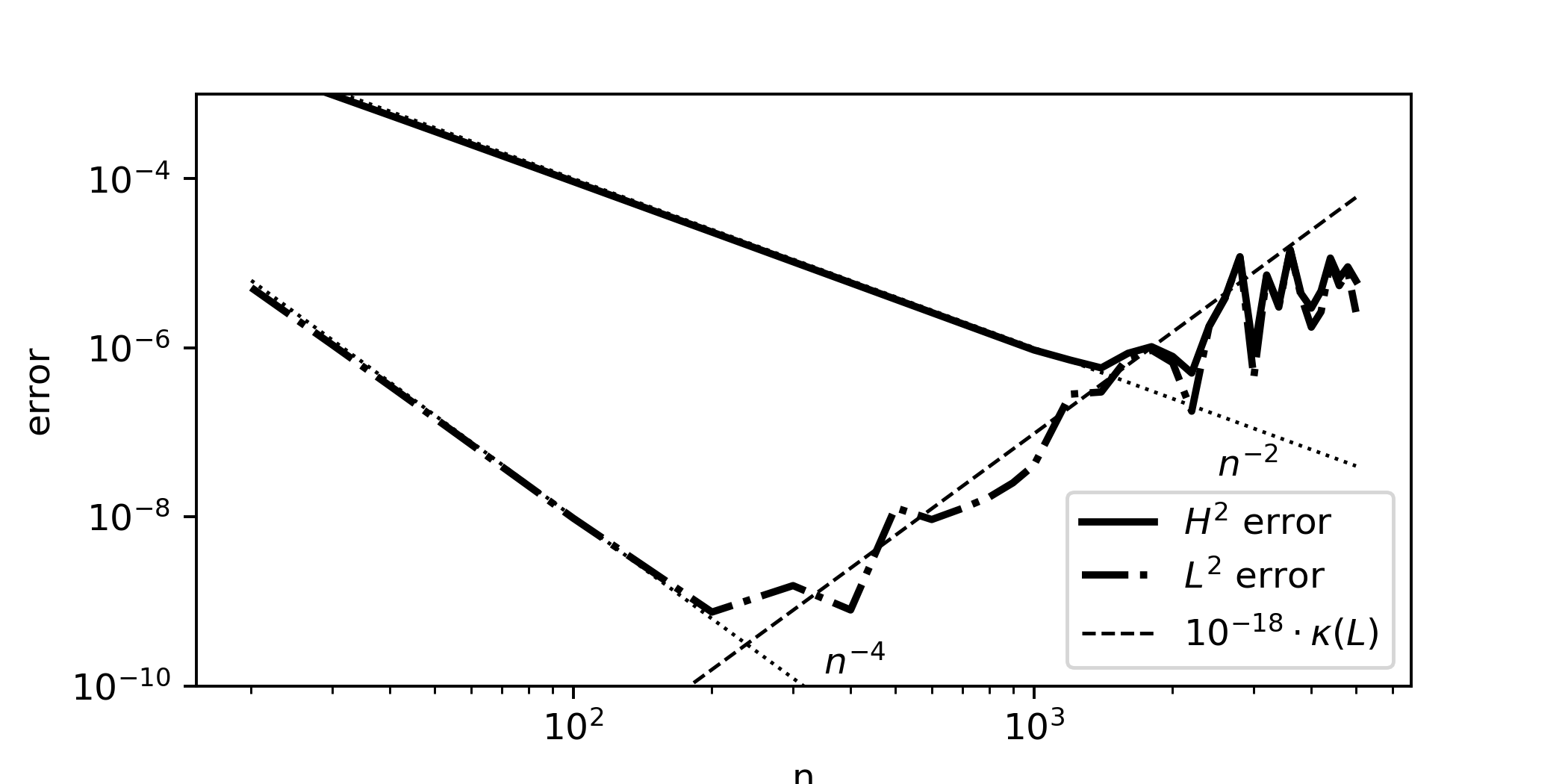
Figure 5.1: Relative error $\|u-\hat{u}\|/\|u\|$ as a function of the number of cells $n$ of the finite-element approximation $\hat{u}$ to the true solution $u=(1-x^{2})^{2}$ of the biharmonic equation with constant right-hand side $u^{(4)}(x)=24$. The solution is approximated with Hermite elements, and error is computed in $H^{2}$ and $L^{2}$ norms. Integrals were computed using Gaussian quadrature with $11$ quadrature points per cell. Also shown are the expected $\mathcal{O}(n^{-2})$-scaling of the error and the multiple $\epsilon\kappa(\mathbf{L})$ of the involved matrix, where $\epsilon=10^{-18}$ is close to machine precision.

5.2 Integration preconditioning for fourth-order differential equations

Consider now an operator $\mathcal{R}$ to be used as a right preconditioner for the differential equation $\mathcal{L}u=f$. Replacing $u$ by $\mathcal{R}v$, where $v$ is any function that is mapped by $\mathcal{R}$ to the same smoothness and boundary properties as $u$,

$$\mathcal{R}v\in H_{0}^{2}(-1,1),$$ (5.3)

we find for $w\in H^{2}_{0}(-1,1)$ that $\mathcal{R}v$ may also replace $u$ in the bilinear form $\mathsf{a}(w,\mathcal{R}v)$.

The system matrix for the preconditioned operator equation is again obtained by computing the bilinear form on all $2n\times 2n$ pairs of Hermite basis functions and is given by its entries

$$\tilde{\mathbf{L}}[j,k]=\mathsf{a}(\phi_{j},\mathcal{R}\phi_{k}).$$

Notably, the knowledge of $\mathsf{a}(\cdot,\mathcal{R}\cdot)$ for arbitrary arguments is not required. Instead, for the computation of the matrix evaluation of the preconditioner on the elements $\phi_{k}$ of the Hermite basis and computation of $\mathsf{a}$ on pairs of $\phi_{j}$ and $\mathcal{R}\phi_{k}$ is sufficient.

For a fourth-order differential operator with leading-order term $\frac{d^{4}}{dx^{4}}$, we use four-fold integration as the preconditioner. Moreover, for $\mathcal{L}:H^{2}_{0}(-1,1)\to H^{-2}(-1,1)$, the four-fold integration preconditioner is chosen such that it takes care of boundary conditions, i.e. $\mathcal{R}:H^{2}_{0}(-1,1)\to H^{-2}(-1,1)$.

Computing $\Phi_{k}=\mathcal{R}\phi_{k}$ for $k\in\{1,\dotsc,2n\}$ is straightforward. During the cell-wise integration of $\phi_{k}$, $k\in\{1,\dotsc,2n\}$, in each of the $n+1$ cells, $4$ degrees of freedom arise in the form of integration constants. The first $4n$ of these are chosen such that $\Phi_{k}$ and its first three derivatives are continuous on the boundaries between the cells. Because $\phi_{k}$ is continuous with continuous first derivative, it follows that $\Phi_{k}\in H^{2}(-1,1)$. The last four integration constants are determined by the boundary conditions of $H^{2}_{0}(-1,1)$. Hence, $\Phi_{k}\in H^{2}_{0}(-1,1)$ is guaranteed.

The resulting functions $\Phi_{k}=\mathcal{R}\phi_{k}$ are used as the trial-space basis. The matrix $\tilde{\mathbf{L}}$ is computed numerically using Gaussian quadrature. After solving the system $\tilde{\mathbf{L}}\mathbf{v}=\mathbf{b}$, we reconstruct the solution $\hat{u}=\sum_{k=1}^{2n}v_{k}\Phi_{k}$.

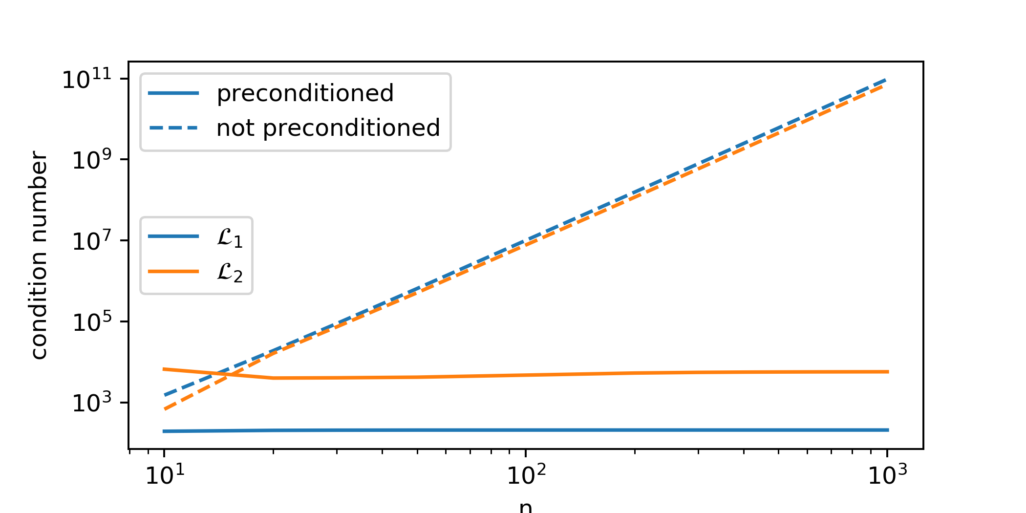
Figure 5.2: Condition numbers of the non-preconditioned and preconditioned method for the biharmonic equation $\mathcal{L}_{1}$ and the differential operator $\mathcal{L}_{2}$ defined in equation (5.5)

Instead of growing as $\mathcal{O}(n^{4})$, the condition number of $\tilde{\mathbf{L}}$ approaches a constant as $n\to\infty$. Figure 5.2 shows the condition number of the matrices $\mathbf{L}$ and $\tilde{\mathbf{L}}$ for the biharmonic equation

$$\mathcal{L}_{1}=\frac{d^{4}}{dx^{4}}u$$ (5.4)

and for the equation with operator

$$\mathcal{L}_{2}=\frac{d^{4}}{dx^{4}}+\alpha\sin(20\pi x)\frac{d^{3}}{dx^{3}}+\alpha\cos(20\pi x^{3})\frac{d^{2}}{dx^{2}}+\frac{\alpha x}{1+x^{2}}$$ (5.5)

with $\alpha=200$. We see that up to $n=1000$, the condition number of the preconditioned matrices does not increase beyond $~{}100$ and $10000$, respectively, whereas condition numbers obtained from the standard algorithm show a clear $\mathcal{O}(n^{4})$ growth.

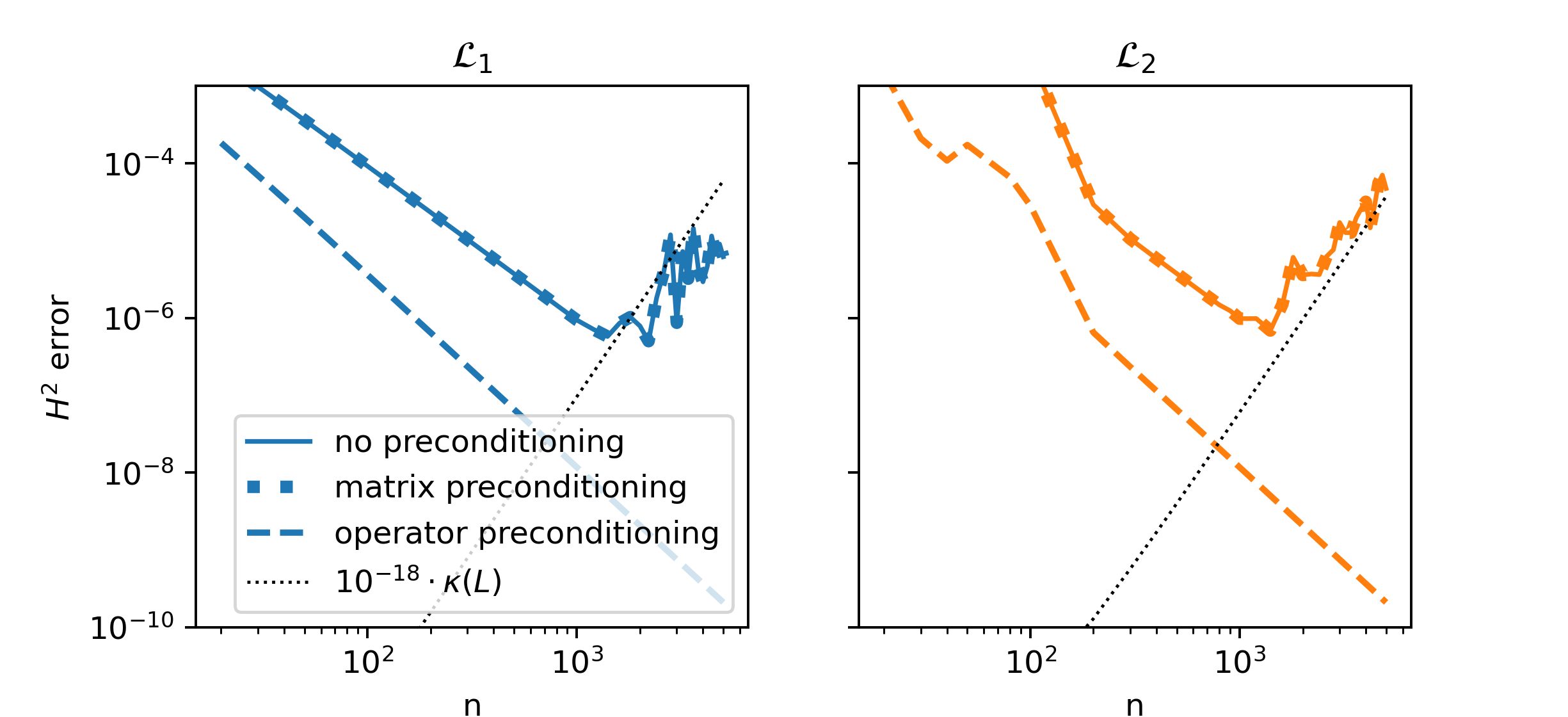
Figure 5.3: Relative error of the approximation to the solution $u=(1-x^{2})^{2}$ obtained with non-preconditioned, matrix-preconditioned with the inverse of the stiffness matrix of the biharmonic equation, and operator-preconditioned Hermite FEM for the two differential equations with differential operators $\mathcal{L}_{1}$ and $\mathcal{L}_{2}$ defined in equations (5.4) and (5.5). Note that matrix preconditioning and the unpreconditioned method lead to the same relative error.

Accordingly, solutions obtained from the preconditioned method do not suffer from an erratic increase of error for high $n$ as in Figure 5.1. A comparison is shown in Figure 5.3. As before, for the nonpreconditioned method, the error starts to increase once $\epsilon\kappa(\mathbf{L})$ grows to the range of the discretization error and it remains above $10^{-7}$ for all $n$. The same holds for matrix preconditioning: The matrix equivalent of four-fold differentiation is the finite-element discretization of the biharmonic operator $\frac{d^{4}}{dx^{4}}$. Using the inverse of this matrix as a preconditioner leads to no visible changes in the relative error. On the other hand, FOP is able to find solutions to the problem with error as low as $10^{-10}$ at $n=5000$, and with no deviations from the trend of decreasing error when $n$ is increased.

This accuracy is possible because the condition number of the FOP system matrix $\tilde{\mathbf{L}}$ remains bounded. As we shall see, this is a consequence of two conditions:

$i)$ the operator $\tilde{\mathcal{L}}:=\mathcal{L}\mathcal{R}$ is an endomorphism in $H^{-2}(-1,1)$ [11, 32].

Indeed, this condition allows us to state the following: Let $\mathsf{\tilde{b}}(\cdot,\cdot):H^{-2}(-1,1)\times H^{-2}(-1,1)\to\mathbb{R}$ be the bilinear form of $\tilde{\mathcal{L}}$. By the properties of $\mathcal{L}$ and $\mathcal{R}$, there exist constants $\tilde{\beta},\tilde{C}_{b}\in\mathbb{R}>0$ such that

$$\tilde{\beta}\,\|u\|_{H^{-2}(-1,1)}^{2}\leq|\mathsf{\tilde{b}}(u,u)|\leq\tilde{C}_{b}\,\|u\|_{H^{-2}(-1,1)}^{2}\qquad\forall u\in H^{-2}(-1,1).$$ (5.6)

It is worth noticing that using $\mathcal{R}$ as a left preconditioner would also lead to a suitable FOP. Indeed, in that case we would have the endomorphism $\widehat{\mathcal{L}}:=\mathcal{R}\mathcal{L}:H^{2}_{0}(-1,1)\to H^{2}_{0}(-1,1)$, satisfying for some $\widehat{\beta},\widehat{C}_{b}>0$

$$\widehat{\beta}\,\|u\|_{H^{2}_{0}(-1,1)}^{2}\leq|\mathsf{\widehat{b}}(u,u)|\leq\widehat{C}_{b}\,\|u\|_{H^{2}_{0}(-1,1)}^{2}\qquad\forall u\in H^{2}_{0}(-1,1).$$ (5.7)

$ii)$ The Hermite basis functions are well-conditioned.

In order to see this, we examine the mass matrix

$$\mathbf{M}[j,k]=(\phi_{j},\phi_{k})_{L^{2}(-1,1)}.$$ (5.8)

Recalling the definition and support of the Hermite functions [9, § 3.2], integration yields the structure of the mass matrix

$$\mathbf{M}=\Delta x\begin{pmatrix}\mathbf{A}&\mathbf{B}&&\\ \mathbf{B}^{\top}&\mathbf{A}&\mathbf{B}&\\ &\mathbf{B}^{\top}&\mathbf{A}&\mathbf{B}\\ &&\ddots&\ddots\end{pmatrix}\in\mathbb{R}^{2n\times 2n}$$ (5.9)

with the $2\times 2$ blocks

$$\mathbf{A} =\begin{pmatrix}26/35&0\\ 0&2/105\end{pmatrix}, \qquad\mathbf{B}=\begin{pmatrix}9/70&13/420\\ -13/420&-1/140\end{pmatrix}.$$

Proposition 5.1.

For all $n\in\mathbb{N}$, the matrix $\mathbf{M}$ in (5.9) satisfies

$$\kappa(\mathbf{M})\leq 39\frac{1+\delta}{1-\delta},\qquad\delta=\frac{3+\sqrt{13/3}}{8}\ (<0.64).$$

Proof.

The idea is to use Gerschgorin’s theorem to a diagonally scaled matrix $\tilde{\mathbf{M}}:=\mathbf{D}\mathbf{M}\mathbf{D}$, where $\mathbf{D}=\mbox{diag}(\mathbf{D}_{1},\mathbf{D}_{1},\ldots)\in\mathbb{R}^{2n\times 2n}$, with $\mathbf{D}_{1}=\big{(}\begin{smallmatrix}\sqrt{35/26}&0\\ 0&\sqrt{105/2}\end{smallmatrix}\big{)}$; that is, we apply a diagonal scaling such that $\mathbf{D}\mathbf{M}\mathbf{D}$ has 1’s on the diagonal.

Then $\tilde{\mathbf{M}}$ is in the same form as $\mathbf{M}$ (5.9), with $\mathbf{A},\mathbf{B}$ replaced with $\tilde{\mathbf{A}},\tilde{\mathbf{B}}$ respectively, where

$$\tilde{\mathbf{A}} =\begin{pmatrix}1&0\\ 0&1\end{pmatrix}, \qquad\tilde{\mathbf{B}}=\begin{pmatrix}9/52&\sqrt{13}/(8\sqrt{3})\\ -\sqrt{13}/(8\sqrt{3})&-3/8\end{pmatrix}.$$

Now by Gerschgorin’s theorem, (and since $\tilde{\mathbf{M}}$ is symmetric) the eigenvalues of $\tilde{\mathbf{M}}$ must lie in $[1-\frac{1}{8}(3+\sqrt{13/3}),1+\frac{1}{8}(3+\sqrt{13/3})]=[1-\delta,1+\delta]$. Since this is a positive interval, it follows that $\tilde{\mathbf{M}}$ is positive definite and the eigenvalues are equal to the singular values. Therefore $\kappa(\tilde{\mathbf{M}})\leq\frac{1+\delta}{1-\delta}$. Finally, $\kappa(\mathbf{M})\leq\kappa(\tilde{\mathbf{M}})\kappa(\mathbf{D})^{2}$ and $\kappa(\mathbf{D})^{2}=\kappa(\mathbf{D}_{1})^{2}=39$, completing the proof. ∎

Next, we proceed to prove in a more general way why these two conditions guarantee that we arrive at a well-conditioned system.

Theorem 5.2.

Let $X$ be a Hilbert space, and $\mathsf{b}$ a bounded bilinear form $\mathsf{b}(\cdot,\cdot):X\times X\to\mathbb{R}$ so that there exists $M>0$ such that $|\mathsf{{b}}(v,u)|\leq M\|u\|_{X}\|v\|_{X}$ for all $v\in X$. Suppose that $\mathsf{b}$ further satisfies

$${\beta}\,\|u\|_{X}^{2}\leq|\mathsf{{b}}(u,u)|\qquad\forall v\in X,$$ (5.10)

for some $\beta>0$.

Let $X_{h}\subset X$ be a finite dimensional space such that $\mathsf{dim}(X_{h})=N$ and $X_{h}=\mathsf{span}\{q_{i}\}_{i=1}^{N}$. Then the matrix $\mathbf{B}_{h}$ defined by $(\mathbf{B}_{h})_{ij}=\mathsf{b}(q_{j},q_{i})$ satisfies

$$\kappa(\mathbf{B}_{h})\leq\frac{M}{\beta}(\kappa(\mathcal{Q}))^{2},$$ (5.11)

where $\mathcal{Q}=[q_{1},\ldots,q_{N}]$ is a quasimatrix, i.e., a matrix whose columns are functions (e.g. [16]).

Proof.

First, let $B\in L(X,X)$ be the bounded linear mapping corresponding to the bilinear form $\mathsf{b}$.

For any $\mathbf{u}=(u_{1},\ldots,u_{N})^{\top},\mathbf{v}=(v_{1},\ldots,v_{N})^{\top}\in\mathbb{C}^{N}$ of unit norm $\|\mathbf{u}\|_{2}=\|\\ mathbf{v}\|_{2}=1$, we have

$$(\mathbf{B}_{h}\mathbf{v})[j]=\mathsf{b}(q_{j},\sum_{\ell=1}^{N}v_{\ell}q_{\ell}),\qquad\mathbf{u}^{\top}\mathbf{B}_{h}\mathbf{v}=\mathsf{b}(\sum_{\ell=1}^{N}u_{\ell}q_{j},\sum_{\ell=1}^{N}v_{\ell}q_{\ell}).$$

Hence by the assumption (5.10) we have

$$\beta\|\sum_{\ell=1}^{N}v_{\ell}q_{\ell}\|_{X}^{2}\leq|\mathbf{v}^{\top}\mathbf{B}_{h}\mathbf{v}|.$$ (5.12)

We can bound $\|\sum_{\ell=1}^{N}v_{\ell}q_{\ell}\|_{X}$ as

$$\sigma_{\min}(\mathcal{Q})\leq\|\sum_{\ell=1}^{N}v_{\ell}q_{\ell}\|_{X}\leq\sigma_{\max}(\mathcal{Q}).$$ (5.13)

It follows that $|\mathbf{v}^{\top}\mathbf{B}_{h}\mathbf{v}|\geq\sigma_{\min}^{2}(\mathcal{Q})\beta$ for any unit vector $\mathbf{v}$; this implies $\|\mathbf{B}_{h}\mathbf{v}\|_{2}\geq\sigma_{\min}^{2}(\mathcal{Q})\beta$ for any unit norm vector $\mathbf{v}$, and therefore $\sigma_{\min}(\mathbf{B}_{h})\geq\sigma_{\min}^{2}(\mathcal{Q})\beta$.

We next bound $\sigma_{\max}(\mathbf{B}_{h})=\|\mathbf{B}_{h}\|_{2}$ from above. The first bound in (5.10) and (5.11) yield $|\mathbf{u}^{\top}\mathbf{B}_{h}\mathbf{v}|\leq M\sigma_{\max}^{2}(\mathcal{Q})$, for any $\mathbf{u},\mathbf{v}$ of unit norm. This means $\mathbf{B}_{h}\leq M\sigma_{\max}^{2}(\mathcal{Q})$.

Putting these together, we conclude that

$$\kappa(\mathbf{B}_{h})\leq\frac{M\sigma_{\max}^{2}(\mathcal{Q})}{\sigma_{\min}^{2}(\mathcal{Q})\beta}=\frac{M}{\beta}(\kappa(\mathcal{Q}))^{2}.$$

∎

This result shows that the linear system is well-conditioned if the operator after FOP has a tightly bounded bilinear form, and a well-conditioned basis $\mathcal{Q}$ is used for the discretization, ideally $\kappa(\mathcal{Q})$ not growing with the discretization $N$.

It is worth noting that the presence of $(\kappa(\mathcal{Q}))^{2}$ in (5.16) appears to be necessary, and is not an artifact of the analysis. To see this, consider the case $\mathcal{L}\mathcal{R}=\mathcal{I}$ (the ’ideal FOP’); then $\tilde{\mathbf{L}}_{h}$ is the Gram matrix of $\mathcal{Q}$, so $\kappa(\tilde{\mathbf{L}}_{h})=(\kappa(\mathcal{Q}))^{2}$.

Let us now return to the specific examples in Figure 5.3. Since the mass matrix (5.8) has the property $\kappa(\mathbf{M})=(\kappa(\mathcal{Q}))^{2}$. Theorem 5.2 and Proposition 5.1 imply that $\kappa(\tilde{\mathbf{L}}_{1h})$ is bounded independently of $n$ for (5.4), for which $\beta=M=1$.

5.3 Perturbed identity after FOP

In many cases, such as (5.5), the operator after FOP is a perturbed identity $\mathcal{I}+\mathcal{K}$. In such cases we have the following.

Corollary 5.3.

Let $\mathcal{R}$ be such that

$$\mathcal{L}\mathcal{R}=\mathcal{I}+\mathcal{K}:X\to X,$$ (5.14)

where $\mathcal{I}$ is the identity operator, and $\mathcal{K}$ is bounded, i.e., there exists $M_{\mathcal{K}}>0$ such that $(u,\mathcal{K}u)_{X}\leq M_{\mathcal{K}}\|u\|_{X}\|v\|_{X}$ for all $u,v\in X$. Suppose that

$$\beta_{\mathcal{K}}\|u\|_{X}^{2}\leq(u,\mathcal{K}u)_{X}\qquad\forall u\in X,$$ (5.15)

for some constant $\beta_{\mathcal{K}}>-1$. Then we have

$$\kappa(\tilde{\mathbf{L}}_{h})\leq\frac{1+M_{\mathcal{K}}}{1+\beta_{\mathcal{K}}}(\kappa(\mathcal{Q}))^{2}$$ (5.16)

where $\tilde{\mathbf{L}}_{h}$ is the Galerkin matrix of $\tilde{\mathcal{L}}:=\mathcal{L}\mathcal{R}$ using the basis functions $\{q_{i}\}_{i=1}^{N}$, and $\mathcal{Q}=[q_{1},\ldots,q_{N}]$.

Proof.

By the assumptions, we have

$$(1+\beta_{\mathcal{K}})\|u\|_{X}^{2} \leq(u,(\mathcal{I}+\mathcal{K})u)_{X}, (v,(\mathcal{I}+\mathcal{K})u)_{X}\leq(1+M_{\mathcal{K}})\|u\|_{X}\|v\|_{X}$$ (5.17)

for all $u,v\in X$. Therefore, the result follows from Theorem 5.2. ∎

Remark 5.4.

Theorem 5.3 indicates that two conditions ensure $\tilde{\mathbf{L}}_{h}$ is well-conditioned: (i) that the FOP is effective so that the FOP’d operator is a “small” perturbation of identity, and (ii) a well-conditioned basis $\mathcal{Q}$ is chosen. We suspect that the assumptions in Corollary 5.3 are stronger than necessary, and that $\kappa(\tilde{\mathbf{L}}_{h})$ could be bounded by a constant under a looser condition than (5.15).

Remark 5.5.

A good FOP often results in the form (5.14) with a compact $\mathcal{K}$. For instance, in the example (5.5), under the assumption of continuously differentiable coefficient functions and by compactness of the embeddings $H^{\lambda+1}(-1,1)\subset H^{\lambda}(-1,1)$ for $\lambda\geq 0$ [28, Chapter 1], we have $\mathcal{L}\mathcal{R}=\mathcal{I}+\mathcal{K},$ where

$$\mathcal{K}=\left(a_{3}\frac{d^{3}}{dx^{3}}+a_{2}\frac{d^{2}}{dx^{2}}+a_{1}\frac{d^{1}}{dx^{1}}+a_{0}\right)\mathcal{R}$$

is a compact operator.

The “identity plus compact operator” resembles the situation in Section 4.2. Compactness of $\mathcal{K}$ can be useful for verifying its properties, such as (5.15).

Furthermore, the extension to $\mathcal{L}\mathcal{R}=\mathcal{I}+\mathcal{K}$ highlights another specialty of FOP: When investigating the properties of any form of preconditioning, we aim for statements about the resulting matrices. Analysis of matrix-preconditioning schemes may take place on the matrix level, for example by bounding the generalized Rayleigh coefficient $(\mathbf{u}^{\top}\mathbf{L}\mathbf{u})/(\mathbf{u}\mathbf{R}^{-1}\mathbf{u})$ [47]. This is also possible when all elements and operators on the continuous space have representations in terms of infinite-dimensional matrices, such as in the case of spectral methods. For other cases of FOP, however, another option is to perform analysis on the levels of the operators themselves. This diffuses the classical distinction between numerical linear algebra and analysis of differential equations and calls for joint treatment of the whole solution process, a claim that is already being pushed for by other authors such as [38] and [41].

6 Discussion

FOP can dramatically improve the accuracy of computed solutions in a variety of contexts. Our analysis identifies three properties required for a successful FOP. First, one needs to identify an operator such that its composition with $\mathcal{L}$ is an endomorphism. Second, the test and trial basis must be chosen to be conforming and well-conditioned. With these two properties, one can guarantee that the condition number remains bounded. Third, after FOP is applied, the matrix and right-hand side in the linear system need to be computed with high accuracy. As discussed in Section 5, this can be guaranteed by requiring that the preconditioned operator $\tilde{\mathcal{L}}$ is continuous.

We have highlighted two classical applications (polynomial interpolation and spectral methods) that can be regarded as an instance of FOP. We believe that many other high-accuracy algorithms (existing and forthcoming) could also be understood as a form of FOP, and that much can be learned by revisiting existing methods and establishing connections from this perspective.

It is important to point out the potential drawbacks of FOP. First, some desirable structures in the unpreconditioned system may be lost. For example, the FOP in Section 5 results in dense matrices. This negates the sparsity of the unpreconditioned system, one of the typical benefits of FEM. Another drawback is the difficulty of finding a good FOP, that is, identifying an operator verifying the first property listed above. Fortunately, this is also needed in operator preconditioning [32]. Therefore, investigations of such operators have already taken place in the literature, see for example [47, 26, 27, 20] and the references therein. Building on this well-established knowledge about operator preconditioning, it remains to come up with a suitable discretization.

For many applications of scientific computing, this is an open challenge. By overcoming it, one would obtain solutions with unprecedented accuracy.

References

- [1] Ahmad Abdelfattah, Hartwig Anzt, Erik G Boman, Erin Carson, Terry Cojean, Jack Dongarra, Mark Gates, Thomas Grützmacher, Nicholas J Higham, Sherry Li, et al. A survey of numerical methods utilizing mixed precision arithmetic. arXiv preprint arXiv:2007.06674, 2020.
- [2] Kendall E Atkinson. An Introduction to Numerical Analysis. Wiley, New York ; Chichester, 2nd edition, 1989.
- [3] O. Axelsson and J. Karátson. Equivalent operator preconditioning for elliptic problems. Numer. Algorithms, 50(3):297–380, 2009.
- [4] Randolph E. Bank and L. Ridgway Scott. On the conditioning of finite element equations with highly refined meshes. SIAM J. Numer. Anal., 26(6):1383–1394, 1989.
- [5] Bernhard Beckermann. The condition number of real Vandermonde, Krylov and positive definite Hankel matrices. Numer. Math., 85(4):553–577, 2000.
- [6] Timo Betcke and Lloyd N. Trefethen. Reviving the method of particular solutions. SIAM Rev., 47(3):469–491, 2005.
- [7] Daniele Boffi, Franco Brezzi, and Michel Fortin. Mixed Finite Element Methods and Applications, volume 44. Springer, 2013.
- [8] John P Boyd. Chebyshev and Fourier Spectral Methods. Dover Publications, Mineola, N.Y., 2nd edition, 2001.
- [9] Susanne Brenner and Ridgway Scott. The Mathematical Theory of Finite Element Methods, volume 15. Springer Science & Business Media, 2007.
- [10] C. Canuto, M. Yousuff Hussaini, Alfio Quarteroni, and Thomas A. Zang. Spectral methods : fundamentals in single domains. Scientific computation. Springer, Berlin, 2010.
- [11] Snorre H. Christiansen. Résolution des équations intégrales pour la diffraction d’ondes acoustiques et électromagnétiques - Stabilisation d’algorithmes itératifs et aspects de l’analyse numérique. Theses, Ecole Polytechnique X, January 2002.
- [12] Philippe G. Ciarlet. The Finite Element Method for Elliptic Problems. SIAM, 2002.
- [13] C. W. Clenshaw. The numerical solution of linear differential equations in chebyshev series. Mathematical Proceedings of the Cambridge Philosophical Society, 53(1):134–149, 1957.
- [14] E. A. Coutsias, T. Hagstrom, J. S. Hesthaven, and D. Torres. Integration preconditioners for differential operators in spectral -methods. In Proceedings of the Third International Conference on Spectral and High Order Methods, Houston, TX, pages 21–38, 1996.
- [15] Evangelos A. Coutsias, Thomas Hagstrom, and David Torres. An efficient spectral method for ordinary differential equations with rational function coefficients. Math. Comp., 65(214):611–635, 1996.
- [16] T. A. Driscoll, N. Hale, and L. N. Trefethen. Chebfun Guide. Pafnuty Publications, Oxford, 2014.
- [17] Elsayed M. E. Elbarbary. Integration preconditioning matrix for ultraspherical pseudospectral operators. SIAM J. Sci. Comp, 28(3):1186–1201, 2006.
- [18] Patrick. E. Farrell. Finite element methods for pdes. Oxford University lecture notes, 2020.
- [19] Walter Gautschi. Norm estimates for inverses of vandermonde matrices. Numer. Math., 23(4):337–347, 1974.
- [20] Heiko Gimperlein, Jakub Stocek, and Carolina Urzúa-Torres. Optimal operator preconditioning for pseudodifferential boundary problems. Numer. Math., 2021.
- [21] Philippe Grandclement. Introduction to spectral methods. EAS Publ. Ser., 21:153–180, 2006.
- [22] Anne Greenbaum. Iterative Methods for Solving Linear Systems. SIAM, 1997.
- [23] Anne Greenbaum, Vlastimil Ptak, and Zdenve K Strakos. Any nonincreasing convergence curve is possible for GMRES. SIAM J. Matrix Anal. Appl., 17(3):465, 1996.
- [24] Leslie Greengard. Spectral integration and two-point boundary value problems. SIAM J. Numer. Anal., 28(4):1071–1080, 1991.
- [25] Leslie Greengard and Vladimir Rokhlin. On the numerical solution of two-point boundary value problems. Comm. Pure Appl. Math., 44(4):419–452, 1991.
- [26] Chen Greif and Dominik Schötzau. Preconditioners for saddle point linear systems with highly singular blocks. Electron. Trans. Numer. Anal., 22:114–121, 2006.
- [27] Chen Greif and Dominik Schötzau. Preconditioners for the discretized time-harmonic Maxwell equations in mixed form. Numer. Lin. Alg. Appl., 14(4):281–297, 2007.
- [28] Pierre Grisvard. Elliptic Problems in Nonsmooth Domains. SIAM, 2011.
- [29] W. Hackbusch. Iterative solution of large sparse systems of equations. Applied Mathematical Sciences; 95. Springer, Switzerland, 2nd edition, 2016.
- [30] W. Hackbusch, Regine Fadiman, and Patrick D. F Ion. Elliptic differential equations : theory and numerical treatment. Springer series in computational mathematics; 18. Springer-Verlag, Berlin ; London, 1992.
- [31] Nicholas J. Higham. Accuracy and Stability of Numerical Algorithms. SIAM, second edition, 2002.
- [32] R. Hiptmair. Operator preconditioning. Comput. Math. with Appl., 52(5):699 – 706, 2006.
- [33] Randall J LeVeque. Finite difference methods for ordinary and partial differential equations: steady-state and time-dependent problems. SIAM, 2007.
- [34] Jörg Liesen and Petr Tichý. Convergence analysis of Krylov subspace methods. GAMM‐Mitteilungen, 27(2):153–173, 2004.
- [35] Kent-Andre Mardal and Ragnar Winther. Preconditioning discretizations of systems of partial differential equations. Numer. Lin. Alg. Appl., 18(1):1–40, 2011.
- [36] Vladimir Maz’ya. Continuity and Boundedness of Functions in Sobolev Spaces, pages 405–434. Springer Berlin Heidelberg, Berlin, Heidelberg, 2011.
- [37] Stephan Mohr. Full operator preconditioning and the accuracy of solving linear systems. Master’s thesis, University of Oxford, 2020.
- [38] Josef Málek and Zdeněk Strakoš. Preconditioning and the Conjugate Gradient Method in the Context of Solving PDEs. SIAM, Philadelphia, PA, 2014.
- [39] Sheehan Olver and Alex Townsend. A fast and well-conditioned spectral method. SIAM Rev., 55(3):462–489, 2013.
- [40] Werner Rmisch and Thomas Zeugmann. Mathematical Analysis and the Mathematics of Computation. Springer Publishing Company, Incorporated, 1st edition, 2016.
- [41] Yousef Saad. Iterative Methods for Sparse Linear Systems. SIAM, 2003.
- [42] Josef Stoer and Roland Bulirsch. Introduction to Numerical Analysis. Texts in Applied Mathematics; 12. Springer-Verlag, New York; London, 2nd ed. edition, 1993.
- [43] Gilbert Strang. The discrete cosine transform. SIAM Rev., 41(1):135–147, 1999.
- [44] Lloyd N. Trefethen. Spectral Methods in MATLAB. SIAM, 2000.
- [45] Lloyd N. Trefethen. Householder triangularization of a quasimatrix. IMA J. Numer. Anal., 30(4):887–897, 2010.
- [46] Lloyd N Trefethen. Approximation Theory and Approximation Practice. SIAM, Philadelphia, 2013.
- [47] Andrew Wathen. Preconditioning. Acta Numerica, 24, 2015.