ADMM and Spectral Proximity Operators in Hyperspectral Broadband Phase Retrieval for Quantitative Phase Imaging

Abstract

A novel formulation of the hyperspectral broadband phase retrieval is developed for the scenario where both object and modulation phase masks are spectrally varying. The proposed algorithm is based on a complex domain version of the alternating direction method of multipliers (ADMM) and Spectral Proximity Operators (SPO) derived for Gaussian and Poissonian observations. Computations for these operators are reduced to the solution of sets of cubic (for Gaussian) and quadratic (for Poissonian) algebraic equations. These proximity operators resolve two problems. Firstly, the complex domain spectral components of signals are extracted from the total intensity observations calculated as sums of the signal spectral intensities. In this way, the spectral analysis of the total intensities is achieved. Secondly, the noisy observations are filtered, compromising noisy intensity observations and their predicted counterparts. The ability to resolve the hyperspectral broadband phase retrieval problem and to find the spectrum varying object are essentially defined by the spectral properties of object and image formation operators. The simulation tests demonstrate that the phase retrieval in this formulation can be successfully resolved.

1 Introduction

Multispectral (MS) and hyperspectral (HS) images differ in amount and width of spectral channels. The number of spectral channels varies from a few to tens for MS images and goes from tens up to hundreds for HS images. We do not make a difference between these two scenarios and use the word ’hyperspectral’ addressing to both MS and HS ones. The HS imaging is much more informative as compared with the conventional RGB imaging and indispensable in many applications such as remote sensing, biology, medicine, quality material and food characterization, control of ocean and earth pollution, etc.  A flow of publications on computational methods developed for various applications of HS imaging is growing fast (e.g. [1, 2, 3]).

A spectral information is provided by optical devices (spectrometers) or in numerical form by computational methods in two different modes: (1) registered and processed channel-by-channel or (2) registered as the total power of entire spectral channels with a subsequent spectral analysis. In this paper, we consider the latter scenario with a broadband illumination of an object of interest and a broadband sensor registering the total power of the impinging light beam.

The HS phase imaging is a comparatively new development dealing with a phase delay of a coherent light in transparent or reflective objects [4, 5]. The HS broadband phase imaging is more informative than the monochromatic one and provides more precise information and visualization of invisible. It is one of the most promising directions in quantitative phase imaging [6, 7, 8, 9] with numerous applications in optical metrology [10], microscopy [11], digital holography[12], biology and medicine[13]. In particular, the quantitative phase imaging enables label-free and quantitative assessment of cells and tissues, which plays an important role in study of their optical, chemical, and mechanical intrinsic properties [14, 15, 16, 17].

Contrary to the intensity imaging, the phase imaging is more complex as the quantitative phase cannot be measured directly and should be extracted from the indirect intensity observations. The conventional phase imaging employing the principles of interferometry exploits the reference beams, and the interference between the object and the reference beams is a source of the phase information for the object.

Conventionally, for the processing of HS images, 2D spectral narrow-band images are stacked together and represented as 3D cubes with two spatial coordinates $(x,y)$ and the third longitudinal spectral coordinate. In phase imaging, data in these 3D cubes are complex-valued with spatial and spectral varying amplitudes and phases. Due to this, phase image processing is more complex than the HS intensity imaging where the corresponding 3D cubes are real-valued.

The usual setup of monochromatic phase retrieval assumes recovering of a complex-valued object $U_{o}\in\mathbb{C}^{N}$ from multiple (or single) intensity measurements (squared linear projections) $Y_{t}=|A_{t}U_{o}|^{2},$ $t=1,...,T$, where $Y_{t}\in\mathbb{R}^{M}$, and $A_{t}\in\mathbb{C}^{M\times N}$ is an image formation operator. The heuristic iterative algorithms with alternative projections to the object and measurement planes are well known and studied starting from the works of Gerchberg and Saxton [18] and Fienup [19]. These techniques are proven to be efficient for various optical applications.

The common setup for phase retrieval assumes a modulation of the object $U_{o}$ by the random phase mask $\mathcal{M}_{t}\in\mathbb{C}^{N}$ with the observation model

$$Y_{t}=|A_{t}(\mathcal{M}_{t}\circ U_{o})|^{2},\text{ }t=1,...,T,$$ (1)

where ’$\circ$’ stands for the Hadamard, element-by-element, product of two vectors.

In general, the phase retrieval is a non-convex inverse imaging problem. Theoretical studies formulating restrictions on object and image formation models leading to uniqueness and convergence of the iterative algorithms are of special interest. The model (1) with the operator $A_{t}$ given as the Fourier transform (FT) is common for many theoretical works [20], [21], [22]. Optimization of the phase coding modulation masks $\mathcal{M}_{t}$ is a hot topics in phase retrieval [8], [23], [24]. The extended review of the recent developments in mathematical foundation of the phase retrieval problems can be seen in [25], [26], [27].

In this paper, we propose a novel phase retrieval formulation providing a prospective powerful instrumentation for broadband HS complex domain (phase/amplitude) imaging. In what follows we use the convenient vectorized representation of $2D$ images as vectors. For the object of interest it is the vector $U_{o,k}\in\mathbb{C}^{N}$, $N=nm$, where $n$ and $m$ are width and height of $2D$ image; $k$ stays for the spectral variable, which is a wavenumber in optics, $k=\dfrac{2\pi}{\lambda}$, $\lambda$ is a wavelength.

We introduce the HS broadband phase retrieval as a reconstruction of the complex-valued object $U_{o,k}\in\mathbb{C}^{N},$ $k\in K$, from the intensity measurements:

$$Y_{t}=\sum_{k\in K}|A_{t,k}U_{o,k}|^{2},\text{ }t\in T.$$ (2)

For the noisy intensity observations with additive noise $\varepsilon_{t}$, $Y_{t}$ is replaced by $Z_{t}$:

$$Z_{t}=Y_{t}+\varepsilon_{t},~{}t\in T.$$ (3)

Here $A_{t,k}\in\mathbb{C}^{M\times N}$ are linear operators modeling  a propagation of 2D object images from the object plane to the sensor,  and $t$ is the index of experiment. The total intensity measurements $Y_{t}\in R_{+}^{M}$ are calculated over the spectrum $K$ as the sum of the spectral intensities $|A_{t,k}U_{o,k}|^{2}$. It is essential in this paper, that the object $U_{o,k}$ and the operators $A_{t,k}$ are spectrum dependent, varying in $k$. In optics, it means that the reflective and transmissive properties of the object (specimen) as well as the light propagation operators depend on the wavelength of light.

There is a small number of publications relevant to the HS broadband phase retrieval from the total intensity measurements considered in this paper. We briefly review these works.

The HS phase retrieval in the paper [28] is formulated as object reconstruction from the intensity observations $Y_{t}=\sum_{k\in K}|A_{t,k}U_{o}|^{2}$, where the object $U_{o}$ is spectrally invariant, i.e. does not depends on $k$. This assumption differs [28] essentially from the setup considered in this paper.

With the introduced observation model (2), the interferometric HS methods also can be interpreted as the phase retrieval problems. Indeed, the HS digital holography uses the observation model

$$Y_{t}=\sum_{k\in K}|A_{k}(R_{t,k}+U_{o,k})|^{2},\text{ }R_{t.k}=\exp(-j2\pi tk),\text{ }t\in T,$$ (4)

where $R_{t.k}$ stays for the harmonic reference signal varying from experiment-to-experiment [29], [30],[31].

For the shearing HS digital holography, we can introduce the observations as

$$Y_{t}=\sum_{k}|A_{k}(1+R_{t,k})U_{o,k}|^{2},\text{ }R_{t.k}=\exp(-j2\pi tk),t\in T,$$ (5)

i.e., the reference beam $R_{t,k}$ is not additive to the object as in (4) but propagates through the object $U_{o,k}$ [32],[33, 34].

The harmonic modulation of the signals in (4) and (5) is a special feature in computational holography. The solution for (4) can be given by FT of the observations combined with complex domain filtering [31]. The solution for (5) is obtained by FT of the observations included in the phase retrieval iterations [34].

Note, that the measurements $Y_{t}$ in (2) with arbitrary $A_{t,k}$ are very different from those in (4) and (5), where the harmonic modulation is used for spectral analysis of observations typical for interferometry and holography. The observations (2)-(3) do not include any spectral analysis tools. The ability to resolve the HS phase retrieval problem in our setup is completely defined by the spectral properties of the object $U_{o,k}$ and the image formation operators $A_{t,k}$.

The main novelty of this paper is the formulation of the HS phase retrieval for a spectrally varying object from intensity observations (2)-(3) with spectrally varying image formation operators. The developed algorithm is derived from the variational formalization of the problem based on the alternating direction method of multipliers (ADMM) for complex-valued variables and Spectral Proximity Operators (SPO) obtained for Gaussian and Poissonian observations. Computations for these operators are reduced to the solution of the sets of cubic (for Gaussian) and quadratic (for Poisson) algebraic equations. The model of the object $U_{o,k}$ is unknown and does not exploited in the algorithm iterations.

Pragmatically, we are targeted on the HS phase retrieval formulation and the algorithm’s development.

The numerical tests prove that the HS phase retrieval in this general formulation can be resolved. The proposed setup allows a simple optical implementation, possibly lensless, which is much simpler than implementations used in interferometry and holography imaging.

The rest of the paper is organized as follows. The algorithm development is a topic of Section 2. From a simple variational formulation of the problem, one fidelity term and one prior term, we go to ADMM considering the features concerning the formulation for complex-valued variables. The spectral proximity operators are introduced as solutions of optimization problems with quadratic penalization. A Complex-Domain Block-Matching filter is exploited as a regularization tool for the HS phase retrieval. The results of simulation tests are demonstrated in Section 3. Conclusions are in Section 4.

2 Algorithm development

2.1 Approach

Let $l(\{Z_{t}\},\sum_{k\in K}|U_{t,k}|^{2})$ be a minus-log-likelihood of the observed $\{Z_{t}\}$, $t\in T,$ and the complex-valued images at the sensor plane are $U_{t,k}=A_{t,k}U_{o,k}$. The minus-log-likelihood is a fidelity term measuring the misfit between the observations and the prediction of the intensities of $U_{t,k}$ summarized over the spectral interval. Various inverse imaging computational methods have been developed under variational optimization formulation using one fidelity term and one prior term.

We start from this tradition and introduce an unconstrained maximum likelihood optimization to reconstruct the object 3D cube $\{U_{o,k}\},$ $k\in K,$ from the criterion of the form:

$$\min_{\{U_{o,k}\}}l(\{Z_{t}\},\sum_{k\in K}|A_{t,k}U_{o,k}|^{2})+f_{reg}(\{U_{o,k}\}),$$ (6)

where the second summand is an object prior.

The straightforward optimization in (6) is too complex. The alternating direction method of multipliers (ADMM) provides a valuable alternative to this sort of problems [35],[36], [37], [38]. The following logic leads from (6) to ADMM.

Let us reformulate (6) as a constrained optimization:

$$\min_{\{U_{t,k},\text{ }U_{o,k}\}}l(\{Z_{t}\},\sum_{k\in K}|U_{t,k}|^{2})+f_{reg}(\{U_{o,k}\}),$$ (7)

$$\text{subject to }U_{t,k}=A_{t,k}U_{o,k}\text{.}$$

The problems (6) and (7) are equivalent with an advantage introduced by $U_{t,k}$ which can be treated as a splitting variable such that optimization can be arranged as sequential on $U_{t,k}$ and $U_{o,k}$ of the two loss functions $l()$ and $f_{reg}()$.  The concept of splitting variables are at the root of many modern optimization methods (e.g. [36], [37]).

One of the popular ideas to resolve (7) is to replace it by the unconstrained formulation with the parameter $\gamma>0:$

$$J =l(Z_{t},\sum_{k}|U_{t,k}|^{2})+\frac{1}{\gamma}\sum_{k,t}||U_{t,k}-A_{t,k}U_{o,k}||_{2}^{2}+f_{reg}(\{U_{o,k}\})$$ (8)

The second summand is the quadratic penalty for the difference between $A_{t,k}U_{o,k}$ and the splitting $U_{t,k}$. In optimization of (8), $U_{t,k}$ $\rightarrow A_{t,k}U_{o,k}$ as $\gamma\rightarrow 0$. The minimization algorithm iterates $\min_{\{U_{k,t}\}}J$, provided given $U_{o,k}$, and $\min_{\{U_{o,k}\}}J$ provided fixed $U_{t,k}$:

$$U_{t,k}^{(s+1)} =\arg\min_{U_{t,k}}(l(Z_{t},\sum_{k}|U_{t,k}|^{2})+\frac{1}{\gamma}\sum_{k,t}||U_{t,k}-A_{t,k}U_{o,k}^{(s)}||_{2}^{2}),$$ (9)

$$U_{o,k}^{(s+1)} =\arg\min_{U_{o,k}}(f_{reg}(\{U_{o,k}\})+\frac{1}{\gamma}\sum_{k,t}||U_{t,k}^{(s+1)}-A_{t,k}U_{o,k}||_{2}^{2}).$$

It is recommended in these iterations to take $\gamma$ varying and going to smaller values $\gamma\rightarrow 0$. The performance of the algorithm depends on this parameter.

A valuable counterpart to (8) with a decreasing sensitivity to $\gamma$ is a reformulation of (7) with the Lagrange multipliers $\Lambda_{t,k}$ and the augmented Lagrange loss function. For the complex-valued variables this counterpart is of the form [39]:

$$J(\{U_{t,k},U_{o,k},\Lambda_{k,t}\})=l(Z_{t},\sum_{k}|U_{t,k}|^{2})+\frac{1}{\gamma}\sum_{k,t}||U_{t,k}-A_{t,k}U_{o,k}||_{2}^{2}+$$ (10)

$$f_{reg}(\{U_{o,k},k\in K\})+2\frac{1}{\gamma}\operatorname{Re}(\sum_{k,t}\Lambda_{t,k}^{H}(A_{t,k}U_{o,k}-U_{k,t}))$$ .

Here the Lagrange multipliers are complex-valued, $\Lambda_{t,k}\in\mathbb{C}^{M}$, and the subscript ’^H’ stays for the Hermitian transpose. The complex-valued variables introduce specific features to this formulation, differing it from the conventional real-valued one.

The alternating direction algorithm of multipliers (ADMM) for the Lagrangian (10) is composed of iterations [39]:

$$U_{t,k}^{(s+1)} =\arg\min_{U_{t,k}}J(\{U_{t,k},U_{o,k}^{(s)},\Lambda_{t,k}^{(s)}\}),$$ (11)

$$U_{o,k}^{(s+1)} =\arg\min_{U_{o,k}}J(\{U_{t,k}^{(s+1)},U_{o,k},\Lambda_{t,k}^{(s)}\}),$$

$$\Lambda_{t,k}^{(s+1)} =\Lambda_{t,k}^{(s)}-\frac{1}{\gamma}(U_{t,k}^{(s+1)}-A_{t,k}U_{o,k}^{(s+1)}).$$

The last equation updates the Lagrange multipliers.

It can be verified that

$$||U_{t,k}-A_{t,k}U_{o,k}-\Lambda_{t,k}||_{2}^{2}=||U_{t,k}-A_{t,k}U_{o,k}||_{2}^{2}+2\operatorname{real}(\Lambda_{t,k}^{H}(A_{t,k}U_{o,k}-U_{t,k}))+||\Lambda_{k,t}^{H}||_{2}^{2}.$$

As $||\Lambda_{t,k}^{H}||_{2}^{2}$ does not depend on $U_{t,k}$ and $U_{o,k}$, the iterations (11) can be rewritten for (10) as

$$U_{t,k}^{(s+1)} =\arg\min_{U_{t,k}}(l(Z_{t},\sum_{k}|U_{t,k}|^{2})+\frac{1}{\gamma}\sum_{k,t}||U_{t,k}-A_{t,k}U_{o,k}^{(s)}-\Lambda_{t,k}^{(s)}||_{2}^{2}),$$ (12)

$$U_{o,k}^{(s+1)} =\arg\min_{U_{o,k}}(f_{reg}(\{U_{o,k},k\in K\}+\frac{1}{\gamma}\sum_{k,t}||U_{t,k}^{(s+1)}-A_{t,k}U_{o,k}-\Lambda_{t,k}^{(s)}||_{2}^{2}),$$

$$\Lambda_{t,k}^{(s+1)} =\Lambda_{t,k}^{(s)}-(U_{t,k}^{(s)}-A_{t,k}U_{o,k}^{(s)}),$$

where the Lagrange multipliers $\Lambda_{t,k}^{(s)}$ are replaced by the scaled ones defined as $\gamma\Lambda_{t,k}^{(s)}$.

We exploit the ADMM algorithm in this form for the consider HS phase retrieval problem. In the following sections, we derive the solutions for the optimizations in (12).

2.2 Minimization on $U_{t,k}$

2.2.1 Gaussian observations

the loss function in the first row of (12) is of the form

$$J=\frac{1}{\sigma^{2}}\sum_{t}||Z_{t}-\sum_{k}|U_{t,k}|^{2}||_{2}^{2}+\frac{1}{\gamma}\sum_{k,t}||U_{t,k}-A_{t,k}U_{o,k}-\Lambda_{k,t}||_{2}^{2}.$$ (13)

For minimization $\min_{U_{t,l}}J$, we calculate the derivatives $\partial J/\partial U_{t,l}^{\ast}$ and consider the necessary minimum conditions $\partial J/\partial U_{t,l}^{\ast}(r)=0$. These calculations lead to a set of complex-valued cubic equations with respect to $U_{t,l}(r)$:

$$[\frac{2}{\sigma^{2}}(\sum_{k\in K}|U_{t,k}(r)|^{2}-Z_{t}(r))+\frac{1}{\gamma}]U_{t,l}(r)=\frac{1}{\gamma}(A_{t,l}U_{o,l}(r)+\Lambda_{t,l}(r)),\text{ }l\in K\text{.}$$ (14)

Here, $r$ stays for the spacial coordinates instead of $(x,y)$ in $2D$ image representations. Note that these equations are separated on $r$ as well as with respect to $t.$

The following manipulations resolve the set $\eqref{Ullt}$. Calculating the squared absolute values for both sides of these equations and producing summation on $l\in K$ , we arrive to

$$[\frac{2}{\sigma^{2}}\sum_{k\in K}|U_{t,k}(r)|^{2}-Z_{t}(r)+\frac{1}{\gamma}]^{2}\sum_{k\in K}|U_{t,k}(r)|^{2}=\sum_{k\in K}|\frac{1}{\gamma}(A_{t,k}U_{o,k}(r)+\Lambda_{t,k}(r))|^{2}.$$ (15)

With the notations:

$$x\triangleq\sum_{k\in K}|U_{t,k}(r)|^{2};\text{ }q\triangleq\sum_{k\in K}|(A_{t,k}U_{o,k}(r)+\Lambda_{t,k}(r))|^{2},$$ (16)

we rewrite (15) in a compact form as a cubic Cardano’s equation with respect to $x$:

$$ax^{3}+bx^{2}+cx+d=0,$$ (17)

$$a=(\frac{2\gamma}{\sigma^{2}})^{2};\text{ }b=\frac{4\gamma}{\sigma^{2}}(1-\frac{2\gamma}{\sigma^{2}}Z_{t}(r));\text{ }c=(1-\frac{2\gamma}{\sigma^{2}}Z_{t}(r));\text{ }$$

$$d=-q.$$

The Cardano’s formulas give the solutions for (17). The coefficients of this equation are real-valued. It has three roots, which, depending on the discriminant $D$, are real-valued for $D\leq 0$ and one root is real and two others are complex-valued for $D>0$.

We are looking for real-valued nonnegative solutions $x\geq 0$. If there are several such solutions, we select the one which provides a smallest value to the criterion (13).

If such $\hat{x}$ is selected, the solution for $U_{k,t}(r)$ according to (14) is as follows:

$$\hat{U}_{t,k}(r)=(A_{t,k}U_{o,k}(r)+\Lambda_{t,k}(r))/(1+\frac{2\gamma}{\sigma^{2}}(\hat{x}_{t}(r)-Z_{t}(r))).$$ (18)

Equation (17) should be solved for each $r$ and $t$ separately. It follows that the criterion for selection of the best $\hat{x}_{t}(r)$ and $\hat{U}_{t,k}(r)$ should be pixel-wise:

$$J_{t}(r)=\frac{1}{\sigma^{2}}(Z_{t}(r)-\sum_{k\in K}|\hat{U}_{t,k}(r)|^{2})^{2}+\frac{1}{\gamma}\sum_{k\in K}|\hat{U}_{t,k}(r)-A_{t,k}U_{o,k}(r)-\Lambda_{t,k}(r)|^{2},$$ (19)

where $\hat{U}_{t,k}(r)$ is given by (18).

Thus, the solution for $\hat{U}_{t,k}(r)$ is obtained by the following three stage procedure: (1) Solution of (17); (2) Analysis of the roots of the Cardano’s equation selecting the one minimizing (19); (3) Calculation of $\hat{U}_{t,k}(r)$ by (18).
In our MATLAB implementation of the algorithm the calculations for all pixels $r$ are done in parallel.

The solution $\hat{U}_{t,k}(r)$ is a crucial point of the developed algorithm as it allows to extract spectral information from the total observations summarized over entire spectral components. This solution can be treated as a synchronous detector with a modulating signal $(A_{t,k}U_{o,k}(r)+\Lambda_{t,k}(r))$ applied to the residual $(\hat{x}_{t}(r)-Z_{t}(r))$, where $\hat{x}_{t}(r)$ is an estimate of $Z_{t}(r)$.

The spectral resolution of this detector is restricted by differences in the spectral properties of $A_{t,k}U_{o,k}(r)$, i.e. in the spectral properties of the image formation operator $A_{t,k}$ and in the spectral properties of the object $U_{o,k}(r)$.

2.2.2 Poissonian observations

The observations take random integer values which can be interpreted as a counted number of photons detected by the sensor. This discrete distribution has a single parameter $\mu$ and is defined by the formula $p(Z_{t}(r)=n)=\exp(-\mu)\dfrac{\mu^{n}}{n!}$, where $Z_{t}(r)$ is $r-th$ pixel of the intensity vector $Z_{t}$. Here $p(Z_{t}(r)=n)$ is the probability that a random $Z_{t}(r)$ takes value $n$, where $n\geq 0$ is an integer. The parameter $\mu$ is the intensity flow of Poissonian random events. The parameter $\mu$ is different for different experiment $t$ and $r$ with values $\mu=Y_{t}(r)$. The probabilistic Poissonian observation model is given by the formula

$$p(Z_{t}(r)=n)=\exp(-Y_{t}(r)\chi)\frac{(Y_{t}(r)\chi)^{n}}{n!}\text{,}$$ (20)

where $\chi>0$ is introduced as a scaling parameter for photon flow.

According to the properties of the Poisson distribution, we have for the mean value and the variance of the observed $Z_{t}(r)$, $E\{Z_{t}(r)\}=var\{Z_{t}(r)\}=Y_{t}(r)\chi$. In these formulas, $\chi$ defines the level of the random component in the signal and can be interpreted as an exposure time. A larger $\chi$ means a larger exposure time, and a larger number of the photons with the intensity $Y_{t}(r)\chi$ is recorded. The signal-to-noise ratio $E\{Z_{t}(r)\}^{2}/var\{Z_{t}(r)\}=Y_{t}(r)\chi$ takes larger values for larger $\chi$.

The minus-log-likelihood for (20) gives $Y_{t}(r)\chi-Z_{t}(r)\log(Y_{t}(r)\chi)$ and the criterion (8) takes the form

$$J =\sum_{t,r}(\chi\sum_{k}|U_{t,k}(r)|^{2}-Z_{t}(r)\log(\sum_{k}|U_{t,k}(r)|^{2}\chi))+$$ (21)

$$\frac{1}{\gamma}\sum_{k,t}||U_{t,k}-A_{t,k}U_{o}-\Lambda_{t,k}||_{2}^{2}+f_{reg}(\{U_{o,k}\}_{k\in K}).$$

The necessary minimum condition on $U_{t,k}$ can be calculated as $\partial J/\partial U_{l,t}^{\ast}(r)=0$ leading to the set of the nonlinear equations with respect to $U_{t,l}(r):$

$$(\chi-Z_{t}(r)/\sum_{k\in K}|U_{t,k}(r)|^{2}+\frac{1}{\gamma})U_{t,l}(r)=\frac{1}{\gamma}(A_{t,l}U_{o,l}(r)+\Lambda_{t,l}(r)).$$ (22)

To resolve the problem, we use the methodology applied for the Gaussian data. We calculate the sums over $l$ for the squared magnitude values of the left and right sides of (22) and using the notations (16) obtain the set of the quadratic equations for $x$ :

$$ax^{2}+bx+c=0,$$ (23)

$$a=(1+\gamma\chi)^{2};\text{ }b=-2(1+\gamma\chi)\gamma Z_{t}(r)-q;\text{ }$$

$$c=(\gamma Z_{t}(r))^{2};\text{ }q=\sum_{k\in K}|(A_{t,k}U_{o,k}(r)+\Lambda_{t,k}(r))|^{2}.$$ (24)

As $b^{2}-4ac=q^{2}+4(1+\gamma\chi)\gamma Z_{t}(r)\geq 0$, the quadratic equations have two real roots. The estimate for $U_{k,t}(r)$ corresponding to the solution $\hat{x}$ according to (22) is as follows

$$\hat{U}_{t,k}(r)=(A_{t,k}U_{o,k}(r)+\Lambda_{t,k}(r))/(1+\gamma\chi+\frac{1}{\hat{x}_{t}(r)}\gamma Z_{t}(r))\text{, }k\in K.$$ (25)

As there are two real-valued roots, to select the proper root which is nonnegative and the best minimizer for $J$, we use pixelated summands of this criterion with fixed $t$ and $r:$

$$J_{t}(r)=(\chi\sum_{k\in K}|\hat{U}_{t,k}(r)|^{2}-Z_{t}(r)\log(\sum_{k\in K}|\hat{U}_{t,k}(r)|^{2}\chi))+\frac{1}{\gamma}\sum_{k\in K}|\hat{U}_{t,k}(r)-A_{t,k}U_{o,k}(r)-\Lambda_{t,k}(r)|^{2}.$$ (26)

Both solutions for $\min_{U_{k,t}}J$ (Gaussian and Poissonian) can be interpreted as the proximity operators being obtained minimizing the likelihood items (first item in (8)) regularized by the quadratic penalty (second item in (8)). With the standard compact notation for the proximity operators [28], [40], we denote these solutions as:

$$\hat{U}_{t,k}=prox_{f\gamma}(A_{t,k}U_{o,k}+\Lambda_{k,t})\text{,}$$ (27)

where $f$ stays for the minus-log-likelihood part of $J$ and $\gamma>0$ is a parameter.

These proximity operators resolve two problems. Firstly, the complex domain spectral components $U_{t,k}(r)$ are extracted from the observations where all of them are measured jointly as the total power of the signal. Thus, we obtained the spectral analysis of the observed signals. Secondly, the noisy observations are filtered with the power controlled by the parameter $\gamma$ compromising the noisy intensity observations $Z_{t}$ and the power of the predicted signal $A_{t,k}U_{o,k}$ at the sensor plane. We introduce a term ’Spectral Proximity Operator’ (SPO) for (27).

The proximity operators have been already used for phase retrieval in its monochromatic version (single wavelength, $k=1$) in [41], [42]. The cubic and quadratic equations have appeared for Gaussian and Poissonian observations, respectively, but they are scalar equations, while for the considered HS problem we need resolve the sets of cubic and quadratic equations. The spectral resolution properties of these new HS operators define their unique peculiarity.

2.3 Minimization on $U_{o,k}$

Minimizing (12) on $U_{o,k}$ we drop the regularization term $f_{reg}(\{U_{o,k},k\in K\})$ and replace its effects by joint filtering of $\{U_{o,k},k\in K\}$. This approach is in line with a recent tendency to use efficient filters for regularization of ill-posed solutions without formalization of the regularization penalty in variational setups of imaging problems (e.g. [43]). As a replacement for the prior we use the Complex Cube Filter (CCF) [31].

Then, the solution for $U_{o,k}$ is of the form

$$U_{o,k}=\frac{\sum_{t}A_{t,k}^{H}(U_{k,t}-\Lambda_{k,t})}{\sum_{t}A_{t,k}^{H}A_{t,k}+reg},$$ (28)

where the regularization parameter $reg>0$ is included if $\sum_{t}A_{t,k}^{H}A_{t,k}$ is singular or ill-conditioned.

2.4 HS Complex Domain Phase Retrieval (HSPhR) algorithm

Let us present the iterations of the algorithm developed based on the above solutions.

Input data $\{Z_{t},t\in T\},$ operators $\{A_{t,k},k\in K,$ $t\in T\}.$

(1) Initialization: $\{U_{o,k}^{(0)}$, $\Lambda_{t,k}^{(0)}=0,$ $k\in K,$ $t\in T\};$

Repeat for $s=1,2,...,$ $n$,

(2) Forward propagation: $U_{t,k}^{(s)}=A_{t,k}U_{o,k}^{(s)}$, $k\in K,$ $t\in T;$

(3) Update $U_{k,t}^{(s)}$ by SPOs: $\hat{U}_{t,k}^{(s)}=prox_{f\gamma}(U_{t,k}^{(s)}+\Lambda_{t,k}^{(s)})$, $k\in K,$ $t\in T;$

(4) Update Lagrange variables: $\Lambda_{t,k}^{(s)}=\Lambda_{t,k}^{(s)}-(\hat{U}_{t,k}^{(s)}-U_{t,k}^{(s)});$

(5) Backward propagation and preliminary object estimation:

$$U_{o,k}^{(s)}=\frac{\sum_{t}A_{t,k}^{H}(\hat{U}_{t,k}^{(s)}-\Lambda_{t,k}^{(s)})}{\sum_{t}A_{t,k}^{H}A_{t,k}+reg},k\in K;$$

(6) Update of $U_{o,k}^{(s)}$ by complex domain filtering:

$$U_{o,k}^{(s+1)}=(1-\beta_{s})U_{o,k}^{(s)}+\beta_{s}CCF(\{U_{o,k}^{(s)},k\in K\}),k\in K;$$

(7) Return $U_{o,k}^{(n+1)}$.

The complex domain initialization (Step 1) is required for the considered spectral domain $k\in K$. In our experiments, we assume 2D random white-noise Gaussian distribution for phase and a uniform 2D positive distribution on (0,1] for amplitude, which are independent for each $k$. The Lagrange multipliers are initialized by zero values, $\Lambda_{k,t}=0$. The forward propagation is produced for all $k\in K$ and $t\in T$ (Step 2). The update of the wavefront at the sensor plane (Step 3) is produced by the proximal operators. For the Gaussian observations, this operator is defined by (17)-(18) and for the Poissonian observations by (24)-(25). It requires to solve the polynomial equations, cubic or quadratic for the Gaussian and Poissonian case, respectively. In Step 4, the Lagrange variables are updated. The backward propagation of the wavefront from the sensor plane to the object plane is combined with an update of the spectral object estimate at Step 5. The sparsity based regularization by Complex Cube Filter (CCF) is relaxed by the weight-parameter $0<\beta<1$ at Step 6. The iteration number is fixed (Step 6) in this algorithm implementation.

The CCF algorithm is designed to deal with 3D complex-valued cube data and introduced in details in [31]. Examples of its application and features of this algorithm can be seen in [34], [44].

A few notes on this algorithm. The CCF algorithm is based on SVD analysis of the HS complex-valued cube. It identifies an optimal subspace for the HS image representation including both the dimension of the eigenspace and eigenimages in this space. The Complex-Domain Block-Matching 3D (CDBM3D) algorithm [45], [46] filters these eigenimages. Going from the eigenimage space back to the original image space, we obtain the reconstruction of the object cube. The CDBM3D is developed as an extension to the complex domain of the popular BM3D algorithm [47]. CDBM3D is implemented in MATLAB as Complex Domain Image Denoising (CDID) Toolbox [46]. A sparsity modeling in CDBM3D is based on patch-wise 3D/4D Block-Matching grouping and 3D/4D High-Order Singular Decomposition (HOSVD) exploited for block-wise spectrum design, analysis and filtering (thresholding and Wiener filtering). Three types of sparsity are developed in CDID corresponding to the following representations of complex-valued variables: I. Complex variables (3D grouping); II. Real and imaginary parts of complex variables (4D grouping); III. Phase and amplitude (4D grouping). In the forthcoming simulation tests we use the joint real/imaginary sparsity (Type II).

3 Numerical experiments

We present the results of numerical experiments to evaluate the empirical performance of the developed algorithms. Phase and amplitude imaging by the lensless computational microscopy system is demonstrated. The optical setup illustrating the image formation is shown in Fig.1. A broadband coherent laser beam, wavelength range $\Lambda=[400:700]$ nm, of the uniform intensity distribution impinges on a transparent thin object $O$. The phase coding modulation mask $\mathcal{M}_{t}$ is attached to the object. This mask is implemented by the spatial light modulator (SLM), which is a programmable device allowing to change the mask $\mathcal{M}_{t}$ (phase coding) from experiment-to-experiment. The laser beam propagates through the object, goes through the modulation phase mask $\mathcal{M}_{t}$, and freely propagates in air to the sensor. After that, the intensity of the beam is registered by the sensor as a coded broadband diffraction pattern.

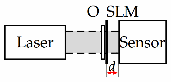
Figure 1: Optical setup corresponding to the considered data formation model: ’Laser’ is a broadband coherent light source, ’O’ is an object, ’SLM’ is a spatial light modulator ($\mathcal{M}_{t}$), and ’Sensor’ is a registration camera.

The free space propagation linking $U_{o,k}$ and $U_{t,k}$ is modeled by the angular spectrum operator calculated using the forward $\mathcal{F}\{\cdot\}$ and inverse $\mathcal{F}^{-1}\{\cdot\}$ Fourier transforms:

$$U_{t,k}=\mathcal{F}^{-1}\{AS\circ\mathcal{F}\{\mathcal{M}_{t}\circ U_{o,k}\}\},$$ (29)

where the angular spectrum transfer function in the $2D$ Fourier domain $(f_{x},f_{y})$ is defined according to [48] as:

$$AS=\left\{\begin{array}[l]{l}\exp(jkd\sqrt{1-(\lambda f_{x})^{2}-(\lambda f_{y})^{2}})\text{, }(\lambda f_{x})^{2}+(\lambda f_{y})^{2}\leq 1\\ 0\,\text{, otherwise}\end{array}\right.$$ (30)

Here, $d$ is a distance from the object to the sensor plane equal to $2$ mm (see Fig.1). In the discrete modeling, the sampling corresponds to the camera pixel size equal to $3.45~{}\mu$m.

The equations (29) and (30) are written for $2D$ variables, thus the coding phase mask $\mathcal{M}_{t}$ and the object $U_{o,k}$ are $2D$ complex-valued functions.

The HS wavefronts and measurements are modeled by propagating the broadband laser beam through the object and the phase modulation mask. Both of them are modeled by the complex-valued transfer function [48]:

$$g=a\circ\exp(-jkh(n_{\lambda}-1)),$$ (31)

where $k=2\pi/\lambda$, $h$ is a thickness of the object/mask, $n_{\lambda}$ is a refractive index depending on $\lambda$.

The phase delay of the wavefront propagating through $g$ is defined by the argument of the exponential function in (31). It is assumed in our tests that the amplitude $a$ and the thickness $h$ are spatially varying on $(x,y)$ but invariant with respect to the spectral (wavelength) arguments $k$ and $\lambda$. Nevertheless, the model (31) shows that the properties of the object and the masks are spectrally varying.

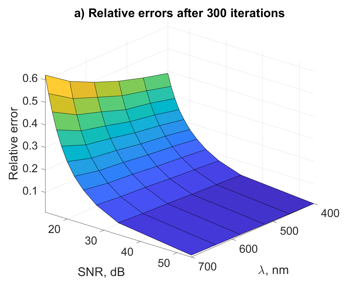
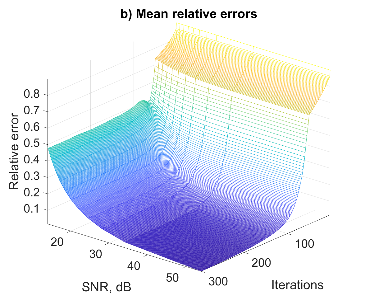
Figure 2: Relative error maps for the HSPhR algorithm, Gaussian noise: a) $ERROR_{rel}$ as function of SNR and wavelength; b) $ERROR_{rel}$ as function of SNR and iteration number. In b) $ERROR_{rel}$ is averaged over the wavelengths. The iterations on CCF and the Lagrange variables are disabled up to 50th iteration.

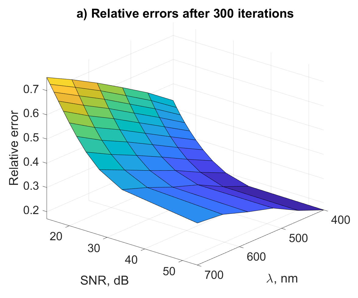
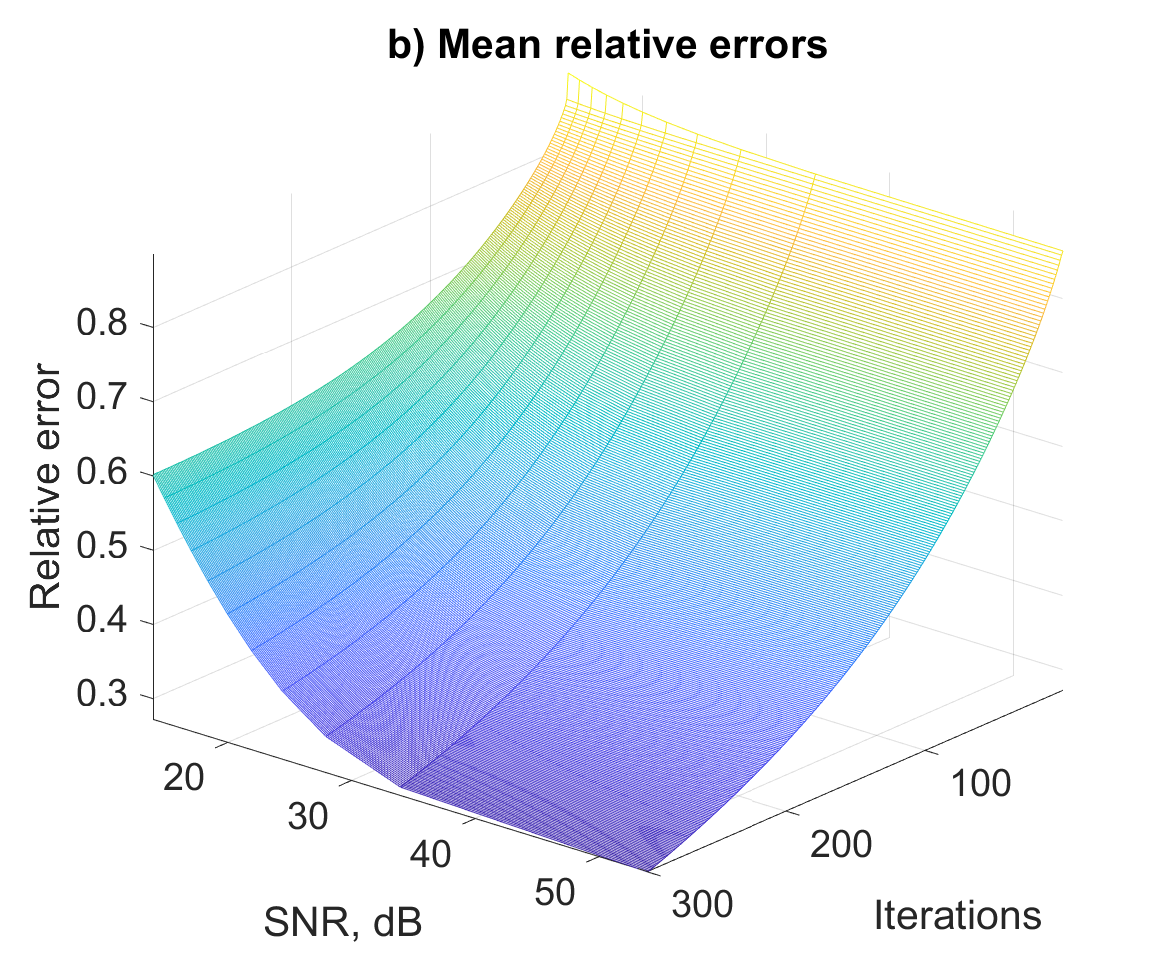
Figure 3: Relative error maps for the HSPhR algorithm with disabled iterations on the Lagrange variables and the CCF filter, Gaussian noise: a) $ERROR_{rel}$ as function of SNR and wavelength; b) $ERROR_{rel}$ as function of SNR and iteration number. In b) $ERROR_{rel}$ is averaged over the wavelengths. The achieved accuracy is much worse than that for the HSPhR algorithm with enabled iterations on the Lagrange variables and the CCF filter shown in Fig.2.

We assume that the amplitude and phase of the object are $64\times 64$ images: ’peppers’ for amplitude  and ’cameraman’ for phase. We take these images quite different to test how far phase and amplitude can be separated by the proposed algorithm. The phase is scaled in such way that the object phase delay for all $\lambda\in\Lambda$ would be in the range $[0$, $\pi]$. The amplitude $a$ is scaled to the interval $(0,1]$. For the coding mask, $a=1$, and $h$ is piece-wise invariant random with equal probabilities taking one of the following five values $[0,1,-1,1/2,-1/2]\cdot\lambda_{\min}/4$, where $\lambda_{\min}=400$ nm.

For each of the $T$ experiments, the masks are generated independently. Thus, overall we have $T$ different masks. The forward propagation (image formation) operator $A_{t,k}$ in (2) is defined by the propagation model (29) and the modulation masks. It is clear from the model (29) that the propagation model is wavelength varying. The same is true for the modulation mask, as it is fixed for each experiment, but its spectral properties vary with $\lambda$ according to (31). As the phase mask is included in the operator $A_{t,k}$, the complex-valued image at the sensor plane is defined as $U_{t,k}=A_{t,k}U_{o,k}$, where the object is also spectrally varying according to (31). The measured intensities are $Y_{t}=\sum_{k\in K}|U_{t,k}|^{2}$.

In our simulation, we assume that the refractive index in (31) as a function of $\lambda$ is known and calculated according to Cauchy’s equation [49] with parameters taken for the glass BK7 [50]. The input laser beam is uniform in both phase and amplitude, the amplitude is equal to $1$ and the phase is equal to $0$. We formulate the phase retrieval as the reconstruction of $U_{o,k}$.

The transfer function (31) is used for the calculation of the observations $Y_{t}$ and the phase delay in the masks, and is not used in the algorithm iterations.

We evaluate the accuracy of the complex-valued reconstruction by the relative error criterion introduced in [20]:

$$ERROR_{rel}=\min_{\varphi\in[0,2\pi)}||\hat{x}\circ\exp(j\varphi)-x||_{2}^{2}/||x||_{2}^{2},$$ (32)

where $x$ and $\hat{x}$ are the true signal and its estimate.

The efficiency of the developed algorithm is demonstrated in simulation tests with Gaussian and Poissonian observations. In these experiments we present the results achieved by the developed algorithms using both the Lagrange multipliers (Step 4) and the $CCF$ filtering (Step 6) as it is in the HSPhR algorithm , Subsection 2.4. In order to evaluate the value of these two key components of the algorithm, we show also results obtained when these components are disabled.

3.1 Accuracy as a function of $K$ and $N$.

A dependence of the algorithm accuracy on the wavelength number $K$ and the number of observations $T$ is of a special interest. In what follows, the noise level in observations is characterized by signal-to-noise ratio (SNR) in dB. We calculate the accuracy criterion $ERROR_{rel}$ for $K=[2,4,8,12]$ and $T=[2,6,12,24,36]$. The wavelengths for the varying $K$ (spectral channels) are defined as uniformly covering the interval $[400,700]$ nm. The number of iterations is fixed to $n=300$. The relative errors $ERROR_{rel}$ obtained in these experiments are shown in Table 1.

Table 1: $ERROR_{rel}$ versus number of experiments (masks) $T$ and wavelengths $K$; $\lambda=400$ nm; number of iterations $n=300$; $SNR=54$ dB

K\T	2	6	12	24	36
2	0.43	0.018	0.0062	0.0055	0.0061
4	0.68	0.097	0.011	0.0063	0.0074
8	0.82	0.34	0.084	0.013	0.0103
12	0.85	0.49	0.19	0.036	0.017

A larger value of $T$ for a fixed $K$ leads to more accurate reconstruction with smaller $ERROR_{rel}$. We found that visually a good phase imaging is achieved provided $ERROR_{rel}<0.1$. This threshold for $K=2$ is overcome for $T=6$. For $K=4,8,12$ it happens for $T=6,12,24$, respectively. Thus, we may conclude that $T\geq 3K$ is sufficient for the accuracy sufficient for good phase imaging. The results in Table 1 are given for nearly noiseless data with $SNR=54$ dB, but the conclusion that the inequality $T\geq 3K$ is sufficient for visually good phase imaging holds for noisy data also. This conclusion is one of the reasons to exploit in the forthcoming tests $T=18$ for $K=6$.

3.2 Gaussian observations

The relative error maps for the HSPhR algorithm are shown in Fig.2 for SNR taking values $[14:55]$ dB. The left image Fig. 2(a) demonstrates the accuracy as a function of $SNR$ and $\lambda$, while the right image Fig. 2(b) provides the accuracy as a function of $SNR$ and a number of iterations. In this latter image, the relative errors are averaged over $\lambda,K=6$. We may conclude from the left image that the acceptable quality imaging, $ERROR_{rel}<~{}0.1$, is achieved for all wavelengths provided that $SNR$ larger than 28 dB. The accuracy for smaller wavelengths is higher than the accuracy for larger values of wavelengths.

The convergence rate can be evaluated from the right image. After 200 iterations and for $SNR>28$ the accuracy becomes acceptable, $ERROR_{rel}<~{}0.1$. The bend in the accuracy map in Fig. 2(b) well seen at iteration 50 is of special interest. The algorithm’s iterations on CCF and the Lagrange variables are disabled in this experiment up to this 50th iteration. Thus, we can observe the dramatic improvement in the convergence rate due to CCF and the Lagrange variables. We introduce this delay in the activation of CCF and the Lagrange variables only for demonstration of their efficiency. They can be activated from the first iterations that improves the accuracy.

In Fig.3 we show the relative error maps provided that both the Lagrange variables and $CCF$ are disabled in the HS-CD-PhD algorithm completely. The degradation of the algorithm in values of $ERRORS_{rel}$ is clear in this case. In particular, it is demonstrated comparing the error maps in Fig.2 and Fig.3. The relative errors in Fig.3 are always larger than 0.1, i.e., the accuracy of imaging is not acceptable.

3.3 Poissonian observations

For the scenario identical to considered for the case of Gaussian noise, we introduce results obtained for Poissonian observations. The level of the noise is controlled by the parameter $\chi$ which takes values corresponding SNR in the interval $[14:44]$ dB. The maps of the relative errors are shown in Fig 4. The left image Fig. 4(a) demonstrates the accuracy as a function of $SNR$ and $\lambda$, while the right image Fig. 4(b) provides the accuracy as a function of $SNR$ and a number of iterations. In this latter image, the relative errors are averaged over $\lambda,K=6$. We may conclude from the left image that the acceptable quality imaging, $ERROR_{rel}<~{}0.1$, is achieved for all wavelengths provided that $SNR$ is larger than 32 dB. The convergence rate is well seen from the right image. After 150 iterations and for $SNR>32$ dB the accuracy becomes acceptable. A visual bend in the accuracy map in Fig. 4(b) happened at the 50th iteration demonstrates the effects of CCF and the Lagrange variables which are disabled up to the 50th iteration. We can observe the dramatic improvement in the convergence rate due to CCF and the Lagrange variables.

In Fig. 5 we demonstrate the results obtained by the algorithm where the Lagrange iterations and CCF filtering are disabled completely. Similar as it was discussed for the Gaussian case, we may note a serious degradation in the algorithm performance with $ERROR_{rel}>~{}0.2$, what confirms the essential role of both the Lagrange iterations and the CCF filtering for the algorithm performance.

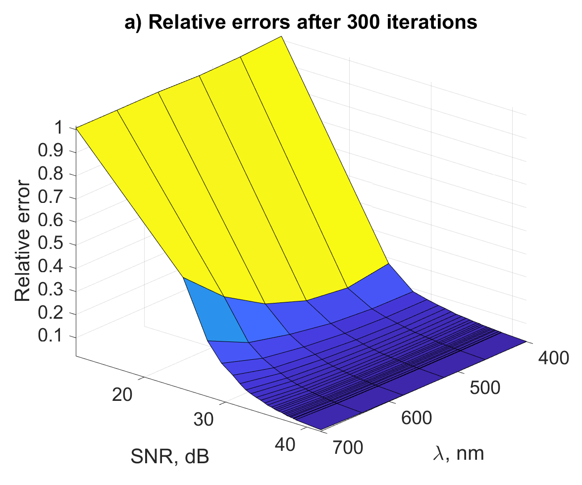
a)

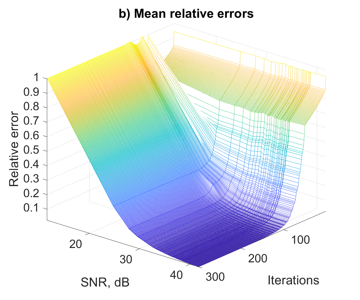
b)

Figure 4: HSPhR reconstruction relative error maps for the object wavefronts in the case of Poisson noise depending on: a) SNR and wavelength after 300 iterations; b) SNR and iteration number. In b) error values are represented as mean value for all wavelengths. The iterations on CCF and the Lagrange variables are disabled up to 50th iteration.

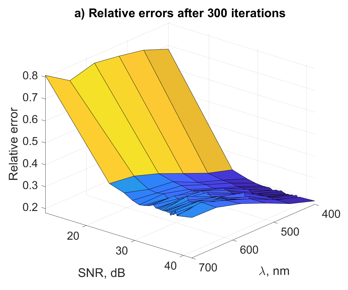
a)

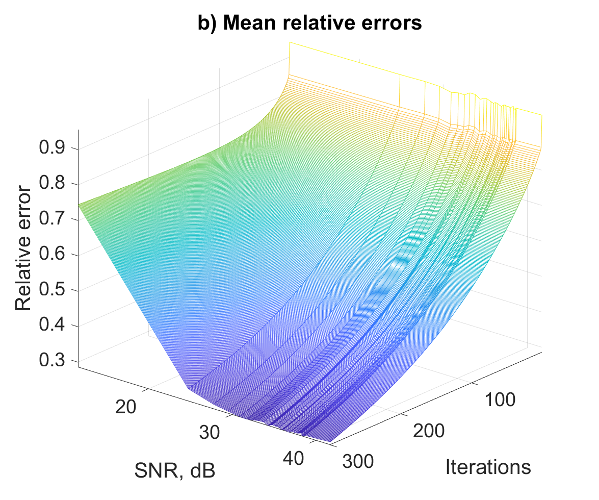
b)

Figure 5: The HSPhR algorithm with disabled the Lagrange iterations and CCF filtering. The reconstruction relative error maps for the object wavefronts in the case of Poisson noise depending on: a) SNR and wavelength after 300 iterations; b) SNR and iteration number. In b) error values are represented as mean value for all wavelengths.

3.4 Imaging

In this subsection, we evaluate the visual quality of reconstructions. The algorithm provides the HS broadband imaging, i.e. reconstruction of 3D complex-valued cubes. In Fig.6, we show 2D images of amplitude and phase for the middle wavelength of the interval $\Lambda$, $\lambda=640$ nm. It is a nearly noiseless case as SNR=54 dB. Fig. 6(a) provides the results for the Gaussian version of the algorithm and the Gaussian noisy data, and Fig. 6(b) provides the results for the Poissonian version of the algorithm and the Poissonian data. In all cases the images of the amplitude and phase of the high visual quality. The relative errors are low, equal to 0.019 and 0.018 for Gaussian and Poissonian data, respectively.

The images are shown in square frames in order to emphasize that the size and location of the object support are assumed being unknown and reconstructed automatically by the HSPhR algorithm. The true image’s support is used only for computation of observations produced for the zero-padded object and is not exploited in the algorithm’s iterations. For the amplitude images, these frames have nearly zero values, while the phase estimates take random values in the frame area as the phase cannot be defined for the amplitude is equal to zero. Practically, these variations of the phase do not influence the calculation of $ERROR_{rel}$ as the amplitude estimated quite accurately in these areas and close to zero. Nevertheless, $ERROR_{rel}$ shown in the images are calculated for the central parts of the images corresponding to the true location of the image support.

Fig.7 shows the results for the noisy cases of SNR=34 dB. With this level of SNR, the noise effects are appeared to be essential. The relative errors are much higher with 0.058 and 0.08 for Gaussian and Poissonian data, respectively.

In Fig.8 we show the images obtained by the HSPhR algorithm for the same noisy scenario, SNR=34 dB, with the Lagrange iterations and CCF filtering disabled. The obtained amplitude/phase images are very noisy, the visual quality of imaging is low, as compared with the results in Fig.7. The relative errors take higher values equal to 0.39 and 0.36 for Gaussian and Poissonian observations, respectively. These experiments provide a visual and numerical confirmation of the discussed above role of the Lagrange iterations and CCF filtering as the key components of the HSPhR algorithm.

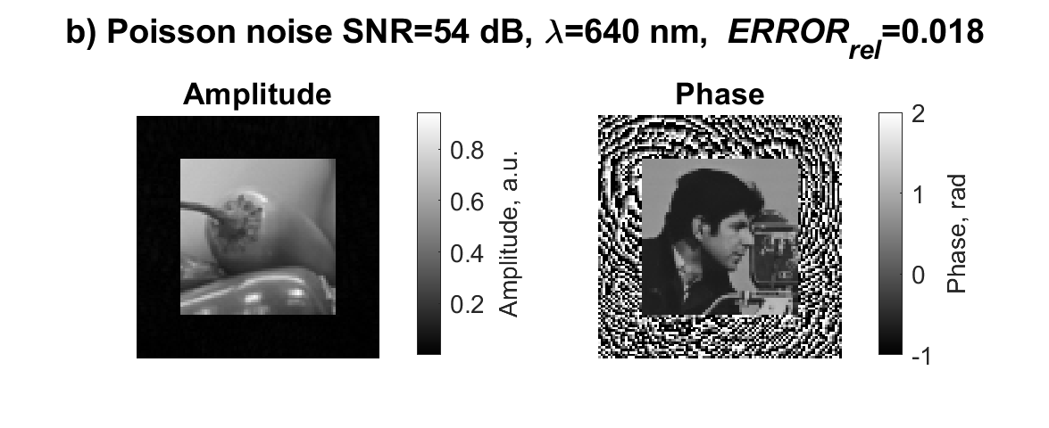
Figure 6: HSPhR amplitude and phase reconstructions, nearly noiseless case (SNR=54 dB): a) Gaussian and b) Poisson versions of the algorithm; $\lambda=640$ nm; iteration number $n=300$.

Figure 7: HSPhR amplitude and phase reconstructions, noisy observations (SNR=34 dB): a) Gaussian and b) Poisson versions of the algorithm; $\lambda=640$ nm; iteration number $n=300$.

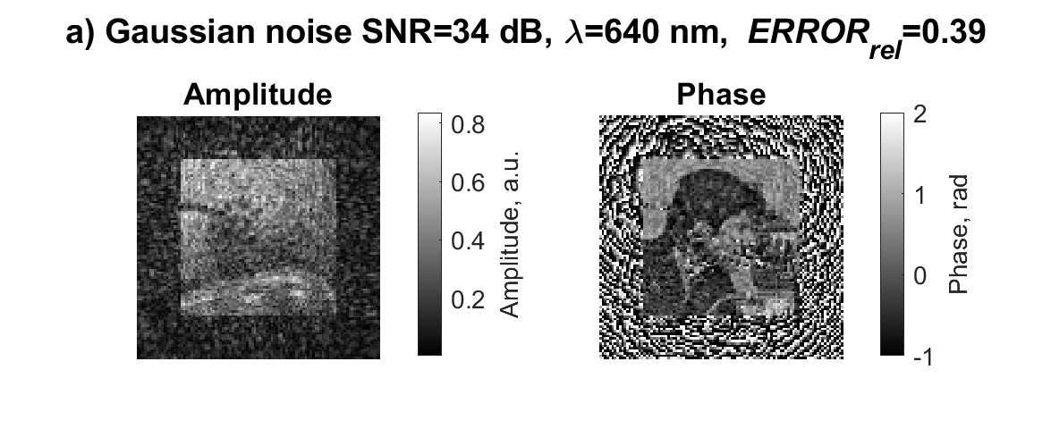
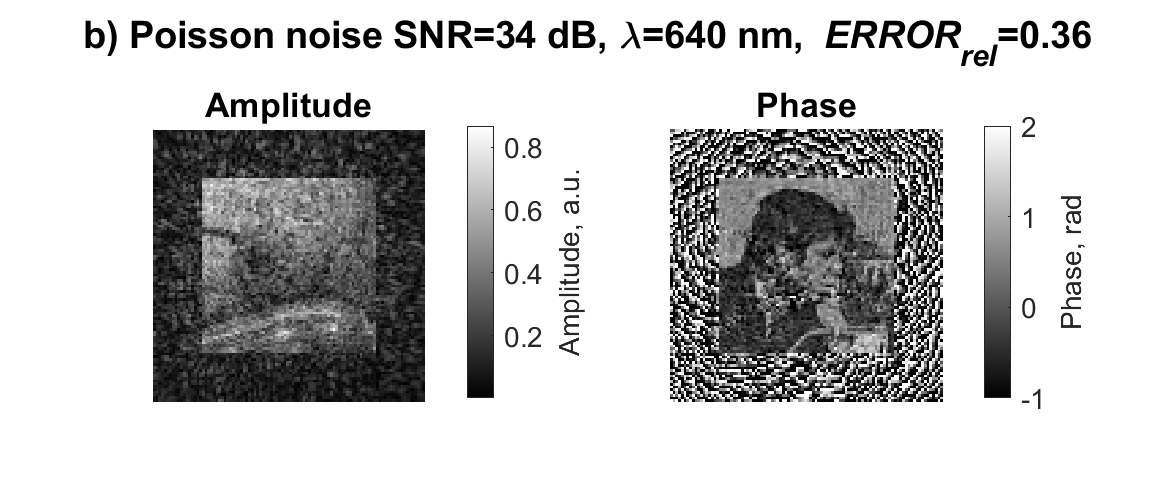
Figure 8: HSPhR amplitude and phase reconstructions, with disabled iterations on the Lagrange variables and the CCF filter; noisy observations (SNR=34 dB): a) Gaussian and b) Poisson versions of the algorithm; $\lambda=640$ nm; iteration number $n=300$. The obtained images are very noisy, in particular, as compared with the results in Fig.7.

The complexity of the algorithm is characterized by the computational time per iteration required for the test images, $K=6$, $T=18$. This time is equal to 0.8 sec. for calculations without CCF and equal to 21.5 sec. for calculations with CCF. All calculations are done in MATLAB R2019b on a computer with 32 GB of RAM and CPU with a 3.40 GHz IntelR CoreTM i7-3770 processor. We will make publicly available the MATLAB demo-code of the developed algorithm.

4 Conclusion

A novel formulation of the HS broadband phase retrieval problem is proposed, where both object and image formation operators are spatially and spectrally varying. The proposed algorithm is based on the complex domain version of the ADMM technique. The derived Spectral Proximity Operators and the CCF noise suppression are important elements of this algorithm. The SPOs are defined for Gaussian and Poissonian observations and calculated solving the sets of cubic (for Gaussian) and quadratic (for Poissonian) algebraic equations. The ability to resolve the HS phase retrieval problem and to find the spectral varying object components $U_{o,k}$, $k\in K$, completely depends on spectral properties of the spectral channels $A_{t,k}$ and of the object $U_{o,k}$. The model of the object is not used in the algorithm and the modulation phase masks are calculated in advance and fixed in the algorithm iterations. The simulation tests demonstrate that the HS phase retrieval in this formulation can be resolved with quite general modeling of object and image formation operators. The MATLAB demo-codes of the developed algorithm are made publicly available.

Funding

This work is a part of the CIWIL project funded by the Technology Industries of Finland Centennial Foundation and Jane and Aatos Erkko Foundation.

References

- [1] M. J. Khan, H. S. Khan, A. Yousaf, K. Khurshid, and A. Abbas, “Modern Trends in Hyperspectral Image Analysis: A Review,” IEEE Access, vol. 6, pp. 14 118–14 129, 2018.
- [2] M. Paoletti, J. Haut, J. Plaza, and A. Plaza, “Deep learning classifiers for hyperspectral imaging: A review,” ISPRS Journal of Photogrammetry and Remote Sensing, vol. 158, pp. 279–317, 12 2019.
- [3] B. Fei, “Hyperspectral imaging in medical applications,” in Data Handling in Science and Technology. Elsevier Ltd, 1 2020, vol. 32, pp. 523–565.
- [4] S. G. Kalenkov, G. S. Kalenkov, and A. E. Shtanko, “Holographic fourier transform spectroscopy of biosamples,” Optics InfoBase Conference Papers, p. 3, 2014.
- [5] ——, “Hyperspectral holography: an alternative application of the Fourier transform spectrometer,” Journal of the Optical Society of America B, vol. 34, no. 5, pp. B49–B55, 2017. [Online]. Available: https://www.osapublishing.org/abstract.cfm?URI=josab-34-5-B49
- [6] M. Mir, B. Bhaduri, R. Wang, R. Zhu, and G. Popescu, “Quantitative Phase Imaging,” in Progress in Optics, 2012, vol. 57, pp. 133–217.
- [7] T. Cacace, V. Bianco, and P. Ferraro, “Quantitative phase imaging trends in biomedical applications,” Optics and Lasers in Engineering, vol. 135, p. 106188, 12 2020.
- [8] M. R. Kellman, E. Bostan, N. A. Repina, and L. Waller, “Physics-Based Learned Design: Optimized Coded-Illumination for Quantitative Phase Imaging,” IEEE Transactions on Computational Imaging, vol. 5, no. 3, pp. 344–353, 9 2019.
- [9] M. Trusiak, M. Cywińska, V. Micó, J. A. Picazo-Bueno, C. Zuo, P. Zdańkowski, and K. Patorski, “Variational Hilbert Quantitative Phase Imaging,” Scientific Reports, vol. 10, no. 1, p. 13955, 12 2020.
- [10] D. Claus, G. Pedrini, D. Buchta, and W. Osten, “Accuracy enhanced and synthetic wavelength adjustable optical metrology via spectrally resolved digital holography,” Journal of the Optical Society of America A: Optics and Image Science, and Vision, vol. 35, no. 4, pp. 546–552, 2018.
- [11] B. Kemper, D. Carl, J. Schnekenburger, I. Bredebusch, M. Schäfer, W. Domschke, and G. von Bally, “Investigation of living pancreas tumor cells by digital holographic microscopy.” Journal of biomedical optics, vol. 11, no. 3, p. 34005, 1 2006. [Online]. Available: http://biomedicaloptics.spiedigitallibrary.org/article.aspx?articleid=1102204
- [12] T. Tahara, X. Quan, R. Otani, Y. Takaki, and O. Matoba, “Digital holography and its multidimensional imaging applications: A review,” pp. 55–67, 4 2018.
- [13] Y. Baek and Y. Park, “Scaling down quantitative phase imaging,” Nature Photonics, vol. 14, no. 2, pp. 67–68, 2020.
- [14] Y. Park, C. Depeursinge, and G. Popescu, “Quantitative phase imaging in biomedicine,” Nature Photonics, vol. 12, no. 10, pp. 578–589, 10 2018.
- [15] B. Kemper, A. Barroso, S. Ketelhut, L. Kastl, J. Schnekenburger, and P. Heiduschka, “Hyperspectral digital holographic microscopy approach for reduction of coherence induced disturbances in quantitative phase imaging of biological specimens,” in Speckle 2018: VII International Conference on Speckle Metrology, M. Józwik, L. R. Jaroszewicz, and M. Kujawińska, Eds. SPIE, 9 2018, p. 49.
- [16] C. Ba, J.-M. Tsang, and J. Mertz, “Fast hyperspectral phase and amplitude imaging in scattering tissue,” Optics Letters, vol. 43, no. 9, p. 2058, 2018.
- [17] K. B. Yushkov, J. Champagne, J.-C. Kastelik, O. Y. Makarov, and V. Y. Molchanov, “AOTF-based hyperspectral imaging phase microscopy,” Biomedical Optics Express, vol. 11, no. 12, p. 7053, 12 2020.
- [18] R. W. Gerchberg and W. O. Saxton, “A Practical Algorithm for the Determination of Phase from Image and Diffraction Plane Pictures,” Phys. E. ppl. Opt. OPTIK, vol. 2, no. 352, pp. 237–246, 1969. [Online]. Available: http://www.u.arizona.edu/ ppoon/GerchbergandSaxton1972.pdf
- [19] J. R. Fienup, “Phase retrieval algorithms: a comparison,” Applied optics, vol. 21, no. 15, pp. 2758–2769, 8 1982. [Online]. Available: https://www.osapublishing.org/abstract.cfm?URI=ao-21-15-2758 http://www.ncbi.nlm.nih.gov/pubmed/20396114
- [20] E. Candes and M. Wakin, “An Introduction To Compressive Sampling,” IEEE Signal Processing Magazine, vol. 25, no. 2, pp. 21–30, 2008.
- [21] Y. Shechtman, Y. C. Eldar, O. Cohen, H. N. Chapman, J. Miao, and M. Segev, “Phase Retrieval with Application to Optical Imaging: A contemporary overview,” IEEE Signal Processing Magazine, vol. 32, no. 3, pp. 87–109, 5 2015.
- [22] G. Wang, G. B. Giannakis, and J. Chen, “Solving large-scale systems of random quadratic equations via stochastic truncated amplitude flow,” in 2017 25th European Signal Processing Conference (EUSIPCO), vol. 2017-Janua, no. 2. IEEE, 8 2017, pp. 1420–1424.
- [23] A. Guerrero, S. Pinilla, and H. Arguello, “Phase Recovery Guarantees from Designed Coded Diffraction Patterns in Optical Imaging,” IEEE Transactions on Image Processing, vol. 29, pp. 5687–5697, 2020.
- [24] Z. Cai, R. Hyder, and M. S. Asif, “Learning Illumination Patterns for Coded Diffraction Phase Retrieval,” arXiv, 6 2020.
- [25] P. Grohs, S. Koppensteiner, and M. Rathmair, “Phase Retrieval: Uniqueness and Stability,” SIAM Review, vol. 62, no. 2, pp. 301–350, 1 2020.
- [26] A. Fannjiang and T. Strohmer, “The Numerics of Phase Retrieval,” Acta Numerica, vol. 29, pp. 125–228, 4 2020.
- [27] N. Vaswani, “Nonconvex Structured Phase Retrieval: A Focus on Provably Correct Approaches,” IEEE Signal Processing Magazine, vol. 37, no. 5, pp. 67–77, 9 2020.
- [28] B. Roig-Solvas, L. Makowski, and D. H. Brooks, “A proximal operator for multispectral phase retrieval problems,” SIAM Journal on Optimization, vol. 29, no. 4, pp. 2594–2607, 2019.
- [29] C. Dorrer, N. Belabas, J.-P. Likforman, and M. Joffre, “Spectral resolution and sampling issues in Fourier-transform spectral interferometry,” Journal of the Optical Society of America B, vol. 17, no. 10, p. 1795, 10 2000.
- [30] S. G. Kalenkov, G. S. Kalenkov, and A. E. Shtanko, “Spectrally-spatial fourier-holography,” Optics Express, vol. 21, no. 21, p. 24985, 10 2013.
- [31] I. Shevkunov, V. Katkovnik, D. Claus, G. Pedrini, N. V. Petrov, and K. Egiazarian, “Hyperspectral phase imaging based on denoising in complex-valued eigensubspace,” Optics and Lasers in Engineering, vol. 127, no. September 2019, pp. 105 973–105 982, 4 2020.
- [32] S. G. Kalenkov, G. S. Kalenkov, and A. E. Shtanko, “Self-reference hyperspectral holographic microscopy,” Journal of the Optical Society of America A, vol. 36, no. 2, p. A34, 2 2019.
- [33] I. Shevkunov, V. Katkovnik, and K. Egiazarian, “Lensless hyperspectral phase imaging in a self-reference setup based on Fourier transform spectroscopy and noise suppression,” Optics Express, vol. 28, no. 12, p. 17944, 2020.
- [34] V. Katkovnik, I. Shevkunov, and K. Egiazarian, “Broadband Hyperspectral Phase Retrieval From Noisy Data,” in 2020 IEEE International Conference on Image Processing (ICIP), no. 1. IEEE, 10 2020, pp. 3154–3158.
- [35] M. R. Hestenes, “Multiplier and gradient methods,” Journal of Optimization Theory and Applications, vol. 4, no. 5, pp. 303–320, 11 1969.
- [36] J. Eckstein and D. P. Bertsekas, “On the Douglas—Rachford splitting method and the proximal point algorithm for maximal monotone operators,” Mathematical Programming, vol. 55, no. 1-3, pp. 293–318, 4 1992.
- [37] M. V. Afonso, J. M. Bioucas-Dias, and M. A. T. Figueiredo, “Fast Image Recovery Using Variable Splitting and Constrained Optimization,” IEEE Transactions on Image Processing, vol. 19, no. 9, pp. 2345–2356, 9 2010.
- [38] ——, “An Augmented Lagrangian Approach to the Constrained Optimization Formulation of Imaging Inverse Problems,” IEEE Transactions on Image Processing, vol. 20, no. 3, pp. 681–695, 3 2011.
- [39] L. Li, X. Wang, and G. Wang, “Alternating Direction Method of Multipliers for Separable Convex Optimization of Real Functions in Complex Variables,” Mathematical Problems in Engineering, vol. 2015, pp. 1–14, 2015.
- [40] N. Parikh and S. Boyd, “Proximal Algorithms,” Foundations and Trends® in Optimization, vol. 1, no. 3, pp. 127–239, 2014.
- [41] F. Soulez, E. Thiebaut, A. Schutz, A. Ferrari, F. Courbin, and M. Unser, “Proximity operators for phase retrieval,” Applied Optics, vol. 55, no. 26, p. 7412, 9 2016.
- [42] V. Katkovnik, “Phase retrieval from noisy data based on sparse approximation of object phase and amplitude,” arXiv:1709.01071, 9 2017. [Online]. Available: http://arxiv.org/abs/1709.01071
- [43] C. A. Metzler, A. Maleki, and R. G. Baraniuk, “BM3D-PRGAMP: Compressive phase retrieval based on BM3D denoising,” in Proceedings - International Conference on Image Processing, ICIP, vol. 2016-Augus. IEEE Computer Society, 8 2016, pp. 2504–2508.
- [44] I. Shevkunov, V. Katkovnik, D. Claus, G. Pedrini, N. V. Petrov, and K. Egiazarian, “Spectral Object Recognition in Hyperspectral Holography with Complex-Domain Denoising,” Sensors, vol. 19, no. 23, p. 5188, 11 2019.
- [45] V. Katkovnik and K. Egiazarian, “Sparse phase imaging based on complex domain nonlocal BM3D techniques,” Digital Signal Processing: A Review Journal, vol. 63, pp. 72–85, 4 2017. [Online]. Available: https://www.sciencedirect.com/science/article/pii/S1051200417300052
- [46] V. Katkovnik, M. Ponomarenko, and K. Egiazarian, “Complex-valued image denosing based on group-wise complex-domain sparsity,” arXiv preprint arXiv:1711.00362, 2017.
- [47] K. Dabov, A. Foi, V. Katkovnik, and K. Egiazarian, “Image Denoising by Sparse 3-D Transform-Domain Collaborative Filtering,” IEEE Transactions on Image Processing, vol. 16, no. 8, pp. 2080–2095, 8 2007.
- [48] J. Goodman, Introduction to Fourier optics. Roberts & Co, 2005.
- [49] M. Born and E. Wolf, Principles of optics: electromagnetic theory of propagation, interference and diffraction of light. Elsevier, 2013.
- [50] P. Hartmann, Optical glass. SPIE PRESS BOOK, 2014.