Efficient and accurate group testing via Belief Propagation: an empirical study
Abstract.
The group testing problem asks for efficient pooling schemes and algorithms that allow to screen moderately large numbers of samples for rare infections. The goal is to accurately identify the infected samples while conducting the least possible number of tests. Exploring the use of techniques centred around the Belief Propagation message passing algorithm, we suggest a new test design that significantly increases the accuracy of the results. The new design comes with Belief Propagation as an efficient inference algorithm. Aiming for results on practical rather than asymptotic problem sizes, we conduct an experimental study. MSc: 05C80, 60B20, 68P30
1. Introduction
1.1. The group testing problem
In science generally and in applied science particularly there is much to be said for simplicity. But occasionally a modest degree of sophistication carries extraordinary rewards. Group testing is a case in point. Every single day medical labs around the globe screen moderately large numbers of samples for rare pathogens. The vast majority of samples, anywhere between 90% and 99.9%, are actually uninfected [7, 25, 28, 32, 35, 36, 37, 38, 39]. Labs therefore test pools of samples rather than individual samples. The group testing problem asks for pooling strategies that minimise the total number of tests required while maximising the accuracy of the results. The latter is crucial because test results are generally not perfectly accurate.
Coming up with practical solutions to this problem turns out to be challenging precisely because the total number of samples in a real-world scenario is moderate–say, in the hundreds or thousands. To elaborate, on the one hand the group testing problem has inspired a body of beautiful mathematical work that deals with the asymptotical scenario where the number of samples grows to infinity [4, 10, 11]. However, such asymptotical results do not directly bear on practical problem sizes. Besides, the theoretical test designs tend to suffer other drawbacks such as asking for excessively large test pools or subdivisions of individual samples into very many sub-samples [4, 10, 11]. On the other hand, practical problem sizes far exceed the limits up to which an exhaustive search for an optimal test design seems remotely feasible. As a consequence, the pooling schemes in practical use remain the self-same extremely simple ones suggested in the 1940s [7, 25, 28, 32, 35, 36, 37, 38, 39].
The aim of this paper is to investigate better test designs for practical problem sizes. The focus is on improving the accuracy of the results, i.e., avoiding false positive and/or negative diagnoses while keeping the number of tests as small as possible. Indeed, the thrust of this paper is that the idea of group testing, originally invented to reduce the number of tests, actually excels at improving the accuracy of the results. This may seem surprising at first glance because one might deem individual testing optimal in terms of accuracy. It is not. Group testing does better in much the same way as error-correcting codes gain power from encoding entire blocks of data simultaneously.
Given the moderate number of samples in real-world scenarios, an empirical approach is the only feasible way to obtain practically meaningful results. Thus, taking on board the intuition from theoretical work on group testing as well as recent ideas from information theory and statistical physics, we conduct an extensive experimental study. The main finding is that a novel test scheme called adaptive Belief Propagation greatly improves the accuracy of the overall results while keeping the number of tests conducted low. Furthermore, the new test design requires only relatively small test pools and only assigns each sample to a small number of tests. Finally, the design comes with an efficient, easy-to-implement algorithm to infer the status of the individual samples from the test results, namely the Belief Propagation message passing algorithm.
We proceed to discuss the mathematical model of tests and samples that we work with. Subsequently, we present the results of adaptive Belief Propagation by comparison to other test schemes. These test schemes, which are partly incorporated into adaptive Belief Propagation, are discussed in detail in Section 2. In Section 3 we then present the new test design and the corresponding inference algorithm. Section 4 details the theoretical and heuristical considerations that underpin adaptive Belief Propagation. Finally, in Section 5 we discuss the potential impact of the new results and future directions for both empirical and theoretical work.
1.2. The model
We work with a simple but standard model of group testing that allows for test results to not be entirely accurate [4]. Let represent the samples submitted for testing. We assume that with a prior probability of any one sample is infected is known. The true infection status of each sample is indicated by , with representing ‘infected’. The are assumed to be independent Bernoulli variables with mean . We refer to the vector as the ground truth. Let signify the actual number of infected samples.
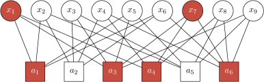
The way how test pools are formed is represented by a bipartite graph. To be precise, a test design is a bipartite graph with one class of vertices representing the samples and the other class representing the test pools. An edge between and indicates that is included in test pool . For each we let be the set of test pools that include . Similarly, for each test pool we write for the set of individual samples included in that pool.
Each test reports a positive or negative result . Ideally a test should come back positive iff at least one sample is actually infected. But the test results need not be completely accurate. We therefore posit two parameters , called the specificity, and , the sensitivity, both between and , such that the tests return results
| (1.1) | |||||
| (1.2) |
The random outcomes in (1.1)–(1.2) are mutually independent given . Let encompass the test results.
Generally the ground truth cannot be inferred with perfect accuracy form the test results of a single “one-shot” test design (unless and we test every separately) [1]. Indeed, under the noise model (1.1)–(1.2) the posterior of the ground truth given the test results reads111In (1.3) the -symbol hides the normalisation required to turn into a probability distribution.
| (1.3) | ||||
| where | (1.4) |
Hence, the information-theoretically optimal inference algorithm just draws a random sample from the distribution . In effect, the accuracy with which the ground truth can potentially be recovered is governed by the entropy of the posterior : the smaller the entropy the better the results. Furthermore, depending on the specific design there may or may not exists an efficient algorithm for sampling from .
To deal with these challenges, in adaptive group testing tests are not deployed in a single stage like in (1.1)–(1.2) but in several stages. To be precise, an -stage test design is an increasing sequence of test designs such that is obtained from by adding further tests. How many tests are added and which samples they contain depends on results from the previous stages. The results of the new tests are assumed to be distributed independently according to (1.1)–(1.2). The aim, of course, is to diligently add tests so as to maximally reduce the entropy of the posterior.
In summary, the group testing problem poses the following challenges.
-
(i)
To come up with an adaptive test design that allows to infer the true infection status of as many as possible while conducting as small a number of tests as possible.
-
(ii)
To devise an efficient algorithm that actually infers the from the observed with reasonable computational effort.
-
(iii)
To facilitate practical adoption we need to avoid high degrees because very large test pools may be infeasible, as may be dividing an individual sample into very many pools.
-
(iv)
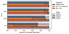
To ensure a timely reporting of test outcomes we should aim for a small number of test stages, or at least ensure that most samples can be diagnosed after the first or second stage.
1.3. Results
To meet these objectives we devise a new test scheme called adaptive Belief Propagation. We investigate its performance empirically for the following parameter choices.
-
•
The results in this section refer to samples. In Section 4.3 we discuss that the performance is similar on instances with and slightly better with .
-
•
We study prior infection probabilities .
- •
-
•
Each experiment is run times independently for each parameter combination.
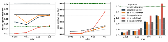
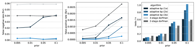
The experiments show that adaptive Belief Propagation improves the accuracy of the results by an order of magnitude by comparison to known test designs while keeping the number of tests at a reasonable level. Let us begin with the high-noise scenario , where we reap the greatest gains. We propose three different test designs adaptive Belief Propagation 1, adaptive Belief Propagation 2 and adaptive Belief Propagation 3. The first strikes a balance between accuracy of results and the number of tests, while the latter emphasises accuracy. In the following, let the false positive rate (fpr) be the number of healthy samples falsely classified as infected over all healthy samples. Correspondingly, let the false negative rate (fnr) be the number of infected samples falsely classified as healthy over all infected samples. Figure 1 displays the results of adaptive Belief Propagation 1 in comparison to several previously known approaches. These include the 2-stage Dorfman and the 3-stage Dorfman designs, which are widely used in practice, as well as Belief Propagation followed by individual testing advocated in the theoretical literature 222Note that with perfectly reliable tests, this approach is equivalent to the so-called definite defectives (DD) algorithm followed by individual testing.. A further scheme that we included is informative Dorfman, a 2-stage design proposed in [29]. We will discuss these approaches in some detail in Section 2. Figure 1 shows that with about the same number of tests as 2-stage Dorfman, adaptive Belief Propagation achieves up to reduction in the number of false positives and an up to reduction in the number of false negatives. The gains are particularly high for small priors.
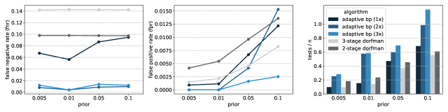
Nevertheless, the absolute value of the false positive and false negative rate of all test designs in Figure 1, particularly for large priors, may still be unacceptably high for many real-world applications. Here our other two designs adaptive Belief Propagation 2 and adaptive Belief Propagation 3 come to the rescue. As Figure 2 shows, these designs, particularly adaptive Belief Propagation 3, dramatically reduce the number of false positives and negatives. Of course, these improvements come at the expense of a larger number of tests. But for priors the number of extra tests is moderate, and for the largest prior adaptive Belief Propagation 2 and adaptive Belief Propagation 3 require not many more tests than individual testing while being the only designs that deliver decent accuracy.
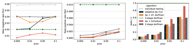
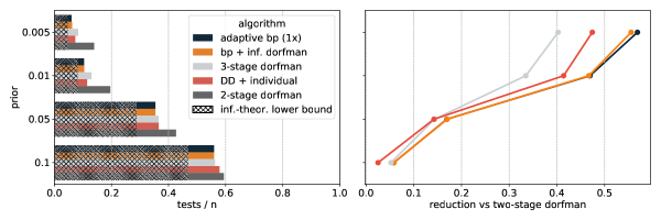
Matters turns out similar in the case of moderately high sensitivity and specificity , . Figure 3 displays the results. In comparison to the classical two- and three-stage Dorfman scheme, adaptive Belief Propagation requires at most more tests for high priors of - for small priors even fewer tests. The benefit is that adaptive Belief Propagation boosts accuracy compared to all the previously known designs, particularly so for low priors. We point out that the gains vis-a-vis informative Dorfman for moderately high priors are modest. The key benefit in adaptive Belief Propagation however, lies in its versatility to meaningfully enhance the accuracy at the expense of somewhat more tests as shown in Figure 4. A similar extension of informative Dorfman would yield a similar accuracy but require significantly more tests than adaptive Belief Propagation.
Even with perfectly reliable tests, the conventional definite defectives (DD) approach in the literature can be improved upon by adaptive Belief Propagation or the informative Dorfman approach. Both schemes are able to reduce the number of tests compared to the former by up to and comes within to of the information-theoretic lower bound. The gains vis-a-vis two-stage Dorfman with up to and individual testing with up to are even more pronounced. We do not need to consider the accuracy in the noiseless case since all test designs recover the entire ground truth by construction.
All examined algorithms require reasonable pool sizes and splits of the individual sample that are in line with common pooling procedures [22, 24, 29]. The maximum pool size is between and depending on noise level and prior, while the splits of the individual sample range between and . It should be noted that the proposed algorithms and test designs can readily be adjusted to accommodate smaller pool sizes or individual sample splits — at the expense of somewhat more tests.
Organisation
In Section 2, we will discuss designs and algorithms that are in practical use or have been studied in the mathematical literature on group testing. Subsequently, we present the details behind our novel test design named adaptive Belief Propagation in Section 3. In Section 4 we relate adaptive Belief Propagation to the theoretical work on group testing and asymptotic considerations.
2. Designs and algorithms
We discuss the various previously studied test designs and inference algorithms. In Section 3 we will then see how we extend and modify these known constructions in order to obtain the new adaptive Belief Propagation design.
2.1. Individual testing
The most straightforward test strategy, of course, is to conduct individual tests for each of the samples. At first glance, individual testing may appear to be the gold standard in terms of accuracy. Naturally, in the case , individual testing will register the status of each sample correctly. However, realistic values for and range between and [7, 8, 31, 38, 41]. If are less than one, then individual testing will produce numbers of false positives/negatives distributed as and , respectively.
The accuracy of the results could obviously be boosted by conducting two or three individual tests per sample. Indeed, if we test each twice and report as infected only if both tests come back positive, then we could reduce the expected number of false positives to . But we would now expect a slightly larger number of false negatives. To reduce the number of false positives and negatives simultaneously we could test each thrice and report the majority of the three test results.
2.2. Dorfman and grid designs
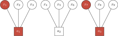
The test designs that currently appear to be most widely used in practice date back to the 1940s. Indeed, the idea of group testing was first brought up by Dorfman in 1943 [18]. He suggested a two-stage test procedure. In the first stage, every sample gets placed in precisely one pool. All pools are the same size, which depends on the prior only. Pools with a positive test result get tested separately in the second stage. An illustration is provided in Figure 6. Depending on the prior, this scheme can significantly reduce the number of tests required. For example, with this scheme uses pools of size five and the expected overall number of tests conducted in both stages comes to about . At the same time, Dorfman’s two-stage procedure reduces the number of false positives because a sample is ultimately reported as positive only if both the tests are positive. But for the same reason, the expected number of false negatives increases. For instance, with and as above, we expect false positives and false negatives.
A natural extension of the Dorfman procedure employs three stages. In the first stage, relatively large pools are formed. The second stage then splits the positive ones into smaller sub-pools and the third stage resorts to individual testing. In effect, as with the two-stage procedure, the expected number of false positives drops while the expected number of false negatives increases. For and as above the expected numbers of false positives/negatives work out to be and , respectively.
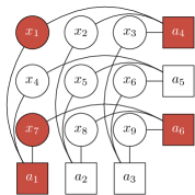
Grid designs are a variation on the Dorfman scheme. They partition the set of all individual samples into equal-sized subsets. For instance, if the size would be 16. Each of these subsets is mapped onto a grid. Its rows and columns constitute the pools for the first stage. Thus, each sample lands in two first-stage pools. Depending on the results, further tests are conducted in a second stage; see Figure 6 for an illustration. Grid designs significantly reduce the number of false negatives by comparison to individual testing while increasing the number of false positives. However, the number of tests required exceeds that of the two-stage Dorfman procedure.
2.3. Probabilistic constructions
More sophisticated test designs have been proposed in the mathematical theory of group testing. The best current, and in certain asymptotic settings provably optimal, test designs harness randomisation [4, 11]. For instance, in the random biregular test design every test pool has an equal size and every individual sample joins an equal number of pools; see Figure 7 for an illustration. In other words, the test design is chosen uniformly at random from the set of all -regular bipartite graphs [21].333To be precise, is typically drawn from the pairing model of graphs with given degrees. In this model, it is rare but possible that the same individual joins a test pool twice. In practice, such double occurrence could, of course, be reduced to single occurrences. In order to extract the maximum amount of information about the ground truth, the parameters should be chosen so as to maximise the conditional entropy of the vector of test results. Hence, should be chosen so that about half the tests will be positive:444Of course, due to rounding issues we cannot ensure that the expected number of positive tests is precisely equal to .
| (2.1) |
Why does such a randomised construction seem promising? Intuitively the randomness of the test design reduces dependencies between the different test results to a minimum. Thus, with chosen as above and for a number of tests up to a certain threshold, we can hope to squeeze as much as one bit’s worth of information from each test. Similar randomised constructions have proved powerful in coding theory and compressed sensing as well [16, 15, 26, 34].
While in the designs that we discussed previously obvious inference algorithms suggested themselves, in the case of the random biregular design matters are not quite so straightforward. In the case maximum a posteriori inference boils down to a minimum hypergraph vertex cover problem [10]. However, this problem is NP-hard and even on random instances no efficient algorithm is known.
A blunt but efficient algorithm that has been analysed in the case goes by the name of definite defectives (‘’) [3]. The algorithm classifies as infected every sample that is included in positive test pools only and that appears in at least one positive test pool where all other samples appear in a negative test. All other samples are classified as uninfected. In symbols,
For this algorithm will never produce false positives but may render false negatives. Several similarly-flavoured algorithms have been analysed mathematically. Aldridge analysed an adaptive test design whose different stages employ random biregular test designs with suitably chosen degrees [2]. This adaptive test design carried out over an unbounded number of stages achieves rates in excess of bits per tests. However, the large number of stages might render the scheme impractical.
2.4. Glauber dynamics
The algorithm merely extracts binary information about each sample. For a more fine-grained picture we would need to get a better handle on the posterior distribution (1.3) of the random test design. An immediate idea is to use a Markov Chain Monte Carlo algorithm to approximate the marginals of the posterior. Specifically, the Glauber dynamics starts at a random initial configuration drawn from the prior. Thus, the individual are independent variables. Glauber then proceeds to generate a random sequence of configurations by updating the status of a random sample at each time step according to (1.3); see [27] for a detailed derivation of the Glauber update rule. The hope is that for moderate the empirical means of the sequence approximate the actual posteriors well, i.e.,
| (2.2) |
At this point, no mathematical analysis of Glauber exists. Furthermore, an empirical assessment of (2.2) is difficult because even for moderate values of we cannot hope to compute the marginals of the posterior (1.3) exactly by exhaustive enumeration. Nonetheless, an experimental study of Glauber has been conducted in [14].
2.5. Informative Dorfman
Even if we assume that Glauber (or some other algorithm) approximates the posterior marginals well, how could we use this information in the second stage? A simple idea is to revisit the original Dorfman design. Hence, equipped with the posterior marginals from the first round, we could set up test pools such that each sample gets placed in precisely one pool. But now we could try to take the posteriors from the first stage into consideration in compiling the pools. Finally, just like in the original Dorfman scheme one could test the samples in each pool that returns a positive result separately. This procedure goes by the name of informative Dorfman [29].
How exactly do we take advantage of the marginals to set up the pools? A natural idea is to sort the samples increasingly according to their marginals and pool them in this order. A simple optimisation given the sequence of marginals then yields the optimal sequence of pool sizes. The pools containing samples with small marginals are relatively large, while samples with marginals above get tested individually. A combination of Glauber and informative Dorfman has been studied empirically in [14]. The key finding was that for a given number of tests this procedure worked decently well but was still outperformed by quite a margin by more complicated multi-stage test designs and algorithms. In our study, we find that the marginals obtained by running Belief Propagation closely resemble the empirical marginals of Glauber and thus consistently use Belief Propagation in our analyses.
3. Adaptive Belief Propagation
In this section we discuss the new design and inference algorithm. The first stage employs the random biregular test design from Section 2.3. Given the results of the first stage, in the second and third stage we use a blend of the random biregular design and informative Dorfman. For the inference algorithm we seize upon the Belief Propagation message passing paradigm [33]. Since Belief Propagation and the mathematical theory behind this algorithm inform the entire construction, that is where we start.
3.1. Belief Propagation
In recent years the Belief Propagation message passing paradigm has been applied in combination with randomised constructions with stunning success. Prominent examples include coding theory and other signal processing tasks such as compressed sensing [16, 26, 34]. The development of the Belief Propagation technique in conjunction with randomised constructions has been inspired by deep ideas from the statistical mechanics of disordered systems [30]. More recently, a substantial body of mathematical research has been devoted to Belief Propagation; e.g., [5, 12, 19, 40]. Although most of the theoretical work from both the physics and maths communities is intrinsically asymptotical, we let these ideas guide our quest for a practical group testing design.
Belief Propagation is a generic message passing technique for approximating the marginals of Boltzmann distributions on factor graphs. The posterior distribution (1.3) turns out to be a specimen of such a Boltzmann distribution. The basic intuition behind Belief Propagation, which has been substantiated mathematically to a good extent, is that under certain assumptions the posterior distribution admits a succinct representation in terms of messages [12, 13, 30, 42]. These assumptions are provably met in many Bayes-optimal inference problems on random factor graphs, at least asymptotically as the problem size tends to infinity [6, 9]. The group testing problem as modelled in Section 1.2 is an example of such a Bayes-optimal inference problem.
At first glance the posterior distribution (1.3) appears to be quite a difficult object of study. For instance, if we were to estimate the entropy of this distribution we might have to inspect all possible vectors . But according to the Belief Propagation paradigm we can get a handle on the posterior distribution in terms of messages associated with the edges of the test design . Formally, the message space of consists of vectors
The idea is that there are two messages , associated with every edge of , one directed from the sample to the test and one in the opposite direction. The messages themselves are probability distributions on . Thus,
and similarly for .
Roughly speaking, is meant to represent the impact that has on in the absence of all other tests . Moreover, represents the status of in the absence of test . More formally, we define the standard message as the posterior probability that given the test design obtained from by omitting test and given the test results . In light of (1.3) we can write this probability out explicitly as
with the -sign hiding the normalisation to ensure that . Similarly, the standard message is defined as the posterior probability that given the test design obtained by removing all tests that takes part in except for and given the test results of all tests .
Conceived wisdom, vindicated mathematically for a broad family of inference problems, predicts that asymptotically these messages satisfy the following Belief Propagation equations [6, 9, 12, 42]:
| (3.1) | |||||||
| (3.2) | |||||||
| (3.3) | |||||||
These equations express the notion that the random biregular design minimises dependencies between the test results. Furthermore, we expect that the marginals of the posterior distribution can be well approximated in terms of the messages:
| (3.4) |
Apart from the marginals, asymptotic results also suggest that the entropy of the posterior distribution can be approximated in terms of the messages [9, 12, 30]. This approximation comes in terms of a functional called the Bethe free energy, defined as
| (3.5) | ||||
| (3.6) | ||||
| (3.7) | ||||
| (3.8) |
The resulting approximation of the entropy reads
| (3.9) | ||||
Hence, in order to estimate the marginals and the entropy of the posterior we need to calculate the Belief Propagation messages. A natural idea is to perform a fixed point iteration using the Belief Propagation equations (3.1)–(3.3). Of course, the equations (3.1)–(3.3) may possess several solutions; they usually do [9, 42]. Whether or not the fixed point iteration homes in on the correct solution then depends on the initialisation.
While there is no generic recipe for choosing an appropriate initialisation , two choices suggest themselves. First, we could initialise the messages according to the prior , i.e.,
| (3.10) |
Second, we could initialise the messages in accordance with the ground truth, i.e.,
| (3.11) |
The latter is not practically useful for the obvious reason. But the analogy with other applications of Belief Propagation for inference problems suggests that if the fixed point iteration converges to the same solution to (3.1)–(3.3) from the two initialisations (3.10) and (3.11), then this solution actually is a good approximation to the correct messages. Furthermore, whether or not (3.10) and (3.11) yield the same solution we can try out experimentally.
One last but crucial point remains to be clarified: how precisely do we perform the fixed point iteration? The textbook method is to perform message updates in parallel. This means that, starting from the initialisation , we compute all test-to-sample approximations via (3.2)–(3.3). Then we use these together with (3.1) to compute the next approximation to all sample-to-test messages, and so forth.
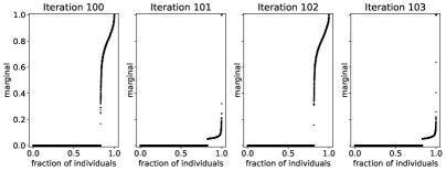
This parallel updates mechanism was tried out experimentally in [14]. However, this method does not converge. Instead, the messages oscillate between odd and even rounds as shown in Figure 8. Similar oscillations emerge in other applications of Belief Propagation. They may result from an instability of the empirical mean of the messages. To elaborate, if in some particular iteration the deviation from the prior
| (3.12) |
is positive, then we should expect a negative deviation in the next round. This is because due to (3.12) in the next iteration many tests will receive a relatively large indication from that one of their samples may be infected. The test will therefore send out “less urgent” messages to the other samples. Conversely, if (3.12) is negative, then in iteration we expect to see a positive deviation. Due to the analytic nature of the update rules (3.1)–(3.3) these oscillations do not dampen down but actually blow up, leading to oscillations between odd and even rounds. This observation led the authors of [14] to turn to the computationally more intensive Glauber dynamics algorithm.
But actually oscillations of this type have been observed in other problems as well and several ideas for tackling the problem are on the market. Perhaps the most organic solution, and the method to which we resort, is to update the messages in a randomised fashion rather than in parallel. Hence, starting from the initialisation , we apply (3.2)–(3.3) once to initialise the test-to-sample messages as well. Then at each time we choose an edge of randomly and also flip a fair coin. If the coin comes up heads we update the message according to (3.1). Otherwise we update according to (3.2)–(3.3). The random choices break the cycle of oscillations. We stop the fixed point iteration after a fixed number of steps. The precise choice of is guided by experiments but of course should be chosen large enough so that every message will likely get updated several times. We note that this update scheme does not impede practical matters from using our algorithm in a laboratory setting since it purely pertains to the computations behind the scene and does not impact how samples are split and combined.
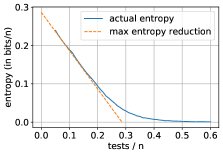
Beyond relying on asymptotic ideas and comparing the messages that result from the two aforementioned initialisations we take two additional steps to corroborate the results of Belief Propagation. First, we compared the marginals obtained by Belief Propagation with the empirical marginals of Glauber dynamics on a number of samples. They match. Second, we compared the marginals obtained via Belief Propagation on moderately sized biregular test designs with the marginal distributions obtained via population dynamics, a heuristic intended to approximate the limiting distribution of the marginals as [30]. Once again the Belief Propagation results align very well. Figure 9 displays the typical outcome of the Belief Propagation for different numbers of tests along with the estimate (3.9) of the remaining entropy.
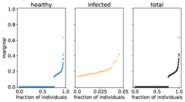
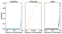
What conclusions are to be drawn regarding a promising test design? We see three different scenarios.
-
•
For small numbers of tests we can extract some information from the negative tests. For instance, in the case of perfect specificity we can rest assured that any sample included in a negative test is indeed uninfected. But beyond the direct effect of the negative tests the marginals do not align particularly well with the ground truth.
-
•
The second scenario concerns intermediate values of . Here Belief Propagation gains information from both positive and negative test results. As a consequence, the marginals start to align better with the ground truth.
-
•
Finally, once gets quite large the ground truth leaves a clear imprint on the test results. In this scenario we can recover the ground truth with good accuracy, albeit at the expense of investing many tests.
In light of what we learned on Belief Propagation, we now move on to describe the new adaptive Belief Propagation test design.
3.2. The first stage
As the first stage we use the random biregular design with the optimal choice of from (2.1) subject to rounding. Thus, the only free parameter is the total number of tests conducted in the first stage. Its choice is informed by Belief Propagation.
Specifically, we choose the largest number of tests up to which each test yields the optimal entropy reduction of . Practically, this means that we choose to match the point at which the entropy plot for the corresponding parameter values flattens. The fourth graphic in Figure 9 shows the approximation of the entropy as a function of the number of tests for our illustrative case of and in the noiseless setting. For other priors and noise levels, the story turns out to be analogous.
3.3. The second and third stage
Given the approximation of the marginals from the first stage, how should we proceed? As we saw in Section 2.3 and 2.5, two ideas for the subsequent stages proposed in the literature include individual testing of all samples whose marginals are not entirely polarised after the first round and informative Dorfman. The former strategy, known as Definite Defectives, seems wasteful as it completely disregards any non-trivial information about the marginals resulting from the Belief Propagation computation. The latter suffers from the same problem as the original Dorfman scheme, namely a potentially fairly large number of false positives and negatives.
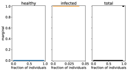
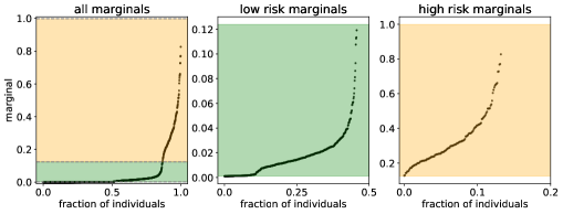
To remedy these issues, we propose a new design that blends the random biregular design with the informative Dorfman scheme from Section 2.5. For a start we threshold marginals obtained from the first stage at and . Thus, we report samples with Belief Propagation marginals less than as healthy and those with marginals beyond as infected right after the first stage. The remaining samples are split into two groups, one comprising samples with marginals below and one with marginals above. Let us refer to these as the low risk and the high risk groups, respectively. The choice of marks precisely the threshold beyond which the expressions (2.1) suggest that any sample should be placed in one test only. Figure 10 provides an illustration.
For the low risk group we set up another random biregular test design on which we run Belief Propagation once again. The posterior of the first stage now acts as the prior of the second stage. A range of different tests tested for the biregular test design depending on the prior, the posteriors of the first stage and noise level and the final recommended test numbers obtained via optimisation over this range. The resulting marginals are again thresholded at and . Those samples whose marginals fall in between are subsequently retested individually with their classification being solely determined by the outcome of the individual test.
To be more precise, let be the samples in the low risk group, let and let be the number of tests dedicated to this group. Thanks to the Belief Propagation results from the first stage we can (approximately) calculate the average marginal
Mimicing (2.1) we then choose the degrees
| (3.13) |
subject to rounding and set up a random biregular test design on . Furthermore, we modify the Belief Propagation equations on this random biregular design to accommodate the marginals computed in the first stage. Hence, instead of using the universal prior for all the samples, we substitute the separate marginals computed in the first stage:
| (3.14) |
The test-to-sample equations remain the same as in (3.2)–(3.3).
For the high risk group we set up an informative Dorfman design as described in Section 2.5. If such a pooled test turns out to be negative, we classify all samples in this pool as healthy. Otherwise, we conduct individual tests and classify samples solely based on this individual test result.
3.4. Enhanced accuracy
The construction that we described up to this point is the one labelled adaptive Belief Propagation 1 in Section 1.3. Enhanced constructions adaptive Belief Propagation 2 and adaptive Belief Propagation 3 further reduce the number of false positives and negatives, at the expense of increasing the number of tests. Indeed, the adaptive Belief Propagation 1 construction facilitates such enhancements explicitly. This is because almost all false positives and negatives actually originate from the informative Dorfman procedure in the second stage, while neither the thresholding nor the second-stage random biregular design tend to produce a notable number of mistakes. Therefore, in adaptive Belief Propagation 2 and adaptive Belief Propagation 3 we simply perform the informative Dorfman procedure twice or thrice independently in parallel. Thus, in adaptive Belief Propagation 2 and adaptive Belief Propagation 3 we double or triple the number of tests required for the informative Dorfman bit of the construction, but only for that bit.
If we perform informative Dorfman twice (adaptive Belief Propagation 2), we need to choose whether to reduce false negatives or false positives. Accordingly, we classify a sample as healthy (infected) if both Dorfman procedures classify it as healthy (infected). In adaptive Belief Propagation 3 we get to avoid both false positives and false negatives. To this end we classify according to the majority vote of the three informative Dorfman schemes. Table 1 illustrates the number of tests to be performed in the first and second stage depending on the prior and noise level.
| noiseless | moderate noise | high noise | |||||
|---|---|---|---|---|---|---|---|
| algorithm | prior | m1/n | c | m1/n | c | m1/n | c |
| Belief Propagation + individual testing | 0.5% | 0.05 | n/a | 0.09 | n/a | 0.11 | n/a |
| 1% | 0.08 | n/a | 0.12 | n/a | 0.16 | n/a | |
| 5% | 0.23 | n/a | 0.37 | n/a | 0.45 | n/a | |
| 10% | 0.3 | n/a | 0.7 | n/a | 0.34 | n/a | |
| Belief Propagation + informative Dorfman | 0.5% | 0.045 | n/a | 0.05 | n/a | 0.045 | n/a |
| 1% | 0.075 | n/a | 0.075 | n/a | 0.1 | n/a | |
| 5% | 0.28 | n/a | 0.24 | n/a | 0.16 | n/a | |
| 10% | 0.125 | n/a | 0.1 | n/a | 0.1 | n/a | |
| adaptive Belief Propagation (1x) | 0.5% | 0.035 | 1.0 | 0.05 | 2.0 | 0.05 | 2.0 |
| 1% | 0.075 | 1.0 | 0.085 | 2.0 | 0.1 | 2.0 | |
| 5% | 0.28 | 1.0 | 0.18 | 2.0 | 0.16 | 2.0 | |
| 10% | 0.125 | 0.25 | 0.15 | 4.0 | 0.1 | 2.0 | |
| adaptive Belief Propagation (2x) | 0.5% | n/a | n/a | 0.075 | 8.0 | 0.02 | 8.0 |
| 1% | n/a | n/a | 0.12 | 8.0 | 0.03 | 8.0 | |
| 5% | n/a | n/a | 0.4 | 2.0 | 0.36 | 2.0 | |
| 10% | n/a | n/a | 0.5 | 2.0 | 0.325 | 2.0 | |
| adaptive Belief Propagation (3x) | 0.5% | n/a | n/a | 0.075 | 8.0 | 0.02 | 8.0 |
| 1% | n/a | n/a | 0.085 | 8.0 | 0.03 | 8.0 | |
| 5% | n/a | n/a | 0.4 | 2.0 | 0.4 | 2.0 | |
| 10% | n/a | n/a | 0.55 | 2.0 | 0.5 | 2.0 | |
4. Asymptotic considerations
Clearly, adaptive Belief Propagation relies on heuristics and is not asymptotically optimal. This begs the question of how we would adapt the design and algorithm if we decide to live unburdened by practical considerations and consider the case ?
4.1. Variations on adaptive Belief Propagation
The optimal drop in entropy seen in Figure 9 shows that running Belief Propagation on a random biregular test design in the first stage seems like a good idea. The discrete partition into three groups in the second stage, however, gives something away. Indeed, in the asymptotic regime infinitesimal intervals of posterior marginals contain an unbounded number of samples.555Of course, depending on the prior and the noise setting the distribution of the posterior marginals need not be supported on the entire unit interval. Thus, it seems information-theoretically optimal to construct a random biregular design for every single small marginal interval and repeat this procedure over a few stages. However, such an approach does not seem practical since for moderate each random biregular design would only contain very few samples.
A simpler alternative that we considered is to still include all samples in one single second-stage test design, in which we choose the number of tests in which each sample takes part according to the posterior marginal from the first stage. Specifically, we chose these numbers so that in expectation half the tests should be positive. However, this design turned out to be unstable for small values of because of random fluctuations.
4.2. Plain Belief Propagation
Thus far we disregarded what might seem at first glance the most straightforward scheme: just run Belief Propagation on a random biregular design and then simply threshold the marginals at, say, . An obvious plus of this approach is that it requires one stage only. Indeed, when we simulated this scheme for large group testing instances such as , this approach turned out to work extremely well. Particularly for small priors such as and , the plain Belief Propagation plus thresholding design is on par or even outperforms adaptive Belief Propagation in terms of both efficiency and reliability. However, for smaller values of plain Belief Propagation plus threshold turns out to be extremely vulnerable to fluctuations of the number of infected samples. This is because such fluctuations might cause the fraction of positive tests to significantly deviate from half.
4.3. Scale effects
All the simulation results were presented for group testing instances with . However, we might be interested in smaller instances of say or larger ones such as . We performed extensive simulations in these directions and found that our results, particularly the power of the adaptive Belief Propagation scheme carry over to those group testing sizes as well, subject to rounding issues and few samples in a second stage for small instances necessitating slightly more tests.
4.4. Population dynamics
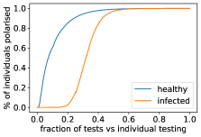
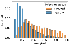
In the light of these scaling results for different instance sizes, let us spare a few more lines on the population dynamics already touched upon above. As mentioned above, this heuristic allows us to get a glimpse of the marginal distribution resulting from running Belief Propagation as [30]. To this end, we require as input the distribution of infected and healthy samples in the local neighbourhood of a sample which is provided in [23]. Subsequently, we iteratively sample the local neighbourhood for infected and healthy samples and perform one-step Belief Propagation updates to model the marginal distribution of those samples whose marginal is not completely polarised. The resulting distribution which is shown in Figure 11 for a prior of and the noiseless setting for illustration purposes closely resembles the marginal distribution that we observe from running Belief Propagation in our simulation in the first stage. As a side product, we obtain the proportion of polarised healthy and infected samples which lines up nicely with our simulation results. It should be noted that the population dynamics heuristic is nowhere near a complete analysis of Belief Propagation on random biregular graphs. Given the gains in efficiency and reliability that we observe in this empirical work for moderately-sized instances, a formal analysis of Belief Propagation seems to be an important next step in group testing research.
5. Discussion
Group testing is a powerful method to efficiently and accurately detect infected samples. Since the mathematical work on group testing deals with the asymptotic scenario, practical adoption of methods proposed in this literature has been limited. Instead practitioners tend to apply very simple test designs dating back to the 1940s. In this paper we therefore conducted an experimental study that shows how a mildly more sophisticated test design can significantly improve the accuracy of the overall test results by comparison to classical methods without asking for many more tests. The new test design comes with an efficient, easy-to-run and easy-to-implement algorithm that determines the status of each sample from the test results. Since the new design employs randomisation, its adoption is probably feasible only in a practical setting that employs a degree of automation in preparing test pools. But on the plus side the new adaptive Belief Propagation design keeps the pool sizes and the number of pools that each sample has to be placed in fairly low.
Apart from the group testing model studied in the present paper, there are several other, more complicated models. For example, in quantitative group testing each test returns the number of infected samples rather than a binary positive or negative result. Further variants include the pooled data problem, the generalised coin weighing problem or the compressed sensing problem [17, 20].
What are the loose ends of the present work? On the one hand, it seems worthwhile to consider alternative noise models. A candidate might be one where the specificity decreases in the test size. Both the fixed noise model considered in this work and this diluted model have value from a practical perspective and it would be interesting to see whether our results carry over. On the other hand, the success of Belief Propagation in practical group testing leaves us wondering whether it is guaranteed to converge to a fixed point reminiscent of the ground truth. Hence, a mathematical analysis of Belief Propagation remains as an outstanding open problem.
Acknowledgement
The authors thank Oliver Johnson for his helpful comments on group testing algorithms.
References
- [1] M. Aldridge, Individual testing is optimal for nonadaptive group testing in the linear regime, IEEE Transactions on Information Theory, 65 (2019), pp. 2058–2061, https://doi.org/10.1109/TIT.2018.2873136.
- [2] M. Aldridge, Conservative two-stage group testing, 2020, https://arxiv.org/abs/2005.06617.
- [3] M. Aldridge, L. Baldassini, and O. Johnson, Group testing algorithms: Bounds and simulations, IEEE Transactions on Information Theory, 60 (2014), pp. 3671–3687, https://doi.org/10.1109/TIT.2014.2314472.
- [4] M. Aldridge, O. Johnson, and J. Scarlett, Group Testing: An Information Theory Perspective, Foundations and Trends in Communications and Information Theory, 2019.
- [5] V. Bapst and A. Coja-Oghlan, Harnessing the bethe free energy, Random Structures & Algorithms, 49 (2016), pp. 694–741, https://doi.org/10.1002/rsa.20692.
- [6] J. Barbier and D. Panchenko, Strong replica symmetry in high-dimensional optimal bayesian inference, 2020, https://arxiv.org/abs/2005.03115.
- [7] V. Brault, B. Mallein, and J.-F. Rupprecht, Group testing as a strategy for COVID-19 epidemiological monitoring and community surveillance, PLOS Computational Biology, 17 (2021), p. e1008726, https://doi.org/10.1371/journal.pcbi.1008726.
- [8] A. N. Cohen, B. Kessel, and M. G. Milgroom, Diagnosing SARS-CoV-2 infection: the danger of over-reliance on positive test results, Cold Spring Harbor Laboratory, (2020), https://doi.org/10.1101/2020.04.26.20080911.
- [9] A. Coja-Oghlan, C. Efthymiou, N. Jaafari, M. Kang, and T. Kapetanopoulos, Charting the replica symmetric phase, Communications in Mathematical Physics, 359 (2018), pp. 603–698, https://doi.org/10.1007/s00220-018-3096-x.
- [10] A. Coja-Oghlan, O. Gebhard, M. Hahn-Klimroth, and P. Loick, Information-theoretic and algorithmic thresholds for group testing, IEEE Transactions on Information Theory, 66 (2020), pp. 7911–7928, https://doi.org/10.1109/TIT.2020.3023377.
- [11] A. Coja-Oghlan, O. Gebhard, M. Hahn-Klimroth, and P. Loick, Optimal group testing, Combinatorics, Probability and Computing, (2021), pp. 1–38, https://doi.org/10.1017/s096354832100002x.
- [12] A. Coja-Oghlan and W. Perkins, Belief propagation on replica symmetric random factor graph models, Annales de l’Institut Henri Poincaré D, 5 (2018), pp. 211–249, https://doi.org/10.4171/aihpd/53.
- [13] A. Coja-Oghlan and W. Perkins, Bethe states of random factor graphs, Communications in Mathematical Physics, 366 (2019), pp. 173–201, https://doi.org/10.1007/s00220-019-03387-7.
- [14] M. Cuturi, O. Teboul, Q. Berthet, A. Doucet, and J.-P. Vert, Noisy adaptive group testing using bayesian sequential experimental design, 2020, https://arxiv.org/abs/2004.12508.
- [15] D. Donoho, Compressed sensing, IEEE Transactions on Information Theory, 52 (2006), pp. 1289–1306, https://doi.org/10.1109/TIT.2006.871582.
- [16] D. L. Donoho, A. Javanmard, and A. Montanari, Information-theoretically optimal compressed sensing via spatial coupling and approximate message passing, IEEE Transactions on Information Theory, 59 (2013), pp. 7434–7464, https://doi.org/10.1109/TIT.2013.2274513.
- [17] D. L. Donoho, A. Maleki, and A. Montanari, Message-passing algorithms for compressed sensing, Proceedings of the National Academy of Sciences, 106 (2009), pp. 18914–18919, https://doi.org/10.1073/pnas.0909892106.
- [18] R. Dorfman, The detection of defective members of large populations, The Annals of Mathematical Statistics, 14 (1943), pp. 436–440, https://doi.org/10.1214/aoms/1177731363.
- [19] C. Efthymiou, T. P. Hayes, D. Štefankovič, E. Vigoda, and Y. Yin, Convergence of MCMC and loopy BP in the tree uniqueness region for the hard-core model, SIAM Journal on Computing, 48 (2019), pp. 581–643, https://doi.org/10.1137/17m1127144.
- [20] A. El Alaoui, A. Ramdas, F. Krzakala, L. Zdeborová, and M. I. Jordan, Decoding from pooled data: Phase transitions of message passing, IEEE Transactions on Information Theory, 65 (2019), pp. 572–585, https://doi.org/10.1109/TIT.2018.2855698.
- [21] A. Frieze and M. Karonski, Introduction to Random Graphs, Cambridge University Press, 2015, https://doi.org/10.1017/cbo9781316339831.
- [22] L. P. Garrison, J. B. Babigumira, A. Masaquel, B. C. Wang, D. Lalla, and M. Brammer, The lifetime economic burden of inaccurate HER2 testing: Estimating the costs of false-positive and false-negative HER2 test results in US patients with early-stage breast cancer, Value in Health, 18 (2015), pp. 541–546, https://doi.org/10.1016/j.jval.2015.01.012.
- [23] O. Gebhard and P. Loick, Note on the offspring distribution for group testing in the linear regime, 2021, https://arxiv.org/abs/2103.13039.
- [24] E. Joly and B. Mallein, Group testing and pcr: a tale of charge value, 2020, https://arxiv.org/abs/2012.09096.
- [25] S. Kleinman, D. Strong, G. Tegtmeier, P. Holland, J. Gorlin, C. Cousins, R. Chiacchierini, and L. Pietrelli, Hepatitis b virus (HBV) DNA screening of blood donations in minipools with the COBAS AmpliScreen HBV test, Transfusion, 45 (2005), pp. 1247–1257, https://doi.org/10.1111/j.1537-2995.2005.00198.x.
- [26] F. Krzakala, M. Mézard, F. Sausset, Y. F. Sun, and L. Zdeborová, Statistical-physics-based reconstruction in compressed sensing, Phys. Rev. X, 2 (2012), p. 021005, https://doi.org/10.1103/PhysRevX.2.021005.
- [27] D. A. Levin and Y. Peres, Markov Chains and Mixing Times (Second Edition), American Mathematical Society, 2017.
- [28] S. Mallapaty, The mathematical strategy that could transform coronavirus testing, Nature, 583 (2020), pp. 504–505, https://doi.org/10.1038/d41586-020-02053-6.
- [29] C. S. McMahan, J. M. Tebbs, and C. R. Bilder, Informative dorfman screening, Biometrics, 68 (2011), pp. 287–296, https://doi.org/10.1111/j.1541-0420.2011.01644.x.
- [30] M. Mézard and A. Montanari, Information, Physics, and Computation, Oxford University Press, Inc., 2009, https://doi.org/10.5555/1592967.
- [31] M. Müller, P. M. Derlet, C. Mudry, and G. Aeppli, Testing of asymptomatic individuals for fast feedback-control of COVID-19 pandemic, Physical Biology, 17 (2020), p. 065007, https://doi.org/10.1088/1478-3975/aba6d0.
- [32] Y. Ohhashi, A. Pai, H. Halait, and R. Ziermann, Analytical and clinical performance evaluation of the cobas TaqScreen MPX test for use on the cobas s 201 system, Journal of Virological Methods, 165 (2010), pp. 246–253, https://doi.org/10.1016/j.jviromet.2010.02.004.
- [33] J. Pearl, Probabilistic Reasoning in Intelligent Systems, Elsevier, 1988, https://doi.org/10.1016/c2009-0-27609-4.
- [34] T. Richardson and R. Urbanke, Modern Coding Theory, Cambridge University Press, 2008, https://doi.org/10.1017/cbo9780511791338.
- [35] N. Shental, S. Levy, V. Wuvshet, S. Skorniakov, B. Shalem, A. Ottolenghi, Y. Greenshpan, R. Steinberg, A. Edri, R. Gillis, M. Goldhirsh, K. Moscovici, S. Sachren, L. M. Friedman, L. Nesher, Y. Shemer-Avni, A. Porgador, and T. Hertz, Efficient high-throughput SARS-CoV-2 testing to detect asymptomatic carriers, Science Advances, 6 (2020), p. eabc5961, https://doi.org/10.1126/sciadv.abc5961.
- [36] M. Sherlock, N. M. Zetola, and J. D. Klausner, Routine detection of acute HIV infection through RNA pooling: Survey of current practice in the united states, Sexually Transmitted Diseases, 34 (2007), pp. 314–316, https://doi.org/10.1097/01.olq.0000263262.00273.9c.
- [37] J. M. Tebbs, C. S. McMahan, and C. R. Bilder, Two-stage hierarchical group testing for multiple infections with application to the infertility prevention project, Biometrics, 69 (2013), pp. 1064–1073, https://doi.org/10.1111/biom.12080.
- [38] L. N. Theagarajan, Group testing for covid-19: How to stop worrying and test more, 2020, https://arxiv.org/abs/2004.06306.
- [39] G. U. van Zyl, W. Preiser, S. Potschka, A. T. Lundershausen, R. Haubrich, and D. Smith, Pooling strategies to reduce the cost of HIV-1 RNA load monitoring in a resource-limited setting, Clinical Infectious Diseases, 52 (2010), pp. 264–270, https://doi.org/10.1093/cid/ciq084.
- [40] P. O. Vontobel, Counting in graph covers: A combinatorial characterization of the bethe entropy function, IEEE Transactions on Information Theory, 59 (2013), pp. 6018–6048, https://doi.org/10.1109/TIT.2013.2264715.
- [41] J. Watson, P. F. Whiting, and J. E. Brush, Interpreting a covid-19 test result, BMJ, (2020), p. m1808, https://doi.org/10.1136/bmj.m1808.
- [42] L. Zdeborová and F. Krzakala, Statistical physics of inference: thresholds and algorithms, Advances in Physics, 65 (2016), pp. 453–552, https://doi.org/10.1080/00018732.2016.1211393.
Appendix A Sample splits and test degree
The algorithms required the following number of maximum test degree and the following maximum and average split of samples. The algorithms can be readily adjusted to work with smaller test degrees or sample splits at the expense of slightly more tests.
| noiseless | moderate noise | high noise | ||||||||
|---|---|---|---|---|---|---|---|---|---|---|
| algorithm | prior | |||||||||
| Belief Propagation + individual testing | 0.5% | 140 | 8 | 7.0 | 134 | 13 | 12.0 | 137 | 16 | 15.0 |
| 1% | 75 | 7 | 6.0 | 67 | 9 | 8.0 | 69 | 12 | 11.0 | |
| 5% | 14 | 4 | 3.1 | 14 | 6 | 5.2 | 14 | 7 | 6.2 | |
| 10% | 7 | 3 | 2.3 | 8 | 6 | 5.2 | 6 | 3 | 2.8 | |
| Belief Propagation + informative Dorfman | 0.5% | 134 | 8 | 6.0 | 140 | 9 | 7.1 | 134 | 8 | 6.2 |
| 1% | 67 | 7 | 5.1 | 67 | 7 | 5.2 | 70 | 9 | 7.2 | |
| 5% | 15 | 6 | 4.1 | 20 | 5 | 3.5 | 13 | 4 | 2.9 | |
| 10% | 8 | 3 | 1.8 | 14 | 3 | 2.3 | 10 | 3 | 2.3 | |
| adaptive Belief Propagation | 0.5% | 143 | 8 | 5.2 | 140 | 11 | 7.6 | 140 | 13 | 8.0 |
| 1% | 67 | 8 | 5.1 | 71 | 12 | 6.7 | 70 | 13 | 8.0 | |
| 5% | 15 | 7 | 4.1 | 147 | 12 | 6.2 | 66 | 12 | 6.5 | |
| 10% | 8 | 3 | 1.8 | 172 | 19 | 10.3 | 50 | 10 | 4.9 | |
Appendix B Distribution between stages
Based on the number of tests in the first and second stage, the following table shows the fraction of samples identified in each round. It evinces that despite a total of three stages needed for adaptive Belief Propagation the majority of samples are identified already in the first and second stage, depending on the prior and noise level.