Anomalous diffusion and Lévy walks distinguish active from inertial turbulence

Abstract

Bacterial swarms display intriguing dynamical states like active turbulence. Using a hydrodynamic model we now show that such dense active suspensions manifest super-diffusion, via Lévy walks, which masquerades as a crossover from ballistic to diffusive scaling in measurements of mean-squared-displacements, and is tied to the emergence of hitherto undetected oscillatory streaks in the flow. Thus, while laying the theoretical framework of an emergent advantageous strategy in the collective behaviour of microorganisms, our study underlines the essential differences between active and inertial turbulence.

Flowing active matter, resulting from the motility of organisms, cells and particles, forms an intriguing class of non-equilibrium phenomena [Marchetti et al., 2013; Ramaswamy, 2017; Doostmohammadi et al., 2018]. Biological functions like foraging and evasion, that require active agents to both sample their neighbourhoods and make large jumps to cover ground, become inextricably coupled with collective flow patterns in dense systems [Shellard and Mayor, 2020]. Active flow driven enhanced diffusion and mixing are also essential for feeding of microorganisms [Humphries, 2009; Leptos et al., 2009; Lagarde et al., 2020]. Active agents, hence, profit from optimal processes like Lévy motion [Humphries et al., 2010; Volpe and Volpe, 2017; Shlesinger and Klafter, 1986] characterised by long-tailed, self-similar step-size distributions leading to anomalous diffusion [Klafter and Sokolov, 2005] and increased encounter rates [Bartumeus et al., 2002] — all which can emerge from simple generative mechanisms [Reynolds, 2015]—as opposed to inefficient meandering by random walks limited to classical diffusion. Interestingly, the motion of individual active entities in isolation often differ from when they are in large numbers [Knebel et al., 2021]: Movements of a single swimming bacteria can be fundamentally different from its motion in a dense, fluid-like swarm Ariel et al. [2015].

A remarkable feature of the collective behaviour of dense active suspensions is the emergence of spatio-temporal structures strongly reminiscent of inertial turbulence [Dombrowski et al., 2004; Wensink et al., 2012; Dunkel et al., 2013a; Zhou et al., 2014; Wu et al., 2017; Martínez-Prat et al., 2019]: Such two-dimensional suspensions are vortical [Giomi, 2015], chaotic [Wensink et al., 2012] with non-Gaussian distributions of velocity gradients [Giomi, 2015; James et al., 2018; James and Wilczek, 2018] and a power-law kinetic energy spectrum [Bratanov et al., 2015; Alert et al., 2020]. These facets of low Reynolds number suspensions have led to a new class of phenomena known as active turbulence [Alert et al., 2021].

However, does the similarity between high Reynolds number inertial turbulence and low Reynolds number active turbulence hold even for Lagrangian statistics? This is a fundamentally important question for two reasons. First, while for inertial turbulence, Lagrangian (tracer) trajectories, measured through mean squared displacements (MSD) have a universal behaviour of purely diffusive self-separation [Xia et al., 2013], experiments in active turbulence suggest non-universal signatures of Lévy walks and anomalous diffusion [Wu and Libchaber, 2000; Kurtuldu et al., 2011; Morozov and Marenduzzo, 2014; Ariel et al., 2015]. Secondly, if such effective biological strategies emerge in active suspensions, why have they remained theoretically undetected and experimentally inconclusive so far?

Using a continuum hydrodynamic model we now provide definitive answers to these questions. We show what appears as an inconsequential transition (see Fig. 1(a)) between the ballistic and diffusive scaling regimes in MSD measurements is really an intermediate, anomalous diffusive regime leveraging the crucial biological advantages of Lévy walks [Kanazawa et al., 2020]. Thus, while low Reynolds number active suspensions may well share features, at the level of equations and the resultant dynamics, with high Reynolds number inertial turbulence, active turbulence still allows for emergent behaviour consistent with biological systems striving for efficient searching strategies. This, we discover, is facilitated by a synthesis of two basic flow patterns: Novel oscillatory streaks responsible for anomalous diffusion and unique to such systems, and vortical features reminiscent of inertial turbulence.

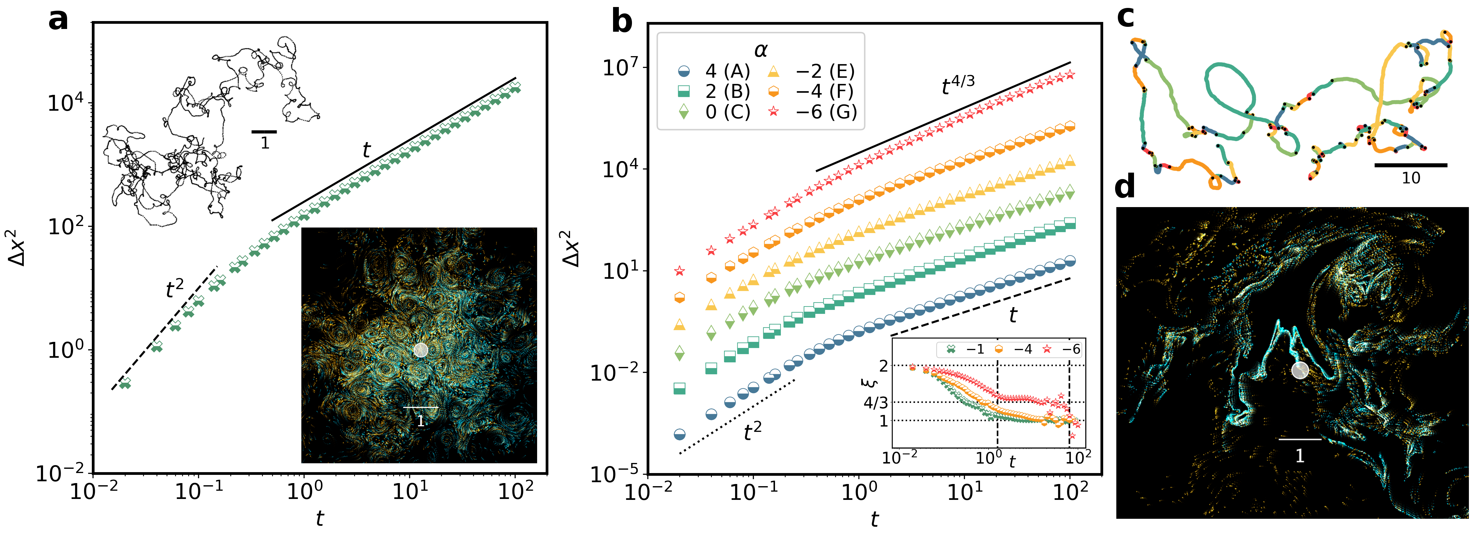
Figure 1: MSD of Lagrangian trajectories (a) for mild activity and (b) with increasing levels of activity (vertically staggered for clarity). Local slopes (b, inset) of $\Delta x^{2}$: While $\xi$ continuously decreases from $2$ to $1$ for $\alpha\leq-4$, it plateaus (between the vertical lines) at $\xi\approx 4/3$ for $\alpha=-6$. Representative trajectories for (a) $\alpha=-1$ (upper inset) and (c) $\alpha=-6$ (see text) reflecting the change from diffusive to anomalous behaviour and also seen in snapshots of particle positions (initially localised within the small white disk) at $t\approx 10$ for $\alpha=-1$ (panel (a), lower inset) and (d) $\alpha=-6$; the brightness of the colours reflects the particle density (see movie at https://youtu.be/w3V_cQdvC2k).

Dense, active suspensions lend themselves to a generalized hydrodynamic description, developed for bacterial swarms Wensink et al. [2012]; Dunkel et al. [2013b]

$$\partial_{t}{\bf u}+\lambda{\bf u}\cdot\nabla{\bf u}=-\nabla p-\Gamma_{0}\nabla^{2}{\bf u}-\Gamma_{2}\nabla^{4}{\bf u}-(\alpha+\beta|{\bf u}|^{2}){\bf u}$$ (1)

where the incompressible velocity field ${\bf u}({\bf x},t)$ (with $\nabla\cdot\bf u=0$), is a coarse-grained description of the motility of dense, active (bacterial) suspensions. Here, $\lambda>0$ corresponds to pusher-type bacteria and the $\Gamma-$terms are responsible for quasi-chaotic pattern formation via stress-induced instabilities (when $\Gamma_{0},\Gamma_{2}>0$) in the bacterial system [Swift and Hohenberg, 1977; Wensink et al., 2012; Simha and Ramaswamy, 2002; Linkmann et al., 2020; Bratanov et al., 2015]. The last term adds Toner-Tu drive [Toner and Tu, 1995, 1998], where $\beta$ needs to be positive for stability, while the activity $\alpha$ can take both positive (Ekman friction) and negative (active injection) values. In our direct numerical simulations (see Supplemental Material), $\Gamma_{0}$ and $\Gamma_{2}$ are fixed according to experimental length and time scales Wensink et al. [2012], while other parameters are varied to obtain the flow fields explored in this study. The characteristic length and time scales associated with the linear instability in (1) are $L_{\Gamma}=\sqrt{{\Gamma_{2}}/{\Gamma_{0}}}$ and $\tau_{\Gamma}={\Gamma_{2}}/{\Gamma_{0}^{2}}$ Wensink et al. [2012], while the activity length and time scales are given by $1/\sqrt{|\alpha|\beta}$ and $1/|\alpha|$, respectively. In conformity with the previous studies using this model, we present our results in simulation units.

Figure 1(a) shows the MSD $\Delta x^{2}=\left\langle{||\mathbf{x}(t)-\mathbf{x}(0)||^{2}}\right\rangle$ (where $||\cdot||$ and $\left\langle{\cdot}\right\rangle$ denote the Euclidean norm and ensemble averaging over all particles, respectively) for an active suspension with $\alpha=-1.0$. This scaling behaviour seems consistent with inertial turbulence: A ballistic regime $\Delta x^{2}\sim t^{2}$ crossing over to a diffusive regime $\Delta x^{2}\sim t$ [C.P. and Joy, 2020]. Individual trajectories (upper inset, Fig. 1(a)), similarly, show diffusive meandering.

However, some experiments [Wu and Libchaber, 2000; Ariel et al., 2015] on dense bacterial swarms provide strong evidence of anomalous diffusion $\Delta x^{2}\sim t^{\xi}$, with $1<\xi<2$. This raises the question whether what is seen as a crossover from ballistic to diffusive behaviour is actually masking an intermediate, anomalous diffusive regime.

To uncover the true behaviour of such suspensions, we perform several simulations on domain sizes $20\leq L\leq 80$ with $-6\leq\alpha\leq 4$, seeded with tracers that evolve as $\mathrm{d}\mathbf{x}(t)/\mathrm{d}t=\mathbf{u}(\mathbf{x},t)$, and measure the associated MSD as shown in Fig. 1(b). For $\alpha\geq 0$, corresponding to an Ekman friction effect, and for modest activity $0<\alpha\leq-2$ (Cases A – E), we see little evidence of anomalous diffusion. However, as we increase the activity further (Case F), the first signatures of an intermediate regime appear. This observation is validated for Case G where the $\Delta x^{2}$ shows a convincing super-diffusive regime, and local slope analysis (Fig. 1(b), inset) gives $\xi=\frac{d{\rm Log}\Delta x^{2}}{d{\rm Log}t}=1.31\pm 0.08\approx 4/3$, for close to two decades before giving way to diffusion. This scaling, we recall, is not inconsistent with recent experimental measurements [Wu and Libchaber, 2000; Ariel et al., 2015] and simplified model predictions [Ariel et al., 2017; Ariel and Schiff, 2020] which suggest similar super-diffusion for dense suspensions of motile bacteria. It is important to alert the reader that whether these are indeed non-trivial fixed points in the renormalisation group sense would require an exponent flow [Panja et al., 2015] or more sophisticated data analysis through asymptotic extrapolation van der Hoeven [2009]; Pauls and Frisch [2007]; Bardos et al. [2010]; Chakraborty et al. [2012]; given the high precision data required for such approaches to be beyond speculative, we refrain from this analysis here.

The emergence of anomalous diffusion, as suspensions become more active, ought to carry its signature in Lagrangian trajectories, providing a crucial link in understanding how bacterial colonies forage and avoid hostile environments. In Fig. 1(c) we show a representative trajectory of a tracer corresponding to a highly active suspension with $\alpha=-6$ which, in sharp contrast to trajectories in mildly active suspensions (Fig. 1(a), upper inset), shows short diffusive behaviour punctuated by long “steps” indicative of anomalous diffusion. This is clearly illustrated in the movies of trajectories for different activities (see https://youtu.be/G97ndUVeNRQ).

Figure 1(c) shows a trajectory divided into segments (shown in different colours), that are identified every time the trajectory turns (points marked in black) by an angle $\theta$ greater than a threshold angle $\theta_{c}$; we choose $\theta_{c}=30^{\circ}$ for illustration in Fig. 1(c). While trajectories evolve mostly with small variations in $\theta$ for mild suspensions, increasing activity makes sharper turns more probable (see Supplemental Material).

The changing nature of particle trajectories and transition from normal to anomalous diffusion is also reflected in the spreading of an initially localised puff of particles (see https://youtu.be/w3V_cQdvC2k). In Fig. 1(d) we show a snapshot of 20,000 particles, initially localised within the small white disk at the center, at time $t\approx 10$ for Case G ($\alpha=-6$); the brightness of the colours is a measure of the local density of particles. The evolution of the puff in highly active suspensions is far more “irregular” than what is seen, under identical conditions, at low activity ($\alpha=-1$, Fig. 1(a), lower inset) where they spread through diffusion.

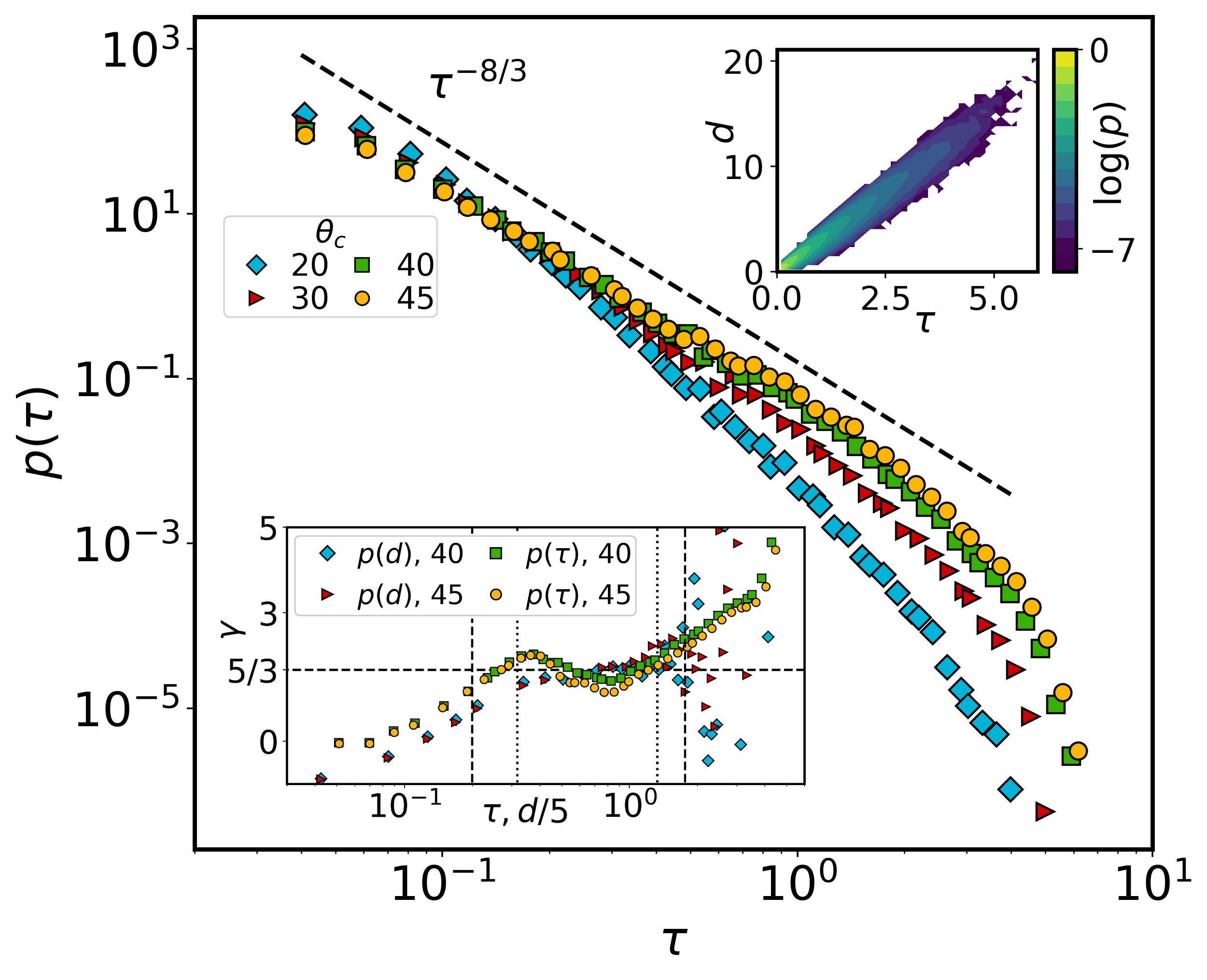
Figure 2: For highly active suspensions (Case G), probability distributions $p(\tau)$ of the waiting time $\tau$ with a $\tau^{-8/3}$ scaling (dashed line), as a guide to the eye, for different $\theta_{c}$. (Lower inset) Local slope analysis of $p(\tau)$ and $p(d)$ (x-axis rescaled for visualisation) yields $\gamma=1.7\pm 0.3$ and $\gamma=1.6\pm 0.2$, respectively, consistent with Lévy walk estimates, showing a scaling range (between dashed ($p(\tau)$) and dotted ($p(d)$) vertical lines) for about a decade. (Upper inset) Joint probability distribution of $d$ and $\tau$ confirming a finite velocity through the near linear relationship between the two.

This inevitably leads to the question whether these visual cues are stemming from real Lévy walks, marked by power-law step size and equivalently, because of an approximately constant velocity, waiting time distributions Shlesinger et al. [1987]. A convincing argument in favour of Lévy walks is the distribution $p(\tau)$ of waiting times $\tau$, which ought to show a significant range of scaling of the form $p(\tau)\sim\tau^{-\gamma-1}$ for a reasonably large spread in the choice of the threshold angle $\theta_{c}$ which determines a “turn”. Fig. 2 confirms the existence of such a power-law and a local slope analysis $\gamma=-1-\frac{d{\rm Log}p(\tau)}{d{\rm Log}\tau}$ (Fig. 2, lower inset) shows scaling for about a decade with $\gamma=1.7\pm 0.3$. Similarly, the probability distribution $p(d)$ of step sizes, for the more active suspensions, follow a scaling $p(d)\sim d^{-\gamma-1}$. Hence, in the same inset, we also show local slopes obtained from $p(d)$ (with the x-axis rescaled to $d/5$ for ease of comparison), showing a comparable extent of scaling, from which we obtain $\gamma=1.6\pm 0.2$. Importantly, this scaling exponent $\gamma\approx 5/3$ when coupled with the anomalous MSD exponent $\xi\approx 4/3$, satisfies the Lévy walk constraint $\gamma+\xi=3$ [Zaburdaev et al., 2015]. Finally, the joint distribution of flight lengths $d$ and waiting times $\tau$ between turns in the trajectories for active suspensions (Fig. 2, upper inset) shows an almost linear scaling reflecting a constant system velocity. All of these are clear, unambiguous indicators of Lévy walks foo .

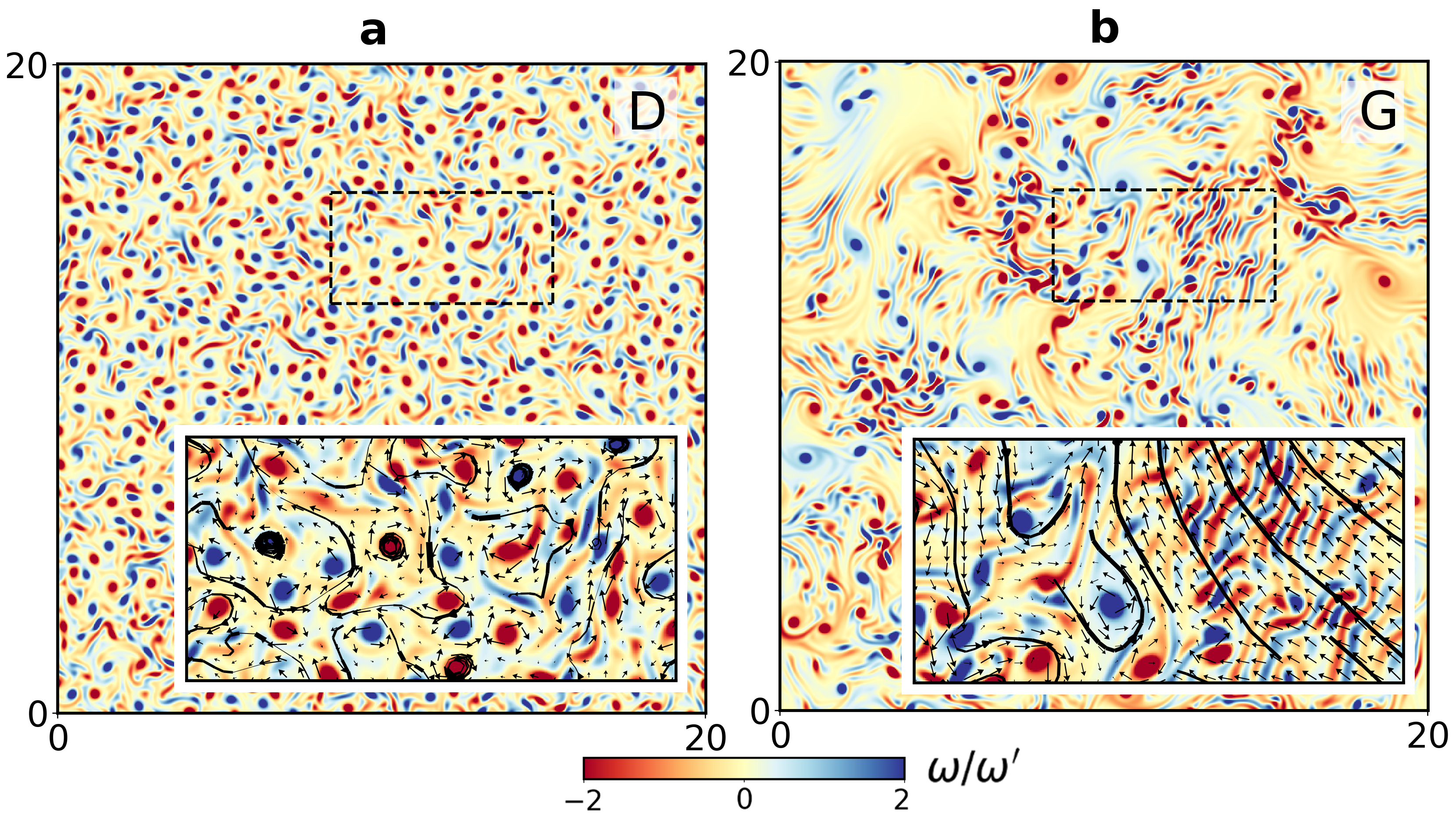
Figure 3: Representative snapshots of vorticity fields (and their magnified sections with velocity vectors as arrows and instantaneous streamlines as solid lines) for (a) Case D ($\alpha=-1$), and (b) Case G ($\alpha=-6$). In the latter, highly active suspensions a new feature shows up: The vorticity field is now populated by oscillatory streaks (see also Fig. 4 and https://youtu.be/gqhT-xf_tAc).

Does the emergence of (Lagrangian) anomalous scaling carry tell-tale signs in the vorticity field ${\boldsymbol{\omega}}=\nabla\times{\bf u}$? Figure 3 (see https://youtu.be/gqhT-xf_tAc for movies of evolving fields) shows slices of the vorticity field, for Cases D and G. While the vorticity fields appear, overall, disorganized—active turbulence—a closer inspection reveals a pattern hitherto undetected. With increasing activity, the dense packing of diffused vortices, which mainly appear as spots, gives way to sharper spots with trailing wisps of vorticity streaks (Case D). For highly active suspensions (Case G), there is an equal preponderance of spots and streaks. Curiously, these streaks appear with alternating signs in a periodic fashion with a characteristic length scale $\delta$.

The probability distribution of vorticity $p(\omega)$ is non-Gaussian (similarly to inertial turbulence) with fat tails which fall-off as a power-law, becoming more pronounced with increasing activity (see Supplemental Material). This analogy with inertial turbulence extends to the energy spectrum scaling as $k^{-5/3}$ scaling at high activity Pandit et al. [2009, 2017] (see Supplemental Material).

Is there a causal link between the alternating streaks and the anomalous diffusion that we observe? Careful measurements certainly suggest so. While a definitive answer is beyond the scope of this work, the instantaneous, jet-like velocity and elongated streamlines, orthogonal to the streaks, (Fig. 3 insets) would in the absence of dynamics ensure the persistence of trajectories, often over lengths $\mathcal{O}(L/2)$ (consistent with the scaling extent in $p(d)$), while the vortical patches serve to reorient trajectories. Naïvely, this suggests streak regions as origins of anomalous diffusion, while their absence (low activity) leads to classical diffusion. Importantly, these streaks are distinct from the “laning” phenomena in some active suspensions [Wensink and Löwen, 2012]. In order to further test the role of streaks, we push the system to an extreme case (with $\alpha=-16.66$ and $\beta=22.22$), which shows that the emergence of more distinct, pattern forming streaks (Fig. 4(a), with a magnified view in panel (b)) is accompanied by a robust super-diffusive $\Delta x^{2}\sim t^{4/3}$ regime (Fig. 4(c)). Unsurprisingly, the trajectories reflect this anomalous diffusion through clear Lévy walks (see inset in Fig. 4(c)), and are also found to have power-law distributions of $d$ and $\tau$. Thus, we show that active systems are actually super-diffusive and what may be mistaken as a cross-over from ballistic to diffusive behaviour masks the most important and non-trivial aspects of such systems.

While the origin of the oscillatory streaks remains to be established, it seems reasonable to assume that the length scale $\delta$, determining the alternating pattern of streaks, is influenced by the activity which sets the characteristic velocity for global polar ordering $v_{0}=\sqrt{|\alpha|/\beta}$ [Wensink et al., 2012]. Since the dominant time-scale is set by activity, $\delta\simeq 1/\sqrt{|\alpha|\beta}$. Given the heuristic nature of this argument, we made careful measurements of the “wavelength” of the oscillations for a range of parameters and found that they are in reasonable agreement with our conjectured estimate. Why the system senses this length scale will perhaps be found when the origins of these oscillatory streaks are systematically known, and the question of universality (or not) of such oscillatory patterns for different classes of active systems is an important one. While the specific model Chen et al. [2016] studied in this work seems to allow for an instability that triggers spatio-temporal chaotic states with bands of opposite polarities which show up as spots and streaks Maitra [2021], the precise mechanisms involved are left for future work.

Nature exploits Lévy movements and anomalous diffusion, across scales, ranging from the microscopic to ecological [Reynolds, 2018], and across taxa, from systems comprising individual agents like midge swarms Reynolds and Ouellette [2016], migrating metastatic cancer cells [Huda et al., 2018], living cancer cells Gal and Weihs [2010] and intracellular DNA transport [Muralidharan et al., 2021], foraging marine predators [Sims et al., 2008] and expanding colonies of seemingly immobile beach grasses [Reijers et al., 2019], to dense systems with collective flow states like swimming bacteria [Ariel et al., 2015]. Yet, detecting Lévy walks theoretically in active turbulence has remained elusive, despite some experimental results strongly suggestive of their existence. While recent work using a particle-based active model [Kanazawa et al., 2020] reconciles some of these findings, the lack of consistency with the most general hydrodynamic framework to describe active suspensions is surprising. We uncover why this is, showing that while it is true that anomalous diffusion is hardly detectable (though incipient in the light of our results) for mildly active suspensions, such systems exhibit distinct Lévy walks and super-diffusion when nudged to higher levels of activity.

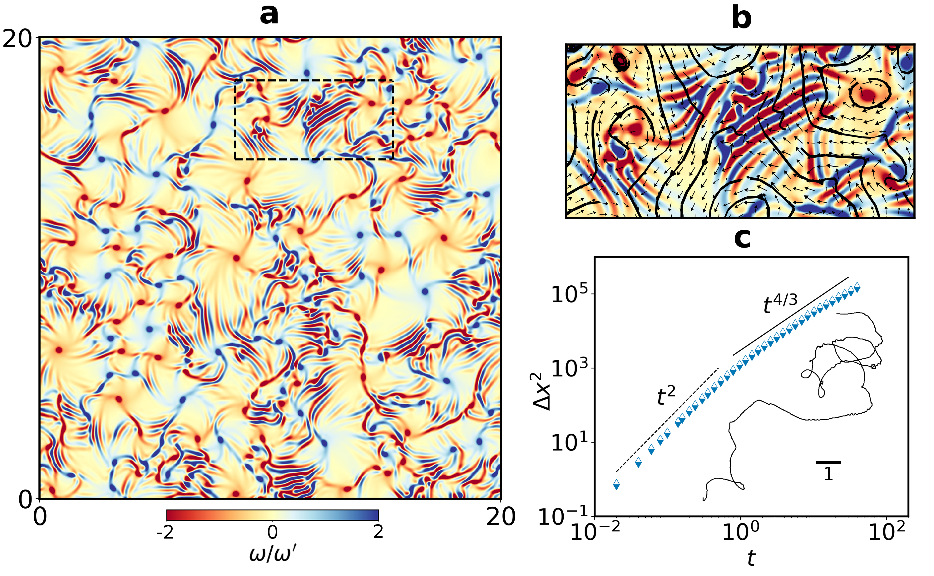
Figure 4: Extremely active suspensions shows that (a) the vorticity field is dominated by streaks interspersed with fewer vortical spots (magnified view in panel (b) with velocity vectors as arrows and instantaneous streamlines as solid lines) and is associated with (c) robust anomalous diffusion $\Delta x^{2}\sim t^{4/3}$, reflected in a representative trajectory (inset).

Our observations of the vorticity spots and streaks, a basis of future theories of emergent anomalous diffusion, provide a template for clearly identifiable structures experimentally. Thus experiments would be able to probe how universal these patterns are, aiding a more robust understanding of why they emerge and whether they are central to the super-diffusive behaviour of such systems. Recent works, which derive the hydrodynamic model presented here from microswimmer dynamics, show that the activity is related, among other factors, to their individual motility Heidenreich et al. [2016]; Reinken et al. [2018]. Thus high activity might be achieved by tuning the motility. A potential candidate for an experiment is a spermatozoa suspension James et al. [2020], which also exhibit a turbulent phase Creppy et al. [2015] and whose motility can be controlled by changing the ambient temperature Alavi and Cosson [2005].

Finally, we underline what sets active turbulence apart from inertial fluid turbulence and thus the limitations of drawing equivalences between the two. The Lagrangian picture, arising from our work, marks a crucial departure in the analogy in a rather counter-intuitive way. This is because for Eulerian statistics, increasing activity results in a more intermittent vorticity field and accompanying power-laws of energy spectra (see Supplemental Material) like in two-dimensional fluid turbulence. However, this “increasingly turbulent state” in active systems is paradoxically accompanied by persistent super-diffusion, Lévy walks and structural changes in the vorticity field which have no known counterparts in inertial turbulence. It would be interesting, however, to see how this distinction manifests itself in other measurements such as pair-particle dispersion [Boffetta and Celani, 2000].

Before concluding, we recall that our MSD exponent $\xi\approx 4/3$ (at high activity) is consistent with those predicted for 1D Hamiltonian systems Spohn [2014]. Whether this suggests a possible underlying universality is unclear. Recent theoretical studies of the walk time distribution Miron [2020a, b] show that local dynamics are central to super-diffusion with $\gamma=3/2$. While we detect $\gamma\approx 5/3$, it is possible that this exponent is one of an intermediate asymptotics (in $\alpha$) which may converge to $3/2$ for sufficiently high activity and diffusive behaviour appears as a pre-asymptotic correction to the asymptotic super-diffusive regime Miron [2021] that we report.

Our work suggests that activity is geared for manifesting optimality: Yet another way biological systems continue to defy bounds on inanimate matter, now in a turbulence-like flow state. This gives new direction to the assessment of what is truly turbulent, and universal, in low Reynolds number active flows.

Supplemental Material

Direct Numerical Simulations

The generalized hydrodynamic model, is solved using a pseudo-spectral method [James and Wilczek, 2018]. Simulations are performed on a periodic domain of sizes $1024^{2}$ and $4096^{3}$ grid points, with a physical extent of $L=20$ and $L=80$, respectively, for a duration of $5\times 10^{5}$ iterations, with a time-step of $\delta t=0.0002$. To be consistent with previous work [Wensink et al., 2012; James and Wilczek, 2018; C.P. and Joy, 2020], we set $\Gamma_{0}=0.045$, $\Gamma_{2}=\Gamma_{0}^{3}$, $\beta=0.5$, $\lambda=3.5$. Cases A to G correspond to $\alpha\in\left\{4,2,0,-1,-2,-4,-6\right\}$. We additionally simulate Case Z, after a parameter search, with $\beta=22.22$ and $\alpha=-16.66$, which is to exemplify an extreme state dominated by streaks, leading to robust anomalous diffusion.

After a spinup period of $2\times 10^{4}$ iterations, the flow is seeded with $10^{5}$ tracer particles randomly distributed in the domain, which follow the equation $\mathrm{d}\mathbf{x}(t)/\mathrm{d}t=\mathbf{u}(\mathbf{x},t)$ Perlekar et al. [2011]; Ray et al. [2011], integrated with a 4th-order Runge-Kutta scheme. Field quantities are interpolated to off-grid locations using bilinear interpolation, and data is stored every $100$ iterations to report well-converged statistics.

Quantifying Trajectories

Each trajectory is divided into individual walking segments (as illustrated in the main text) that are identified by a threshold on the turning angle $\theta$ at each time $t$. The angles $\theta(t)$ are calculated along trajectories as

$$\cos\left(\theta(t)\right)=\frac{\Delta\mathbf{r}(t)\cdot\Delta\mathbf{r}(t+\Delta t)}{|\Delta\mathbf{r}(t)||\Delta\mathbf{r}(t+\Delta t)|}$$ (2)

where $\Delta\mathbf{r}(t^{\prime})$ is the displacement vector connecting points $\mathbf{r}(t^{\prime}-\Delta t)$ and $\mathbf{r}(t^{\prime})$, and $\Delta t$ is the temporal coarsening, and results were found similar for $\Delta t=2\delta t,3\delta t$ and $4\delta t$. Individual segments and turns can be identified using a simple threshold of $\theta(t)>\theta_{c}$, although the exact segments are rather sensitive to the choice of $\theta_{c}$. A filtering is done to identify clusters of two or three successive points that are all identified as “turns” (usually occurs during sharp turns), where only the point with the highest turning angle is retained. The waiting time $\tau$ is calculated as the time between successive turns.

Supplemental Figures

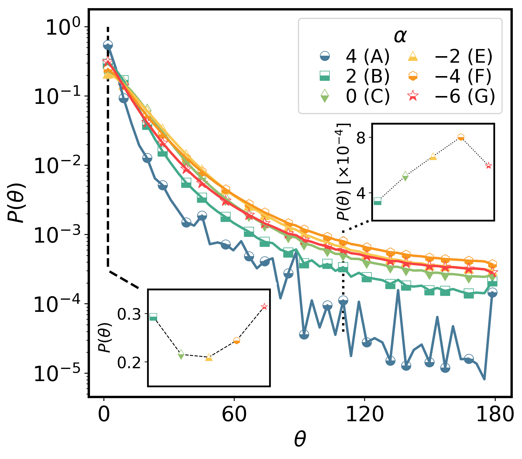
Figure 5: Distribution of turning angles. The probability distributions $P(\theta)$ along trajectories show that activity increases the probability of sharper turns. Moreover, the propensity for small changes in $\theta$ (Case A) first decreases with activity (up to Case E), and then increases again (Cases F and G), which, together with the prevalence of sharp turns at higher activity, reflects Lévy walk-like behaviour.

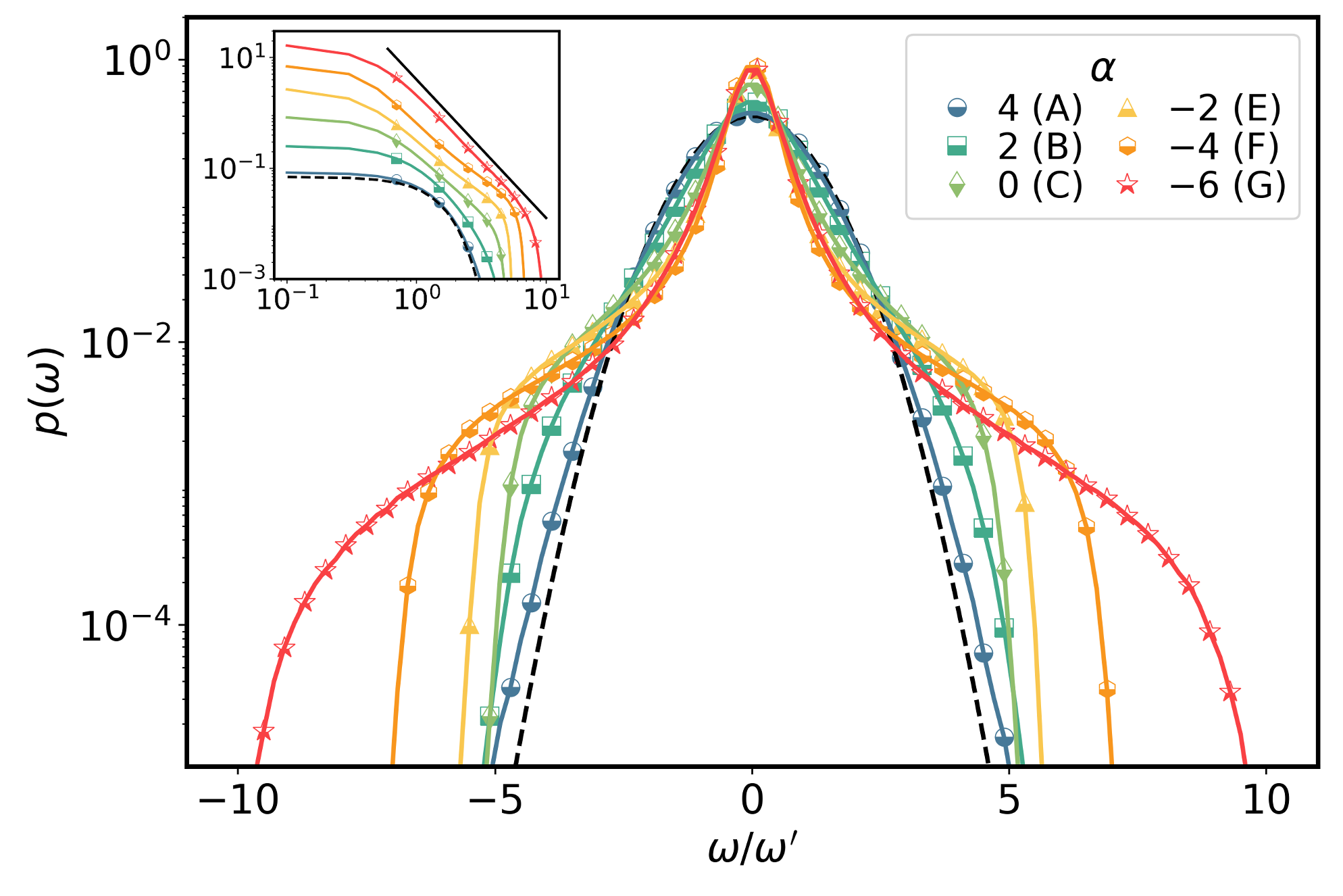
Figure 6: Vorticity distribution. The statistics of the $\boldsymbol{\omega}$ field is quantified by the probability density function $p(\omega)$ and it shows non-Gaussian, fat tails with power-laws (see inset, where the curves have been vertically staggered for clarity) as suspensions become more active. This increasing intermittency with higher activity is analogous to the effect of increasing Reynolds number in inertial turbulence.

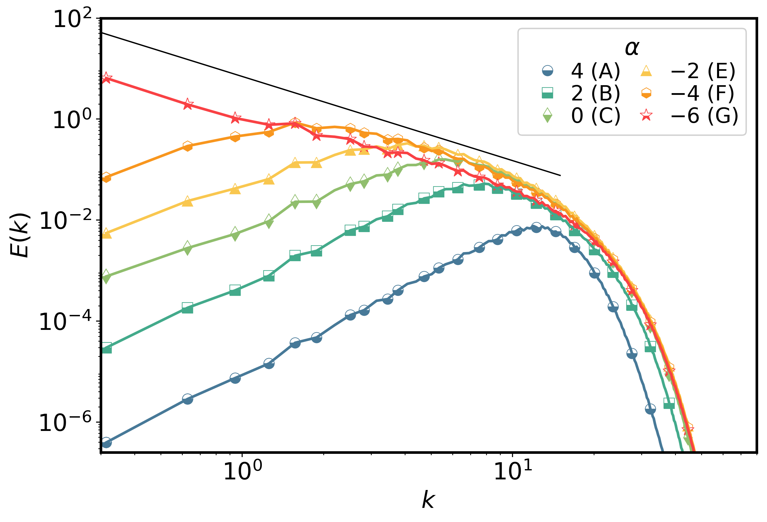
Figure 7: Energy spectra. The kinetic energy spectrum $E(k)$ asymptotically approaches a $k^{-5/3}$ power-law as the level of activity becomes high, which is again analogous to the energy spectrum in high Reynolds number inertial turbulence with an inverse-cascade.

References

- Marchetti et al. [2013] M. C. Marchetti, J.-F. Joanny, S. Ramaswamy, T. B. Liverpool, J. Prost, M. Rao, and R. A. Simha, Reviews of Modern Physics 85, 1143 (2013).
- Ramaswamy [2017] S. Ramaswamy, Journal of Statistical Mechanics: Theory and Experiment 2017, 054002 (2017).
- Doostmohammadi et al. [2018] A. Doostmohammadi, J. Ignés-Mullol, J. M. Yeomans, and F. Sagués, Nature communications 9, 1 (2018).
- Shellard and Mayor [2020] A. Shellard and R. Mayor, Philosophical Transactions of the Royal Society B 375, 20190387 (2020).
- Humphries [2009] S. Humphries, Proceedings of the National Academy of Sciences 106, 7882 (2009).
- Leptos et al. [2009] K. C. Leptos, J. S. Guasto, J. P. Gollub, A. I. Pesci, and R. E. Goldstein, Physical Review Letters 103, 198103 (2009).
- Lagarde et al. [2020] A. Lagarde, N. Dagès, T. Nemoto, V. Démery, D. Bartolo, and T. Gibaud, Soft Matter 16, 7503 (2020).
- Humphries et al. [2010] N. E. Humphries, N. Queiroz, J. R. Dyer, N. G. Pade, M. K. Musyl, K. M. Schaefer, D. W. Fuller, J. M. Brunnschweiler, T. K. Doyle, J. D. Houghton, et al., Nature 465, 1066 (2010).
- Volpe and Volpe [2017] G. Volpe and G. Volpe, Proceedings of the National Academy of Sciences 114, 11350 (2017).
- Shlesinger and Klafter [1986] M. F. Shlesinger and J. Klafter, in On growth and form (Springer, 1986) pp. 279–283.
- Klafter and Sokolov [2005] J. Klafter and I. M. Sokolov, Physics world 18, 29 (2005).
- Bartumeus et al. [2002] F. Bartumeus, J. Catalan, U. Fulco, M. Lyra, and G. Viswanathan, Physical Review Letters 88, 097901 (2002).
- Reynolds [2015] A. Reynolds, Physics of life reviews 14, 59 (2015).
- Knebel et al. [2021] D. Knebel, C. Sha-Ked, N. Agmon, G. Ariel, and A. Ayali, Iscience 24, 102299 (2021).
- Ariel et al. [2015] G. Ariel, A. Rabani, S. Benisty, J. D. Partridge, R. M. Harshey, and A. Be’Er, Nature communications 6, 1 (2015).
- Dombrowski et al. [2004] C. Dombrowski, L. Cisneros, S. Chatkaew, R. E. Goldstein, and J. O. Kessler, Physical review letters 93, 098103 (2004).
- Wensink et al. [2012] H. H. Wensink, J. Dunkel, S. Heidenreich, K. Drescher, R. E. Goldstein, H. Löwen, and J. M. Yeomans, Proceedings of the National Academy of Sciences 109, 14308 (2012).
- Dunkel et al. [2013a] J. Dunkel, S. Heidenreich, K. Drescher, H. H. Wensink, M. Bär, and R. E. Goldstein, Physical review letters 110, 228102 (2013a).
- Zhou et al. [2014] S. Zhou, A. Sokolov, O. D. Lavrentovich, and I. S. Aranson, Proceedings of the National Academy of Sciences 111, 1265 (2014).
- Wu et al. [2017] K.-T. Wu, J. B. Hishamunda, D. T. Chen, S. J. DeCamp, Y.-W. Chang, A. Fernández-Nieves, S. Fraden, and Z. Dogic, Science 355 (2017), 10.1126/science.aal1979.
- Martínez-Prat et al. [2019] B. Martínez-Prat, J. Ignés-Mullol, J. Casademunt, and F. Sagués, Nature Physics 15, 362 (2019).
- Giomi [2015] L. Giomi, Physical Review X 5, 031003 (2015).
- James et al. [2018] M. James, W. J. Bos, and M. Wilczek, Physical Review Fluids 3, 061101 (2018).
- James and Wilczek [2018] M. James and M. Wilczek, The European Physical Journal E 41, 1 (2018).
- Bratanov et al. [2015] V. Bratanov, F. Jenko, and E. Frey, Proceedings of the National Academy of Sciences 112, 15048 (2015).
- Alert et al. [2020] R. Alert, J.-F. Joanny, and J. Casademunt, Nature Physics 16, 682 (2020).
- Alert et al. [2021] R. Alert, J. Casademunt, and J.-F. Joanny, arXiv preprint arXiv:2104.02122 (2021), 2104.02122 .
- Xia et al. [2013] H. Xia, N. Francois, H. Punzmann, and M. Shats, Nature communications 4, 1 (2013).
- Wu and Libchaber [2000] X.-L. Wu and A. Libchaber, Physical review letters 84, 3017 (2000).
- Kurtuldu et al. [2011] H. Kurtuldu, J. S. Guasto, K. A. Johnson, and J. P. Gollub, Proceedings of the National Academy of Sciences 108, 10391 (2011).
- Morozov and Marenduzzo [2014] A. Morozov and D. Marenduzzo, Soft Matter 10, 2748 (2014).
- Kanazawa et al. [2020] K. Kanazawa, T. G. Sano, A. Cairoli, and A. Baule, Nature 579, 364 (2020).
- Dunkel et al. [2013b] J. Dunkel, S. Heidenreich, M. Bär, and R. E. Goldstein, New Journal of Physics 15, 045016 (2013b).
- Swift and Hohenberg [1977] J. Swift and P. C. Hohenberg, Physical Review A 15, 319 (1977).
- Simha and Ramaswamy [2002] R. A. Simha and S. Ramaswamy, Physical review letters 89, 058101 (2002).
- Linkmann et al. [2020] M. Linkmann, M. C. Marchetti, G. Boffetta, and B. Eckhardt, Physical Review E 101, 022609 (2020).
- Toner and Tu [1995] J. Toner and Y. Tu, Phys. Rev. Lett. 75, 4326 (1995).
- Toner and Tu [1998] J. Toner and Y. Tu, Phys. Rev. E 58, 4828 (1998).
- C.P. and Joy [2020] S. C.P. and A. Joy, Physical Review Fluids 5, 024302 (2020).
- Ariel et al. [2017] G. Ariel, A. Be’er, and A. Reynolds, Physical review letters 118, 228102 (2017).
- Ariel and Schiff [2020] G. Ariel and J. Schiff, Physica D: Nonlinear Phenomena 411, 132584 (2020).
- Panja et al. [2015] D. Panja, G. T. Barkema, and R. C. Ball, Macromolecules 48, 1442 (2015).
- van der Hoeven [2009] J. van der Hoeven, Journal of Symbolic Computation 44, 1000 (2009).
- Pauls and Frisch [2007] W. Pauls and U. Frisch, J Stat Phys 127, 1095 (2007).
- Bardos et al. [2010] C. Bardos, U. Frisch, W. Pauls, S. S. Ray, and E. Titi, Commun. Math. Phys. 293, 519 (2010).
- Chakraborty et al. [2012] S. Chakraborty, U. Frisch, W. Pauls, and S. S. Ray, Phys. Rev. E 85, 015301 (2012).
- Shlesinger et al. [1987] M. F. Shlesinger, B. West, and J. Klafter, Physical Review Letters 58, 1100 (1987).
- Zaburdaev et al. [2015] V. Zaburdaev, S. Denisov, and J. Klafter, Reviews of Modern Physics 87, 483 (2015).
- [49] There are of course examples of more generalised Lévy walks, such as those seen in the anomalous diffusion of cold atoms in optical lattices, where this linear relation fails Kessler and Barkai [2012]; Barkai et al. [2014].
- Pandit et al. [2009] R. Pandit, P. Perlekar, and S. S. Ray, Pramana 73, 157 (2009).
- Pandit et al. [2017] R. Pandit, D. Banerjee, A. Bhatnagar, M. Brachet, A. Gupta, D. Mitra, N. Pal, P. Perlekar, S. S. Ray, V. Shukla, et al., Physics of fluids 29, 111112 (2017).
- Wensink and Löwen [2012] H. Wensink and H. Löwen, Journal of Physics: Condensed Matter 24, 464130 (2012).
- Chen et al. [2016] L. Chen, C. F. Lee, and J. Toner, Nature communications 7, 12215 (2016).
- Maitra [2021] A. Maitra, Private Communication (2021).
- Reynolds [2018] A. M. Reynolds, Biology open 7 (2018), 10.1242/bio.030106.
- Reynolds and Ouellette [2016] A. M. Reynolds and N. T. Ouellette, Scientific reports 6, 1 (2016).
- Huda et al. [2018] S. Huda, B. Weigelin, K. Wolf, K. V. Tretiakov, K. Polev, G. Wilk, M. Iwasa, F. S. Emami, J. W. Narojczyk, M. Banaszak, et al., Nature communications 9, 1 (2018).
- Gal and Weihs [2010] N. Gal and D. Weihs, Phys. Rev. E 81, 020903 (2010).
- Muralidharan et al. [2021] A. Muralidharan, H. Uitenbroek, and P. E. Boukany, bioRxiv (2021), 10.1101/2021.04.12.435513.
- Sims et al. [2008] D. W. Sims, E. J. Southall, N. E. Humphries, G. C. Hays, C. J. Bradshaw, J. W. Pitchford, A. James, M. Z. Ahmed, A. S. Brierley, M. A. Hindell, et al., Nature 451, 1098 (2008).
- Reijers et al. [2019] V. C. Reijers, K. Siteur, S. Hoeks, J. van Belzen, A. C. Borst, J. H. Heusinkveld, L. L. Govers, T. J. Bouma, L. P. Lamers, J. van de Koppel, et al., Nature communications 10, 1 (2019).
- Heidenreich et al. [2016] S. Heidenreich, J. Dunkel, S. H. Klapp, and M. Bär, Physical Review E 94, 020601 (2016).
- Reinken et al. [2018] H. Reinken, S. H. Klapp, M. Bär, and S. Heidenreich, Physical Review E 97, 022613 (2018).
- James et al. [2020] M. James, D. A. Suchla, J. Dunkel, and M. Wilczek, arXiv preprint arXiv:2005.06217 (2020), 2005.06217 .
- Creppy et al. [2015] A. Creppy, O. Praud, X. Druart, P. L. Kohnke, and F. Plouraboué, Physical Review E 92, 032722 (2015).
- Alavi and Cosson [2005] S. M. H. Alavi and J. Cosson, Cell biology international 29, 101 (2005).
- Boffetta and Celani [2000] G. Boffetta and A. Celani, Physica A: Statistical Mechanics and its Applications 280, 1 (2000).
- Spohn [2014] H. Spohn, J Stat Phys 154, 1191 (2014).
- Miron [2020a] A. Miron, Phys. Rev. Lett. 124, 140601 (2020a).
- Miron [2020b] A. Miron, Phys. Rev. Research 2, 032042 (2020b).
- Miron [2021] A. Miron, Private Communication (2021).
- Perlekar et al. [2011] P. Perlekar, S. S. Ray, D. Mitra, and R. Pandit, Physical review letters 106, 054501 (2011).
- Ray et al. [2011] S. S. Ray, D. Mitra, P. Perlekar, and R. Pandit, Phys. Rev. Lett. 107, 184503 (2011).
- Kessler and Barkai [2012] D. A. Kessler and E. Barkai, Phys. Rev. Lett. 108, 230602 (2012).
- Barkai et al. [2014] E. Barkai, E. Aghion, and D. A. Kessler, Phys. Rev. X 4, 021036 (2014).