Critical even unimodular lattices in the Gaussian core model

Abstract.

We consider even unimodular lattices which are critical for potential energy with respect to Gaussian potential functions in the manifold of lattices having point density $1$. All even unimodular lattices up to dimension $24$ are critical. We show how to determine the Morse index in these cases. While all these lattices are either local minima or saddle points, we find lattices in dimension $32$ which are local maxima. Also starting from dimension $32$ there are non-critical even unimodular lattices.

1. Introduction

Let $L\subseteq\mathbb{R}^{n}$ be an $n$-dimensional lattice (a discrete subgroup of $\mathbb{R}^{n}$ of full rank). Let $f:(0,\infty)\to\mathbb{R}$ be a nonnegative function, then the $f$-potential energy of $L$ is defined as

$$\mathcal{E}(f,L)=\sum_{x\in L\setminus\{0\}}f(\|x\|^{2}).$$

In this paper we are mainly interested in Gaussian potential functions $f_{\alpha}(r)=e^{-\alpha r}$ with $\alpha>0$. Point configurations which interact via such a Gaussian potential function are referred to as the Gaussian core model. They are natural physical systems (see [22]) and they are mathematically quite general. By Bernstein’s theorem (see [25, Theorem 12b, page 161]), Gaussian potential functions span the convex cone of completely monotonic functions ($C^{\infty}$-functions $f$ with $(-1)^{k}f^{(k)}\geq 0$ for all $k\in\mathbb{N}$) of squared Euclidean distance.

We are interested in a local analysis of the function $L\mapsto\mathcal{E}(f_{\alpha},L)$ when $L$ varies in the manifold of rank $n$ lattices having point density $1$, which means that the number of lattice points per unit volume equals $1$. In particular, we want to understand which even unimodular lattices are critical points in the Gaussian core model and which type they have.

Recall that a lattice $L$ is called unimodular if it coincides with its dual lattice, which is defined as

$$L^{*}=\{y\in\mathbb{R}^{n}:x\cdot y\in\mathbb{Z}\text{ for all }x\in L\},$$

where $x\cdot y$ denotes the standard inner product of $x,y\in\mathbb{R}^{n}$. The lattice $L$ is called even if for every lattice vector $x\in L$ the inner product $x\cdot x$ is an even integer. It is well-known that in a given dimension the number of even unimodular lattices is finite and that they exist only in dimensions which are divisible by $8$. Furthermore, dimensions $8$ and $24$ seem to be very special. Cohn, Kumar, Miller, Radchenko and Viazovska [2] proved that the $E_{8}$ root lattice in dimension $8$ and the Leech lattice $\Lambda_{24}$ in dimension $24$ are universally optimal point configurations in their dimensions. This means that they minimize $f$-potential energy for all point configurations having density $1$ in their dimensions (not only for lattices) and for all completely monotonic functions of squared Euclidean distance.

1.1. Structure of the paper and main results

In Section 5 we present our concrete results. Here we summarize the phenomena which occur.

1.1.1. Dimension 8

Section 5.1: In dimension $8$ the $E_{8}$ root lattice is the only even unimodular lattice in dimension $8$ as observed by Mordell [14]. It is universally optimal. In particular, it is a local minimum for $f_{\alpha}$-potential energy. This was first proved by Sarnak and Strömbergsson [19], see also Coulangeon [4].

1.1.2. Dimension 16

Section 5.2: In dimension $16$ there are two even unimodular lattices $D_{16}^{+}$ and $E_{8}\perp E_{8}$, first classified by Witt [26]. Both of them are critical and we show that $D_{16}^{+}$ is a local minimum for $f_{\alpha}$-potential energy whenever $\alpha$ is large enough and that $E_{8}\perp E_{8}$ is a saddle point whenever $\alpha$ is large enough. Our numerical computations strongly suggest that $E_{8}\perp E_{8}$ is a saddle point for all values of $\alpha$.

1.1.3. Dimension 24

Section 5.3: Apart from the universally optimal Leech lattice there are $23$ further even unimodular lattices in dimension $24$. They were first classified by Niemeier [16]. Again they are all critical. We show how to determine their Morse index. We always find either local minima or saddle points.

1.1.4. Dimension 32

Section 5.4: It is known that there are more than 80 millions even unimodular lattices in dimension $32$; cf. Serre [20]. A complete classification has not been achieved yet. We show that not all of them are critical. We also show that there exist local maxima for $f_{\alpha}$-potential energy. This existence of local maxima answers a question of Regev and Stephens-Davidowitz [17] which arose in their proof strategy of the reverse Minkowski theorem; see also the exposition [1] by Bost for a broad perspective. A similar phenomenon, a local maximum for the covering density of a lattice, was earlier found by Dutour Sikirić, Schürmann, and Vallentin [6].

1.1.5. Proof techniques

To prove these results we make use of the theory of lattices and codes, especially spherical designs, theta series with spherical coefficients, and root systems. We recall these tools in Section 2. In Section 3 we describe our strategy which is based on the explicit computation of the signature of the Hessian of the function $L\mapsto\mathcal{E}(f_{\alpha},L)$. To work out this strategy it is necessary to explicitly compute the eigenvalues of a symmetric matrix which is parametrized by root systems. This is done in Section 4.

2. Toolbox

In this section we introduce the tools we shall apply later in this paper. For more information we refer to the standard literature on lattices and codes, in particular to Conway and Sloane [3], Ebeling [7], Serre [20], Venkov [24], Nebe [15]. Readers familiar with lattices and codes might like to skip immediately to the next section.

2.1. Spherical designs

A finite set $X$ on the sphere of radius $r$ in $\mathbb{R}^{n}$ denoted by $S^{n-1}(r)$ is called a spherical $t$-design if

$$\int_{S^{n-1}(r)}p(x)\,dx=\frac{1}{|X|}\sum_{x\in X}p(x)$$

holds for every polynomial $p$ of degree up to $t$. Here we integrate with respect to the rotationally invariant probability measure on $S^{n-1}(r)$.

If $X$ forms a spherical $2$-design, then

(1) $$\sum_{x\in X}xx^{\sf T}=\frac{r^{2}|X|}{n}I_{n},$$

holds, where $I_{n}$ denotes the identity matrix with $n$ rows/columns.

A polynomial $p\in\mathbb{R}[x_{1},\ldots,x_{n}]$ is called harmonic if it vanishes under the Laplace operator

$$\Delta p=\sum_{i=1}^{n}\frac{\partial^{2}p}{\partial x_{i}^{2}}=0.$$

We denote the space of homogeneous harmonic polynomials of degree $k$ by $\operatorname{Harm}_{k}$. One can uniquely decompose every homogeneous polynomial $p$ of even degree $k$

(2) $$p(x)=p_{k}(x)+\|x\|^{2}p_{k-2}(x)+\|x\|^{4}p_{k-4}(x)+\cdots+\|x\|^{k}p_{0}(x)$$

with $p_{d}\in\operatorname{Harm}_{d}$ and $d=0,2,\ldots,k$.

We can characterize that $X$ is a spherical $t$-design by saying that the sum $\sum_{x\in X}p(x)$ vanishes for all homogeneous harmonic polynomials $p$ of degree $1,\ldots,t$.

In the following we shall need the following technical lemma.

Lemma 2.1.

Let $H$ be a symmetric matrix with trace zero. The homogeneous polynomial

$$p_{H}(x)=(x^{\sf T}Hx)^{2}=H[x]^{2}$$

of degree four decomposes as in (2)

$$p_{H}(x)=p_{H,4}(x)+\|x\|^{2}p_{H,2}(x)+\|x\|^{4}p_{H,0}(x)$$

with $p_{H,d}\in\operatorname{Harm}_{d}$ and

$$p_{H,4}(x)=p_{H}(x)-\|x\|^{2}\frac{4}{4+n}H^{2}[x]+\|x\|^{4}\frac{2}{(4+n)(2+n)}\operatorname{Tr}H^{2}$$

and

$$p_{H,0}(x)=\frac{2}{(2+n)n}\operatorname{Tr}H^{2}.$$

Proof.

As a consequence of Euler’s formula we have for a general harmonic polynomial $q\in\operatorname{Harm}_{d}$

$$\Delta\|x\|^{2}q=(4d+2n)q+\|x\|^{2}\Delta q=(4d+2n)q,$$

and inductively

(3) $$\Delta\|x\|^{2(k+1)}q=(k+1)(4k+4d+2n)\|x\|^{2k}q,$$

see for example [21, Lemma 3.5.3].

Using (2) we get

$$\begin{split}\Delta p_{H}\;=\;&\Delta p_{H,4}+(8+2n)p_{H,2}+\|x\|^{2}\Delta p_{H,2}+\Delta\|x\|^{4}p_{H,0}\\ =\;&(8+2n)p_{H,2}+2(4+2n)\|x\|^{2}p_{H,0}.\end{split}$$

Applying the Laplace operator another time yields

$$\Delta^{2}p_{H}=8n(n+2)p_{H,0}.$$

On the other hand, one can compute $\Delta^{2}p_{H}$ directly. We have

$$H[x]=\sum_{i=1}^{n}\sum_{j=1}^{n}H_{ij}x_{i}x_{j}$$

and therefore

$$\Delta H[x]=2\sum_{i=1}^{n}H_{ii}=2\operatorname{Tr}H.$$

Using the product formula for the Laplace operator and the symmetry of $H$ we get

$$\Delta p_{H}=\Delta H[x]^{2}=2(H[x]\Delta H[x]+\nabla H[x]\cdot\nabla H[x])=4(\operatorname{Tr}H)H[x]+8H^{2}[x].$$

Therefore

$$\Delta^{2}p_{H}=8(\operatorname{Tr}H)^{2}+16\operatorname{Tr}H^{2}$$

and so

$$p_{H,0}=\frac{2}{n(n+2)}\operatorname{Tr}H^{2},$$

where the last equation follows from $\operatorname{Tr}H=0$.

We already computed

$$\Delta\|x\|^{4}p_{H,0}=2(4+2n)\|x\|^{2}p_{H,0}=\frac{8}{n}\operatorname{Tr}H^{2}\|x\|^{2}.$$

Now we determine $p_{H,2}$ when $\operatorname{Tr}H=0$:

$$(8+2n)p_{H,2}=\Delta p_{H}-\|x\|^{2}\frac{8}{n}\operatorname{Tr}H^{2}=8H^{2}[x]-\|x\|^{2}\frac{8}{n}\operatorname{Tr}H^{2}.$$

Finally we get $p_{H,4}$:

$$p_{H,4}=p_{H}-\|x\|^{2}\frac{4}{4+n}H[x]^{2}+\|x\|^{4}\frac{2}{(4+n)(2+n)}\operatorname{Tr}H^{2}.\qed$$

2.2. Theta series with spherical coefficients

We will make use of theta series with spherical coefficients. Let $L\subseteq\mathbb{R}^{n}$ be an even unimodular lattice and let $p$ be a harmonic polynomial (sometimes also called spherical polynomial).

We define the theta series of $L$ with spherical coefficients given by $p$ by

$$\Theta_{L,p}(\tau)=\sum_{x\in L}p(x)e^{\pi i\tau\|x\|^{2}}=\sum_{x\in L}p(x)q^{\frac{1}{2}\|x\|^{2}},$$

where $\tau$ lies in the upper half plane $\{z\in\mathbb{C}:\Im(z)>0\}$ and where $q=e^{2\pi i\tau}$.

If $p=1$ we also write $\Theta_{L}$ instead of $\Theta_{L,p}$. For $r\geq 0$ we define

$$L(r^{2})=\{x\in L:x\cdot x=r^{2}\}.$$

The set $L(r^{2})$ is called a shell of $L$ if it is not empty. Then

$$\Theta_{L}(\tau)=\sum_{m=0}^{\infty}a_{m}q^{m}\quad\text{with}\quad a_{m}=|L(2m)|.$$

The theta series of $L$ is related to its $f_{\alpha}$-potential energy through

$$\mathcal{E}(f_{\alpha},L)=\Theta_{L}(\alpha i/\pi)-1.$$

Using the Poisson summation formula one sees that

$$\Theta_{L}(iy)=y^{-n/2}\Theta_{L^{*}}(i/y)\;\text{ for }\;y>0.$$

In particular, when $L=L^{*}$ it is sufficient to consider Gaussian potentials with $\alpha\geq\pi$.

If $p$ is a homogeneous harmonic polynomial of degree $k$, then $\Theta_{L,p}$ is a modular form (for the full modular group $\mathrm{SL}_{2}(\mathbb{Z})$) of weight $n/2+k$. When $k>1$ then $\Theta_{L,p}$ is a cusp form. We only need that modular forms form a graded ring which is isomorphic to the polynomial ring $\mathbb{C}[E_{4},E_{6}]$ in the (normalized) Eisenstein series

$$E_{4}(\tau)=1+240q+2160q^{2}+6720q^{3}+\cdots,$$

and

$$E_{6}(\tau)=1-504q-16632q^{2}-122976q^{3}-\cdots,$$

where the weight of the monomial $E_{4}^{\alpha}E_{6}^{\beta}$ is $4\alpha+6\beta$. Generally, the normalized Eisenstein series are given by

$$E_{k}(\tau)=1-\frac{2k}{B_{k}}\sum_{m=1}^{\infty}\sigma_{k-1}(m)q^{m}\quad\text{for }k\geq 4,$$

where $B_{k}$ is the $k$-th Bernoulli number and where $\sigma_{k-1}(m)=\sum_{d|m}d^{k-1}$ is the sum of the $(k-1)$-th powers of positive divisors of $m$. The space of cusp forms is a principal ideal of the polynomial ring $\mathbb{C}[E_{4},E_{6}]$ generated by the modular discriminant

$$\Delta=\frac{1}{1728}(E_{4}^{3}-E_{6}^{2})=0+q-24q^{2}+252q^{3}\pm\cdots,$$

which has weight $12$.

It is a standard fact that the cardinality $a_{m}=|L(2m)|$ of the shells is asymptotically bounded, when $m$ tends to infinity, by

$$a_{m}=-\frac{n}{B_{n/2}}\sigma_{n/2-1}(m)+O(m^{n/4}),$$

but in this paper we shall need a bound with explicit constants.

For this we we will use the following explicit bound by Jenkins and Rouse [11] which relies on Deligne’s proof of the Weil conjectures: Let $f(\tau)=\sum_{m=1}^{\infty}a_{m}q^{m}$ be a cusp form of weight $k$, let $\ell$ be the dimension of the space of cusp forms of weight $k$, then

(4) $$\begin{split}|a_{m}|\leq&\sqrt{\log(k)}\left(11\cdot\sqrt{\sum_{r=1}^{\ell}\frac{|a_{r}|^{2}}{r^{k-1}}}+\frac{e^{18.72}(41.41)^{k/2}}{k^{(k-1)/2}}\cdot\left|\sum_{r=1}^{\ell}a_{r}e^{-7.288r}\right|\right)\\ &\qquad\cdot\;d(m)m^{\frac{k-1}{2}},\end{split}$$

where $d(m)$ is the number of divisors of $m$.

The following simple estimate will be helpful several times.

Lemma 2.2.

For $j\geq k/(2\alpha)$ we have

(5) $$\sum_{m=j}^{\infty}m^{k}e^{-2\alpha m}\leq j^{k}e^{-2\alpha j}+(2\alpha)^{-(k+1)}\Gamma(k+1,2\alpha j),$$

where

$$\Gamma(s,x)=\int_{x}^{\infty}t^{s-1}e^{-t}dt$$

is the incomplete gamma function.

As for fixed $s$ and large $x$

$$\Gamma(s,x)\sim x^{s-1}e^{-x}\left(1+\frac{s-1}{x}+\frac{(s-1)(s-2)}{x^{2}}+\cdots\right)$$

we see that the left hand side of (5) tends to zero for large $\alpha$ and fixed $j$ and $k$.

Proof.

The function $m\mapsto m^{k}e^{-2\alpha m}$ is monotonically decreasing for $m\geq k/(2\alpha)$. So we can apply the integral test

$$\sum_{m=j}^{\infty}m^{k}e^{-2\alpha m}\leq j^{k}e^{-2\alpha j}+\int_{j}^{\infty}m^{k}e^{-2\alpha m}\,dm.$$

Now using the definition of the incomplete gamma function after a change of variables yields the lemma. ∎

2.3. Root systems

The shell $L(2)$ is called the root system of the even unimodular lattice $L$, its elements are called roots. Witt classified in 1941 the possible root systems: These are orthogonal direct sums of the irreducible root systems $A_{n}$ ($n\geq 1$), $D_{n}$ ($n\geq 4$), $E_{6}$, $E_{7}$ and $E_{8}$. The rank of a root system is the dimension of the vector space it spans. Let $e_{1},\ldots,e_{n+1}$ be the standard basis for $\mathbb{R}^{n+1}$. The root system $A_{n}$ is defined as

$$\{\pm(e_{i}-e_{j}):1\leq i<j\leq n+1\}.$$

The root system $A_{n}$ has rank $n$, but lies in $\mathbb{R}^{n+1}$. It spans the vector space $\mathbb{R}^{n+1}\cap\mathbb{R}(1,\ldots,1)^{\perp}\cong\mathbb{R}^{n}$. In the following we will consider $A_{n}$ as a subset in $\mathbb{R}^{n}$. The root system $D_{n}$ is defined as

$$D_{n}=\{\pm(e_{i}\pm e_{j}):1\leq i<j\leq n\}.$$

Furthermore

$$E_{8}=D_{8}\cup\left\{\frac{e_{1}\pm\dots\pm e_{8}}{2}\right\},$$

where we restrict the last set to all sums having an even number of minus signs, and

$$E_{7}=E_{8}\cap\mathbb{R}(e_{7}-e_{8})^{\perp}\quad\text{and}\quad E_{6}=E_{7}\cap\mathbb{R}(e_{6}-e_{7})^{\perp}.$$

All irreducible root systems form spherical $2$-designs, and we have even spherical $4$-designs for $A_{1}$, $A_{2}$, $D_{4}$, $E_{6}$, $E_{7}$, and $E_{8}$.

Let $R$ be a root system. Let $\sigma(x)=I_{n}-xx^{\sf T}$ be the reflection at the hyperplane perpendicular to $x$. For all $x,y\in R$ we have $\sigma(x)y\in R$, so that $R$ is invariant under the reflection $\sigma(x)$. The group $W(R)$ generated by all reflections $\sigma(x)$, with $x\in R$, is called Weyl group of the root system.

The Coxeter number $h$ of a root system $R$ with rank $n$ is defined as $|R|/n$, the number of roots per dimension. For a root $r\in R$ we denote by $n_{0}$ the number of roots $r^{\prime}\in R$ with $r\cdot r^{\prime}=0$ and by $n_{1}$ the number of roots $r^{\prime}\in R$ with $r\cdot r^{\prime}=1$. These numbers $n_{0}$, $n_{1}$ do not depend on $r$ when $R$ is irreducible.

We summarize some properties of the irreducible root systems in Table 1.

name	rank	$|R|$	$n_{0}$	$n_{1}$	$h$	$|W|$
$A_{n}$	$n\geq 1$	$n(n+1)$	$(n-1)(n-2)$	$2(n-1)$	$n+1$	$(n+1)!$
$D_{n}$	$n\geq 4$	$2n(n-1)$	$2(n^{2}-5n+7)$	$4(n-2)$	$2(n-1)$	$2^{n-1}n!$
$E_{6}$	$6$	$72$	$30$	$20$	$12$	$2^{7}3^{4}5$
$E_{7}$	$7$	$126$	$60$	$32$	$18$	$2^{10}3^{4}57$
$E_{8}$	$8$	$240$	$126$	$56$	$30$	$2^{14}3^{5}5^{2}7$

Table 1. Some properties of the irreducible root systems.

3. Strategy

We compute the gradient and Hessian of $L\mapsto\mathcal{E}(f_{\alpha},L)$ at even unimodular lattices. For this it is convenient to parametrize the manifold of rank $n$ lattices having point density $1$ by positive definite quadratic forms of determinant $1$.

The gradient and the Hessian of $\mathcal{E}(f_{\alpha},L)$ at $L$ were computed by Coulangeon and Schürmann [5, Lemma 3.2]. Let $H$ be a symmetric matrix having trace zero (lying in the tangent space of the identity matrix). We use the notation $H[x]=x^{\sf T}Hx$ and we equip the space of symmetric matrices $\mathcal{S}^{n}$ with the inner product $\langle A,B\rangle=\operatorname{Tr}(AB)$, where $A,B\in\mathcal{S}^{n}$. The gradient is given by

(6) $$\langle\nabla\mathcal{E}(f_{\alpha},L),H\rangle=-\alpha\sum_{x\in L\setminus\{0\}}H[x]e^{-\alpha\|x\|^{2}}.$$

Now a sufficient condition for $L$ being a critical point is that all shells of $L$ form spherical $2$-designs. Indeed, we group the sum in (6) according to shells, giving

$$\langle\nabla\mathcal{E}(f_{\alpha},L),H\rangle=-\alpha\sum_{r>0}e^{-\alpha r^{2}}\sum_{x\in L(r^{2})}H[x].$$

Then for $r>0$ every summand

$$\sum_{x\in L(r^{2})}H[x]=\left\langle H,\sum_{x\in L(r^{2})}xx^{\sf T}\right\rangle=\frac{r^{2}|X|}{n}\operatorname{Tr}(H)=0$$

vanishes because of (1) and because $H$ is traceless. Hence, $L$ is critical.

This sufficient condition is fulfilled for all even unimodular lattices in dimensions $8$, $16$, and $24$. This fact can be deduced from the theory of theta functions with spherical coefficients and modular forms as first observed by Venkov [23]. In dimension $32$ this is no longer fulfilled in general but we can identify cases where it is.

The Hessian is the quadratic form

(7) $$\nabla^{2}\mathcal{E}(f_{\alpha},L)[H]=\alpha\sum_{x\in L\setminus\{0\}}e^{-\alpha\|x\|^{2}}\left(\frac{\alpha}{2}H[x]^{2}-\frac{1}{2}H^{2}[x]\right).$$

Again grouping the sum according to shells we get

(8) $$\nabla^{2}\mathcal{E}(f_{\alpha},L)[H]=\alpha\sum_{r>0}e^{-\alpha r^{2}}\sum_{x\in L(r^{2})}\left(\frac{\alpha}{2}H[x]^{2}-\frac{1}{2}H^{2}[x]\right).$$

So it remains to determine the two sums

(9) $$\sum_{x\in L(r^{2})}H[x]^{2}\quad\text{and}\quad\sum_{x\in L(r^{2})}H^{2}[x].$$

The second sum is easy to compute when $L(r^{2})$ forms a spherical $2$-design. In this case we have by (1)

(10) $$\sum_{x\in L(r^{2})}H^{2}[x]=\left\langle H^{2},\sum_{x\in L(r^{2})}xx^{\sf T}\right\rangle=\langle H^{2},\frac{r^{2}|L(r^{2})|}{n}I_{n}\rangle=\frac{r^{2}|L(r^{2})|}{n}\operatorname{Tr}H^{2}.$$

The first sum is only easy to compute when $L(r^{2})$ forms even a spherical $4$-design. Then (see [4, Proposition 2.2] for the computation)

(11) $$\sum_{x\in L(r^{2})}H[x]^{2}=\frac{r^{4}|L(r^{2})|}{n(n+2)}2\operatorname{Tr}H^{2}.$$

Together, when all shells form spherical $4$-designs, the Hessian (7) simplifies to

(12) $$\nabla^{2}\mathcal{E}(f_{\alpha},L)[H]=\frac{\operatorname{Tr}H^{2}}{n(n+2)}\sum_{r>0}|L(r^{2})|\alpha r^{2}\left(\alpha r^{2}-(n/2+1)\right)e^{-\alpha r^{2}}.$$

Therefore, every $H$ with Frobenius norm $\langle H,H\rangle=\operatorname{Tr}H^{2}=1$ is mapped to the same value, which implies that all the eigenvalues of the Hessian coincide.

Sarnak and Strömbergsson [19], see also Coulangeon [4], showed that for $L=E_{8},\Lambda_{24}$ the Hessian $\nabla^{2}\mathcal{E}(f_{\alpha},L)[H]$ is positive for all $\alpha>0$ which implies that $E_{8},\Lambda_{24}$ are local minima among lattices, for all completely monotonic potential functions of squared Euclidean distance.

The case when all shells form spherical $2$-designs but not spherical $4$-designs requires substantially more work. This is our main technical contribution. Then the Hessian has more than only one eigenvalue. We determine these eigenvalues up to dimension $32$ by considering the root system of $L$, that is the shell $L(2)$. Here the quadratic form

(13) $$Q[H]=\sum_{x\in L(2)}H[x]^{2}$$

will play a crucial role.

Indeed, consider again the first sum $\sum_{x\in L(r^{2})}H[x]^{2}$ in (9). We decompose the polynomial $p_{H}(x)=H[x]^{2}$ into its harmonic components as in Lemma 2.1 and get

$$\sum_{x\in L(r^{2})}p_{H}(x)=\sum_{x\in L(r^{2})}p_{H,4}(x)+r^{2}\sum_{x\in L(r^{2})}p_{H,2}(x)+r^{4}\sum_{x\in L(r^{2})}p_{H,0}(x).$$

Here the first sum equals

$$\sum_{x\in L(r^{2})}p_{H,4}(x)=\sum_{x\in L(r^{2})}H[x]^{2}-r^{4}\frac{2}{(2+n)n}|L(r^{2})|\operatorname{Tr}H^{2},$$

where we used Lemma 2.1 and (10). The second sum vanishes because $L(r^{2})$ is a spherical $2$-design and the third summand equals

$$r^{4}\sum_{x\in L(r^{2})}p_{H,0}(x)=r^{4}\frac{2}{(2+n)n}|L(r^{2})|\operatorname{Tr}H^{2}.$$

We can use theta series with spherical coefficients to determine the first sum $\sum_{x\in L(r^{2})}p_{H,4}(x)$ explicitly: $\Theta_{L,p_{H,4}}$ is a cusp form of weight $n/2+4$. In dimension $16$, $24$, and $32$ there is (up to scalar multiplication) only one cusp form of weight $n/2+4$. This is, respectively, $\Delta$, $E_{4}\Delta$ and $E_{4}^{2}\Delta$. Their $q$-expansions $\sum_{m=0}^{\infty}b_{m}q^{m}$ all start by $0+1\cdot q$. Therefore, by equating coefficients,

$$\Theta_{L,p_{H,4}}(\tau)=\sum_{r>0}\sum_{x\in L(r^{2})}p_{H,4}(x)q^{\frac{1}{2}r^{2}}=c\sum_{m=0}^{\infty}b_{m}q^{m}$$

with

$$c=\sum_{x\in L(2)}H[x]^{2}-\frac{8}{(2+n)n}|L(2)|\operatorname{Tr}H^{2}.$$

For $r^{2}=2m$ it follows

$$\sum_{x\in L(r^{2})}H[x]^{2}=cb_{m}+4m^{2}\frac{2}{(2+n)n}|L(2m)|\operatorname{Tr}H^{2}.$$

Hence, we only need to compute the eigenvalues of (13) to determine the signature of the Hessian. When talking about eigenvalues of $Q$, we refer to the eigenvalues of the Gram matrix with entries $b_{Q}(G_{i},G_{j})$, where $b_{Q}:\mathcal{S}^{n}\times\mathcal{S}^{n}\to\mathbb{R}$ is the induced bilinear form

(14) $$b_{Q}(G,H)=\sum_{x\in L(2)}G[x]H[x]$$

and $(G_{i})$ is an orthonormal basis of the space $\mathcal{S}^{n}$ with respect to the inner product $\langle\cdot,\cdot\rangle$. If $H$ is an eigenvector with eigenvalue $\lambda$, we have

$$\sum_{x\in L(2)}H[x]^{2}=\lambda\operatorname{Tr}H^{2}.$$

Now let us put everything together.

Theorem 3.1.

Let $L$ be an even unimodular lattice in dimension $n\leq 32$. Let

$$\Theta_{L}(\tau)=\sum_{m=0}^{\infty}a_{m}q^{m}\quad\text{with $a_{m}=|L(2m)|$}$$

be the theta series of $L$ and let $\sum_{m=1}^{\infty}b_{m}q^{m}$ be the cusp form of weight $n/2+4$ with $b_{1}=1$. Then all the eigenvalues of the Hessian $\nabla^{2}\mathcal{E}(f_{\alpha},L)$ are given by

(15) $$\begin{split}&\frac{1}{n(n+2)}\sum_{m=1}^{\infty}\left(b_{m}\frac{\alpha^{2}}{2}(\lambda n(n+2)-8a_{1})\right)e^{-2\alpha m}\\ &\;+\;\frac{1}{n(n+2)}\sum_{m=1}^{\infty}\left(a_{m}2\alpha m\left(2\alpha m-(n/2+1)\right)\right)e^{-2\alpha m},\end{split}$$

where $\lambda$ is an eigenvalue of (13).

Note that this theorem also includes the case when all shells of $L$ form spherical $4$-designs like in (12) because of (11). In this case and when the parameter $\alpha$ is large enough, then (12) is strictly positive, which shows that $L$ is a local minimum for $f_{\alpha}$-potential energy.

Similarly, because the growth of $a_{m}$ and $b_{m}$ is polynomial in $m$ and because of the estimate provided in Lemma 2.2, we see that the first summand, $m=1$,

$$\frac{1}{n(n+2)}\left(\frac{\alpha^{2}}{2}(\lambda n(n+2))-2a_{1}\alpha(n/2+1)\right)e^{-2\alpha}$$

dominates (15) for large $\alpha$. In particular, for large $\alpha$, the first summand is strictly positive if $\lambda$ is strictly positive and the first summand is strictly negative if $\lambda$ vanishes and if $a_{1}\neq 0$. As the quadratic form (13) is a non-trivial sum of squares, the eigenvalues cannot be strictly negative and some eigenvalue is always strictly positive. From this consideration we get:

Corollary 3.2.

Let $L$ be an even unimodular lattice in dimension $n\leq 32$ which is critical for $f_{\alpha}$-potential energy. For all large enough $\alpha$ the lattice $L$ is a local minimum if and only if all eigenvalues of (13) are strictly positive. If one eigenvalue of (13) vanishes and if $|L(2)|>0$, then $L$ is a saddle point for all large enough $\alpha$.

4. Eigenvalues of (13)

In this section we shall compute the eigenvalues of the quadratic form (13) $Q[H]=\sum_{x\in R}H[x]^{2}$, where we write $R=L(2)$ for the root system of the lattice.

4.1. Irreducible root systems

First we consider the case when $R$ is an irreducible root system of type $A$, $D$, or $E$.

Theorem 4.1.

Let $R$ be an irreducible root system of type $A$, $D$, or $E$. The quadratic form $Q[H]=\sum_{x\in R}H[x]^{2}$ has the following eigenvalues:

root system	eigenvalue	multiplicity
$A_{n},~{}n\geq 1$	$4h=4(n+1)$	$1$
	$2(n+1)$	$n$, for $n\geq 2$
	$4$	$n(n-1)/2-1$, for $n\geq 2$
$D_{n},~{}n\geq 4$	$4h=8(n-1)$	$1$
	$4(n-2)$	$n-1$
	$8$	$n(n-1)/2$
$E_{6}$	$4h=48$	$1$
	$12$	$20$
$E_{7}$	$4h=72$	$1$
	$16$	$27$
$E_{8}$	$4h=120$	$1$
	$24$	$35$

We will embed the proof of Theorem 4.1 in the framework of representation theory. The Weyl group $W$ of the root system $R$ acts on the space of symmetric matrices $\mathcal{S}^{n}$ by conjugation

$$W\times\mathcal{S}^{n} \to\mathcal{S}^{n}$$

$$(S,H) \mapsto SHS^{\sf T}.$$

This turns $(\mathcal{S}^{n},\langle\cdot,\cdot\rangle)$ into a unitary representation of $W$, meaning that the action of $W$ preserves the inner product $\langle\cdot,\cdot\rangle$.

Then the bilinear form $b_{Q}$, defined in (14), is invariant under the action of the Weyl group $W$, that is $b_{Q}(SGS^{\sf T},SHS^{\sf T})=b_{Q}(G,H)$ for all $S\in W$. Due to the Riesz representation theorem, there is a linear map $T:\mathcal{S}^{n}\to\mathcal{S}^{n}$ such that

$$b_{Q}(G,H)=\langle G,T(H)\rangle$$

and the eigenvalues of the Gram matrix of $b_{Q}$ coincide with the eigenvalues of $T$. Since $b_{Q}$ is invariant under the action of $W$, the map $T$ commutes with the action of $W$, i.e.

(16) $$T(SHS^{\sf T})=ST(H)S^{\sf T}\quad\textup{ for all }S\in W,$$

hence, $T$ is intertwining the representation $(\mathcal{S}^{n},\langle\cdot,\cdot\rangle)$ of the Weyl group $W$ with itself.

Instead of only considering the specific map $T$ above, we determine the common eigenspaces of all intertwiners that intertwine the representation on $\mathcal{S}^{n}$ with itself. As these eigenspaces will turn out to be inequivalent, Schur’s lemma implies that these eigenspaces are exactly the pairwise orthogonal, irreducible, $W$-invariant subspaces of $\mathcal{S}^{n}$.

4.2. Peter-Weyl theorem for irreducible root systems

This gives rise to Theorem 4.2, which is a Peter-Weyl theorem for the representation $(\mathcal{S}^{n},\langle\cdot,\cdot\rangle)$ of the Weyl group $W$ of an irreducible root system.

To state the theorem, we need to fix some notation, based on the definition of root systems in Section 2.3. We consider $A_{n}$ as a root system in $\mathbb{R}^{n}$ and, by slight abuse of notation, we write $e_{i}-e_{j}$ for the corresponding root in $\mathbb{R}^{n}$. Moreover, define the symmetric bilinear operator $M:\mathbb{R}^{n}\times\mathbb{R}^{n}\rightarrow\mathcal{S}^{n}$ by

$$M(x,y)=xy^{\sf T}+yx^{\sf T}.$$

The action of the Weyl group on $M$ is given by

$$SM(x,y)S^{\sf T}=M(Sx,Sy),\qquad S\in W.$$

Furthermore, set

$$M(x)=\frac{1}{2}M(x,x)=xx^{\sf T}$$

and

$$P_{i}=\sum_{j\in\{1,\ldots,n+1\}\setminus\{i\}}M(e_{i}-e_{j})-2I_{n}.$$

Theorem 4.2 (Peter-Weyl for irreducible root systems).

The space of symmetric matrices can be decomposed into the following $W$-invariant, irreducible, inequivalent subspaces:

1. For $R=A_{n},~{}n\geq 2$

   $$\mathcal{S}^{n}=\operatorname{span}\{I_{n}\}\perp U_{1}(A_{n})\perp U_{2}(A_{n}),$$

   where

   $$U_{1}(A_{n}) =\operatorname{span}\{M(x,y):x,y\in A_{n},\,x\cdot y=0\},$$

   $$U_{2}(A_{n}) =\operatorname{span}\{P_{i}:i=1,\ldots,n+1\}.$$

2. For $R=D_{n},~{}n\geq 5$

   $$\mathcal{S}^{n}=\operatorname{span}\{I_{n}\}\perp U_{1}(D_{n})\perp U_{2}(D_{n}),$$

   where

   (17) $$U_{1}(D_{n})=\{M\in\mathcal{S}^{n}:M_{ii}=0,\,1\leq i\leq n\}.$$

   and

   (18) $$U_{2}(D_{n})=\{\textup{diag}(d_{1},\ldots,d_{n}):d_{1},\ldots,d_{n}\in\mathbb{R},\,d_{1}+\cdots+d_{n}=0\}.$$

   For $n=4$ the space $U_{1}(D_{4})$ further splits into two irreducible subspaces

   (19) $$\begin{split}U_{1}(D_{4})\;=\;&\left\{\begin{pmatrix}0&a&b&c\\ a&0&c&b\\ b&c&0&a\\ c&b&a&0\end{pmatrix}\,:\,a,b,c\in\mathbb{R}\right\}\\ &\perp\quad\left\{\begin{pmatrix}0&a&b&-c\\ a&0&c&-b\\ b&c&0&-a\\ -c&-b&-a&0\end{pmatrix}\,:\,a,b,c\in\mathbb{R}\right\}.\end{split}$$

3. For $R\in\{E_{6},E_{7},E_{8}\}$

   $$\mathcal{S}^{n}=\operatorname{span}\{I_{n}\}\perp\mathcal{T}^{n}_{0},$$

   where $\mathcal{T}^{n}_{0}$ is the space of traceless symmetric $n\times n$ matrices.

Remark 4.3.

The proofs of (i) and (ii) will be based on the representation theory of the symmetric group(see [8, Chapter 4] for details). In fact, the decompositions are immediate consequences of the representation theory of the symmetric group, most of the work lies in the explicit description of the irreducible subrepresentations, as we need these, for the explicit calculation of the eigenvalues in Theorem 4.1.

We will give an elementary proof of (iii) in Section 4.5. However, as one of the anonymous referees pointed out, this could also be done by computing the explicit characters of the representation, as it was already done in the literature. See [9] for the case $E_{6}$ and $E_{7}$, and [10], for the case $E_{8}$.

The main ingredient is a decomposition formula for a representation of $\mathfrak{S}_{n+1}$, the symmetric group on $n+1$ symbols. We write

$$U=\operatorname{span}\{e\},$$

where $e$ is the all ones vector, for the trivial representation and

(20) $$V_{n+1}=\left\{v\in\mathbb{R}^{n+1}\,:\,\sum_{i=1}^{n+1}v_{i}=0\right\}=U^{\perp}$$

for the standard representation of $\mathfrak{S}_{n+1}$. Clearly $U$ and $V_{n+1}$ are orthogonal as representations. Furthermore, both are irreducible: they are the cases of a standard principle to construct the irreducible representations of $\mathfrak{S}_{n+1}$ via Young symmetrizers, which give a one-to-one correspondence between partitions of $n+1$ and irreducible representations of $\mathfrak{S}_{n+1}$ [8, Theorem 4.3].

One then obtains the decomposition

(21) $$\operatorname{Sym}^{2}(V_{n+1})\cong U\oplus V_{n+1}\oplus V_{((n+1)-2,2)},$$

where $V_{((n+1)-2,2)}$ is another irreducible representation of $\mathfrak{S}_{n+1}$.

4.3. $A_{n}$

We will begin with (i). It is well known that $W(A_{n+1})\cong\mathfrak{S}_{n+1}$ and we can explicitly describe the action of $W(A_{n})$ in terms of the action of $\mathfrak{S}_{n+1}$ by permutation matrices via the identification $\mathcal{S}^{n}\cong\textup{Sym}^{2}(V_{n+1})$. For this, we explicitly write

$$\textup{Sym}^{2}(V_{n+1})=\{A\in\mathcal{S}^{n+1}\,:\,Ae=0\},$$

where, again, $e$ is the all-ones vector. This can be done by identifying the root projectors $xx^{\top}$ with $x\in A_{n}$ with the projectors $M(e_{i}-e_{j})$ with $e_{i}-e_{j}\in\mathbb{R}^{n+1}$. Let $\mathfrak{S}_{n+1}$ be the symmetric group on $n+1$ symbols. Define a group action of $\mathfrak{S}_{n+1}$ on $\mathbb{R}^{n+1}$ via

(22) $$\mathfrak{S}_{n}\times\mathbb{R}^{n+1}\to\mathbb{R}^{n+1},\quad\sigma(v):=(v_{\sigma(1)},\ldots,v_{\sigma(n+1)}).$$

For a Weyl group generator $S=I_{n+1}-aa^{\sf\top}$ with $a=e_{i}-e_{j}$ one can straightforwardly verify that $S$ is a permutation matrix that swaps the entries $v_{i}$ and $v_{j}$:

$$Sv=\sigma(v),\quad\sigma=(i\,\,j).$$

As $\mathfrak{S}_{n}$ is generated by $2$-cycles, it follows that $W(A_{n})$ is a matrix representation (by permutation matrices) of $\mathfrak{S}_{n+1}$ acting on $\textup{Sym}^{2}(V_{n+1})$.

This identification enables us to use decomposition (21) and at this point we, in principle, have already found the decomposition proposed in the theorem. Clearly $U\cong\operatorname{span}\{I_{n}\}$. Furthermore, below we will show that $U_{1}(A_{n}),U_{2}(A_{n})$, as given in the theorem, are indeed subrepresentations of $W(A_{n})\cong\mathfrak{S}_{n+1}$ orthogonal to each other and $\operatorname{span}\{I_{n}\}\cong U$. We now proceed by comparing dimensions of the remaining summands. By the hook length formula [8, 4.12] we find $\dim(V_{n+1})=n$ and $\dim(V_{((n+1)-2,2)})=(n+1)(n-2)/2$. In Lemma 4.4 we will show that $\dim(U_{2}(A_{n}))=n=\dim(V_{n+1})$, it then follows that $U_{2}(A_{n})\cong V_{n+1}$. This also implies that $U_{1}(A_{n})\cong V_{(n-2,2)}$, as the orthogonality of $U_{1}(A_{n})$ and $U_{2}(A_{n})$ implies that $U_{1}(A_{n})$ is a subrepresentation of $V_{(n-2,2)}$, which, by the irreducibility of the latter, implies equivalence.

Therefore the following list of equivalences of representations is valid

$$U\cong\operatorname{span}\{I_{n}\},\ V_{n+1}\cong U_{2}(A_{n}),\ V_{(n-2,2)}\cong U_{1}(A_{n}),$$

which then, since $U$, $V_{n+1}$, and $V_{((n+1)-2,2)}$ are irreducible, finishes the proof of part (i) of the theorem.

We will conclude this part of the proof by showing that $U_{1}(A_{n}),U_{2}(A_{n})$ are indeed subrepresentations of $W(A_{n})$, are orthogonal to each other and computing $\dim(U_{2}(A_{n}))=n$ as used above.

We first show orthogonality. It is straightforward to check that all operators in $U_{i}(R)$ for $R\in\{D_{n},A_{n}\}$ and $i=1,2$ are traceless, so $\operatorname{span}\{I_{n}\}\perp U_{i}(R)$.

For $U_{1}(A_{n})\perp U_{2}(A_{n})$, we need to check that for orthogonal roots $x,y\in A_{n}$

(23) $$0=\langle P_{i},M(x,y)\rangle=2\sum_{j\in\{1,\ldots,n+1\}\setminus\{i\}}(x\cdot(e_{i}-e_{j}))(y\cdot(e_{i}-e_{j})).$$

Every summand of the right hand side of (23) is zero, if $x=e_{k}-e_{l}$ and $y=e_{s}-e_{t}$ for $k,l,s,t\neq i$. Otherwise, if $x=\pm(e_{i}-e_{k})$ and $y=e_{s}-e_{t}$, then $(x\cdot(e_{i}-e_{j}))(y\cdot(e_{i}-e_{j}))$ is only non-zero, if $j=s$ or $j=t$.

Then we get

$$(\pm(e_{i}-e_{k})\cdot(e_{i}-e_{s}))((e_{s}-e_{t})\cdot(e_{i}-e_{s}))=\mp 1$$

and

$$(\pm(e_{i}-e_{k})\cdot(e_{i}-e_{t}))((e_{s}-e_{t})\cdot(e_{i}-e_{t}))=\pm 1.$$

Thus, the sum of the right hand side of (23) is zero, which implies that the inner product is zero. Hence, all spaces in (i) are orthogonal.

Next, we show that the spaces are invariant under the action of the Weyl group. If $x,y$ are orthogonal roots, then for $S\in W$ the roots $Sx,Sy$ are orthogonal as well, because the Weyl group preserves orthogonality. This directly implies the invariance of $U_{1}(A_{n})$. For the invariance of $U_{2}(A_{n})$ it suffices to observe that

$$S_{e_{i}-e_{j}}P_{k}(S_{e_{i}-e_{j}})^{\mathsf{\top}}=\begin{cases}P_{j},&\text{ if }i=k\\ P_{i},&\text{ if }j=k\\ P_{k},&\text{ otherwise.}\end{cases}$$

As a last step we compute the dimension of the space $U_{2}(A_{n})$.

Lemma 4.4.

For $n\geq 2$ it holds that $\dim U_{2}(A_{n})=n.$

Proof.

By summing the generators $P_{i}$ of $U_{2}(A_{n})$ we obtain

$$\sum_{i=1}^{n+1}P_{i}=\sum_{x\in A_{n}}xx^{{\sf T}}-2(n+1)I_{n},$$

because each root projector $xx^{\sf T}$, with $x\in A_{n}$, occurs in exactly two operators $P_{i}$ and the roots $x$ and $-x$ correspond to the same projector $xx^{\sf T}=(-x)(-x)^{\sf T}$. Since irreducible root systems are spherical $2$-designs, (1) implies that

$$\sum_{x\in R}xx^{{\sf T}}=2hI_{n}=2(n+1)I_{n}.$$

Hence, $\sum_{i=1}^{n+1}P_{i}=0$, and so the matrices $P_{i}$ are linearly dependent. We now show that the matrices $P_{1},\ldots,P_{n}$ are linearly independent, implying $\dim U_{2}(A_{n})=n$. Suppose we have $\lambda_{1},\ldots,\lambda_{n}\in\mathbb{R}$ with

$$\sum_{i=1}^{n}\lambda_{i}P_{i}=0.$$

Let $\lambda=\lambda_{1}+\cdots+\lambda_{n}$. We can write this equation as

$$\sum_{i=1}^{n}\sum_{j\in\{1,\ldots,n+1\}\setminus\{i\}}\lambda_{i}M(e_{i}-e_{j})+2\lambda I_{n}=0.$$

For $i\neq j$, the projector $M(e_{i}-e_{j})$ appears as a summand in $P_{i}$ and $M(e_{j}-e_{i})$ in $P_{j}$. Because $M(e_{i}-e_{j})=M(e_{j}-e_{i})$, rearranging the terms yields

$$\sum_{1\leq i<j\leq n}(\lambda_{i}+\lambda_{j})M(e_{i}-e_{j})+\sum_{j=1}^{n}\lambda_{j}M(e_{j}-e_{n+1})+2\lambda I_{n}=0.$$

As by (1),

$$I_{n}=\frac{1}{2(n+1)}\sum_{x\in R}xx^{\sf T} =\frac{1}{2(n+1)}\sum_{\begin{subarray}{c}i,j=1,\ldots,n+1\\ i\neq j\end{subarray}}M(e_{i}-e_{j})$$

$$=\frac{1}{n+1}\sum_{1\leq i<j\leq n+1}M(e_{i}-e_{j}),$$

this becomes

(24) $$\sum_{\begin{subarray}{c}i,j=1,\ldots,n\\ i\neq j\end{subarray}}\left(\lambda_{i}+\lambda_{j}+\frac{2\lambda}{n+1}\Big{)}M(e_{i}-e_{j})+\sum_{j=1}^{n}\Big{(}\lambda_{j}+\frac{2\lambda}{n+1}\right)M(e_{j}-e_{n+1})=0.$$

Because the root projectors $\{M(e_{i}-e_{j})\,:\,1\leq i<j\leq n+1\}$ are linearly independent, (24) implies that

$$\lambda_{i}+\lambda_{j}+\frac{2\lambda}{n+1} =0,\quad 1\leq i\neq j\leq n,$$

$$\text{and}\qquad\qquad\lambda_{j}+\frac{2\lambda}{n+1} =0,\quad j=1,\ldots,n.$$

By subtracting the equations, it follows that $\lambda_{1}=\ldots=\lambda_{n}=0$. ∎

4.4. $D_{n}$

We will proceed with (ii). The overall strategy is the same as in the $A_{n}$ case. On the abstract level we consider the representation

$$\mathcal{S}^{n}\cong\textup{Sym}^{2}(\mathbb{R}^{n})=\textup{Sym}^{2}(U+V_{n}).$$

We first obtain a decomposition of $\textup{Sym}^{2}(U+V_{n})$ with respect to the action of the subgroup $\mathfrak{S}_{n}<W(D_{n})$.

To this end, we first note that

$$\textup{Sym}^{2}(U+V_{n})\cong\bigoplus_{a,b:\ a+b=2}\textup{Sym}^{a}(U)\otimes\textup{Sym}^{b}(V_{n})\cong U\oplus V_{n}\oplus\textup{Sym}^{2}(V_{n})$$

and the latter decomposes by (21), thus

$$\textup{Sym}^{2}(U+V_{n})\cong U\oplus U\oplus V_{n}\oplus V_{n}\oplus V_{(n-2,2)}$$

as $\mathfrak{S}_{n}$-representations.

Now we examine how these (irreducible) $\mathfrak{S}_{n}$-subrepresentations behave under the action of $W(D_{n})$, by directly comparing them to the modules given in the theorem.

First we show that the spaces in (ii) are indeed representations of $W(D_{n})$. It is obvious that the spaces in (ii) are orthogonal. To verify that the spaces are indeed subrepresentations, note that for $S_{\alpha}$ for $\alpha^{-}=e_{i}-e_{j}$, $\alpha^{+}=e_{i}+e_{j}$ and $\sigma=(i\,\,j)\in\Sigma_{n}$ we have

$$S_{\alpha^{-}}M(e_{k},e_{\ell})S_{\alpha^{-}}^{\mathsf{\top}} =M(e_{\sigma(k)},e_{\sigma(\ell)}),$$

$$S_{\alpha^{+}}M(e_{k},e_{\ell})S_{\alpha^{+}}^{\mathsf{\top}} =M((-1)^{\delta_{k\in\{i,j\}}}e_{\sigma(k)},(-1)^{\delta_{\ell\in\{i,j\}}}e_{\sigma(\ell)}),$$

implying that $W(D_{n})$ preserves $I_{n}$ and maps the off-diagonal, respectively diagonal entries of a matrix to its off-diagonal, respectively diagonal entries. Hence, the spaces $U_{1}(D_{n})$, $U_{2}(D_{n})$ and $\operatorname{span}\{I_{n}\}$ are invariant under $W(D_{n})$. The special case $D_{4}$ where $U_{1}(D_{4})$ decomposes further into two $3$-dimensional invariant subspaces will be treated at the end of this section. Now as $\mathfrak{S}_{n}$-representations we get (i.e. by comparing dimensions)

$$\operatorname{span}\{I_{n}\}\cong U,\ U_{2}(D_{n})\cong V_{n},$$

and, since they are already irreducible with respect to $\mathfrak{S}_{n}$, that these are irreducible $W(D_{n})$-subrepresentations. Furthermore, by orthogonality, this implies

$$U_{1}(D_{n})\cong U\oplus V_{n}\oplus V_{(n-2,2)}.$$

We are left to show that $U_{1}(D_{n})$ is irreducible for $n\geq 5$ and to obtain a decomposition into irreducible subrepresentations for $n=4$.

It is easy to see that, with respect to the action of $\mathfrak{S}_{n}$,

$$U\oplus V_{n}\cong L \coloneqq\operatorname{span}\left\{M\Big{(}e_{i},\sum_{j\in\{1,\ldots,n\}\setminus{\{i\}}}e_{j}\Big{)}\,:\,i=1,\ldots,n\right\}$$

$$=\left\{\sum_{1\leq i<j\leq n}(a_{i}+a_{j})M(e_{i},e_{j})\,:\;a_{1},\ldots,a_{n}\in\mathbb{R}\right\}\subset U_{2}(D_{n})$$

and

$$U\cong L_{1}\coloneqq\operatorname{span}\left\{\sum_{1\leq i<j\leq n}M(e_{i},e_{j})\right\}.$$

Hence, by orthogonality of $U$ and $V_{n}$,

$$V_{n}\cong L_{1}^{\perp}\coloneqq\left\{\sum_{1\leq i<j\leq n}(a_{i}+a_{j})M(e_{i},e_{j})\,:\;a_{1},\ldots,a_{n}\in\mathbb{R},\,\sum_{i=1}^{n}a_{i}=0\right\}.$$

If $U_{2}(D_{n})$ is not an irreducible $W(D_{n})$-representation, then, by Maschke’s theorem, either $L_{1},L_{1}^{\perp}$ or $L=L_{1}\perp L_{1}^{\perp}$ is an irreducible $W(D_{n})$-representation.

We can directly see that $L_{1}$ and $L$ are not even $W(D_{n})$-invariant: considering the action of the element $\alpha=e_{1}+e_{2}\in W(D_{n})$ gives

$$S_{\alpha}\Big{(}\underbrace{\sum_{1\leq i<j\leq n}M(e_{i},e_{j})}_{\in L_{1}\subset L}\Big{)}S_{\alpha}^{\mathsf{\top}}=M(e_{1},e_{2})-\sum_{i\in\{1,2\}}\sum_{k=3}^{n}M(e_{i},e_{k})+\sum_{3\leq i,j\leq n}M(e_{i},e_{j})\notin L,$$

by showing that a certain system of linear equations has no solutions.

We are left with the case of $L_{1}^{\perp}$ to consider. Here we fix the element

$$X\coloneqq M(e_{1},\sum_{j\in\{2,\ldots,n\}}e_{j})-M(e_{2},\sum_{j\in\{1,\ldots,n\}\setminus\{2\}}e_{j})\in L_{1}^{\perp}.$$

Now, choosing $\alpha=e_{3}+e_{4}$, we can show that $S_{\alpha}XS_{\alpha}\notin L_{1}\oplus L_{1}^{\perp}$ for $n\geq 5$, again by considering a system of linear equations.

However, if $n=4$, the system allows for a solution and the space $L_{1}^{\perp}$ can be written as

$$L_{1}^{\perp}=\left\{\begin{pmatrix}0&a&b&-c\\ a&0&c&-b\\ b&c&0&-a\\ -c&-b&-a&0\end{pmatrix}\,:\,a,b,c\in\mathbb{R}\right\},$$

which can be shown to be invariant under $W(D_{4})$. Thus, $L_{1}^{\perp}$ is irreducible and $U_{2}(D_{4})$ splits into two $W(D_{4})$-irreducible subspaces as

$$U_{2}(D_{4})=L_{1}^{\perp}\oplus L_{2},\quad L_{2}=\left\{\begin{pmatrix}0&a&b&c\\ a&0&c&b\\ b&c&0&a\\ c&b&a&0\end{pmatrix}\,:\,a,b,c\in\mathbb{R}\right\}$$

with $L_{2}\cong U\oplus V_{(n-2,2)}$.

It remains to prove that the irreducible subspaces for the special case $D_{4}$ are inequivalent, despite having the same dimension.

We will do this by showing a more general statement, that is, if $T$ is an intertwiner with respect to the action of $W(D_{n})$, then $M(x,y)$ is an eigenvector of $T$ for orthogonal roots $x,y\in D_{n}$.

In the case of $D_{4}$, all three subspaces $U_{2}(D_{n})$, $L_{1}^{\perp}$ and $L_{2}$ contain an operator $M(x,y)$ for orthogonal roots $x,y\in D_{4}$. This shows in particular that the intertwiner $T$ is either identically zero on one of the three subspaces or $U_{2}(D_{n})$, $L_{1}^{\perp}$ and $L_{2}$ or $T$ must preserve the three subspaces. By Schur’s lemma, this implies that they are inequivalent.

To see this, note that for $\sigma(x)\in W$ it holds that

$$\sigma(x)M(x,y)\sigma(x)^{\sf T}=\sigma(y)M(x,y)\sigma(y)^{\sf T}=-M(x,y),$$

so $M(x,y)$ is contained in the subspace

$$U_{xy}:=\{X\in S^{n}\,:\,\sigma(x)X\sigma(x)^{\sf T}=\sigma(y)^{\sf T}X\sigma(y)^{\sf T}=-X\}.$$

Let $X\in U_{xy}$. Since $T$ commutes with the action of $W$, it follows

$$\sigma(x)T(X)\sigma(x)^{\sf T}=T(\sigma(x)X\sigma(x)^{\sf T})=-T(X)=\sigma(y)X\sigma(y)^{\sf T},$$

hence $T(U_{xy})\subseteq U_{xy}$. Now, consider the $M(x,y)$ with $x=e_{1}+e_{3}$ and $y=e_{3}+e_{4}$ and assume that $X=\sum_{1\leq i\leq j\leq n}c_{ij}M(e_{i},e_{j})\in U_{xy}$. Due to

$$\sigma(x)e_{i}=\begin{cases}-e_{i},&\text{if }i=1,2\\ e_{i},&\text{otherwise}\end{cases}\qquad\sigma(y)e_{i}=\begin{cases}-e_{i},&\text{if }i=3,4\\ e_{i},&\text{otherwise}\end{cases}$$

it follows that

$$-X=\sigma(x)X\sigma(x)^{\mathsf{\top}}= M(e_{1},e_{2})+M(e_{1},e_{1})+M(e_{2},e_{2})$$

$$-\sum_{i>2}c_{2i}M(e_{1},e_{i})+c_{1i}M(e_{2},e_{i})+\sum_{i,j>2}c_{ij}M(e_{i},e_{j}),$$

hence $c_{1i}=c_{2i}$ and $c_{ij}=0$ for all other cases. Acting with $\sigma(y)$ on $X$ yields

$$-X =\sigma(y)\Big{(}\sum_{i>2}c_{1i}(M(e_{1},e_{i})+M(e_{2},e_{i}))\Big{)}\sigma(y)^{\mathsf{\top}}$$

$$=-c_{14}M(e_{1},e_{3})-c_{13}M(e_{1},e_{4})-c_{14}M(e_{2},e_{3})-c_{13}M(e_{2},e_{4})+\sum_{i>5}c_{1i}M(e_{1},e_{i}),$$

so $c_{14}=c_{13}$ and $c_{1i}=0$ for $i\neq 3,4$. Hence, $X=cM(x,y)$ for some constant $c\in\mathbb{R}$ and $U_{xy}$ is one-dimensional. As $T(U_{xy})\subseteq U_{xy}$, this shows that $M(x,y)$ is an eigenvector of the intertwiner $T$. The argument for general orthogonal roots $x,y\in D_{n}$ follows in the same manner.

4.5. $E_{n}$

To give an elementary proof that $\mathcal{T}_{0}^{n}$ is irreducible with respect to the action of $W(E_{n})$, we will use (ii) of Theorem 4.2.

In all three cases we consider the embedding of the root system $E_{n}$ into $\mathbb{R}^{8}$, as defined in Section 2.3. For $n\in\{6,7\}$ the space $\mathcal{T}^{n}_{0}$ embeds into $\operatorname{span}\{xx^{\sf T}\,:\,x\in E_{n}\}\subset\mathcal{S}^{8}$ via

$$\mathcal{T}^{n}_{0}\cong\begin{cases}\{X\in\mathcal{T}^{8}_{0}\,:\,X(e_{7}-e_{8})=0,\,X(e_{6}-e_{7})=0\},&\text{if }n=6\\ \{X\in\mathcal{T}^{8}_{0}\,:\,X(e_{7}-e_{8})=0\},&\text{if }n=7.\end{cases}$$

Further, we embed the root systems $D_{n}$ for $n\leq 8$ into $\mathbb{R}^{8}$ by adding zero coordinates to the roots. Let $D_{s_{n}}$ be the largest root system of type $D$ that is contained in $E_{n}$, that is $D_{s_{6}}=D_{5},\,D_{s_{7}}=D_{6}$ and $D_{s_{8}}=D_{8}$. Since $W(D_{s_{n}})$ is a subgroup of the Weyl group $W(E_{n})$, Schur’s lemma implies that every intertwiner $T$ with respect to $W(E_{n})$ is a scalar multiple of the identity on $U_{i}(D_{s_{n}})$.The intertwiner commutes with the group action, thus, it is also a scalar multiple on

$$W(E_{n})\cdot U_{i}(D_{s_{n}}):=\{SXS^{\mathsf{\top}}\,:\,X\in U_{i}(D_{s_{n}})\},$$

so $W(E_{n})\cdot U_{i}(D_{s_{n}})$ is an irreducible subspace for the action of $W(E_{n})$. Hence, to prove the irreducibility of $\mathcal{T}_{0}^{n}$, it suffices to prove that

(25) $$\mathcal{T}_{0}^{n}=W(E_{n})\cdot U_{2}(D_{s_{s}}).$$

First, we show that the two orbits $W(E_{n})\cdot U_{i}(D_{s_{s}})$ collapse to one subspaces under the action of $W(E_{n})$:

Lemma 4.5.

It holds that $U_{1}(D_{s_{n}})\subset W(E_{n})\cdot U_{2}(D_{s_{n}})$ and in particular,

$$T^{s_{n}}_{0}\cong\operatorname{span}\{U_{1}(D_{s_{n}}),U_{2}(D_{s_{n}})\}\subset W(E_{n})\cdot U_{2}(D_{s_{n}}),$$

where the first equivalence is a consequence of Theorem 4.2 (ii).

The lemma already shows the identity (25) for $n=8$ and therefore the irreducibility of $\mathcal{T}^{8}_{0}$ with respect to the action of $W(E_{8})$.

Proof.

It suffices to show that for $M(e_{1}+e_{2},e_{3}-e_{4})\in U_{1}(D_{s_{n}})$ and $M(e_{1}+e_{2},e_{1}-e_{2})\in U_{2}(D_{s_{n}})$ it holds that

$$M(e_{1}+e_{2},e_{3}-e_{4})\in W(E_{n})\cdot M(e_{1}-e_{2},e_{1}+e_{2}).$$

We have

$$e_{1}-e_{2}=(1,-1,0,0,0,0,0,0)\quad\overset{\sigma(x_{1})}{\longmapsto}\quad \frac{1}{2}(1,-1,-1,1,1,1,1,1)=:y$$

$$\textup{for}\quad x_{1}= \frac{1}{2}(1,-1,1,-1,-1,-1,-1,-1)\in E_{n}.$$

Moreover,

$$y=\frac{1}{2}(1,-1,-1,1,1,1,1,1)\quad\overset{\sigma(x_{2})}{\longmapsto}\quad (0,0,-1,1,0,0,0,0)=-(e_{3}-e_{4})$$

$$\textup{for}\quad x_{2}= \frac{1}{2}(1,-1,1,-1,1,1,1,1)\in E_{n}.$$

Since both $\sigma(x_{1})$ and $\sigma(x_{2})$ stabilize $e_{1}+e_{2}$, it follows that

$$\sigma(x_{2})\sigma(x_{1})M(e_{1}+e_{2},e_{1}-e_{2})\sigma(x_{1})^{\sf T}\sigma(x_{2})^{\sf T}=-M(e_{1}+e_{2},e_{3}-e_{4}).\qed$$

It remains to prove (25) for $n\in\{6,7\}$.

Proposition 4.6.

We have

$$\dim W(E_{n})\cdot U_{2}(D_{s_{n}})\geq\dim\mathcal{T}^{s_{n}}_{0}+n=\dim\mathcal{T}^{n}_{0},$$

so $W(E_{n})\cdot U_{2}(D_{s_{n}})\cong\mathcal{T}^{n}_{0}$.

Proof.

We identify $\mathcal{T}^{s_{n}}_{0}$ with the space of all traceless symmetric matrices whose last $n-s_{n}$ rows respectively columns are zeros. As a consequence of Lemma 4.5, $\mathcal{T}^{s_{n}}_{0}\subset W(E_{n})\cdot U_{2}(D_{s_{n}})$, so it suffices to find $n$ matrices $X_{1},\ldots,X_{n}\in(W(E_{n})\cdot M(x,y))\setminus\mathcal{T}^{s_{n}}_{0}$ such that

(26) $$\dim\operatorname{span}\{\mathcal{T}^{s_{n}}_{0},X_{1},\ldots,X_{n}\}=\dim\mathcal{T}^{s_{n}}_{0}+n.$$

Therefore, observe that for each root $z\in E_{n}\setminus D_{s_{n}}$ we can find a tuple of roots $x,y\in D_{s_{n}}$ and an element $S\in W(E_{n})$ such that

(27) $$Sx=z\quad\text{and}\quad Sy=y.$$

The action of $S$ maps $xx^{\sf T}-yy^{\sf T}\in\mathcal{T}^{s_{n}}_{0}$ to $zz^{\sf T}-yy^{\sf T}\notin\mathcal{T}^{s_{n}}_{0}$. To see (27), if $z=\frac{1}{2}(a_{1},\ldots,a_{8})\in E_{n}\setminus D_{s_{n}}$ with $a_{i}\in\{\pm 1\}$, choose

$$x =(a_{1},a_{2},0,\ldots,0),\quad y=(a_{1},-a_{2},0,\ldots,0)\quad\text{and}$$

$$S =\sigma(z^{\prime})\quad\text{with}\quad z^{\prime}=\frac{1}{2}(a_{1},a_{2},-a_{3},\ldots,-a_{8}).$$

Then, one can directly verify that $Sx=z$ and $Sy=y$.

Now, choose a set of linearly independent roots $z_{1},\ldots,z_{n}\in E_{n}\setminus D_{s_{n}}$. Such a set exists, for example, take the roots $z_{1},\ldots,z_{n}\in E_{n}\setminus D_{s_{n}}$ such that the $i$-th and $(i+1)$-th entry of root $z_{i}$ for $1\leq i\leq n-1$ are negative and the remaining entries positive, and for $z_{n}$ we set the first and the $n$-th entry to be negative and the remaining ones positive.

Additionally, choose $y_{1},\ldots,y_{n}\in D_{s_{n}}$. Then the matrices $X_{i}=z_{i}z_{i}^{\sf T}-y_{i}y_{i}^{\sf T}$ lie in $W(E_{n})\cdot U_{2}(D_{s_{n}})\setminus\mathcal{T}^{s_{n}}_{0}$. These matrices are linearly independent since the last row of $z_{i}z_{i}^{\sf T}-y_{i}y_{i}^{\sf T}$ is given by the vector $\pm 1/2z_{i}$ and vectors $z_{i}$ were chosen to be linearly independent. Since the last row of every matrix in $\mathcal{T}^{s_{n}}_{0}$ consists of only zeros, it follows that adding these vectors to $\mathcal{T}^{s_{n}}_{0}$ increases the dimension of their joint span by $n$, which proves (26). ∎

4.5.1. Proof of Theorem 4.1

To prove Theorem 4.1 it remains to compute

$$Q[A]=\lambda\operatorname{Tr}A^{2}$$

for $A$ contained in one of the spaces given in Theorem 4.2.

We first evaluate $Q$ at the identity matrix. We have

$$Q[I_{n}]=\sum_{r\in R}(r^{\sf T}r)^{2}=4|R|,$$

and using $\operatorname{Tr}I_{n}=n$ we see that $\lambda=4h$, where $h$ is the Coxeter number of the root system $R$.

Note that for $R=A_{n}$ or $R=D_{n}$ we can find $x,y\in R$ with $x\cdot y=0$ and $\{x,y\}\neq\{e_{i}-e_{j},e_{i}+e_{j}\}$ such that $M(x,y)\in U_{1}(R)$. In the case of $D_{4}$ we can find such an element $M(x,y)$ in both of the two irreducible subspaces decomposing $U_{1}(D_{4})$. Then

$$Q[M(x,y)] =\sum_{r\in R}M(x,y)[r]^{2}$$

$$=4\sum_{r\in R}(x\cdot r)^{2}(y\cdot r)^{2}.$$

We only have to consider roots $r$, with $r\cdot x\neq 0$ and $r\cdot y\neq 0$, which implies $(r\cdot x)^{2}=(r\cdot y)^{2}=1$. For $R=A_{n}$ we can find $8$ roots fulfilling this condition, for $R=D_{n}$ there are $16$. Hence,

$$Q[M(x,y)]=\begin{cases}32&\text{for }R=A_{n},\\ 64&\text{for }R=D_{n}.\end{cases}$$

For the matrices $M(e_{i}-e_{j},e_{i}+e_{j})\in U_{2}(D_{n})$, the result is similarly

$$Q[M(e_{i}-e_{j},e_{i}+e_{j})]=4\sum_{r\in D_{n}}((e_{i}+e_{j})\cdot r)^{2}((e_{i}-e_{j})\cdot r)^{2}.$$

If $r=\pm e_{i}\pm e_{j}$, the summand is zero. Otherwise, if $(r\cdot(e_{i}+e_{j}))^{2}=1$, it follows $(r\cdot(e_{i}-e_{j}))^{2}=1$, and there are exactly $8(n-2)$ such roots $r\in D_{n}$. Hence, $Q[M(e_{i}-e_{j},e_{i}+e_{j})]=32(n-2)$.

In all three cases, the normalizing factor is

$$\operatorname{Tr}M(x,y)^{2}=2(x\cdot x)(y\cdot y)+2(x\cdot y)^{2}=8.$$

So we obtain eigenvalues $4$ on $U_{1}(A_{n})$, respectively $8$ and $4(n-2)$ on $U_{1}(D_{n})$ and $U_{2}(D_{n})$.

For $R=A_{n}$ we have to compute the eigenvalue for $U_{2}(A_{n})$, so we may evaluate $Q(P_{1})$. Observe that

$$P_{1}[r]^{2}=\left(\sum_{j\in\{2,\ldots,n+1\}}((e_{1}-e_{j})\cdot r)^{2}-4\right)^{2}.$$

If $r=\pm(e_{1}-e_{j})$ for some $j\in\{2,\ldots,n+1\}$, then we get $(r,r)^{2}=4$ and $((e_{1}-e_{j})\cdot r)^{2}=1$ for all other $j$. This amounts to

$$P_{1}[r]^{2}=\left(4+(n-1)-4\right)^{2}=(n-1)^{2}.$$

If $r=(e_{k}-e_{l})$ with $k,l\neq 1$, it follows $(r\cdot(e_{1}-e_{k}))^{2}=(r\cdot(e_{1}-e_{l}))^{2}=1$ and all other summands are zero. So we get

$$P_{1}[r]^{2}=(2-4)^{2}=4.$$

There are $2n$ roots of type $\pm(e_{1}-e_{j})$ and accordingly $n(n-1)$ of type $(e_{k}-e_{l})$ with $k,l\neq 1$. This results in

$$Q[P_{1}]=2n(n-1)^{2}+4n(n-1)=2n(n-1)(n+1).$$

Now we compute $\operatorname{Tr}P_{1}^{2}=\langle P_{1},P_{1}\rangle$ and get

$$\langle P_{1},P_{1}\rangle =\left\langle\sum_{j\in\{2,\ldots,n+1\}}M(e_{1}-e_{j})-2I_{n},\,\sum_{j\in\{2,\ldots,n+1\}}M(e_{1}-e_{j})-2I_{n}\right\rangle$$

$$=\sum_{j,k\in\{2,\ldots,n+1\}}\langle M(e_{1}-e_{j}),M(e_{1}-e_{k})\rangle-4\sum_{j\in\{2,\ldots,n+1\}}\langle M(e_{1}-e_{j}),I_{n}\rangle+4n$$

$$=\sum_{j,k\in\{2,\ldots,n+1\}}((e_{1}-e_{k})\cdot(e_{1}-e_{l}))^{2}-4n.$$

The first sum equals

$$\sum_{j\in\{2,\ldots,n+1\}}((e_{1}-e_{j})\cdot(e_{1}-e_{j}))^{2}+\sum_{2\leq j\neq k\leq n+1}((e_{1}-e_{j})\cdot(e_{1}-e_{k}))^{2}=4n+n(n-1).$$

Hence, together we have $\langle P_{1},P_{1}\rangle=n(n-1)$ and the eigenvalue associated with the eigenspace $U_{2}(A_{n})$ is $2(n+1)=2h$.

The remaining eigenvalues for $E_{6},E_{7},E_{8}$ are given by the fact that these root systems form spherical $4$-designs. Then, by (11), $Q[H]=\frac{8h}{n+2}\operatorname{Tr}H^{2}$. ∎

4.6. Orthogonal sum of irreducible root systems

In this section, we want to compute the eigenvalues of the quadratic form $Q$ on the orthogonal sum of irreducible root systems $R=R_{1}\perp\ldots\perp R_{m}$. For this we write

$$Q_{R_{i}}[H]=\sum_{x\in R_{i}}H[x]^{2}$$

to distinguish between the quadratic form on different root systems $R_{i}$. Let $n_{i}$ be the rank of $R_{i}$. Furthermore, let $n=n_{1}+\cdots+n_{m}$. Write each $x\in\mathbb{R}^{n}$ as $(x_{1},\ldots,x_{m})$ with $x_{i}\in\mathbb{R}^{n_{i}}$ and every root $r\in R$ as $(0,\ldots,0,r_{i},0,\ldots,0)$ with $r_{i}\in R_{i}$ and $0\in\mathbb{R}^{n_{j}}$ accordingly. To compute the eigenvalues of $Q_{R}$ on $\mathcal{S}^{n}$, we identify $\mathcal{S}^{n}$ in a similar fashion: Each $H\in\mathcal{S}^{n}$ can be seen as a vector of block matrices

(28) $$H\cong(H_{1,1},\ldots,H_{m,m},H_{1,2},\ldots,H_{m-1,m})\;\Longleftrightarrow\;H=\begin{pmatrix}H_{1,1}&H_{1,2}&\cdots&H_{1,m}\\ H_{1,2}^{\sf T}&H_{2,2}&\cdots&H_{2,m}\\ \vdots&\vdots&\ddots&\vdots\\ H_{1,m}^{\sf T}&H_{2,m}^{\sf T}&\cdots&H_{m,m}\end{pmatrix},$$

where $H_{i,i}\in\mathcal{S}^{n_{i}}$ and $H_{i,j}\in\mathbb{R}^{n_{i}\times n_{j}}$ for $i\neq j$. This way, we identify

(29) $$\mathcal{S}^{n}\cong\mathcal{S}^{n_{1}}\perp\ldots\perp\mathcal{S}^{n_{m}}\perp\mathop{\mathchoice{\vbox{ \hbox{\scalebox{2.1}{$\displaystyle\perp$}} }}{\vbox{ \hbox{\scalebox{1.5}{$\textstyle\perp$}} }}{\vbox{ \hbox{\scalebox{1.5}{$\scriptstyle\perp$}} }}{\vbox{ \hbox{\scalebox{1.5}{$\scriptscriptstyle\perp$}} }}}\displaylimits_{1\leq i<j\leq m}\mathbb{R}^{n_{i}\times n_{j}}.$$

Furthermore, let $\mathcal{D}$ be the $m$-dimensional space that is spanned by the diagonal matrices

$$(I_{n_{1}},0,\ldots,0),(0,I_{n_{2}},0,\ldots,0),\ldots,(0,\ldots,0,I_{n_{m}},0,\ldots,0).$$

We are particularly interested in the case where each component of the root system $R$ has the same Coxeter number. In this case $R$ is of the form

(30) $$R=(A_{n_{a}})^{m_{a}}\perp(D_{n_{d}})^{m_{d}}\perp(E_{n_{e}})^{m_{e}},$$

where $(A_{n_{a}})^{m_{a}},\,(D_{n_{d}})^{m_{d}}$ respectively $(E_{n_{e}})^{m_{e}}$ are orthogonal sums of $m_{a},m_{d}$ respectively $m_{e}$ irreducible roots systems $A_{n_{a}},D_{n_{d}}$ respectively $E_{n_{e}}$, and $m=m_{a}+m_{d}+m_{e}$, $n=m_{a}n_{a}+m_{d}n_{d}+m_{e}n_{e}$.

Theorem 4.7.

Let $R=\mathop{\mathchoice{\vbox{ \hbox{\scalebox{2.1}{$\displaystyle\perp$}} }}{\vbox{ \hbox{\scalebox{1.5}{$\textstyle\perp$}} }}{\vbox{ \hbox{\scalebox{1.5}{$\scriptstyle\perp$}} }}{\vbox{ \hbox{\scalebox{1.5}{$\scriptscriptstyle\perp$}} }}}\displaylimits_{i=1}^{m}R_{i}$ be the orthogonal sum of irreducible root systems $R_{i}\in\{A_{n_{i}},D_{n_{i}},E_{n_{i}}\}$, where $n_{i}$ is the rank of $R_{i}$. We identify $\mathcal{S}^{n}$ as in (29).

1. We have

   (31) $$Q_{R}[H]=Q_{R_{1}}[H_{1,1}]+\cdots+Q_{R_{m}}[H_{m,m}],$$

   so the quadratic form only depends on the diagonal entries $H_{i,i}\in\mathcal{S}^{n_{i}}$ and the eigenvalues of $Q_{R}$ are the eigenvalues of all $Q_{R_{i}}$ and additionally the eigenvalue $0$ with multiplicity $\sum_{1\leq i<j\leq m}n_{i}n_{j}$.

2. If each component root system has the same Coxeter number $h$, we can write $R$ as in (30). The space of traceless matrices $\mathcal{T}_{0}^{n}$ then decomposes into eigenspaces of $Q_{R}$:

   (32) $$\begin{split}\mathcal{T}_{0}^{n}\;=\;&\phantom{\perp}\;\;U_{1}(A_{n_{a}})^{m_{a}}\perp U_{2}(A_{n_{a}})^{m_{a}}\\ &\perp U_{1}(D_{n_{d}})^{m_{d}}\perp U_{2}(D_{n_{d}})^{m_{d}}\\ &\perp(\mathcal{T}_{0}^{n_{e}})^{m_{e}}\\ &\perp\mathcal{D}\cap\mathcal{T}_{0}^{n},\end{split}$$

   where the exponents refer to the direct sum of the eigenspaces of $Q_{A_{n_{a}}},Q_{D_{n_{d}}}$ and $Q_{E_{n_{e}}}$. The eigenspace $\mathcal{D}\cap\mathcal{T}_{0}^{n}$ belongs to the eigenvalue $4h$ and has dimension $m-1$.

Remark 4.8.

The decomposition (32) does not change when $D_{4}$ is considered because the quadratic form has the same eigenvalues on both irreducible subspaces that decompose $U_{1}(D_{4})$.

Proof.

(i) Let $H\in\mathcal{S}^{n}$. We write $H$ as in (28). For a root $r=(0,\ldots,0,r_{i},0,\ldots,0)\in R$ it follows

$$H[r]=H_{i,i}[r_{i}],$$

so $H[r]$ does not depend of the off-diagonal entries $(0,\ldots,0,H_{i,j},0,\ldots,0)$ for $i\neq j$ of $H$.

Since every root in $R$ is of this form, this directly implies (31). This also shows that the eigenvalues of $Q_{R}$ coincide with the eigenvalues of $Q_{R_{i}}$ with the same multiplicity. The only additional eigenvalue we get is $0$, which is obtained by evaluating $Q_{R}[H]$ for matrices $H\in\mathcal{S}^{n}$, where all diagonal entries $H_{ii}=0\in\mathcal{S}^{n_{i}}$. Due to the identification (29), the space of these matrices has dimension $\sum_{1\leq i<j\leq m}n_{i}n_{j}$, which gives the multiplicity of the eigenvalue $0$.

(ii) If each component root system of $R$ has the same Coxeter number, the space $\mathcal{D}$ is an eigenspace of $Q_{R}$ because

$$Q_{R}\Big{[}(0,\ldots,0,I_{n_{a}},0\ldots,0)\Big{]} =Q_{A_{n_{a}}}[I_{n_{a}}]=4h,$$

$$Q_{R}\Big{[}(0,\ldots,0,I_{n_{d}},0\ldots,0)\Big{]} =Q_{D_{n_{d}}}[I_{n_{d}}]=4h,$$

$$Q_{R}\Big{[}(0,\ldots,0,I_{n_{e}},0\ldots,0)\Big{]} =Q_{E_{n_{e}}}[I_{n_{e}}]=4h.$$

Hence, $\mathcal{S}^{n}$ decomposes into eigenspaces of $Q_{R}$ as

$$\mathcal{S}^{n}=U_{1}(A_{n_{a}})^{m_{a}}\perp U_{2}(A_{n_{a}})^{m_{a}}\perp U_{1}(D_{n_{d}})^{m_{d}}\perp U_{2}(D_{n_{d}})^{m_{d}}\perp(\mathcal{T}^{n_{e}}_{0})^{m_{e}}\perp\mathcal{D}.$$

All eigenspaces but $\mathcal{D}$ lie in the space $\mathcal{T}^{n}_{0}$, hence equation (32) holds. To see that $\mathcal{D}\cap\mathcal{T}^{n}_{0}$ has dimension $m-1$, note that it contains all diagonal matrices of the form

$$(c_{1}I_{n_{1}},\ldots,c_{m}I_{n_{m}},0,\ldots,0)\quad\text{with}\quad c_{1}n_{1}+\cdots+c_{m}n_{m}=0.$$

Since $\mathcal{D}$ has dimension $m$, it follows that $\mathcal{D}\cap\mathcal{T}^{n}_{0}$ has dimension $m-1$. ∎

5. Concrete results

5.1. Dimension 8

Mordell [14] showed that the root lattice $E_{8}$ is the only even unimodular lattice in dimension $8$. By [2] $E_{8}$ is universally optimal and unique among periodic point configurations. The fact that it is a local minimum for all Gaussian potential functions was established in [19]. Coulangeon [4] used (12) to provide an alternative proof.

5.2. Dimension 16

Witt [26] proved that there exist exactly two even unimodular lattices in dimension $16$: $D^{+}_{16}$ and $E_{8}\perp E_{8}$. Both lattices have the same theta series $E_{4}^{2}$, but their root systems differ as we have $D^{+}_{16}(2)=D_{16}$ and, respectively, $E_{8}\perp E_{8}(2)=E_{8}\perp E_{8}$. The eigenvalues of the quadratic form (13) are by Theorem 4.1 and Theorem 4.7

$$8\;(120\times),56\;(15\times)\quad\text{respectively}\quad 0\;(64\times),24\;(70\times),120\;(1\times).$$

Therefore, by Corollary 3.2, $D^{+}_{16}$ is a local minimum for $f_{\alpha}$-potential energy whenever $\alpha$ is large enough. By Corollary 3.2 the other lattice $E_{8}\perp E_{8}$ is a saddle point whenever $\alpha$ is large enough. The following numerical computations strongly suggest that $E_{8}\perp E_{8}$ is in fact a saddle point for all values of $\alpha$.

Using SageMath [18] we arrive at the following plot for the eigenvalues of the Hessian of the function $L\mapsto\mathcal{E}(f_{\alpha},L)$ at $D_{16}^{+}$ and at $E_{8}\perp E_{8}$.

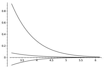
Figure 1. The eigenvalues of the Hessian for $D_{16}^{+}$ (two different eigenvalues, left) and $E_{8}\perp E_{8}$ (three different eigenvalues, right) depending on the parameter $\alpha$.

We introduce the following notation: The value in (15) we denote by $\mu(L,\lambda,\alpha)$. We consider $\alpha=\pi$, then

$$\begin{array}[]{lcrlcr}\mu(D_{16}^{+},8,\pi)&=&-0.06196\ldots&\qquad\mu(E_{8}\perp E_{8},0,\pi)&=&-0.13245\ldots\\ \mu(D_{16}^{+},56,\pi)&=&0.36093\ldots&\qquad\mu(E_{8}\perp E_{8},24,\pi)&=&0.07899\ldots\\ &&&\qquad\mu(E_{8}\perp E_{8},120,\pi)&=&0.92480\ldots\end{array}$$

We show in Section 5.4 how to translate numerical computations into rigorous bounds.

5.3. Dimension 24

The Niemeier lattices are the even unimodular lattices in dimension $24$ which have vectors of squared norm $2$. A classification of Niemeier gave that there are $23$ Niemeier lattices and Venkov realized that they can be characterized by their root system. The theta series of a Niemeier lattice $L$ with root system $L(2)$ is the modular form of weight $12$

$$\Theta_{L}(\tau)=E_{4}^{3}(\tau)+(|L(2)|-720)\Delta(\tau)=1+|L(2)|q+\cdots.$$

The cusp form of weight $16$ is $E_{4}\Delta$. We apply Theorem 3.1 together with Theorem 4.1 and Theorem 4.7 to determine the signature of the Hessian at $\alpha=\pi$. We collect our results in Table 2. For large values of $\alpha$ Corollary 3.2 shows that only the Niemeier lattices with irreducible root systems, namely $A_{24}$ and $D_{24}$, are local minima for $f_{\alpha}$-potential energy. All other Niemeier lattices are saddle points for $f_{\alpha}$-potential energy for $\alpha$ large enough.

$\bm{L(2)}$	$\bm{|L(2)|}$	$\bm{h}$	$\bm{\lambda}$	multiplicity	$\bm{\mu(L,\lambda,\pi)}$
$A_{1}^{24}$	$48$	$2$	$0$	$276$	$0.0018\ldots$
			$8$	$23$	$0.1044\ldots$
$A_{2}^{12}$	$72$	$3$	$0$	$264$	$-0.0050\ldots$
			$6$	$24$	$0.0718\ldots$
			$12$	$11$	$0.1488\ldots$
$A_{3}^{8}$	$96$	$4$	$0$	$252$	$-0.0120\ldots$
			$4$	$16$	$0.0392\ldots$
			$8$	$24$	$0.0905\ldots$
			$16$	$7$	$0.1931\ldots$
$A_{4}^{6}$	$120$	$5$	$0$	$240$	$-0.0189\ldots$
			$4$	$30$	$0.0323\ldots$
			$10$	$24$	$0.1092\ldots$
			$20$	$5$	$0.2375\ldots$
$A_{5}^{4}D_{4}$	$144$	$6$	$0$	$230$	$-0.0259\ldots$
			$4$	$36$	$0.0253\ldots$
			$8$	$9$	$0.0766\ldots$
			$12$	$20$	$0.1279\ldots$
			$24$	$4$	$0.2818\ldots$
$D_{4}^{6}$	$144$	$6$	$0$	$240$	$-0.0259\ldots$
			$8$	$54$	$0.0766\ldots$
			$24$	$5$	$0.2818\ldots$
$A_{6}^{4}$	$168$	$7$	$0$	$216$	$-0.0328\ldots$
			$4$	$56$	$0.0184\ldots$
			$14$	$24$	$0.1466\ldots$
			$28$	$3$	$0.3262\ldots$
$A_{7}^{2}D_{5}^{2}$	$192$	$8$	$0$	$214$	$-0.0398\ldots$
			$4$	$40$	$0.0114\ldots$
			$8$	$20$	$0.0627\ldots$
			$12$	$8$	$0.1140\ldots$
			$16$	$14$	$0.1653\ldots$
			$32$	$3$	$0.3705\ldots$
$A_{8}^{3}$	$216$	$9$	$0$	$192$	$-0.0467\ldots$
			$4$	$81$	$0.0045\ldots$
			$18$	$24$	$0.1840\ldots$
			$36$	$2$	$0.4149\ldots$
$A_{9}^{2}D_{6}$	$240$	$10$	$0$	$189$	$-0.0537\ldots$
			$4$	$70$	$-0.0024\ldots$
			$8$	$15$	$0.0488\ldots$
			$16$	$5$	$0.1514\ldots$
			$20$	$18$	$0.2027\ldots$
			$40$	$2$	$0.4592\ldots$
$D_{6}^{4}$	$240$	$10$	$0$	$216$	$-0.0537\ldots$
			$8$	$60$	$0.0488\ldots$
			$16$	$20$	$0.1514\ldots$
			$40$	$3$	$0.4592\ldots$
$E_{6}^{4}$	$288$	$12$	$0$	$216$	$-0.0676\ldots$
			$12$	$80$	$0.0862\ldots$
			$48$	$3$	$0.5479\ldots$

Table 2. The eigenvalues of the Hessian of the Niemeier lattices for $\alpha=\pi$.

$\bm{L(2)}$	$\bm{|L(2)|}$	$\bm{h}$	$\bm{\lambda}$	multiplicity	$\bm{\mu(L,\lambda,\pi)}$
$A_{11}D_{7}E_{6}$	$288$	$12$	$0$	$185$	$-0.0676\ldots$
			$4$	$54$	$-0.0163\ldots$
			$8$	$21$	$0.0349\ldots$
			$12$	$20$	$0.0862\ldots$
			$20$	$6$	$0.1888\ldots$
			$24$	$11$	$0.2401\ldots$
			$48$	$2$	$0.5479\ldots$
$A_{12}^{2}$	$312$	$13$	$0$	$144$	$-0.0746\ldots$
			$4$	$130$	$-0.0233\ldots$
			$26$	$24$	$0.2588\ldots$
			$52$	$1$	$0.5923\ldots$
$D_{8}^{3}$	$336$	$14$	$0$	$192$	$-0.0815\ldots$
			$8$	$84$	$0.0210\ldots$
			$24$	$21$	$0.2262\ldots$
			$56$	$2$	$0.6366\ldots$
$A_{15}D_{9}$	$384$	$16$	$0$	$135$	$-0.0954\ldots$
			$4$	$104$	$-0.0441\ldots$
			$8$	$36$	$0.0071\ldots$
			$28$	$8$	$0.2636\ldots$
			$32$	$15$	$0.3149\ldots$
			$64$	$1$	$0.7253\ldots$
$A_{17}E_{7}$	$432$	$18$	$0$	$119$	$-0.1093\ldots$
			$4$	$135$	$-0.0580\ldots$
			$16$	$27$	$0.0958\ldots$
			$36$	$17$	$0.3523\ldots$
			$72$	$1$	$0.8140\ldots$
$D_{10}E_{7}^{2}$	$432$	$18$	$0$	$189$	$-0.1093\ldots$
			$8$	$45$	$-0.0067\ldots$
			$16$	$54$	$0.0958\ldots$
			$32$	$9$	$0.3010\ldots$
			$72$	$2$	$0.8140\ldots$
$D_{12}^{2}$	$528$	$22$	$0$	$144$	$-0.1371\ldots$
			$8$	$132$	$-0.0345\ldots$
			$40$	$22$	$0.3758\ldots$
			$88$	$1$	$0.9914\ldots$
$A_{24}$	$600$	$25$	$4$	$275$	$-0.1067\ldots$
			$50$	$24$	$0.4832\ldots$
$D_{16}E_{8}$	$720$	$30$	$0$	$128$	$-0.1928\ldots$
			$8$	$120$	$-0.0902\ldots$
			$24$	$35$	$0.1150\ldots$
			$56$	$15$	$0.5254\ldots$
			$120$	$1$	$1.3462\ldots$
$E_{8}^{3}$	$720$	$30$	$0$	$192$	$-0.1928\ldots$
			$24$	$105$	$0.1150\ldots$
			$120$	$2$	$1.3462\ldots$
$D_{24}$	$1104$	$46$	$8$	$276$	$-0.2014\ldots$
			$88$	$23$	$0.8246\ldots$

Table 2. (continued).

5.4. Dimension 32

In dimension 32 the even unimodular lattice have not been classified yet. Some partial results are known: There are at least 80 million of them, see Serre [20]. King [13] showed that there are at least ten million even unimodular lattices without roots in dimension 32. Kervaire [12] classified all indecomposable even unimodular lattices in dimension $32$ that possess a full root system.

In general an even unimodular lattice need not even be a critical point for the Gaussian potential function. The first such examples can be found in dimension $32$, we briefly discuss one of them.

For example there exists a lattice $L\subseteq\mathbb{R}^{32}$ with complete root system $A_{1}^{8}A_{3}^{8}$, see Kervaire [12]. We split the summation in the gradient into the contribution of the root system and the contribution of all larger shells

$$\begin{split}\langle\nabla\mathcal{E}(f_{\alpha},L),H\rangle&=-\alpha\sum_{x\in L\setminus\{0\}}H[x]e^{-\alpha\|x\|^{2}}\\ &=-\alpha e^{-2\alpha}\left(\sum_{x\in L(2)}H[x]\right)-\alpha\left(\sum_{x\in L\setminus(\{0\}\cup L(2))}H[x]e^{-\alpha\|x\|^{2}}\right).\end{split}$$

We firstly evaluate

$$\sum_{x\in L(2)}H[x]=\langle H,\sum_{x\in L(2)}xx^{\sf T}\rangle$$

and use the fact that $A_{1}$ and $A_{3}$ form spherical $2$-designs and so

$$\sum_{x\in L(2)}xx^{\sf T}=2h(A_{1})I_{8}\oplus 2h(A_{3})I_{24}=4I_{8}\oplus 8I_{24}.$$

The matrix $H=24I_{8}\oplus(-8)I_{24}$ has trace zero and gives

$$\sum_{x\in L(2)}H[x]=24\cdot 4\cdot 8-8\cdot 8\cdot 24=-4\cdot 8\cdot 24=-768\neq 0.$$

Now, by the eigenvalue bounds for $H[x]$ coming from the Rayleigh-Ritz principle, we find that

$$-8=\lambda_{\min}(H)\leq\frac{H[x]}{\|x\|^{2}}\leq\lambda_{\max}(H)=24.$$

This allows to organize summation over all lattice vectors of squared length at least $4$ by shells

$$-8\sum_{m\geq 2}a_{m}\cdot 2m\cdot e^{-\alpha(2m)}\leq\sum_{x\in L\setminus(\{0\}\cup L(2))}H[x]e^{-\alpha\|x\|^{2}}\leq 24\sum_{m\geq 2}a_{m}\cdot 2m\cdot e^{-\alpha(2m)},$$

where $a_{m}=|L(2m)|$ ist the $m$-th coefficient of the theta series $\Theta_{L}$ of $L$.

Combining the above, we see that it suffices to show

(33) $$24\sum_{m\geq 2}a_{m}\cdot 2m\cdot e^{-\alpha(2m)}\leq 768\cdot e^{-2\alpha}.$$

For this we write $\Theta_{L}$ in the form $\Theta_{L}=E_{16}+f$, where $f$ is a cusp form of weight $16$. Let

$$E_{16}(\tau)=\sum_{m=0}^{\infty}b_{m}q^{m}\quad\text{and}\quad f(\tau)=\sum_{m=1}^{\infty}c_{m}q^{m},$$

in particular $b_{m}=-\frac{32}{B_{16}}\sigma_{15}(m)=16320/3617\sigma_{15}(m)$ and so $c_{1}=-16320/3617$. We use the estimate $\sigma_{k-1}(m)\leq\zeta(k-1)m^{k-1}$, where $\zeta$ is the Riemann zeta function, and get $b_{m}\leq 4.6m^{15}$. To bound $c_{m}$ we use (4), the facts $\ell=1$, $d(m)\leq 2\sqrt{m}$, and get $|c_{m}|\leq 1.2\cdot 10^{10}m^{8}$. Together,

(34) $$|a_{m}|\leq 4.6m^{15}+1.2\cdot 10^{10}m^{8}.$$

We evaluate for $\alpha=14$, this gives

$$\sum_{m\geq 2}a_{m}\cdot 2m\cdot e^{-28m}\leq 9.2\sum_{m=2}^{\infty}m^{16}\cdot e^{-28m}+2.4\cdot 10^{10}\sum_{m=2}^{\infty}m^{9}\cdot e^{-28m}.$$

By Lemma 2.2 we have

$$\sum_{m=2}^{\infty}m^{16}e^{-28m}\leq 3.2\cdot 10^{-20}+(28)^{-17}\Gamma(17,56)\leq 3.3\cdot 10^{-20},$$

and

$$\sum_{m=2}^{\infty}m^{9}e^{-28m}\leq 2.5\cdot 10^{-22}+(2\alpha)^{-10}\Gamma(10,56)\leq 2.6\cdot 10^{-22}.$$

Putting everything together for $\alpha=14$ in (33) we find

$$\begin{split}24\sum_{m\geq 2}a_{m}\cdot 2m\cdot e^{-\alpha(2m)}\;\leq\;&24\left(9.2\cdot 3.3\cdot 10^{-20}+2.4\cdot 10^{10}\cdot 2.6\cdot 10^{-22}\right)\\ \leq\;&24\left(3.1\cdot 10^{-19}+6.3\cdot 10^{-12}\right)\\ \leq\;&1.6\cdot 10^{-10}\\ \leq\;&768\cdot e^{-28}.\end{split}$$

This shows that this lattice is not a critical point for the Gaussian potential function $e^{-14r}$.

Last, but not least, we show that all even unimodular lattices without roots in dimension $32$ are local maxima for the Gaussian potential function $e^{-\pi r}$. All the even unimodular lattices in dimension 32 without roots have the same theta series, for such a lattice $L\subseteq\mathbb{R}^{32}$ we have

$$\begin{split}\Theta_{L}(\tau)\;=\;&E_{4}^{4}(\tau)-960E_{4}(\tau)\Delta(\tau)\\ \;=\;&1+146880q^{2}+64757760q^{3}+4844836800q^{4}+137695887360q^{5}\\ &\quad+2121555283200q^{6}+21421110804480q^{7}\\ &\quad+158757684004800q^{8}+\cdots\end{split}$$

All shells of $L$ form spherical 4-designs, so $L$ is critical for all Gaussian potential functions and we can compute the eigenvalue of the Hessian (7) using (12). For $\alpha=\pi$ we compute the first summands of the series and get

$$\frac{1}{n(n+2)}\sum_{m=0}^{8}a_{m}\pi(2m)(\pi(2m)-(n/2+1))e^{-\pi(2m)}<-0.00027.$$

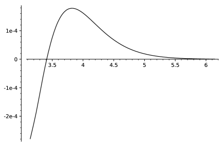
Figure 2. The eigenvalue of the Hessian for even unimodular lattices in dimension $32$ without roots depending on the parameter $\alpha$.

Now we argue that the tail of the series is so small that the entire series is strictly negative.

For this, again, we use the bound (34) for the coefficients $a_{m}$ of $\Theta_{L}$, and we estimate

$$\left|\sum_{m=9}^{\infty}a_{m}\pi(2m)(\pi(2m)-(n/2+1))e^{-\pi(2m)}\right|\leq\sum_{m=9}^{\infty}|a_{m}|(2\pi m)^{2}e^{-2\pi m},$$

and

$$\sum_{m=9}^{\infty}|a_{m}|(2\pi m)^{2}e^{-2\pi m}\leq 181.7\sum_{m=9}^{\infty}m^{17}e^{-2\pi m}+4.8\cdot 10^{11}\sum_{m=9}^{\infty}m^{10}e^{-2\pi m}.$$

Again, by Lemma 2.2

$$\sum_{m=9}^{\infty}m^{17}e^{-2\pi m}\leq 4.7\cdot 10^{-9}+(2\pi)^{-18}\Gamma(18,18\pi)\leq 5.8\cdot 10^{-9}.$$

Similarly,

$$\sum_{m=9}^{\infty}m^{10}e^{-2\pi m}\leq 9.7\cdot 10^{-16}+(2\pi)^{-11}\Gamma(11,18\pi)\leq 1.2\cdot 10^{-15}.$$

Altogether:

$$\begin{split}&\left|\frac{1}{n(n+2)}\sum_{m=9}^{\infty}a_{m}\pi(2m)(\pi(2m)-(n/2+1))e^{-\pi(2m)}\right|\\ &\leq\;1088^{-1}\left(181.7\cdot 5.8\cdot 10^{-9}+4.8\cdot 10^{11}\cdot 1.2\cdot 10^{-15}\right)\\ &\leq\;5.4\cdot 10^{-7}.\end{split}$$

Hence, we showed that for $\alpha=\pi$ the even unimodular lattices in dimension $32$ without roots are local maxima for the Gaussian potential function. This answers a question of Regev and Stephens-Davidowitz [17].

References

- [1] J.-B. Bost, Exposé Bourbaki 1151: Réseaux euclidiens, séries thêta et pentes (d’après W. Banaszczyk, O. Regev, D. Dadush, N. Stephens-Davidowitz, …), Séminaire Bourbaki Octobre 2018 71e année, 2018–2019, no 1152.
- [2] H. Cohn, A. Kumar, S.D. Miller, D. Radchenko, M. Viazovska, Universal optimality of the and Leech lattices and interpolation formulas, Ann. of Math. (2), to appear, arXiv:1902.05438.
- [3] J.H. Conway, N.J.A. Sloane, Sphere packings, lattices, and groups, Springer, 1988.
- [4] R. Coulangeon, Spherical designs and zeta functions of lattices, Int. Math. Res. Not. IMRN (2006), 1–16.
- [5] R. Coulangeon, A. Schürmann, Energy minimization, periodic sets and spherical designs, Int. Math. Res. Not. IMRN (2012), 829–848.
- [6] M. Dutour Sikirić, A. Schürmann, F. Vallentin, Inhomogeneous extreme forms, Ann. Inst. Fourier (Grenoble) 62 (2012), 2227–2255.
- [7] W. Ebeling, Lattices and Codes, Vieweg, 1994.
- [8] W. Fulton, J.W. Harris, Representation Theory: A First Course, Springer, 1991.
- [9] J.S. Frame, The classes and representations of the groups of lines and bitangents, Ann. Mat. Pura Appl. (4) 32 (1951), 83–119.
- [10] J.S. Frame, The characters of the Weyl group , pp. 111–130 in: 1970 Computational Problems in Abstract Algebra (Proc. Conf., Oxford, 1967), Pergamon, 1970.
- [11] P. Jenkins, J. Rouse, Bounds for coefficients of cusp forms and extremal lattices, Bull. Lond. Math. Soc. 43 (2011), 927–938.
- [12] M. Kervaire, Unimodular lattices with a complete root system, Enseign. Math. 40 (1994), 59–140.
- [13] O.D. King, A mass formula for unimodular lattices without roots, Math. Comp. 72 (2002), 839–863.
- [14] L.J. Mordell, The definite quadratic form in eight variables with determinant unity, J. Math. Pures Appl. 17 (1938), 41–46.
- [15] G. Nebe, Boris Venkov’s theory of lattices and spherical designs, pages 1–19 in: Diophantine methods, lattices, and arithmetic theory of quadratic forms, Contemp. Math., 587, Amer. Math. Soc., 2013.
- [16] H.-V. Niemeier, Definite quadratische Formen der Dimension 24 und Diskriminante 1, J. Number Theory 5 (1973), 142–178.
- [17] O. Regev, N. Stephens-Davidowitz, A reverse Minkowski theorem, in: STOC, 2017: Proceedings of the 49th Annual ACM SIGACT Symposium on Theory of Computing, pp 941–953, arXiv:1611.05979 [math.MG].
- [18] The Sage Development Team, SageMath, the Sage Mathematics Software System (Version 9.1), http://www.sagemath.org, 2020.
- [19] P. Sarnak, A. Strömbergsson, Minima of Epstein’s zeta function and heights of flat tori, Invent. Math. 165 (2006), 115–151.
- [20] J.-P. Serre, A Course in Arithmetic, Springer-Verlag, 1973.
- [21] B. Simon, Harmonic Analysis, A Comprehensive Course in Analysis, Part 3, AMS, 2015.
- [22] F.H. Stillinger, Phase transitions in the Gaussian core system, J. Chem. Phys. 65 (1976), 3968–3974.
- [23] B.B. Venkov, The classification of integral even unimodular 24-dimensional quadratic forms, Trudy Math. Inst. Steklov 148 (1978), 65–76 (Proc. Steklov Inst. Math. 148 (1980), 63–74).
- [24] B.B. Venkov, Réseaux et designs sphériques, pages 10–86 in: Réseaux euclidiens, designs sphériques et formes modulaires, Monogr. Enseign. Math., 37, 2001.
- [25] D.V. Widder, The Laplace Transform, Princeton University Press, 1941.
- [26] E. Witt, Eine Identität zwischen Modulformen zweiten Grades, Abh. Math. Semin. Univ. Hambg. 14 (1941) 323–337.