Investigating global convective dynamos with mean-field models:
full spectrum of turbulent effects required

Abstract

The role of turbulent effects for dynamos in the Sun and stars continues to be debated. Mean-field (MF) theory provides a broadly used framework to connect these effects to fundamental magnetohydrodynamics. While inaccessible observationally, turbulent effects can be directly studied using global convective dynamo (GCD) simulations. We measure the turbulent effects in terms of turbulent transport coefficients, based on the MF framework, from an exemplary GCD simulation using the test-field method. These coefficients are then used as an input into an MF model. We find a good agreement between the MF and GCD solutions, which validates our theoretical approach. This agreement requires all turbulent effects to be included, even those which have been regarded as unimportant so far. Our results suggest that simple dynamo models, as are commonly used in the solar and stellar community, relying on very few, precisely fine-tuned turbulent effects, may not be representative of the full dynamics of dynamos in global convective simulations and astronomical objects.

1 Introduction

The magnetic fields of the Sun and other cool stars are generated by a dynamo mechanism operating in their interiors. Despite plentiful observations, over an extensive history with many at high resolution, the nature of the solar dynamo is not yet fully understood. One of the difficulties lies in the poor knowledge of the turbulent effects, which are expected to play an important part in the magnetic field generation. These effects are often described by a parameterization based on mean-field (MF) theory. Because of their intricacy, however, it is common in the solar context to simplify the parameterizations such that they can be fine-tuned to fit some of the magnetic field observations (e.g. Karak et al., 2014; Cameron & Schüssler, 2015). As an alternative approach, global convective dynamo (GCD) models can be used to self-consistently generate these turbulent effects. While these models have parameters far from real astrophysical objects, they currently represent the best laboratories to this end. Nevertheless, investigating the nature of dynamos in GCD is very challenging and needs an analysis tool, which connects properties of the GCD to established dynamo theories. In the recent years the test-field method (TFM) has become such a well-established tool to measure the turbulent transport coefficients (TTCs), quantifying the turbulent effects, in such GCD models (Schrinner et al., 2005, 2007, 2011, 2012; Schrinner, 2011; Warnecke, 2018; Warnecke et al., 2018; Viviani et al., 2019; Warnecke & Käpylä, 2020). Already in these studies, it was found that the turbulent effects play an important part in the magnetic field evolution. However, to show that the TTCs measured by the TFM capture the most important details of the magnetic field evolution, the coefficients need to be employed in an MF model and the results to be compared with the GCD simulations. Furthermore, only with the use of an MF model one will be able to pinpoint which of these turbulent effects are essential for a full understanding of dynamo action in the GCD. Steps in this direction, beyond the works of Schrinner et al., have been performed using a small subset of TTCs ($\alpha$ tensor and turbulent pumping) obtained from a GCD simulation using the singular value decomposition (SVD) method (Simard et al., 2013; Simard & Charbonneau, 2020).

In our work, we use in an MF model the TTCs of an exemplary GCD model, the magnetic field evolution of which shows similarities to the Sun, to investigate whether or not this evolution can be reproduced. Furthermore, we will investigate which minimal subset of the coefficients is essential to reproduce the dynamo solution and hence determine whether or not it can be described by any of the commonly employed simple dynamo models. We will conclude by discussing the further implications of the results.

2 Models and Methods

We analyze Run M5 of Warnecke (2018) and Warnecke & Käpylä (2020), a GCD simulation in a spherical shell. It has a rotation rate roughly four times higher than the Sun, in terms of the Coriolis number and a Rayleigh number two orders of magnitude larger than the critical one for the onset of convection (Warnecke et al., 2018); see also Käpylä et al. (2013) and Warnecke (2018) for more details on this run and its comparison with solar parameters. The axisymmetric (azimuthally averaged) part of the generated magnetic field shows rather regular oscillations with a magnetic cycle period $P_{\rm cyc}=P_{\rm cyc}^{\rm{GCD}}\equiv 4.4\pm 0.6$ yr (Warnecke, 2018), and exhibits both equatorward and poleward branches of field migration in the butterfly (time–latitude) diagram, thus capturing main solar cycle features; see Figure 1. We note here that this is not a one-to-one representation of the Sun and its dynamo, but a good example of state-of-the-art models of solar-like stars in the scientific community (e.g. Augustson et al., 2015; Strugarek et al., 2017). A second, weaker dynamo mode with a much shorter period of about $0.11$ yr is present at low latitudes near the surface; see Figure 1 and Käpylä et al. (2016) for a detailed discussion.

Our MF approach employs azimuthal averaging, indicated by an overbar, which adheres to the Reynolds rules; fluctuating fields are indicated by primes. The MF induction equation reads

$$\partial_{t}\overline{\mbox{\boldmath$B$}}{}=\mbox{\boldmath$\nabla$}{}\times\left(\overline{\bm{U}}\times\overline{\mbox{\boldmath$B$}}{}+\mbox{\boldmath${\cal E}$}{}\right)-\mbox{\boldmath$\nabla$}{}\times\eta\mbox{\boldmath$\nabla$}{}\times\overline{\mbox{\boldmath$B$}}{},$$ (1)

where $\overline{\bm{U}}$ and $\overline{\mbox{\boldmath$B$}}{}$ are mean flow and mean magnetic field, respectively, and $\eta$ is the magnetic diffusivity. To establish the MF model, a parameterization of the mean electromotive force $\mbox{\boldmath${\cal E}$}{}=\overline{\mbox{\boldmath$u^{\prime}$}{}\times\mbox{\boldmath$B^{\prime}$}{}}$ in terms of the mean field itself is crucial. Employing Taylor expansion, leaving out time derivatives and restricting to first-order spatial derivatives, a commonly quoted ansatz reads (Krause & Rädler, 1980)

$$\mbox{\boldmath${\cal E}$}{}=\mbox{\boldmath$\alpha$}{}\cdot\overline{\mbox{\boldmath$B$}}{}+\mbox{\boldmath$\gamma$}{}\times\overline{\mbox{\boldmath$B$}}{}-\mbox{\boldmath$\beta$}{}\cdot\left(\mbox{\boldmath$\nabla$}{}\times\overline{\mbox{\boldmath$B$}}{}\right)-\mbox{\boldmath$\delta$}{}\times\left(\mbox{\boldmath$\nabla$}{}\times\overline{\mbox{\boldmath$B$}}{}\right)-\mbox{\boldmath$\kappa$}{}\cdot\left(\mbox{\boldmath$\nabla$}{}\overline{\mbox{\boldmath$B$}}{}\right)^{(s)},$$ (2)

where $(\mbox{\boldmath$\nabla$}{}\overline{\mbox{\boldmath$B$}}{})^{(s)}$ is the symmetric part of the (covariant) derivative tensor of $\overline{\mbox{\boldmath$B$}}{}$. The most general representation of ${\cal E}$ at some position $(r,\theta)$ and time $t$ would involve a convolution integral over a neighborhood of $(r,\theta,t)$, thus covering nonlocal and memory effects (Krause & Rädler, 1980). In contrast, Eq. (2) is completely instantaneous in time and only rudimentarily nonlocal in space.

Figure 1: Time–latitude (butterfly) diagrams of mean radial, $\overline{B}_{r}$, and azimuthal, $\overline{B}_{\phi}$, magnetic field from GCD (top) and the MF model (bottom) at fractional radius 0.95. The rightmost panels show a zoom-in to the first five years of the middle panels. The TTCs are symmetrized, and $\alpha$ is scaled by 1.5, while exponential growth has been compensated for clarity. The color range is cut to make the northern hemisphere more visible. Black lines: zero contours of $\overline{B}_{\phi}$ from the MF model at the same time. See Appendix A for butterfly diagrams of the corresponding pure-parity solutions.

$\alpha$ and $\beta$ are symmetric rank-two tensors, $\gamma$ and $\delta$ are vectors, and $\kappa$ is a rank-three tensor, with symmetry $\kappa_{ijk}=\kappa_{ikj}$. These five tensors can be associated with different turbulent effects important for the magnetic field evolution: the $\alpha$ effect (Steenbeck et al., 1966) can lead to field amplification via helical flows, e.g. in stratified rotating convection, the $\gamma$ effect describes turbulent pumping of the mean magnetic field, in analogy to a mean flow. $\beta$ describes turbulent diffusion; and the $\delta$, or Rädler effect (Rädler, 1969), can lead to dynamo action in the presence of, e.g., $\alpha$ effect or shear, but not alone (Brandenburg & Subramanian, 2005). The physical interpretation of $\kappa$ is yet unclear, but quite generally it may contribute to both amplification and diffusion of $\overline{\mbox{\boldmath$B$}}{}$. More details on these effects and its parameterization can be found, e.g., in Krause & Rädler (1980) and Brandenburg & Subramanian (2005).

Accounting for all symmetries in Eq. (2) and $\partial_{\phi}\overline{B}_{r,\theta,\phi}=0$, a total of 27 coefficients must be identified to close Eq. (1). Note that due to the axisymmetry of $\overline{\mbox{\boldmath$B$}}{}$, the representation of Eq. (2) is nonunique. In particular, components of $\kappa$ can be recast into components of $\beta$. Here we have chosen a formulation of $\beta$ and $\kappa$ that maximizes the number of vanishing entries in $\kappa$, that is, allocates as much information on the diffusive aspects of turbulent transport as possible in $\beta$, thus facilitating physical interpretation; see Viviani et al. (2019) for details.

To determine the required 27 coefficients we apply the quasi-kinematic TFM to the original GCD model. The original TTCs are already published (Warnecke, 2018; Warnecke & Käpylä, 2020) and available online. The TFM, as utilized in Schrinner et al. (2005, 2007) and Warnecke et al. (2018), requires nine additional realizations of the induction equation for the fluctuating magnetic field $B^{\prime}$ to be solved simultaneously with the GCD simulation. They are obtained by replacing $\overline{\mbox{\boldmath$B$}}{}$ in $\mbox{\boldmath$\nabla$}{}\times\big{(}\mbox{\boldmath$u^{\prime}$}{}\times\overline{\mbox{\boldmath$B$}}{}\big{)}$ by one out of nine linearly independent test fields $\overline{\mbox{\boldmath$B$}}{}^{(i)}$, $i=1,\ldots,9$, while the velocity $\mbox{\boldmath$u$}{}=\overline{\bm{U}}+\mbox{\boldmath$u^{\prime}$}{}$ is taken directly from the GCD simulation (see Schrinner et al., 2007, for details). Employing the corresponding electromotive forces $\mbox{\boldmath${\cal E}$}{}^{(i)}=\overline{\mbox{\boldmath$u^{\prime}$}{}\times\mbox{\boldmath$B^{\prime}$}{}^{(i)}}$, a uniquely solvable linear equation system for the coefficients in Eq. (2) can be formed.

In the stationary, saturated state of the GCD simulation the magnetic field acquires dynamically significant strength. Hence, the velocity and TTCs derived from it are already magnetically quenched, that is, they differ from their counterparts in the nonmagnetic (or kinematic) state. Consequently, the MF model of Eq. (1) is, strictly speaking, valid only for the mean field that is observed in the GCD simulation (Brandenburg et al., 2010).

We subject the TTCs to the following preprocessing steps: firstly, we exclude the noise arising from large variations at small time scales (Warnecke et al., 2018) by averaging over their full time series; secondly, to damp spatial fluctuations, we apply a Gaussian smoothing in $\theta$ using a kernel with a standard deviation equal to the grid spacing; thirdly, we remove negative values from the diagonal $\beta$ components and apply a lower threshold of $-0.7\eta$ for $\kappa_{\phi r\theta}$ to avoid unphysical local instabilities. For consistency, $\overline{\bm{U}}$ is time averaged, too. Additionally, we reduce the original resolution of the coefficients from $180\times 256$ (radial $\times$ latitudinal) to $40\times 64$ for computational efficiency.

The set of equations for GCD admits solutions with “pure” equatorial symmetries, that is, equatorially symmetric velocity, density, and entropy fields, combined with an either symmetric (S) or antisymmetric (A) magnetic field. The degree of equatorial symmetry of a field is quantified by the parity $P$, which takes values between $-1$ for A and $+1$ for S. In the GCD simulation, the parity of the magnetic field continuously varies between $+1$ and $-1$, indicating that A and S dynamo modes of similar strength are competing for dominance (Käpylä et al., 2016); see also Appendix A. Each of the measured TTC components, however, has near pure parity of one or the other (Warnecke et al., 2018). Therefore, to study the competing pure modes in isolation in the MF model we employ TTCs, properly symmetrized so as to restrict their parity to, respectively, $P=\pm 1$.

For the MF simulations we solve Eq. (1) using the preprocessed $\overline{\bm{U}}$ and TTCs and the same $\eta$ as in the GCD model without employing any quenching terms. Hence, the MF model is entirely linear, and by virtue of the temporal constancy of all its coefficients, all solutions show exponential behavior, in general with a complex increment. The mean magnetic field is initialized by a weak random seed.

All simulations were performed using the Pencil Code (Pencil Code Collaboration et al., 2021); see Tuomisto (2019) for details of its MF module.

3 Results

First we look at an MF solution, the parity of which is not restricted while the symmetrized TTCs are employed, and compare with the one of the GCD model. If the $\alpha$ tensor is scaled by a factor $f_{\alpha}$ between $1.40$ and $1.525$ we find growing oscillatory solutions, which resemble the GCD solution very well, as shown in Figure 1. Their periods of $4.5$–$4.9$ yr are in close agreement with $P_{\rm cyc}^{\rm{GCD}}\equiv 4.4\pm 0.6$ yr (Warnecke, 2018). The butterfly diagram is well reproduced, too: the poleward migrating $\overline{B}_{r}$ pattern has the same shape and slope as in the GCD simulation. In $\overline{B}_{\phi}$, the agreement of the pattern shapes is also striking as signified by the zero contours of the MF solution plotted over the GCD one. Deviations are visible at the highest latitudes where the test-field measurements are likely to be contaminated by the unphysical latitudinal boundaries. Also, at midlatitudes patches of equal polarity appear not to be equatorwards connected as in the GCD solution.

Like the GCD solution, this MF one is neither purely antisymmetric nor symmetric about the equator. See Appendix A for details of the corresponding pure-parity solutions of the MF model. The zoom-in to the early phases of the MF model (see the lower rightmost panel of Figure 1) shows the high-frequency, poleward migrating mode with roughly $0.11$ yr period length at low latitudes. Field migration and period of this mode match closely those of the GCD. While it is regular in the MF model, it appears temporally incoherent in GCD, agreeing with the findings of Käpylä et al. (2016) for a very similar run. Given the absence of nonlinearities, this mode becomes subdominant in the MF model. We note here that the absence of nonlinearities also implies that there is no interaction between the two pure-parity modes of the MF model.

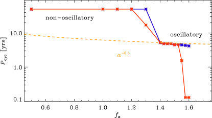
Figure 2: Cycle period $P_{\rm cyc}$ as function of the scaling factor $f_{\alpha}$. Red: S, blue: A solutions. Nonoscillatory solutions have been assigned $P_{\rm cyc}=50$ yr. Dashed line: scaling of $P_{\rm cyc}\sim\alpha^{-0.5}$ according to a Parker dynamo wave.

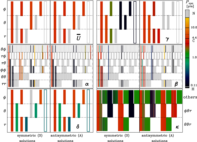
Figure 3: S and A solutions for all combinations of turned-on components for each coefficient tensor with $P_{\rm cyc}$ coded by colors. Gray: nonoscillatory (N), red: correct oscillatory (C), and dark blue: high-frequency oscillatory (H) solutions. For $\kappa$, “others” includes all coefficients other than $\kappa_{\phi\theta r}$ and $\kappa_{\theta\theta r}$. Empty boxes or dashed vertical lines: all components are turned off (not shown for $\kappa$). Dotted lines in color bar: interval (3.0 … 6.0) yr.

We have repeated some of the MF runs with the nonsymmetrized TTCs. Their slight hemispheric asymmetries are sufficient to excite a strongly asymmetric eigenmode, such that one hemisphere exhibits a magnetic field up to two orders of magnitude stronger than the other. The GCD simulation does not show such strong disparities, which we attribute to the nonlinearities in the GCD providing a self-regulation mechanism: whenever significant disparity occurs, the hemisphere showing the higher dynamo efficiency would also experience a stronger back-reaction of the magnetic field on the flow (quenching). Thus, dominance of one hemisphere likely cannot persist for long. Instead, both the TTCs and the mean field will stay close to a state of nearly pure parity. The MF model, being linear, cannot provide such self-regulation. Applying symmetrized coefficients, however, is sufficient to maintain consistent growth between the hemispheres.

The consistencies between the MF and GCD solutions prove that in our case ${\cal E}$, i.e. the contributing turbulent effects, are well described by the parameterization of Eq. (2), meaning that higher-order terms, and also scale dependence and memory effect, can be neglected. Another surprising aspect is that employing only the time-averaged, smoothed, and downsampled TTCs, that is, ignoring their large temporal and small-scale spatial variations, is not detrimental to the agreement with the GCD solution, but might explain the necessity of a moderate upscaling of $\alpha$.

For values of $f_{\alpha}<1.40$, the solutions are growing with a dominantly nonoscillatory field, see Figure 2. Interestingly, the oscillation period is closest to that of the GCD model, when the growth rates of the A and S solutions are nearly identical, hence enabling a mixed solution. For $f_{\alpha}>1.525$, the oscillation period of the S mode is strongly reduced, closely matching that of the high-frequency mode reported for the GCD model. Oscillation periods close to $P_{\rm cyc}^{\rm{GCD}}$ depend only weakly on $f_{\alpha}$, consistent with the expected scaling of the period of an $\alpha\Omega$ dynamo wave, $P_{\rm cyc}\sim\alpha^{-0.5}$ (Parker, 1955; Yoshimura, 1975); see Figure 2. This agrees with earlier findings that direction and period of dynamo waves in GCD models of this kind can be well explained by the Parker–Yoshimura rule (Warnecke et al., 2014, 2018; Warnecke, 2018).

Next we analyze which of the TTCs and mean flow components are essential for reproducing the GCD solution. For this we perform around 2000 MF simulations with $f_{\alpha}=1.5$, where we turn on/off the various components of a certain TTC tensor at a time, while fixing all the others at their nominal values, to investigate the changes in the resulting MF solution. To classify the solutions, we define three different classes based on their period; see Figure 3. The first class (C for “correct”) has a period in the interval (3.0 … 6.0) yr around $P_{\rm cyc}^{\rm{GCD}}$, the second (N) has dominantly nonoscillatory solutions, the third (H for “high frequency”) has oscillatory solutions, close to the near-surface high-frequency dynamo mode with $P_{\rm cyc}=0.11$ yr. For a set of coefficients to be considered essential to reproduce the GCD solution we require that both the S and A solutions fall into class C (details in Table 1 of Appendix C).

First, we consider the effect of $\overline{\bm{U}}$. As illustrated in Figure 3, only solutions with a nonzero $\overline{U}_{\phi}$ are oscillatory with a period close to $P_{\rm cyc}^{\rm{GCD}}$; all other cases have only nonoscillatory solutions. This means that the meridional circulation ($\overline{U}_{r}$,$\overline{U}_{\theta}$) has a negligible contribution, while differential rotation ($\Omega$ effect) is crucial, in clear contrast to the often invoked flux-transport dynamo models (e.g., Karak et al., 2014), where the meridional circulation plays an essential part. All solutions with the full $\alpha$ tensor (or at best missing $\alpha_{\theta\phi}$) fall into class C. Most of the other solutions fall either in the N or H class; see Figure 3. Given the prime importance of $\alpha$ and $\overline{U}_{\phi}$, we conclude that an $\alpha^{2}\Omega$-type dynamo is operating in our model. This is in agreement with the analysis performed in Warnecke & Käpylä (2020) for this run, where the $\alpha$ and $\Omega$ effects were estimated to be comparable in generating the toroidal field; see their Fig. 13. We further point out that the high-frequency mode (class H) is already present if from all the TTCs only certain $\alpha$ components are active, and therefore we identify it as an $\alpha^{2}$ dynamo mode in agreement with earlier findings (Warnecke et al., 2018).

Next, focussing on $\gamma$ and $\delta$, we find that for obtaining class-C solutions, $\gamma_{r}$ and $\gamma_{\theta}$ are important as without one of them only class-N or class-H solutions (additionally one with $P_{\rm cyc}\simeq 1.8$ yr) arise. Likewise, class-C solutions require $\delta_{r}$ and $\delta_{\phi}$; otherwise, only class-N solutions, or periods between classes C and H, are possible; see Figure 3.

The plentiful spectrum of solutions obtained by varying the selection of $\beta$ components (Figure 3) includes a large fraction that is nonphysically unstable. This is because arbitrarily dropping components of $\beta$ can in general destroy its positive definiteness. Interestingly, only when at least the diagonal components plus $\beta_{r\phi}$ and $\beta_{\theta\phi}$ are active, a class-C solution can be reproduced. However, $P_{\rm cyc}=P_{\rm cyc}^{\rm{GCD}}$ requires the full $\beta$ tensor.

From approximately 1500 solutions with various selections of $\kappa$ components, we find that around a third fall into class C, requiring the components $\kappa_{\theta\theta r}$ and $\kappa_{\phi\theta r}$ to be turned on; see Figure 3. Other solutions populate the H class or show periods of $P_{\rm cyc}\simeq 1.7$ yr. Interestingly, many solutions have growth rates larger than that of the full MF model. Thus the $\kappa$ tensor provides additional diffusion to the system. Despite the fact that $\kappa$ is often discarded, we thus find that at least two components are essential for reproducing the GCD solution.

To conclude, we find that a minimum set of TTCs, capable of reproducing the GCD solution, requires $\overline{U}_{\phi}\,(\Omega)$, the full $\alpha$ (except $\alpha_{\theta\phi}$) and $\beta$ tensors, $\gamma_{r}$ and $\gamma_{\theta}$, $\delta_{r}$ and $\delta_{\phi}$, and $\kappa_{\theta\theta r}$ and $\kappa_{\phi\theta r}$. For further testing this, we performed an MF run with the minimal set of coefficients and found a very good match with the GCD simulation; see Table 1 and Appendix B.

4 Conclusion

In our work, we find that the full spectrum of turbulent effects ($\Omega$, $\alpha$, $\beta$, $\gamma_{r}$, $\gamma_{\theta}$, $\delta_{r}$, $\delta_{\phi}$, $\kappa_{\theta\theta r}$, $\kappa_{\phi\theta r}$) is required to reproduce the GCD solution. This has two noteworthy implications.

First, all our findings agree with previous works (Warnecke et al., 2014, 2018; Warnecke, 2018; Warnecke & Käpylä, 2020) insofar as we found that the oscillation period is mostly controlled by the $\alpha$ and $\Omega$ effects and not by the advection due to meridional circulation. This is in stark contrast to simplified flux-transport dynamo models (e.g. Karak et al., 2014), which are commonly invoked to describe the solar dynamo and rely crucially on meridional flow. Furthermore, our results support the concepts of turbulent pumping ($\gamma$) and Rädler effect ($\delta$) to be essential for the dynamo (e.g. Schrinner et al., 2005, 2012; Squire & Bhattacharjee, 2015; Shi et al., 2016; Gent et al., 2017; Warnecke et al., 2018; Viviani et al., 2019; Gressel & Elstner, 2020; Warnecke & Käpylä, 2020; Pipin, 2021).

Second, and more importantly, our work shows that most probably, all turbulent effects considered here are required in the generation of the magnetic field, and therefore are all needed to understand the dynamo operating in GCD simulations (in agreement with Schrinner et al., 2005). Our results hence suggest that simple models based on a handful of fine-tuned coefficients, as commonly used in the solar and stellar context, miss crucial effects at play in GCD models.

Our results are in agreement with the study of Simard et al. (2013), where the authors found that the contributions of the full $\alpha$ and $\gamma$ are important to reproduce their GCD solution. However, they did not consider the effect of $\beta$, $\delta$ and $\kappa$. In addition, their TTCs have been measured using the SVD method, which has been shown to give misleading results if applied to our GCD simulations (Warnecke et al., 2018).

Given the severely limited observability of stellar interiors, even yet in the case of the Sun, such models are currently the only laboratories for quantifying the turbulent effects. Furthermore, simply investigating the electromotive force (e.g. Augustson et al., 2015; Strugarek et al., 2017) or measuring the TTCs and evaluating the relative strengths of the corresponding effects is insufficient. Only by examining these coefficients within an MF model, one can comprehend the dynamo at work in the GCD. Even though the GCD simulations do not attain realistic parameters yet, the understanding of their dynamos is a fundamental step (together with observations and experiments) toward understanding dynamos in many astrophysical objects, in particular in the Sun and other stars.

Appendix A Time–Latitude Diagram of Pure A and S Solutions

We show in Figure 4 the purely symmetric (S) and antisymmetric (A) solutions of the MF model together with the GCD simulation. The solution shown in Figure 1 should be regarded as a weighted sum of these two solutions. As the MF model is linear, the weight depends on the initial condition, and is, in this sense, arbitrary. In that particular MF run, the parity, computed over all depths, is $-0.6$, indicating a larger contribution from the A than the S solution. This also closely matches the GCD simulation, where the parity switches back and forth between $-1$ and $+1$ with a period of around 20 yr; the average parity is $-0.31\pm 0.3$ (see also Käpylä et al., 2016, for a detailed analysis of the parity for a similar GCD simulation). We note that, while the dominating modes of the A and S solutions have equal growth rates, the high-frequency mode has a clearly higher growth rate in the S than in the A solution.

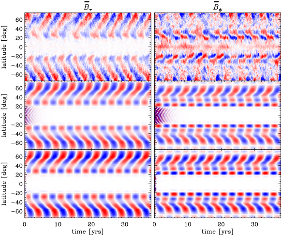
Figure 4: Time–latitude (butterfly) diagrams of mean radial, $\overline{B}_{r}$, and azimuthal, $\overline{B}_{\phi}$, magnetic field from the GCD (top) together with the symmetric (S) and antisymmetric (A) solutions of the MF model (middle and bottom) at fractional radius 0.95 (similar to Figure 1). The TTCs are symmetrized, and $\alpha$ is scaled by 1.5, while exponential growth has been compensated for clarity.

Appendix B Time–latitude diagram for minimal set of coefficients

To show that the minimal set of coefficients, $U_{\phi}$, $\alpha$, $\gamma_{r,\theta}$, $\beta$, $\delta_{r,\phi}$, $\kappa_{\theta\theta r,\phi\theta r}$, is able to reproduce the main features of and the dynamo mode of the GCD simulation, we show in Figure 5 for comparison time–latitude diagrams of the GCD simulation and the MF model. Similar to the MF model including all coefficients, we find a very good agreement, most pronounced at midlatitudes.

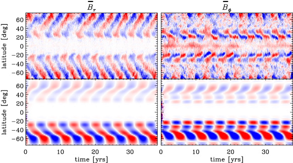
Figure 5: Time–latitude (butterfly) diagrams of mean radial, $\overline{B}_{r}$, and azimuthal, $\overline{B}_{\phi}$, magnetic field from the GCD simulation (top) and the MF model (bottom) at fractional radius 0.95 for the minimal set of coefficients (cf. Figure 1). The TTCs are symmetrized, and $\alpha$ is scaled by 1.5, while exponential growth has been compensated for clarity. The color range is cut to make the northern hemisphere more visible.

Appendix C Solutions close to cycle period of GCD simulation

In Table 1 we show growth rates and oscillation frequencies of those solutions that are close in cycle period to the GCD simulation with $P_{\rm cyc}^{\rm{GCD}}=4.4\pm 0.6$ yr (Class C). The solutions are labeled by their TTC selection. We also define a quality factor $Q$ based on the cycle period defined as

$$Q=1-\left({P_{\rm cyc}-P_{\rm cyc}^{\rm{GCD}}}\over P_{\rm cyc}^{\rm{GCD}}\right)^{2},$$ (C1)

where the exact match of $P_{\rm cyc}$ and $P_{\rm cyc}^{\rm{GCD}}$ yields unity. If the growth rate is negative (no dynamo) we set $Q$ to 0.

Table 1: Solutions with cycles between 3 and 5.8 yr, corresponding to $Q\geq 0.9$. Symmetry indicates symmetric (S) and antisymmetric (A) solutions. $\lambda$ is the growth rate of the volume-integrated rms $\overline{\mbox{\boldmath$B$}}{}$, $P_{\rm cyc}$ is the period of the dominant oscillatory mode and $Q$ is the quality factor defined in Eq. (C1). For each set of TTC selections (separated by solid horizontal lines) all other tensors are fully active. In the penultimate block all active TTCs are listed explicitly for the minimal set of coefficients while the last line shows the solution parameters of the GCD simulation.

TTC Selection Symmetry $\lambda$ (1/yr) $P_{\rm cyc}$ (yr) $Q$ $\overline{U}_{\phi}$ S/A 0.85 4.86 0.99 $\overline{U}_{\theta}$ $\overline{U}_{\phi}$ S/A 0.99 5.28 0.96 $\overline{U}_{r}$ $\overline{U}_{\phi}$ S/A 0.82 4.29 1.00 $\overline{U}_{r}$ $\overline{U}_{\theta}$ $\overline{U}_{\phi}$ S/A 0.92 4.54 1.00 $\alpha_{rr}$ $\alpha_{r\theta}$ $\alpha_{r\phi}$ $\alpha_{\theta\theta}$ $\alpha_{\phi\phi}$ S 1.29 4.67 1.00 A 1.29 4.60 1.00 110mm.5pt.7pt 2pt $\alpha_{rr}$ $\alpha_{r\theta}$ $\alpha_{r\phi}$ $\alpha_{\theta\theta}$ $\alpha_{\theta\phi}$ $\alpha_{\phi\phi}$ S/A 0.92 4.54 1.00 $\alpha_{r\theta}$ $\alpha_{r\phi}$ $\alpha_{\theta\theta}$ $\alpha_{\phi\phi}$ S -0.12 5.69 0.00 $\gamma_{r}$ $\gamma_{\theta}$ S 1.16 5.55 0.93 A 1.15 5.54 0.93 110mm.5pt.7pt 2pt $\gamma_{r}$ $\gamma_{\theta}$ $\gamma_{\phi}$ S/A 0.92 4.54 1.00 $\gamma_{r}$ A 1.30 3.25 0.93 $\beta_{rr}$ $\beta_{r\phi}$ $\beta_{\theta\theta}$ $\beta_{\theta\phi}$ $\beta_{\phi\phi}$ S 0.56 4.00 0.99 A 1.13 4.01 0.99 110mm.5pt.7pt 2pt $\beta_{rr}$ $\beta_{r\theta}$ $\beta_{r\phi}$ $\beta_{\theta\theta}$ $\beta_{\theta\phi}$ $\beta_{\phi\phi}$ S/A 0.92 4.54 1.00 $\beta_{rr}$ $\beta_{\theta\theta}$ $\beta_{\phi\phi}$ S 0.34 4.00 0.99 $\beta_{rr}$ $\beta_{r\phi}$ $\beta_{\theta\theta}$ $\beta_{\phi\phi}$ S 0.37 3.78 0.98 $\beta_{rr}$ $\beta_{r\theta}$ $\beta_{r\phi}$ $\beta_{\theta\theta}$ $\beta_{\phi\phi}$ S 0.16 4.89 0.99 $\delta_{r}$ $\delta_{\phi}$ S/A 0.94 4.86 0.99 $\delta_{r}$ $\delta_{\theta}$ $\delta_{\phi}$ S/A 0.92 4.54 1.00 $\delta_{\theta}$ $\delta_{\phi}$ A 0.50 5.31 0.96 $\overline{U}_{\phi}$ $\alpha$ $\gamma_{r}$ $\gamma_{\theta}$ $\beta$ $\delta_{r}$ $\delta_{\phi}$ $\kappa_{\theta\theta r}$ $\kappa_{\phi\theta r}$ S 1.38 5.58 0.93 A 1.38 5.56 0.93 GCD mixed 0.00 4.4$\pm$0.6 1 to 0.98

References

- Augustson et al. (2015) Augustson, K., Brun, A. S., Miesch, M., & Toomre, J. 2015, ApJ, 809, 149, doi: 10.1088/0004-637X/809/2/149
- Brandenburg et al. (2010) Brandenburg, A., Chatterjee, P., Del Sordo, F., et al. 2010, Phys. Scr, 142, 014028, doi: 10.1088/0031-8949/2010/T142/014028
- Brandenburg & Subramanian (2005) Brandenburg, A., & Subramanian, K. 2005, Phys. Rep., 417, 1, doi: 10.1016/j.physrep.2005.06.005
- Cameron & Schüssler (2015) Cameron, R., & Schüssler, M. 2015, Science, 347, 1333, doi: 10.1126/science.1261470
- Gent et al. (2017) Gent, F. A., Käpylä, M. J., & Warnecke, J. 2017, Astronomische Nachrichten, 338, 885, doi: 10.1002/asna.201713406
- Gressel & Elstner (2020) Gressel, O., & Elstner, D. 2020, MNRAS, 494, 1180, doi: 10.1093/mnras/staa663
- Käpylä et al. (2016) Käpylä, M. J., Käpylä, P. J., Olspert, N., et al. 2016, A&A, 589, A56, doi: 10.1051/0004-6361/201527002
- Käpylä et al. (2013) Käpylä, P. J., Mantere, M. J., Cole, E., Warnecke, J., & Brandenburg, A. 2013, ApJ, 778, 41, doi: 10.1088/0004-637X/778/1/41
- Karak et al. (2014) Karak, B. B., Jiang, J., Miesch, M. S., Charbonneau, P., & Choudhuri, A. R. 2014, Space Sci. Rev., 186, 561, doi: 10.1007/s11214-014-0099-6
- Krause & Rädler (1980) Krause, F., & Rädler, K.-H. 1980, Mean-field Magnetohydrodynamics and Dynamo Theory (Oxford: Pergamon Press)
- Parker (1955) Parker, E. N. 1955, ApJ, 122, 293, doi: 10.1086/146087
- Pencil Code Collaboration et al. (2021) Pencil Code Collaboration, Brandenburg, A., Johansen, A., et al. 2021, JOSS, 6, 2807, doi: 10.21105/joss.02807
- Pipin (2021) Pipin, V. V. 2021, MNRAS, 502, 2565, doi: 10.1093/mnras/stab033
- Rädler (1969) Rädler, K.-H. 1969, Veröffentl. Geod. Geophys, 13, 131
- Saar & Brandenburg (1999) Saar, S. H., & Brandenburg, A. 1999, ApJ, 524, 295, doi: 10.1086/307794
- Schrinner (2011) Schrinner, M. 2011, A&A, 533, A108, doi: 10.1051/0004-6361/201116642
- Schrinner et al. (2011) Schrinner, M., Petitdemange, L., & Dormy, E. 2011, A&A, 530, A140, doi: 10.1051/0004-6361/201016372
- Schrinner et al. (2012) —. 2012, ApJ, 752, 121, doi: 10.1088/0004-637X/752/2/121
- Schrinner et al. (2005) Schrinner, M., Rädler, K.-H., Schmitt, D., Rheinhardt, M., & Christensen, U. 2005, AN, 326, 245, doi: 10.1002/asna.200410384
- Schrinner et al. (2007) Schrinner, M., Rädler, K.-H., Schmitt, D., Rheinhardt, M., & Christensen, U. R. 2007, GApFD, 101, 81, doi: 10.1080/03091920701345707
- Shi et al. (2016) Shi, J.-M., Stone, J. M., & Huang, C. X. 2016, MNRAS, 456, 2273, doi: 10.1093/mnras/stv2815
- Simard & Charbonneau (2020) Simard, C., & Charbonneau, P. 2020, Journal of Space Weather and Space Climate, 10, 9, doi: 10.1051/swsc/2020006
- Simard et al. (2013) Simard, C., Charbonneau, P., & Bouchat, A. 2013, ApJ, 768, 16, doi: 10.1088/0004-637X/768/1/16
- Squire & Bhattacharjee (2015) Squire, J., & Bhattacharjee, A. 2015, ApJ, 813, 52, doi: 10.1088/0004-637X/813/1/52
- Steenbeck et al. (1966) Steenbeck, M., Krause, F., & Rädler, K.-H. 1966, Zeitschrift Naturforschung Teil A, 21, 369
- Strugarek et al. (2017) Strugarek, A., Beaudoin, P., Charbonneau, P., Brun, A. S., & do Nascimento, J.-D. 2017, Science, 357, 185, doi: 10.1126/science.aal3999
- Tuomisto (2019) Tuomisto, S. 2019, Master’s thesis, University of Helsinki, Faculty of Science
- Viviani et al. (2019) Viviani, M., Käpylä, M. J., Warnecke, J., Käpylä, P. J., & Rheinhardt, M. 2019, ApJ, 886, 21, doi: 10.3847/1538-4357/ab3e07
- Warnecke (2018) Warnecke, J. 2018, A&A, 616, A72, doi: 10.1051/0004-6361/201732413
- Warnecke & Käpylä (2020) Warnecke, J., & Käpylä, M. J. 2020, A&A, 642, A66, doi: 10.1051/0004-6361/201936922
- Warnecke et al. (2014) Warnecke, J., Käpylä, P. J., Käpylä, M. J., & Brandenburg, A. 2014, ApJ, 796, L12, doi: 10.1088/2041-8205/796/1/L12
- Warnecke et al. (2018) Warnecke, J., Rheinhardt, M., Tuomisto, S., et al. 2018, A&A, 609, A51, doi: 10.1051/0004-6361/201628136
- Yoshimura (1975) Yoshimura, H. 1975, ApJ, 201, 740, doi: 10.1086/153940