The effect of algorithmic bias and network structure on coexistence, consensus, and polarization of opinions

Abstract

Individuals of modern societies share ideas and participate in collective processes within a pervasive, variable, and mostly hidden ecosystem of content filtering technologies that determine what information we see online. Despite the impact of these algorithms on daily life and society, little is known about their effect on information transfer and opinion formation. It is thus unclear to what extent algorithmic bias has a harmful influence on collective decision-making, such as a tendency to polarize debate. Here we introduce a general theoretical framework to systematically link models of opinion dynamics, social network structure, and content filtering. We showcase the flexibility of our framework by exploring a family of binary-state opinion dynamics models where information exchange lies in a spectrum from pairwise to group interactions. All models show an opinion polarization regime driven by algorithmic bias and modular network structure. The role of content filtering is, however, surprisingly nuanced; for pairwise interactions it leads to polarization, while for group interactions it promotes coexistence of opinions. This allows us to pinpoint which social interactions are robust against algorithmic bias, and which ones are susceptible to bias-enhanced opinion polarization. Our framework gives theoretical ground for the development of heuristics to tackle harmful effects of online bias, such as information bottlenecks, echo chambers, and opinion radicalization.

I Introduction

Information spreading, opinion formation and other dynamical phenomena occurring on top of social networks have long been studied via agent-based modeling within the framework of statistical mechanics [1, 2, 3]. The main goal of these stylized models is to discern how local mechanisms governing the actions of individuals may lead to emergent collective behavior at the societal level, such as the rise of consensus of opinion within a group. The structure of society is typically represented by a network [4, 5, 6, 7, 8], where nodes correspond to individuals or groups thereof, and edges reflect the varied interactions between them (e.g., sharing information and opinions about political issues). Traditionally, information spreading over social networks has been the result of face-to-face or phone conversations and consumption of mass media such as TV, radio or newspapers. In recent years, however, communication technologies have dramatically changed the way people interact, with a larger portion of information exchange taking place in online social media platforms like Google, Twitter, and Facebook [9, 10].

Online social networks tune their services to maximize usage, rather than to serve accurate or balanced information. In order to achieve their business goals, they control the information users receive by means of filtering algorithms that attempt to deliver relevant and engaging content [11]. These algorithms collect personalized data on individual preferences and use it to selectively expose users to material that is either popular or similar to what they have consumed before [12, 13]. Such filtering leads to algorithmic bias, the tendency to receive information individuals already agree with [14, 15]. The consequences of algorithmic bias at the societal scale are a matter of recent debate [16, 17, 18, 19], but likely include emergence of the so-called “filter bubbles” or “echo chambers”, groups with polarized views that reinforce their own opinions and rarely communicate with each other [20, 21]. Collective phenomena like fragmentation and polarization of opinion groups, increasingly visible features of the current socio-political landscape worldwide, are partly the outcome of the interplay between social behavior and algorithmic filtering happening online.

Previous efforts to explore the effect of algorithmic bias on information spreading [22] have considered bounded confidence mechanisms with continuous opinion variables [23], where individuals interact only if their opinions are similar enough, and the degree of required similarity is related to the intensity of filtering. Under bounded confidence, algorithmic bias favors fragmentation and polarization, but slows down opinion formation. Binary-state models [24], widely used to study social interactions [1, 2, 3], have also been explored in the context of algorithmic bias [25]. When filtering promotes content similar to the opinion of a user, structural correlations lead to polarization, and network heterogeneity tends to decrease it.

While these results suggest that polarization arises from a mix of social behavioral patterns and the online algorithms constraining them, we still lack a general theoretical framework systematically linking models of information spreading, network structure, and algorithmic bias. This is particularly relevant given the diversity of mechanisms arguably driving the way people exchange information, including homophily [26, 27] and social contagion [28, 29], which may in turn lead to radically different patterns of polarization. Here we propose such a formalism by extending the theoretical description of binary-state dynamics, based on mean-field [30, 31], pair [32, 33] and higher-order [34, 24, 35, 36] approximations, with a simple but flexible notion of algorithmic bias. Our formalism can be applied to a wide variety of models of information spreading, social networks with arbitrary degree distributions and modular structure, and implementations of online content filtering.

We showcase the potential and flexibility of our framework by focusing on a wide family of binary-state models of opinion formation, where the nature of information exchange lies in a spectrum from pairwise to group interactions in the presence of noise. In the extreme of pairwise interactions, represented by the noisy voter model [37, 38], opinion-switching depends on a herding or imitation mechanism where individuals copy the opinions of their neighbors. In the extreme of group interactions, implemented by the majority-vote model [39], individuals change opinion if most of their neighbors have opposing views. We finally consider the language model [40, 41, 42, 43, 44, 45], a non-linear extension of noisy voter dynamics, which has a behavior interpolating between the voter and the majority-vote model as a function of a model parameter. When studied over networks, these models exhibit a rich phenomenology ranging from continuous/discontinuous coexistence-consensus-polarization transitions to non-trivial scaling behavior [45] making them ideal ground to explore the generic role of algorithmic bias on the dynamics of information spreading.

The paper is organized as follows. In Sec. II we present the studied binary-state models and summarize their known properties. We also introduce the notion of algorithmic bias and its effect on the transition rates of the dynamics. In Sec. III we derive mean-field rate equations of global opinion variables for both homogeneous and modular networks. In Sec. IV we analyze the stationary solutions of the mean-field equations and their linear stability, focusing on a transition to polarization driven by the joint effects of content filtering and modular structure. In Sec. V we gauge the accuracy of our theoretical results with numerical simulations on both synthetic and real-world networks. Overall, we show that algorithmic bias has opposite effects depending on the mechanism governing information spreading: for pairwise interactions it leads to polarization, while for group interactions it promotes coexistence.

II Model

II.1 Binary-state dynamics

In order to characterize the dynamics of information spreading in a networked population of $N$ individuals, we take a binary-state approach where each individual $i=1,\dots,N$ holds a variable $s_{i}(t)=0,1$ at time $t$. The interpretation of this state is varied and depends on the context and model chosen [1, 34, 24], with $s=0$ typically denoting a state of susceptibility or inactivity, and $s=1$ a state of infection or activity. In the case of opinion dynamics, states encode the tendency to agree with some binary opinion ($s=0$) or its opposite ($s=1$). Individuals influence each other and may eventually be convinced to change opinion. We consider a social network with adjacency matrix $A_{ij}$, equal to $1$ if $i$ and $j$ are connected and $0$ otherwise. The rate (probability per unit time) at which node $i$ changes state is a function of network degree, $k_{i}=\sum_{j=1}^{N}A_{ij}$, and the number of infected neighbors (in state $1$), $m_{i}=\sum_{j=1}^{N}A_{ij}s_{j}$ (Fig. 1). We define the rates of infection ($F_{k,m}$) and recovery ($R_{k,m}$) as the rates of state switching from $s=0\rightarrow 1$ and from $s=1\rightarrow 0$, respectively. The functional form of these transition rates determines how individuals behave collectively as a result of interactions with their neighbors. The macroscopic, dynamical behavior of the social system is encoded in the global opinion variable $\rho=N^{-1}\sum_{i=1}^{N}s_{i}\in[0,1]$, i.e. the fraction of nodes in state 1.

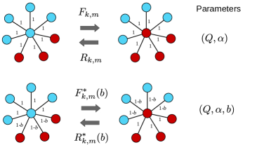
Figure 1: Schematic representation of dynamics of information spreading with a minimal notion of algorithmic bias. With no bias ($b=0$; upper plot), the central node (with degree $k$ and $m$ infected neighbors) interacts with any of its neighbors with probability $1$, regardless of state (denoted by color and shading) and according to transitions rates $F_{k,m}$ and $R_{k,m}$. With bias ($b>0$; lower plot), the node interacts with any of its neighbors in the opposite state with probability $1-b$, resulting in bias-dependent effective rates [$F_{k,m}^{*}(b)$ and $R_{k,m}^{*}(b)$]. The dynamics is determined by noise $Q$ and a parameter $\alpha$ regulating pairwise and group interactions.

Model	$F_{k,m}$	$R_{k,m}$	Phenomenology
Noisy voter [37, 38]	$Q+(1-2Q)\dfrac{m}{k}$	$Q+(1-2Q)\dfrac{k-m}{k}$	$\begin{array}[]{l}\text{ }\\ \text{No transition }(Q>0)\\ \text{ }\end{array}$
Language [40, 41, 42, 43, 44, 45]	$Q+(1-2Q)\left(\dfrac{m}{k}\right)^{\alpha}$	$Q+(1-2Q)\left(\dfrac{k-m}{k}\right)^{\alpha}$	$\begin{array}[]{l}\text{No transition }(\alpha\leq 1)\\ \text{Continuous transition }(1<\alpha\leq 5)\\ \text{Discontinuous transition }(\alpha>5)\\ \end{array}$
Majority-vote [39]	$\begin{cases}Q\hskip 5.69046pt&\text{if}\hskip 14.22636ptm<k/2\\ 1/2\hskip 5.69046pt&\text{if}\hskip 14.22636ptm=k/2\\ 1-Q\hskip 5.69046pt&\text{if}\hskip 14.22636ptm>k/2\end{cases}$	$\begin{cases}1-Q\hskip 5.69046pt&\text{if}\hskip 14.22636ptm<k/2\\ 1/2\hskip 5.69046pt&\text{if}\hskip 14.22636ptm=k/2\\ Q\hskip 5.69046pt&\text{if}\hskip 14.22636ptm>k/2\end{cases}$	$\begin{array}[]{l}\vspace{0.2cm}\\ \text{Continuous transition}\\ \vspace{0.2cm}\end{array}$

Table 1: Models considered in this work, along with references, transition rates ($F_{k,m}$ and $R_{k,m}$) and basic phenomenology of the coexistence-consensus transition in the mean-field limit (complete graph).

We focus our attention on binary-state dynamics with up-down symmetry,

$$R_{k,m}=F_{k,k-m},$$ (1)

meaning the probability to change state is a function of the number of neighbors in the opposite state, regardless of state. From this family we consider three prototypical opinion dynamics: the noisy voter, language, and majority-vote models (Table 1). All models include the parameter $Q\in[0,1/2]$ (with $Q=F_{k,0}=R_{k,k}$), commonly interpreted as noise, ‘social temperature’, or ‘independence’ [46, 47, 44], and equal to the probability of changing state when all neighbors have the same (opposite) opinion. The three models differ in their infection rate $F_{k,m}$: (i) the noisy voter model has a linear dependence on the fraction of infected neighbors $m/k$, corresponding to a pairwise copying mechanism or blind imitation; (ii) the majority-vote model considers that individuals copy the majority state in their neighborhood; and (iii) the language model introduces a non-linear dependence $(m/k)^{\alpha}$ regulated by a tuning parameter $\alpha\in(0,\infty)$. For integer $\alpha$, the language model is driven by group interactions between an individual and $\alpha$ of its neighbors, and opinion unanimity in the group is required to change state. This particular case is also known as the $q-$voter model [41, 43, 47, 48] (with $q=\alpha$). For $\alpha=1$, the language model recovers the noisy voter model and its pairwise interactions.

In many cases the models show a symmetry-breaking phase transition as a function of the noise parameter $Q$, usually between stationary states of opinion consensus [$\rho(t)\neq 1/2$] and coexistence [$\rho(t)=1/2$] for $t\rightarrow\infty$ (see Table 1). The phenomenology of the transition depends on the model. We differentiate between two general behaviors, voter like and majority-vote like [49], with the language model interpolating between the two. For example, in the mean-field limit we can tune $\alpha$ and move from voter like behavior (low $\alpha\lesssim 1$; pairwise interactions), to majority-vote like (high $\alpha\leq 5$; group interactions). In the regime $\alpha>5$ the transition is always discontinuous. This classification, although qualitative, will help us further understand the phenomenology of information spreading for varying $\alpha$ in the presence of algorithmic bias.

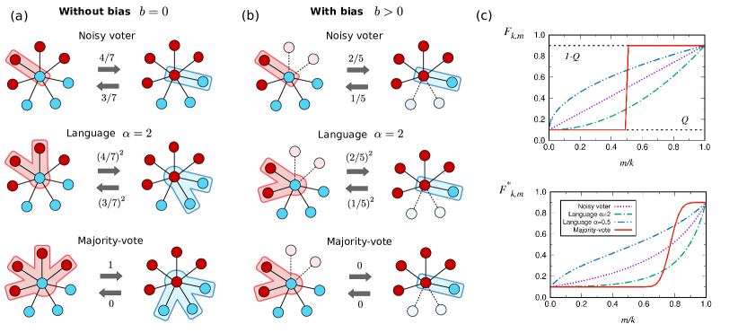
Figure 2: Schematic representation of the considered binary-state dynamics of opinion formation, both in the absence ($b=0$; a) and presence ($b>0$; b) of algorithmic bias. The central node interacts with a set of neighbors (shaded area), ranging from pairwise to group interactions (top to bottom), leading to original/effective transition rates between states (denoted by numbers). In the presence of bias, some neighbors in the opposite state are not considered (dashed links). In (c) we show the functional form of the original ($F_{k,m}$; top) and effective ($F_{k,m}^{*}(b)$; bottom) infection rates as a function of the fraction of infected neighbors $m/k$ for all models, with bias intensity $b=0$ and $b=0.7$, respectively, degree $k=40$ and $Q=0.1$.

II.2 Algorithmic bias

Online platforms use content filtering algorithms, particularly semantic and collaborative filtering [12, 13], to preferably display content similar to what an individual (or alike users) have consumed before, leading to algorithmic bias [14, 15]. In the context of binary-state dynamics of information spreading over social networks, we can minimally implement this bias as a tunable preference to filter the interactions between an individual and its neighbors, depending on their state. We introduce the bias intensity $b$, defined as the probability that a node does not interact with a neighbor in the opposite state (due to content filtering by the platform). If the dynamics is originally driven by rates $F_{k,m}$ and $R_{k,m}$, bias leads to the effective transition rates

$$F_{k,m}^{*}(b)=\sum_{i=0}^{m}B_{m,i}(1-b)F_{k-m+i,i},$$ (2)

$$R_{k,m}^{*}(b)=\sum_{s=0}^{k-m}B_{k-m,s}(1-b)R_{m+s,m},$$ (3)

where $B_{m,i}(1-b)=\binom{m}{i}(1-b)^{i}b^{m-i}$ is the binomial distribution. Eqs. (2)-(3) are simply the average transition rates after removing a number of randomly selected neighbors in the opposite state with probability $b$. Within our framework, the effects of algorithmic bias amount to a binary-state dynamics driven by the effective rates $F_{k,m}^{*}(b)$ and $R_{k,m}^{*}(b)$. Note that this definition of bias respects up-down symmetry [Eq. (1)], since $R_{k,m}^{*}(b)=F^{*}_{k,k-m}(b)$. In general, it is not possible to obtain a simple closed expression for the effective rates of the models listed in Table 1. In Fig. 2 we show a schematic representation of the effect of algorithmic bias on the considered models, together with the shape of the original and effective transition rates as a function of the fraction of infected neighbors $m/k$. In the presence of bias ($b>0$), the language model has effective rates similar to the original rates for a higher value of $\alpha$. Since algorithmic bias ‘hides’ neighbors in the opposite state, more such neighbors are needed for an individual to change state (i.e. a higher $\alpha$ value in the original dynamics). Overall we have $F_{k,m}^{*}(b)\leq F_{k,m}$, meaning bias impedes interactions between individuals that result in a change of opinion. This property is valid for monotonically increasing rates, as $i/(k-m+i)\leq m/k$ for $i=0,\dots,m$ in Eq. (2).

III Methods

III.1 Numerical simulations

The most direct implementation of our framework is by numerical simulation of the stochastic rules described in Section II. At time $t$ of the simulation we perform the following steps: (i) Select an individual $i$ uniformly at random from all $N$ nodes, which has degree $k$ and number of infected neighbors $m$ at time $t$. (ii) If $s_{i}=0$ the individual switches state with probability $F_{k,m}^{*}$, and if $s_{i}=1$ with probability $R_{k,m}^{*}$ . (iii) Time increases by $\Delta t=1/N$ (i.e. the time unit is one Monte Carlo step per node). This numerical method allows us to obtain trajectories of the state variables $\{s_{i}(t)\}_{i=1,\dots,N}$ and consequently the global state $\rho(t)$. We may then compute the average $\langle\rho(t)\rangle$ over stochastic realizations of the same initial conditions, as typically done in non-equilibrium ensembles (in what follows we drop the average brackets for simplicity of notation, unless otherwise stated).

III.2 Mean-field description

III.2.1 Homogeneous network structure

In the simplest analytical treatment of binary-state dynamics, we assume that one dynamical variable is sufficient to describe the state of the system: the global opinion (or fraction of infected nodes) $\rho(t)$. Following the heterogeneous mean-field approximation [31, 24], we obtain a closed differential equation for the dynamics by defining the average rate $f$ of switching state from $0$ to $1$. In the absence of algorithmic bias ($b=0$),

$$f[x]\equiv\sum_{k}\frac{P_{k}k}{z}\sum_{m=0}^{k}F_{k,m}B_{k,m}(x),$$ (4)

where $P_{k}$ is the degree distribution of the network, $z=\sum_{k}P_{k}k$ is the average degree, and $x$ is the probability of finding a neighbor in state $1$. If we consider a homogeneous, highly connected network with $z\gg 1$ (i.e. $P_{k}$ peaks around a high degree), then the binomial function $B_{k,m}(x)$ is also highly peaked around a large $m=zx$. Since the transition rates of the models in Table 1 only depend on the fraction of infected nodes $m/k$, we have $f[m/k]\approx F_{k,m}$. As we approach the mean-field limit, we replace the local (node) probability $x$ of finding a neighbor in state $1$ by the fraction of infected nodes in the network, $\rho$. In the presence of algorithmic bias ($b>0$), Eq. (2) and the assumption of a highly connected network lead to $F^{*}_{k,m}\approx F_{k-bm,(1-b)m}$. The biased version of Eq. (4) is then $f^{*}[x]=f\left[(1-b)x/(1-bx)\right]$, which reduces to $f^{*}[x]=f[x]$ for $b=0$.

Taking into account these approximations, we write a differential equation for the average over realizations of the global opinion $\rho(t)$,

$$\frac{d\rho}{dt}=(1-\rho)f\left[\frac{(1-b)\rho}{1-b\rho}\right]-\rho f\left[\frac{(1-b)(1-\rho)}{1-b(1-\rho)}\right],$$ (5)

where we assume that the probability $x$ of finding a neighbor in state $1$ is just the fraction of infected nodes in the network. Eq. (5) can be thought of as a detailed balance condition: the change in time of the fraction of infected nodes $\rho$ is equal to the probability of selecting a susceptible node ($s=0$) times the rate of switching from $0$ to $1$, minus the probability of selecting an infected node ($s=1$) times the rate of switching from $1$ to $0$. A more detailed derivation of Eq. (5), and an analysis of the accuracy of the highly connected approximation, can be found in the Supplemental Material (SM) [51], Sections S1.2.1 and S1.1.

Note that the accuracy of Eq. (5) depends on two assumptions: (i) a highly connected, homogeneous network with $P_{k}$ peaked around a large average degree $z\gg 1$ (exactly valid only in the case of a complete graph with $z=N-1$); and (ii) a negligible role of stochastic finite-size effects, with $\langle\rho(t)^{n}\rangle\approx\langle\rho(t)\rangle^{n}$ for any $n\geq 1$ (valid in the thermodynamic limit $N\rightarrow\infty$).

III.2.2 Modular network structure

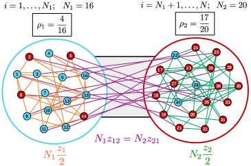
Figure 3: Schematic representation of a simple network with modular (community) structure. Groups 1 and 2 have sizes $N_{1}$ and $N_{2}$, internal average degrees $z_{1}$ and $z_{2}$, are connected between them with average degrees $z_{12}$ and $z_{21}$, and have fractions of infected nodes $\rho_{1}$ and $\rho_{2}$, respectively.

Beyond the degree distribution $P_{k}$, we expect the modular structure of the network to have a major impact on opinion dynamics under the effect of algorithmic bias. In the simplest modular setting, we consider two communities (denoted $1$ and $2$) of sizes $N_{1}$ and $N_{2}$, respectively, with $N=N_{1}+N_{2}$, such that nodes $i=1,\dots,N_{1}$ are in group $1$, and nodes $i=N_{1}+1,\dots,N$ belong to group $2$. We define the internal average degree as the average number of links of a node with others in the same community, $z_{1}=N_{1}^{-1}\sum_{i=1}^{N_{1}}\sum_{j=1}^{N_{1}}A_{ij}$ and $z_{2}=N_{2}^{-1}\sum_{i=N_{1}+1}^{N}\sum_{j=N_{1}+1}^{N}A_{ij}$. The average degree of a node in group 1 with nodes in group 2 is $z_{12}=N_{1}^{-1}\sum_{i=1}^{N_{1}}\sum_{j=N_{1}+1}^{N}A_{ij}$, while the average degree of a node in group 2 with nodes in group 1 is $z_{21}=N_{2}^{-1}\sum_{i=N_{1}+1}^{N}\sum_{j=1}^{N_{1}}A_{ij}$. Since the network is undirected and the adjacency matrix is symmetric ($A_{ij}=A_{ji}$), we have the constraint $N_{1}z_{12}=N_{2}z_{21}$. Just as before, we characterize the state of the system by the fraction of infected nodes in each community, $\rho_{1}(t)=N_{1}^{-1}\sum_{i=1}^{N_{1}}s_{i}(t)$ and $\rho_{2}(t)=N_{2}^{-1}\sum_{i=N_{1}+1}^{N}s_{i}(t)$, with $\rho(t)=\dfrac{N_{1}}{N}\rho_{1}(t)+\dfrac{N_{2}}{N}\rho_{2}(t)$ (see Fig. 3 for a schematic of these definitions and a simple example).

If, at some instant of time, the system is in a non-homogeneous state ($\rho_{1}\neq\rho_{2}$), the probabilities $x_{1}$ and $x_{2}$ of a node in group 1 or 2 finding an infected neighbor ($s=1$) are in principle different and calculated as

$$x_{1}=\frac{N_{1}z_{1}\rho_{1}+N_{2}z_{21}\rho_{2}}{N_{1}z_{1}+N_{2}z_{21}}=\frac{\rho_{1}+p_{1}\rho_{2}}{1+p_{1}},$$ (6)

with $p_{1}=N_{2}z_{21}/N_{1}z_{1}=z_{12}/z_{1}$, and equivalently for $x_{2}$ by exchanging the index $1$ with $2$, i.e., $p_{2}=N_{1}z_{12}/N_{2}z_{2}=z_{21}/z_{2}$. Eq. (6) is the ratio of the number of links coming out of infected nodes that end in community $1$ to the total number of links ending in community $1$. In the homogeneous case where $\rho=\rho_{1}=\rho_{2}$ (i.e. $p_{1}=p_{2}=1$), we recover $x=x_{1}=x_{2}=\rho$ as expected. We write the mean-field rate equations analogous to Eq. (5) by considering the variables $\rho_{1}$ and $\rho_{2}$ and probabilities $x_{1}$ and $x_{2}$,

$$\frac{d\rho_{1}}{dt} =(1-\rho_{1})f\left[\dfrac{(1-b)(\rho_{1}+p_{1}\rho_{2})}{1+p_{1}-b(\rho_{1}+p_{1}\rho_{2})}\right]-\rho_{1}f\left[\dfrac{(1-b)(1-\rho_{1}+p_{1}(1-\rho_{2}))}{1+p_{1}-b(1-\rho_{1}+p_{1}(1-\rho_{2}))}\right],$$ (7)

$$\frac{d\rho_{2}}{dt} =(1-\rho_{2})f\left[\dfrac{(1-b)(\rho_{2}+p_{2}\rho_{1})}{1+p_{2}-b(\rho_{2}+p_{2}\rho_{1})}\right]-\rho_{2}f\left[\dfrac{(1-b)(1-\rho_{2}+p_{2}(1-\rho_{1}))}{1+p_{2}-b(1-\rho_{2}+p_{2}(1-\rho_{1}))}\right],$$ (8)

which reduce to Eq. (5) in the homogeneous case ($\rho_{1}=\rho_{2}=\rho$). A more detailed derivation of Eqs. (7)-(8) can be found in the SM [51], Section S1.2.2.

The solutions $\rho_{1}(t)$ and $\rho_{2}(t)$ of the coupled system in Eqs. (7)-(8) approximate the averages over realizations $\langle\rho_{1}(t)\rangle$ and $\langle\rho_{2}(t)\rangle$ obtained from numerical simulations (see Section III.1). We expect this approximation to be accurate for highly connected networks and large system size $N$. As before, a large average degree is required by the mean-field assumption, and the thermodynamic limit to avoid finite-size effects. The study of Eqs. (7)-(8) will shed light on the dynamics of collective information spreading in the presence of algorithmic bias and the phenomenology of the models considered here.

The dynamics of $\rho_{1}(t)$ and $\rho_{2}(t)$ is completely determined by the parameters $(Q,\alpha,b)$ and initial conditions $\rho_{1}(0)$ and $\rho_{2}(0)$. In order to understand the macroscopic behavior of the models for all parameter values, we build a phase diagram, i.e. we divide the parameter space $(Q,\alpha,b)$ in regions associated with different stable fixed points $\rho_{1}(t)=\rho_{1}^{\text{st}}$ and $\rho_{2}(t)=\rho_{2}^{\text{st}}$. The role of initial conditions can be determined by a vector field or phase portrait, i.e. the right hand side of Eqs. (7)-(8) as a function of $\rho_{1}$ and $\rho_{2}$. The basin of attraction of a stable fixed point delimits the region of initial conditions that will be attracted to that point by the dynamics after long times. Before analyzing the phase diagrams and basins of attraction of all stable fixed points in Section IV, we briefly discuss analytical approximations more accurate than the mean-field limit.

III.3 Higher-order approximations

Higher-order descriptions of binary-state dynamics are possible, at the expense of simplicity and tractability, by considering a set of deterministic evolution equations larger than Eq. (5) or Eqs. (7)-(8), see Section S2 of the SM [51]. In the highly-connected, infinite network size limit the results of all approximations coincide. Higher-order approximations involve evolution equations for random (uncorrelated) networks with an arbitrary degree distribution $P_{k}$, with degrees in the range $k_{\text{min}}\leq k\leq k_{\text{max}}$, and include: (i) the pair approximation [32, 52, 48], with $k_{\text{max}}-k_{\text{min}}+2$ variables, and (ii) approximate master equations [34, 24, 35, 2, 36, 29, 53], with $(1+k_{\text{max}}-k_{\text{min}})(2+k_{\text{max}}+k_{\text{min}})$ variables. In the case of a homogeneous (single community) network structure, the methods developed in the references above can be directly applied to any binary-state model with effective transition rates $F^{*}_{k,m}$ and $R^{*}_{k,m}$ [see Eqs. (2)-(3)]. In the case of modular networks some modifications are needed, as described in the SM [51], Section S2.2, where we develop a pair approximation scheme for modular $z-$regular networks.

IV Theoretical results

We now proceed with a detailed analysis of the fixed points (steady states) of the dynamical mean-field Eqs. (7)-(8) and their stability, in both the absence and presence of algorithmic bias. We first discuss the homogeneous solution $\rho=\rho_{1}=\rho_{2}$ (Section IV.1 and Section S3.1 in the SM [51]), where we focus on the coexistence-consensus transition with order parameter $|\rho-1/2|$, and then turn our attention to the polarized solutions $\rho_{1}\neq\rho_{2}$ (Section IV.2 and Section S3.2 in the SM [51]), where we concentrate on a polarization transition with order parameter $P=|\rho_{1}-\rho_{2}|$.

IV.1 Homogeneous solutions

The homogeneous condition $\rho_{1}(t)=\rho_{2}(t)=\rho(t)$ can be satisfied by Eqs. (7)-(8). Among all possible homogeneous solutions of Eq. (5), we highlight the state of opinion coexistence ($\rho=1/2$), which is always present independently of parameter values as a consequence of the up-down symmetry in the transition rates [see Eq. (1)]. In order to understand the effect algorithmic bias has on these homogeneous solutions, we divide the following results in the cases $b=0$ and $b>0$.

IV.1.1 No algorithmic bias ($b=0$)

In the noisy voter model with $Q>0$, the only stable solution is coexistence ($\rho_{\text{st}}=1/2$) [45, 52]. In the majority-vote model, however, there is a well-defined continuous coexistence-consensus transition (supercritical pitchfork bifurcation) for a finite critical value of the noise $Q_{c}>0$: For $Q>Q_{c}$ the coexistence state $\rho_{\text{st}}=1/2$ is the only stable solution, while for $Q<Q_{c}$ the coexistence state loses its stability and two symmetry-breaking, imperfect consensus states appear as stable solutions, with $|\rho_{\text{st}}-1/2|\propto(Q_{c}-Q)^{1/2}$.

In the language model, for $\alpha\leq 1$ there is no transition and the only stable state is coexistence (like in the noisy voter model). For $1<\alpha<5$ there is a continuous coexistence-consensus transition (supercritical pitchfork bifurcation, majority-vote like), while for $\alpha>5$ the transition is discontinuous (subcritical pitchfork bifurcation). These regimes are separated by a tricritical point at $\alpha=5$. For the discontinuous case there are two transition lines at $Q=Q_{c},Q_{t}$. For $Q>Q_{t}$ the coexistence state is the only stable solution. For $Q_{c}<Q<Q_{t}$ both coexistence and consensus are stable solutions (with a stationary state depending on initial conditions), while for $Q<Q_{c}$ only consensus is possible. In Fig. 4 we show the transition lines $Q=Q_{c},Q_{t}$ as a function of $\alpha$, as well as the stable solutions in the parameter regions $(Q,\alpha)$ delimited by these transition lines (see Refs. [45, 52] for more details on the case without bias, and Table 1 for a summary of the phenomenology).

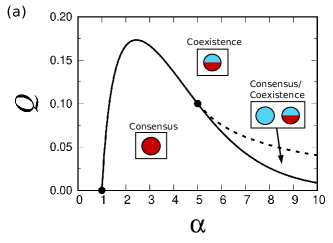
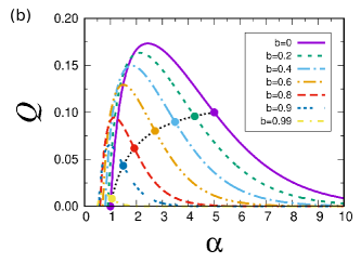
Figure 4: Phase diagram of homogeneous solutions for the language model in parameter space $(Q,\alpha)$, both without bias ($b=0$; a) and for increasing bias in the range $b\in[0,1)$ (b). The solid line in (a) and the different dashed lines in (b) denote the transition values $Q_{c}(\alpha,b)$, while the dashed line in (a) corresponds to $Q_{t}(\alpha,b)$. The tricritical points $\alpha_{t}(0)=5$ and $\alpha_{t}(b)$ [dot in (a) and dotted line in (b), respectively] separate the continuous transition [$1<\alpha<\alpha_{t}(b)$] from the discontinuous [$\alpha>\alpha_{t}(b)$]. Symbols inside squares indicate the global stable states that can be found inside the parameter region delimited by the transition lines. Circle colors (shading in grayscale) correspond to opinion states ($s=0,1$), while a single circle represents a homogeneous system. There are two possible global states: (i) coexistence (mixed-color circles) and (ii) consensus (single-color circles). When more than one stable state is present in a parameter region, the initial condition determines the final state. Note that symmetric states (obtained by exchanging circle colors) are always possible in the same parameter region. The method to obtain the transition parameter values $Q_{c},Q_{t}$ is discussed in the SM [51], Section S3.1.

IV.1.2 Algorithmic bias ($b>0$)

The presence of algorithmic bias (coded by a nonzero intensity $b$) shifts the transition lines and changes their nature. In Fig. 5 we plot the phase diagrams of the three models in Table 1 as a function of $b$. For the noisy voter model, there is always a well defined continuous coexistence-consensus transition for $b>0$. The critical value $Q_{c}$ increases as a function of $b$ up to a maximum at $b=2/3$, after which it decreases to $Q_{c}=0$ for $b=1$. This means that for $b<2/3$, algorithmic bias promotes consensus of opinions in the noisy voter model.

In the majority-vote model, surprisingly, the opposite effect takes place, i.e. the critical point $Q_{c}$ decreases as a function of $b$. In other words, algorithmic bias promotes coexistence of opinions. For high values of $b$ the transition becomes discontinuous with the appearance of a tricritical point, similarly to the phenomenology of the language model without bias for $\alpha>5$ (see Fig. 5). The majority-vote model with high bias thus behaves similarly to the language model with large $\alpha>5$.

The language model, depending on whether $\alpha$ is small or large, interpolates between the two behaviors described above, i.e. algorithmic bias promotes consensus (low $\alpha$) or opinion coexistence (high $\alpha$). With respect to the effect of bias, we can distinguish between voter like (low $\alpha$) and majority-vote like (high $\alpha\leq 5$) behavior. For $\alpha>5$ the transition is always discontinuous with and without bias (see SM [51], Section S3.3 and Fig. S2). We also observe that for high enough bias the transition becomes discontinuous for $1<\alpha<5$, so bias also favors the discontinuity of the transition.

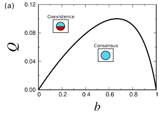
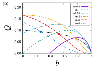
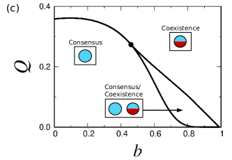
Figure 5: Phase diagrams in parameter space $(Q,b)$ of the homogeneous solutions for the noisy voter (a), language (b), and majority-vote (c) models under algorithmic bias ($b>0$). For the noisy voter and language models, the average rates used to obtain the transition lines are calculated via Eq. (4) in the highly connected limit ($z\rightarrow\infty$), while for the majority-vote model we use a $z-$regular network ($P_{k}=\delta_{k,z}$ with average degree $z=20$). Terminology and symbols are the same as in Fig. 4.

IV.2 Polarized solutions

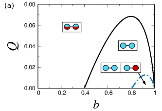
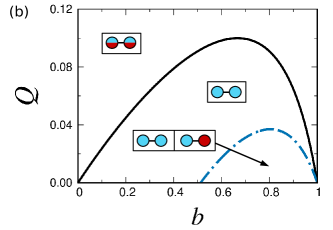
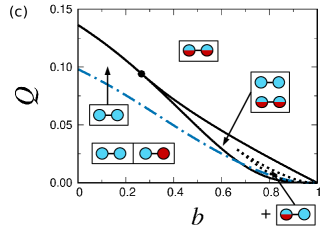
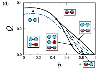
Figure 6: Phase diagrams, in noise-bias parameter space $(Q,b)$, of homogeneous and polarized solutions for the language model with low $\alpha=0.8$ (a), noisy voter model (b), language model with high $\alpha=4$ (c), and majority-vote model (d) in the presence of algorithmic bias and modular network structure (with fixed $p=0.1$), where the order implies a gradual move from pairwise to group interactions. We observe two polarized states: (i) standard polarization (circles of different color; delimited by a dash-dotted line), and (ii) partial polarization (circles with mixed and full colors, delimited by a black dotted line). Symmetric states (obtained by exchanging colors) are always possible in the same parameter region. The stationary state ($t\rightarrow\infty$) in a parameter region with several possible stable states is determined by the initial condition (see Fig. 7). For the noisy voter and language models, average rates used to obtain the transition lines are calculated via Eq. (4) in the highly connected limit ($z\rightarrow\infty$), while for the majority-vote model we use a $z-$regular network ($P_{k}=\delta_{k,z}$ with average degree $z=20$). The method to obtain the transition parameter values $Q^{*}_{p}$ and $Q_{p}$ is described in the SM [51], Section S3.2.

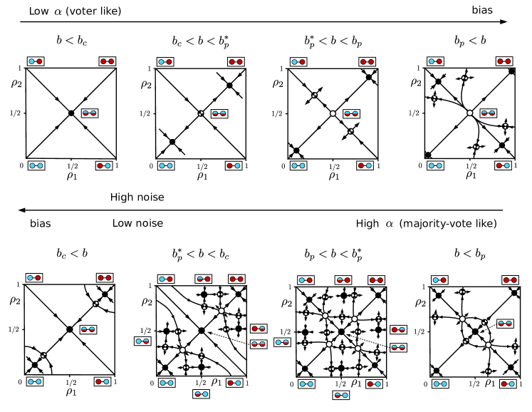
Figure 7: Schematic representation of the various fixed points, linear stability and shape of associated vector fields for Eqs. (7)-(8), a mean-field approximation of binary-state dynamics of information spreading under algorithmic bias. We show all possible phases included in Fig. 6, together with phase transitions that occur for fixed noise $Q$ and varying bias intensity $b$ (examples of the associated vectors fields for given values of the parameters can be found in SM [51], Section S3.4).

In order to understand the interplay between algorithmic bias and modular network structure in binary dynamics of information spreading, we relax the homogeneous condition and allow $\rho_{1}$ and $\rho_{2}$ to vary freely. Solutions that do not fulfill the condition $\rho_{1}=\rho_{2}$ can be considered as polarized, since groups have different average opinions. Extreme polarization happens for $\rho_{1}=1$ and $\rho_{2}=0$ (or the other way around), i.e. full consensus in community $1$ and full consensus of the opposite opinion in community $2$. We measure the degree of polarization in the social system with the order parameter $P=|\rho_{1}-\rho_{2}|\in[0,1]$, such that the homogeneous case ($\rho_{1}=\rho_{2}$) corresponds to $P=0$, and extreme polarization to $P=1$. Any other value ($0<P<1$) represents polarization to a certain degree.

Assuming communities of equal size ($N_{1}=N_{2}=N/2$) and connectivity ($z_{1}=z_{2}$, $p=p_{1}=p_{2}=z_{12}/z_{1}=z_{21}/z_{2}$), it is straightforward to show that a possible solution of Eqs. (7)-(8) fulfills the condition $\rho_{1}(t)+\rho_{2}(t)=1$, which we call the polarization line. We are mainly interested in stationary solutions across this line, but there are polarized solutions outside of it. Note that even if we find a fixed point in the polarization line, stability analysis needs to be performed in all directions, not only across the line.

In all considered models, for particular values of the noise $Q$, bias intensity $b$, and connectivity parameter $p$, we find a transition to polarization. If we vary the noise $Q$ and keep other parameters fixed, there are two critical values: $Q_{p}$ and $Q^{*}_{p}$ with $Q_{p}<Q^{*}_{p}$. For $Q>Q^{*}_{p}$, there are no fixed points along the polarization line besides the trivial coexistence state $\rho_{1}^{\text{st}}=\rho_{2}^{\text{st}}=1/2$. For $Q_{p}<Q<Q^{*}_{p}$ two polarized fixed points appear, stable along the polarization line and unstable in the perpendicular direction (the homogeneous line), meaning they are saddle points in $(\rho_{1},\rho_{2})$ space. For $Q<Q_{p}$ the same fixed points become stable in both directions, representing a polarized state of opinion.

The polarization transition line $Q_{p}(\alpha,b,p)$, or equivalently $b_{p}(Q,\alpha,p)$, is displayed in Fig. 6 for all models. In Fig. 7 we show a schematic representation of the fixed points and their stability analysis, i.e. the phase portrait, of all phases in Fig. 6. We summarize the behavior of the polarization transition in each model as follows.

In the noisy voter model, the polarization transition appears for a fixed value of the bias intensity $b>b_{p}(0,1,p)$, while for $b<b_{p}(0,1,p)$ the polarized state disappears. This means that polarization emerges as a consequence of algorithmic bias. The noise value at the transition $Q_{p}(1,b,p)$ increases as a function of $b$ and has a maximum, similarly to the homogeneous coexistence-consensus transition line. Overall, polarization is induced and promoted by algorithmic bias in the presence of pairwise interactions.

In the majority-vote model, polarization already exists without bias ($b=0$). As bias increases, the transition value $Q_{p}$ changes slightly (the transition line is very flat as a function of $b$) and may have a small maximum depending on $p$. For high enough bias $Q_{p}(b,p)$ decreases, meaning that bias may inhibit polarization, as opposed to the noisy voter model. For large $b$ a new stable polarized state appears, where one of the groups has consensus and the other one coexistence. This new state is possible because consensus and coexistence are both stable in the homogeneous phase. In Fig. 6, inside the consensus/coexistence region of the homogeneous phase, we observe a smaller region where the new state is stable. In Fig. 7 we show how these new states appear, together with the stability analysis of all additional fixed points outside of the polarization line.

The behavior of the language model depends on the value of $\alpha$, as before. For low values, we find similar behavior as the noisy voter model with an emergence of polarization for increasing bias. High values of $\alpha$ display the opposite behavior, with polarization disappearing for large enough $b$, similarly to the majority-vote model. Note that the previous statements and the results of Fig. 6 correspond to a fixed value of the connectivity parameter $p$. The polarization transition lines strongly depend on the value of $p$. For example, the value of $\alpha$ that separates (smoothly) voter like and majority-voter like behaviors increases with $p$. If the value of $p$ is high enough, but a polarized solution still exists despite the high degree of mixing between groups, the polarization transition has a maximum as function of $b$, even for large $\alpha$ (for more details on the separation between $\alpha$ regimes see SM [51], Section S3.3 and Fig. S2).

V Comparison with numerical simulations

In Section IV we have derived analytical approximations for binary-state dynamics with algorithmic bias (for both homogeneous and modular networks) in terms of mean-field equations, which allow us to characterize the behavior of specific opinion formation models as a function of parameters $(Q,\alpha,b,p)$. In what follows we validate these theoretical results with numerical simulations in synthetic and real networks.

V.1 Synthetic networks

Synthetic networks with heterogeneous, uncorrelated degrees and modular structure can be generated by using the configuration model [54], where we take as input degree sequences and the community each node belongs to (see, e.g., Fig. 3). We use the generated networks for numerical simulations and compute the corresponding pair approximation (a more accurate analytical description developed in SM [51], Section S2). In the case of homogeneous networks, we also solve the associated approximate master equations [24] numerically. We then compare these results with the mean-field Eqs. (7)-(8) to test the validity of the highly connected limit.

Comparing the pair approximation with the mean-field results (see Fig. 6), we find the same qualitative behavior in networks with finite average degrees $z_{1}$, $z_{12}$, $z_{2}$, and $z_{21}$, with the same type of transitions. The transition lines shift, however, and the critical values depend on the connectivity parameters. In the pair approximation, the critical noise at the transition is smaller than in the mean-field case, and the network tends to destroy the discontinuous transition, reducing the parameter region where it can be found. For networks with $z\leq 5$, the discontinuous transition disappears completely. Something similar happens with the polarization transition; a network with finite connectivity reduces the parameter region where the polarized state can be found, as compared to the mean-field limit with the same $p$ value. For extremely sparse networks the polarized state disappears (see SM [51], Section S4 and Fig. S9 in the case $z_{12}=1$ and $z_{1}=5$, $p=0.2$). In the SM we show how the network affects the transition values $Q_{c}$ and $Q_{p}$ for given model parameters and as a function of the connectivity $z_{1}$. Note that we vary the value of $z_{1}$ but keep $p=z_{12}/z_{1}$ ($N_{1}=N_{2}$) constant so that the mean-field results are independent of $z_{1}$. As shown in the SM [51], Section S4, Fig. S9 and Fig. S11, the pair approximation is very accurate for the language model with $\alpha=2$ as compared to numerical simulations on $z-$regular networks with community structure, and we recover the mean-field limit for $z_{1}\rightarrow\infty$. In this case, the transition parameter values predicted by the pair approximation fall within error bars of computer simulations, thus validating our analytical results.

While the accuracy of the pair approximation is remarkable in most cases of interest, some discrepancies appear for high $\alpha\gtrsim z$, for extremely sparse networks ($z\approx 2$), and for the majority-vote model with large bias (see SM [51], Fig. S10 and Fig. S12). These discrepancies are corrected by the approximate master equations, which predict the transition values within the error range of numerical simulations for all parameter values and models considered.

V.2 Real-world social networks

Apart from heterogeneous degrees and a potentially stylized modular structure, real-world networks display higher-order (e.g., degree-degree) correlations and other mesoscopic properties not considered in the mean-field limit. We check the validity of our theoretical results by performing numerical simulations of the dynamics (see Section III.1) on top of an empirical network structure, confirming that the effect of algorithmic bias on the transitions between coexistence, consensus and polarization is qualitatively the same even in the presence of more involved structural features.

We take the political blogs network [55, 27], where nodes represent liberal and conservative blogs around the time of the 2004 US presidential election. Links exist between blogs that refer to each other often, implying a strong interaction between blogs, i.e. the potential for information spreading. Based on existing metadata, the population can be divided in two groups of sizes $N_{1}=450$ (liberals) and $N_{2}=523$ (conservatives), with $N=N_{1}+N_{2}=973$ (after removing nodes with less than three links). Average degrees inside groups are $z_{1}=31.74$ and $z_{2}=29.37$, and between groups $z_{12}=3.42$ and $z_{21}=2.94$. Thus, the conservative community is larger but less connected than the liberal group. Since average degrees are relatively large, we expect the mean-field Eqs. (7)-(8) (with connectivity parameters $p_{1}=0.1076$ and $p_{2}=0.1001$) to provide accurate results for the dynamics and stationary states of the social system. Note that the values of parameters $p_{1}$ and $p_{2}$ indicate that an individual in group $1$ (liberal) is (slightly) more likely to be convinced by an individual in group $2$ (conservative) than the other way around, suggesting that opinion dynamics might be driven by the conservative group.

We perform numerical simulations of the stochastic opinion dynamics using the noisy voter model with noise value $Q=0.01$ and a high bias intensity ($b=0.8$), which is close to the polarization maximum (see Fig. 6). According to the mean-field theory there are two (symmetric and stable) polarized states with $\rho_{1}^{\text{st}}=0.09$, $\rho_{2}^{\text{st}}=0.92$, and global opinion $\rho_{\text{st}}=0.54$ (or $\rho_{1}^{\text{st}}=0.91$, $\rho_{2}^{\text{st}}=0.08$, and global opinion $\rho_{\text{st}}=0.46$). Note that opinion consensus in group $1$ is always weaker than in group $2$, a consequence of the asymmetry in group size and connectivity. Linear stability analysis determines that the polarized state is stable with eigenvalues and eigenvectors $\lambda_{1}=-0.16$, $\vec{v}_{1}=\begin{bmatrix}0.86\\ 0.51\end{bmatrix}$, and $\lambda_{2}=-0.24$, $\vec{v}_{2}=\begin{bmatrix}-0.55\\ 0.84\end{bmatrix}$. There is a slow and a fast eigendirection, which means that the approach to the polarized state happens first in group $2$ ($\rho_{2}(t)\rightarrow\rho_{2}^{\text{st}}$), and afterwards in group $1$ ($\rho_{1}(t)\rightarrow\rho_{1}^{\text{st}}$). This also implies that group 1 is less resilient and more vulnerable to perturbations, dynamical fluctuations in the slow eigendirection will have a larger amplitude, and thus opinions will vary more in time.

In Fig. 8 we compare the vector field of the mean-field theory [coming from Eqs. (7)-(8)] to single trajectories $\rho_{1}(t)$, $\rho_{2}(t)$ of numerical simulations with several initial conditions, as well as to restricted averages over realizations that end up in the same final state $\langle\rho_{1}(t)\rangle$, $\langle\rho_{2}(t)\rangle$. Numerical average values agree considerably well with the vector field of the theory, and also converge to the predicted final state, indicating that in the case of the political blogs network, a simple mean-field description is sufficient to describe the dynamical and stationary properties of binary-state information spreading under the effect of bias.

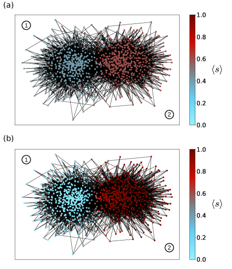
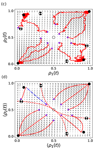
Figure 8: Mean-field vector fields Eqs. (7)-(8) together with single trajectories (c) and average values over realizations (d) (solid lines) coming from numerical simulations of the noisy voter model in the political blogs network [55, 27] with noise $Q=0.01$ and bias intensity $b=0.8$. Smaller dots are initial conditions, larger filled dots stable fixed points, empty dots unstable fixed points, and half-filled dots saddle points. Dashed lines in (d) delimit the basin of attraction of the polarization and consensus states. The dash-dotted line in (d) is a particular trajectory for which we show the average initial (a) and final (b) states of the simulated opinion dynamics over the empirical network. Node positions are calculated with the Louvain method of community detection.

VI Discussion

Algorithmic bias, an unexpected consequence of the content filtering tools behind most popular social media platforms used today, affects the dynamics of opinion formation and information spreading arising from digital interactions in non-trivial ways, ultimately leading to undesired collective phenomena like group polarization and opinion radicalization [20, 21]. While the role of algorithmic bias has been recently modeled in an array of concrete scenarios [18, 22, 25], a general theoretical framework systematically linking social dynamics, network structure and algorithmic filtering has been missing so far. Here we have put forward such a formalism by extending previous work on binary-state dynamics [34, 24, 35, 2, 45, 36, 29] with a notion of bias and applying it to synthetic and real-world social networks. While our formalism applies to any binary-state dynamics, we have showcased its flexibility by focusing on the noisy voter, language, and majority-vote models, which consider a (pairwise or group-based) copying or herding mechanism, alongside random or idiosyncratic changes of opinion.

We derived a set of deterministic, non-linear rate equations describing the macroscopic dynamics of the system with increasing levels of accuracy: mean-field, pair approximation, and approximate master equations. From these equations we determined the possible stationary states of the dynamics and their stability. We observed a rich phenomenology with respect to various parameters (bias intensity $b$, noise $Q$, model tuning parameter $\alpha$, and inter-group connectivity $p$), including continuous and discontinuous phase transitions between stationary states of consensus, coexistence and polarization.

Algorithmic bias plays a crucial role in the shape of the associated phase diagram. It promotes consensus (in homogeneous networks) and polarization of opinions (in modular networks) when pairwise interactions are predominant (the noisy-voter and language models with low $\alpha$). When the dynamics is driven instead by group-based interactions (majority-vote and language models with high $\alpha$), algorithmic bias promotes coexistence of opinions. The role of algorithmic bias on the coexistence-consensus transition has an intuitive interpretation: For pairwise interactions, bias makes it harder for individuals to copy opposing states, thus favoring consensus and polarization of opinions. For group interactions, however, opinion unanimity within a group is necessary for an individual to change state. Under algorithmic bias, the opinion of part of the group is hidden due to content filtering, making majorities harder to form. Fewer state changes due to copying mechanisms and an increasing role of noise leads to coexistence. The separation between pairwise and group based behaviors depends on the specific details of the rates of the model; for the language model the transition occurs smoothly for an intermediate value $\alpha\approx 2$, see Section S3.3 and Figure S2 of the SM [51] for more details. For other binary-state models well-described by local transition rates we expect such a separation to exist (see [56] where these results are extended for asymmetric rates, and pair and group based behaviors are discussed in detail). We leave as further work the extension of our analysis to other opinion formation mechanisms beyond voter-like dynamics.

When algorithmic bias is strong, the coexistence-consensus transition becomes discontinuous. In addition to a ‘standard’ polarized state (where each group is close to consensus in opposite states), for large $b$ and $\alpha$ we observed an additional, ‘half’ polarized state where one group has opinion coexistence and the other one consensus. Note that a wide variety of other unstable or saddle points also exist depending on parameter values and initial conditions, regulating transient states in the dynamics. In most cases, the mean-field approximation presented here gives a good qualitative description of the phase diagram under the effect of algorithmic bias. Using higher-order approximations (pair and approximate master equations) gradually improves accuracy with respect to simulation results. We also explored the role of algorithmic bias in models of opinion dynamics over a real-world social network with strong modular structure, the political blogs network [55]. In the parameter region where the polarized state is stable according to the mean field approximation, numerical simulations converge to a polarization of opinions that corresponds to the structural segregation of the network, provided the initial condition is in the basin of attraction of the associated fixed point. We expect our mean-field results to work similarly well in other empirical networks that are link dense or modular.

Our formalism provides a flexible way to parametrize a combination of algorithmic filters and mechanisms of social interactions in terms of transition rates. As such, it may help identify the features of algorithms that promote dynamical and structural polarization in online platforms arguably driven by a mixture of social processes, from homophily [26, 27] to social contagion [28, 29]. This will require a validation of our theoretical framework by either fitting observational data with specific models, using automatic model selection [57, 58] and statistical inference techniques [59], or uncovering causal relationships with controlled experiments of online social behavior [60, 61].

The minimal implementation of algorithmic bias explored here can be extended to include more realistic traits of current online media platforms, such as an asymmetry in the state favored by bias, correlations between bias and individual traits (like network degree), a combination of potentially competing filtering algorithms, and the presence of algorithms that react adaptively to changes in human behavior. While we have focused on binary-state dynamics of opinion formation due to the simplicity of the related approximations and relevance to online platforms, we expect our framework to be straightforwardly generalized to models with more than two states or even continuous dynamical variables.

A key limitation of our framework is the consideration of static networks only. Real-world online social networks are instead temporal [62], with both nodes and links changing in time due to a variety of mechanisms and external factors influencing how people use media platforms and choose their acquaintances. If extended to temporal networks [29], our framework will potentially describe a feedback loop between algorithmic content filtering and network/state dynamics that segregates the social network into groups of similarly-minded people (as suggested by recent studies [63]), further promoting the polarization effect we already see in static networks. Even if our results focus on binary-state dynamics over simple networks, the rate-equation-based framework is flexible and can be extended to other dynamical descriptions, such as nonlinear dynamical systems with continuous variables [64, 65] and higher-order network models [66].

The theoretical understanding of the dynamical feedback processes between filters, information transfer and network evolution provided by our framework can suggest heuristic techniques to correct bias. For example, promoting group-based information exchange in a platform dominated by pairwise contacts may decrease polarization and allow for coexistence. Such strategies can improve the chances of a population self-identifying the onset of processes that may reduce their robustness to undesired behavior, like the political swaying and polarization promoted by adversarial agents and social bots in online discussion forums [67, 68]. We trust our results will be part of a larger trend providing scientific background for beneficial regulation and rules of practice in online social ecosystems.

Author contributions

All authors conceived and designed the research. A.F.P. derived all analytical calculations, performed numerical simulations, and analyzed the data. M.N. and G.I. derived effective rates in presence of bias. A.F.P., J.K., and G.I. wrote the manuscript. All authors approved the manuscript.

References

- Castellano et al. [2009a] C. Castellano, S. Fortunato, and V. Loreto, Statistical physics of social dynamics, Rev. Mod. Phys. 81, 591 (2009a).
- Porter and Gleeson [2016] M. A. Porter and J. P. Gleeson, Dynamical systems on networks, Front. Appl. Dynam. Syst. 4 (2016).
- Cimini et al. [2019] G. Cimini, T. Squartini, F. Saracco, D. Garlaschelli, A. Gabrielli, and G. Caldarelli, The statistical physics of real-world networks, Nat. Rev. Phys. 1, 58 (2019).
- Newman [2003] M. E. J. Newman, The structure and function of complex networks, SIAM Rev. 45, 167 (2003).
- Boccaletti et al. [2006] S. Boccaletti, V. Latora, Y. Moreno, M. Chavez, and D.-U. Hwang, Complex networks: Structure and dynamics, Phys. Rep. 424, 175 (2006).
- Starnini et al. [2013] M. Starnini, A. Baronchelli, and R. Pastor-Satorras, Modeling human dynamics of face-to-face interaction networks, Phys. Rev. Lett. 110, 168701 (2013).
- Latora et al. [2017] V. Latora, V. Nicosia, and G. Russo, Complex Networks: Principles, Methods and Applications (Cambridge University Press, 2017).
- Lambiotte and Schaub [2021] R. Lambiotte and M. Schaub, Modularity and Dynamics on Complex Networks (Cambridge University Press, 2021).
- Lazer et al. [2009] D. Lazer, A. S. Pentland, L. Adamic, S. Aral, A. L. Barabasi, D. Brewer, N. Christakis, N. Contractor, J. Fowler, M. Gutmann, et al., Computational social science, Science 323, 721 (2009).
- Conte et al. [2012] R. Conte, N. Gilbert, G. Bonelli, C. Cioffi-Revilla, G. Deffuant, J. Kertesz, V. Loreto, S. Moat, J.-P. Nadal, A. Sanchez, et al., Manifesto of computational social science, Eur. Phys. J. Special Topics 214, 325 (2012).
- Nikolov et al. [2018] D. Nikolov, M. Lalmas, A. Flammini, and F. Menczer, Quantifying biases in online information exposure, J. Assoc. Inf. Sci. Tech. 70, 218 (2018).
- Bozdag [2013] E. Bozdag, Bias in algorithmic filtering and personalization, Ethics Inf. Technol. 15, 209 (2013).
- Möller et al. [2018] J. Möller, D. Trilling, N. Helberger, and B. van Es, Do not blame it on the algorithm: an empirical assessment of multiple recommender systems and their impact on content diversity, Inform. Commun. Soc. 21, 959 (2018).
- Pariser [2011] E. Pariser, The Filter Bubble: What The Internet Is Hiding From You (Penguin Books Limited, 2011).
- Bakshy et al. [2015] E. Bakshy, S. Messing, and L. A. Adamic, Exposure to ideologically diverse news and opinion on facebook, Science 348, 1130 (2015).
- Vicario et al. [2016] M. D. Vicario, G. Vivaldo, A. Bessi, F. Zollo, A. Scala, G. Caldarelli, and W. Quattrociocchi, Echo chambers: Emotional contagion and group polarization on facebook, Sci. Rep. 6, 37825 (2016).
- Bail et al. [2018] C. A. Bail, L. P. Argyle, T. W. Brown, J. P. Bumpus, H. Chen, M. F. Hunzaker, J. Lee, M. Mann, F. Merhout, and A. Volfovsky, Exposure to opposing views on social media can increase political polarization, Proc. Nat. Acad. Sci. USA 115, 9216 (2018).
- Ciampaglia et al. [2018] G. L. Ciampaglia, A. Nematzadeh, F. Menczer, and A. Flammini, How algorithmic popularity bias hinders or promotes quality, Sci. Rep. 8, 1 (2018).
- Blex and Yasseri [2020] C. Blex and T. Yasseri, Positive algorithmic bias cannot stop fragmentation in homophilic networks, J. Math. Sociol. 0, 1 (2020).
- Baumann et al. [2020] F. Baumann, P. Lorenz-Spreen, I. M. Sokolov, and M. Starnini, Modeling echo chambers and polarization dynamics in social networks, Phys. Rev. Lett. 124, 048301 (2020).
- Cinelli et al. [2021] M. Cinelli, G. D. F. Morales, A. Galeazzi, W. Quattrociocchi, and M. Starnini, The echo chamber effect on social media, Proc. Nat. Acad. Sci. USA 118, e2023301118 (2021).
- Sîrbu et al. [2019] A. Sîrbu, D. Pedreschi, F. Giannotti, and J. Kertész, Algorithmic bias amplifies opinion fragmentation and polarization: A bounded confidence model, PLoS ONE 14, e0213246 (2019).
- Deffuant et al. [2000] G. Deffuant, D. Neau, F. Amblard, and G. Weisbuch, Mixing beliefs among interacting agents, Adv. Comp. Syst. 03, 87 (2000).
- Gleeson [2013] J. P. Gleeson, Binary-state dynamics on complex networks: Pair approximation and beyond, Phys. Rev. X 3, 021004 (2013).
- Perra and Rocha [2019] N. Perra and L. E. C. Rocha, Modelling opinion dynamics in the age of algorithmic personalisation, Sci. Rep. 9, 7261 (2019).
- McPherson et al. [2001] M. McPherson, L. Smith-Lovin, and J. M. Cook, Birds of a feather: Homophily in social networks, Annu. Rev. Sociol. 27, 415 (2001).
- Asikainen et al. [2020] A. Asikainen, G. Iñiguez, J. Ureña-Carrión, K. Kaski, and M. Kivelä, Cumulative effects of triadic closure and homophily in social networks, Sci. Adv. 6, eaax7310 (2020).
- Watts [2002] D. J. Watts, A simple model of global cascades on random networks, Proc. Nat. Acad. Sci. USA 99, 5766 (2002).
- Unicomb et al. [2021] S. Unicomb, G. Iñiguez, J. P. Gleeson, and M. Karsai, Dynamics of cascades on burstiness-controlled temporal networks, Nat. Comm. 12, 1 (2021).
- Sood et al. [2008] V. Sood, T. Antal, and S. Redner, Voter models on heterogeneous networks, Phys. Rev. E 77, 041121 (2008).
- Vespignani [2012] A. Vespignani, Modelling dynamical processes in complex socio-technical systems, Nat. Phys. 8, 32 (2012).
- Vazquez and Eguíluz [2008] F. Vazquez and V. M. Eguíluz, Analytical solution of the voter model on uncorrelated networks, New J. Phys. 10, 063011 (2008).
- Pugliese and Castellano [2009] E. Pugliese and C. Castellano, Heterogeneous pair approximation for voter models on networks, Europhys. Lett. 88, 58004 (2009).
- Gleeson [2011] J. P. Gleeson, High-accuracy approximation of binary-state dynamics on networks, Phys. Rev. Lett. 107, 068701 (2011).
- Ruan et al. [2015] Z. Ruan, G. Iñiguez, M. Karsai, and J. Kertész, Kinetics of social contagion, Phys. Rev. Lett. 115, 218702 (2015).
- Unicomb et al. [2018] S. Unicomb, G. Iñiguez, and M. Karsai, Threshold driven contagion on weighted networks, Sci. Rep. 8, 3094 (2018).
- Kirman [1993] A. Kirman, Ants, Rationality, and Recruitment*, Q. J. Econ. 108, 137 (1993).
- Granovsky and Madras [1995] B. L. Granovsky and N. Madras, The noisy voter model, Stoch. Proc. Appl. 55, 23 (1995).
- de Oliveira [1992] M. J. de Oliveira, Isotropic majority-vote model on a square lattice, J. Stat. Phys. 66, 273 (1992).
- Abrams and Strogatz [2003] D. Abrams and S. Strogatz, Modelling the dynamics of language death, Nature 424, 900 (2003).
- Castellano et al. [2009b] C. Castellano, M. A. Muñoz, and R. Pastor-Satorras, Nonlinear -voter model, Phys. Rev. E 80, 041129 (2009b).
- Schweitzer and Behera [2009] F. Schweitzer and L. Behera, Nonlinear voter models: the transition from invasion to coexistence, Eur. Phys. J. B 67, 301 (2009).
- Nyczka et al. [2012] P. Nyczka, K. Sznajd-Weron, and J. Cisło, Phase transitions in the -voter model with two types of stochastic driving, Phys. Rev. E 86, 011105 (2012).
- J\polhkedrzejewski [2017] A. J\polhkedrzejewski, Pair approximation for the -voter model with independence on complex networks, Phys. Rev. E 95, 012307 (2017).
- Peralta et al. [2018a] A. F. Peralta, A. Carro, M. San Miguel, and R. Toral, Analytical and numerical study of the non-linear noisy voter on complex networks, Chaos 28, 075516 (2018a).
- Nail et al. [2000] P. R. Nail, G. MacDonald, and D. A. Levy, Proposal of a four-dimensional model of social response., Psychol. Bull. 126, 454 (2000).
- Nyczka and Sznajd-Weron [2013] P. Nyczka and K. Sznajd-Weron, Anticonformity or independence?—insights from statistical physics, J. Stat. Phys. 151, 174 (2013).
- Vieira et al. [2020] A. R. Vieira, A. F. Peralta, R. Toral, M. S. Miguel, and C. Anteneodo, Pair approximation for the noisy threshold -voter model, Phys. Rev. E 101, 052131 (2020).
- Castelló et al. [2006] X. Castelló, V. M. Eguíluz, and M. San Miguel, Ordering dynamics with two non-excluding options: bilingualism in language competition, New J. Phys. 8, 308 (2006).
- Note [1] Note that this requires that the for all nodes (all possible values of and ). If that is not the case, we must re-scale the rates and time dividing by the maximum value .
- Peralta et al. [2021a] A. F. Peralta, M. Neri, J. Kertész, and G. Iñiguez, See supplemental material at [url] for a detailed derivation of the mean field and pair approximation equations, the characterization of the phase transitions and the comparison with numerical simulations (2021a).
- Peralta et al. [2018b] A. F. Peralta, A. Carro, M. San Miguel, and R. Toral, Stochastic pair approximation treatment of the noisy voter model, New J. Phys. 20, 103045 (2018b).
- Peralta and Toral [2020] A. F. Peralta and R. Toral, Binary-state dynamics on complex networks: Stochastic pair approximation and beyond, Phys. Rev. Research 2, 043370 (2020).
- Catanzaro et al. [2005] M. Catanzaro, M. Boguñá, and R. Pastor-Satorras, Generation of uncorrelated random scale-free networks, Phys. Rev. E 71, 027103 (2005).
- Adamic and Glance [2005] L. A. Adamic and N. Glance, The political blogosphere and the 2004 u.s. election: Divided they blog, in Proceedings of the 3rd International Workshop on Link Discovery, LinkKDD ’05 (Association for Computing Machinery, New York, NY, USA, 2005) p. 36–43.
- Peralta et al. [2021b] A. F. Peralta, J. Kertész, and G. Iñiguez, Opinion formation on social networks with algorithmic bias: Dynamics and bias imbalance (2021b), arXiv:2108.01350 [physics.soc-ph] .
- Gutmann and Corander [2016] M. U. Gutmann and J. Corander, Bayesian optimization for likelihood-free inference of simulator-based statistical models, J. Mach. Learn. Res. 17, 4256 (2016).
- Chen et al. [2019] S. Chen, A. Mira, and J.-P. Onnela, Flexible model selection for mechanistic network models, J. Comp. Net. 8 (2019), cnz024.
- Peixoto [2019] T. P. Peixoto, Network reconstruction and community detection from dynamics, Phys. Rev. Lett. 123, 128301 (2019).
- Salganik et al. [2006] M. J. Salganik, P. S. Dodds, and D. J. Watts, Experimental study of inequality and unpredictability in an artificial cultural market, Science 311, 854 (2006).
- Centola [2010] D. Centola, The spread of behavior in an online social network experiment, Science 329, 1194 (2010).
- Holme and Saramäki [2012] P. Holme and J. Saramäki, Temporal networks, Phys. Rep. 519, 97 (2012).
- de Arruda et al. [2021] H. F. de Arruda, F. M. Cardoso, G. F. de Arruda, A. R. Hernández, L. d. F. Costa, and Y. Moreno, Modeling how social network algorithms can influence opinion polarization, Eprint arXiv:2102.00099 (2021).
- Barzel and Barabási [2013] B. Barzel and A.-L. Barabási, Universality in network dynamics, Nat. Phys. 9, 673 (2013).
- Gao et al. [2016] J. Gao, B. Barzel, and A.-L. Barabási, Universal resilience patterns in complex networks, Nature 530, 307 (2016).
- Lambiotte et al. [2019] R. Lambiotte, M. Rosvall, and I. Scholtes, From networks to optimal higher-order models of complex systems, Nat. Phys. 15, 313 (2019).
- Ferrara et al. [2016] E. Ferrara, O. Varol, C. Davis, F. Menczer, and A. Flammini, The rise of social bots, Commun. ACM 59, 96 (2016).
- Bessi and Ferrara [2016] A. Bessi and E. Ferrara, Social bots distort the 2016 us presidential election online discussion, First Monday 21 (2016).