Primordial black holes and secondary gravitational waves from string inspired general no-scale supergravity
Abstract
The formation of primordial black hole (PBH) dark matter and the generation of scalar induced secondary gravitational waves (SIGWs) have been studied in the generic no-scale supergravity inflationary models. By adding an exponential term to the Kähler potential, the inflaton experiences a period of ultraslow-roll and the amplitude of primordial power spectrum at small scales is enhanced to . The enhanced power spectra of primordial curvature perturbations can have both sharp and broad peaks. A wide mass range of PBHs can be produced in our model, and the frequencies of the accompanied SIGWs are ranged form nanohertz to kilohertz. We show four benchmark points where the generated PBH masses are around , , and . The PBHs with masses around and can make up almost all the dark matter, and the accompanied SIGWs can be probed by the upcoming space-based gravitational wave observatory. Also, the SIGWs accompanied with the formation of stellar mass PBHs can be used to interpret the stochastic GW background in the nanohertz band, detected by the North American Nanohertz Observatory for gravitational waves, and can be tested by future interferometric gravitational wave observatory.
I Introduction
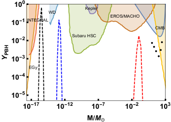
Since the direct detections of gravitational wave (GW) by the Laser Interferometer Gravitational-Wave Observatory (LIGO) Scientific Collaboration and the Virgo Collaboration [1, 2, 3, 4, 5, 6, 7, 8, 9, 10, 11, 12, 13], the idea that primordial black hole (PBH) can be considered as dark matter (DM) candidate [14, 15, 16, 17, 18, 19, 20, 21, 22] has again attracted the attention of physicists and astronomers [23, 24, 25, 26, 27, 28, 29, 30, 31, 32]. The DM fraction in the form of PBHs is tightly constrained by current observations [28, 33, 34], but there is no observational constraint in the mass windows around the masses and , so PBHs with masses around and can account for the total amount of DM.
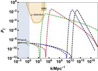
PBHs are formed during radiation domination through gravitational collapse in overdense regions, where the density contrast of small-scale overdense regions at horizon reentry is greater than the threshold value [35, 36]. To produce PBHs during the radiation era, the primordial scalar power spectrum at small scales should be enhanced to [37, 38]. However, the amplitude of the scalar power spectrum at Mpc-1 is constrained to be [39, 40]. Thus, how to enlarge the primordial curvature perturbation at small scales becomes the key to progress. One mechanism to realize the enhancement of the power spectrum is the ultraslow-roll inflation with an inflection point [41, 42, 43, 44, 45, 46, 47, 48, 49, 50, 51, 52, 53, 54, 55, 56]. The other mechanisms rely on a peak function either in the nonminimal coupling or in noncannonical kinetic term [57, 58, 59, 60, 61, 62, 63, 64, 65, 66, 67]. The location of the inflection point or the peak in the primordial scalar power spectrum is crucial for the calculation of the mass and abundance of PBHs. Near the inflection point, the inflaton potential has an extreme flat plateau where the slow-roll parameter becomes very small and the power spectrum amplifies. However, the slow-roll approximation is not satisfied around the point. To describe the precise evolution of the power spectrum, the Mukhanov-Sasaki equation should be numerically solved for each mode [68].
Since the scalar perturbations and tensor perturbations are coupled at the nonlinear level, the large primordial curvature perturbations at small scales will induce second-order tensor perturbations after the horizon reentry. The scalar induced secondary GWs (SIGWs) accompanied with the formation of PBH have been extensively studied [69, 70, 71, 72, 73, 74, 75, 76, 77, 78, 79, 80, 81, 82, 83, 84, 85, 86, 87, 88, 89, 90, 91]. The large curvature perturbations are the sources of both SIGWs and PBHs, and hence GW observations will place limit on the abundance of PBHs. The stochastic GW background detected by pulsar timing arrays (PTA) from North American Nanohertz Observatory (NANOGrav) [92] can be explained by SIGWs accompanied with the formation of solar mass PBHs [22, 93, 94]. The SIGWs accompanied by PBHs with masses around can be testable with the space-based GW observatory like Laser Interferometer Space Antenna (LISA) [95], Taiji [96], and TianQin [97].
Inflationary models and PBHs [98, 99, 100, 101, 102, 103, 104, 105] have been studied before in the simple no-scale supergravity (one modulus model) [106, 107], which can be realized via the Calabi-Yau compactification with standard embedding of the weakly coupled heterotic theory [108] and M-theory on [109]. Moreover, one of us (TL) has studied various orbifold compactifications of M-theory on , , , as well as the compactification by keeping singlets under symmetry, and then the compactification on [110], which provide the general frameworks for no-scale inflation. In this paper, with the general no-scale supergravity theories inspired by the above orbifold compactification (three moduli model) and compactification by keeping singlets under symmetry (two moduli model) [110], we propose the generic inflationary models in which the PBH and SIGWs can be generated. We first discuss the simple and general no-scale supergravity theories, and show that the inflaton potential in three moduli models is similar to the global supersymmetry with canonical Kähler potential in Sec. II, but in fact they are completely different due to the Kähler potential differences. Then we study the corresponding inflationary models in Sec. III. In particular, we find that the tensor-to-scalar ratios in the two and three moduli models [110] are much smaller than that in the simple no-scale model or one modulus model [108, 109], and thus, the two and three moduli models might provide better frameworks to satisfy the swampland conjecture criteria [111, 112]. The detailed studies will be given elsewhere. In Sec. IV, we add an exponential term to the Kähler potential and show the enhancement of the scalar power spectrum by numerically solving the Mukhanov-Sasaki equation. Then we discuss the production of PBHs and SIGWs. The conclusions are drawn in Sec. V. In the following, we set the reduced Planck mass .
II The Simple and General No-scale supergravity Theories
The supergravity Lagrangian can be written in the form
| (1) |
where the Kähler metric is . The effective scalar potential is
| (2) |
where the Kähler function is , and is the inverse of the Kähler metric. Introducing the Kähler covariant derivative
| (3) |
the scalar potential can be rewritten as
| (4) |
II.1 The simple no-scale supergravity: One modulus model
The Kähler potential is
| (5) |
The Kähler metric and the inverse of the Kähler metric are
| (6) |
with and .
We consider the superpotential with a single chiral superfield as
| (7) |
which reduces to the Wess-Zumino model with the potential when the imaginary part of the scalar component of vanishes [100]. In this case, 111The -problem is avoided since no large mass term is generated [113, 114]. and
| (8) |
Then, the scalar potential becomes
| (9) |
II.2 The symmetry: Two moduli model
We consider the compactification of M-theory by keeping singlets under symmetry, and then the compactification on [110], which has two moduli. The Kähler potential is
| (10) |
where for simplicity we neglect the irrelevant scalar fields. The Kähler metric is
| (11) |
Using the superpotential (7), the covariant derivative becomes
| (12) |
with . Then the scalar potential becomes
| (13) |
II.3 The orbifold compactification: Three moduli model
In this subsection, we consider the orbifold compactification of M-theory, and then the compactification on [110], which has three moduli. The Kähler potential is
| (14) |
where for simplicity we neglect the irrelevant scalar fields as well. The Kähler metric is
| (15) |
Using the superpotential (7), the covariant derivative becomes
| (16) |
with . Then the scalar potential becomes
| (17) |
Thus, after we fix and , we obtain the inflationary model similar to that with the global supersymmetry.
II.4 General parametrization
To study inflation, PBHs, and SIGWs, we parametrize the generic Kähler potential as follows
| (18) |
where . In particular, the discussions for inflation, PBHs and SIGWs for the orbifold compactification are similar to the scenario with , , and . Using the superpotential (7), the covariant derivative becomes
| (19) |
Thus, the general scalar potential can be written as
| (20) |
III The Inflationary Models
We assume that all the real components of the complex fields which do not drive inflation have been stabilized, whereas the inflaton field remains dynamical. Here we fix the modulus with the vacuum expectation value (VEV) and [104], and choose the inflationary trajectory along with . For the simple no-scale supergravity, the scalar potential in Eq. (9) becomes
| (21) |
where . One notes that the kinetic term in Eq. (1) is noncanonical, so we need to define a new canonical field , which satisfies
| (22) |
By integrating the above equation, we get the field transformation . The Starobinsky model is realized by choosing the specific parameter and with the potential
| (23) |
Similarly, the scalar potentials in the two and three moduli models are
| (24) | |||
| (25) |
Using the field transformation , they can be rewritten as
| (26) | ||||
| (27) |
The Hubble slow-roll parameters are defined as
| (28) |
where a dot denotes the derivative with respect to time . The spectral index and the tensor-to-scalar ratio in terms of slow-roll parameters are
| (29) |
Under the slow-roll condition, we calculate the observables and with and the results are shown in Fig. 1. The tensor-to-scalar ratio in these models is much smaller than the Planck 2018 constraint (95% CL) [39] and the BICEP/Keck constraint (95% CL) [115]. Thus, the tensor-to-scalar ratio in the models added by an exponential term in the Kähler potential will be tested by the coming GW observatories. In particular, we find that the tensor-to-scalar ratios in the two and three moduli models [110] are much smaller than that in the simple no-scale model or one modulus model [108, 109], so the two and three moduli models might provide better frameworks to satisfy the swampland conjecture criteria [111, 112]. The detailed study will be given elsewhere.

In the next section, we will discuss the enhancement of the primordial power spectrum at small scales by introducing an inflection point in the inflaton potential. Around the inflection point, the potential has an extremely flat plateau, the slow-roll parameter becomes very small, and the slow-roll parameter becomes large, so the friction force becomes a driving force and the primordial power spectrum is enhanced, at the same time the number of -folds also increases dramatically. To solve the problems of standard big bang cosmology, inflation has to last -folds. For the convenience of discussion, we divide the total number of -folds into two parts: the slow-roll regime and the ultraslow-roll regime . The width of the enhanced power spectrum is related to the value of or . If we want to get an enhanced power spectrum with a broad power spectrum, the ultraslow-roll regime should be bigger and the slow-roll regime should be less than 30 -folds. Less slow-roll inflation will make it harder for the model satisfying the constraints from the cosmic microwave background (CMB) observations. In Fig. 1, we show the results for and with . As seen from Fig. 1, either the scalar spectral or the tensor-to-scalar ratio for the models with one and three moduli model is inconsistent with the observational constraints if . Since the ultraslow-roll could have a wide range in the model with two moduli which makes the model easily to realize an enhanced power spectrum without violating the CMB constraints, thus we discuss PBHs and SIGWs produced in the model with two moduli only.
IV PBH and SIGWs from the modified Kähler potential
In this section, we show the enhancement of primordial scalar power spectrum at small scales, by adding an exponential term to the Kähler potential. In this way, an inflection point will be brought into the scalar potential. Inflaton will go through a period of ultraslow-roll inflation and the amplitude of the primordial power spectrum is enhanced to . The Kähler potential in Eq. (18) is modified as
| (30) |
where and are real numbers. For simplification, we set . The parameters can also take other integer numbers, like , and . The corresponding equations are similar to the model with , so we do not display them. The added exponential term differs from that in Refs. [102, 105] since the parameter is a negative real number of and is a positive real number of . The correction will not change the whole theory except introducing an inflection point in the effective potential.
The inflationary direction is set as , and . In order to study the scalar effective potential, we need to define a new canonical scalar field with the transformation . Therefore, the scalar potential of the inflaton becomes
| (31) |
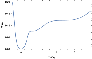
with , and . By integrating Eq. (22), we can get a generalized relation and the potential numerically as shown in Fig. 2. One notes that an inflection point exists in the scalar potential with the addition of the extra exponential term in the Kähler potential. When the pivotal scale leaves the horizon, or , so is small if and the effect of the exponential terms can be neglected. In this limit, the potential (31) reduces to the unmodified potential (24). In other word, the contribution from the extra exponential term can be ignored in the slow-roll regime.
We show four benchmark points in Table 1, where the -folding numbers are restricted to be . The parameters and affect the total -folding number. It is interesting to note that the -folding number spent around the inflection point is about , this is the reason why we can keep the remaining -folding number before the end of inflation to be . For the model I, we plot the potential for the inflaton field in Fig. 2. There is an inflection point at , where the slow-roll conditions are no longer satisfied. The evolutions of the inflaton and the slow-roll parameters and in terms of the number of -folds are shown in Fig. 3. The inflation ends at where the value of inflaton is for the model I. Near the inflection point at , there is a plateau in the evolution of inflaton as a function of the number of -folds , the slow-roll parameters are and , and the inflation lasts almost 15 -folds. This is important for the enhancement of the scalar power spectrum, since the power spectrum under the slow-roll approximation is given by
| (32) |
By varying the parameter , we can get an enhanced and then proper PBH abundance. However, this approximation in Eq. (32) fails to give us the accurate power spectrum near the inflection point. Thus, it is necessary to solve the Mukahanov-Sasaki equation numerically to obtain the accurate power spectrum.
| Model | |||||||||
|---|---|---|---|---|---|---|---|---|---|
| I | -0.480 | 46.79179 | 1.0032 | 2.463 | 0.7781 | 0.3936 | 0.9603 | 50.9 | |
| II | -0.480 | 46.7649 | 1.0031 | 2.466 | 0.7782 | 0.3935 | 0.9652 | 47.5 | |
| III | -0.470 | 43.62443 | 1.0020 | 2.485 | 0.8272 | 0.4043 | 0.9627 | 48.9 | |
| IV | -0.467 | 42.3915 | 1.0 | 2.50 | 0.8481 | 0.4087 | 0.9772 | 57.6 |
The numerical results for and at the pivotal scale are shown in Table 1, and they are consistent with the CMB constraints and [39, 115]. The mass and abundance of PBHs are sensitive to the parameters and . For a fixed , a smaller will give a more broad peak for and then produce PBHs with a larger peak mass. When is slightly bigger than , the -folding number increases rapidly and decreases to . The parameter is fixed by the amplitude of the power spectrum at the horizon crossing. The constraint on the amplitude of the power spectrum from Planck data is [39, 40].
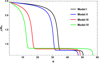
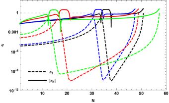
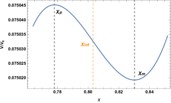
From Fig. 3, we see that the number of -folds near the inflection is about for the model I and II, whereas the number of -folds is about for the model III and for the model IV. When the inflaton climbs an upward step in the potential from its minimum to the maximum , the slow-roll parameter decreases and the power spectrum is enhanced. The climbing step is shown in the right panel of Fig. 2. Near the inflection point, the inflaton first decelerates and then accelerates when it rolls over the maximum point of the potential that gives the peak of the power spectrum. After the upward climbing, inflaton goes into the acceleration phase which decreases the power spectrum by the ratio [116]. As seen from Fig. 3, if increases more slowly after , then the inflaton stays near the inflection longer, and we get broader power spectrum. On the other hand, as shown in the right panel of Fig. 3, the minimum value of in the model IV is bigger, so its peak value of the power spectrum is expected to be smaller.
IV.1 Primordial curvature perturbations
Near the inflection point, the inflaton experiences a period of ultraslow-roll inflation and the amplitude of the primordial scalar power spectrum is enhanced. In order to obtain the power spectrum
| (33) |
for the primordial curvature perturbation , we numerically solve the Mukhanov-Sasaki equation [117, 118]
| (34) |
for the scalar mode , where the prime means derivative with respect to the conformal time , and can be expressed in terms of the Hubble slow-roll parameters as
| (35) |
with . In the limit , the mode function takes the solution
| (36) |
We plot the numerical results for the power spectrum in Fig. 4 and show the peak values of the power spectrum in Table 2. The black, red, blue, and green dashed lines correspond to the model I, II, III, and IV, respectively. Near the peak point , the power spectrum is enhanced to . The power spectrum in the models I and II has a sharp peak whereas the power spectrum in the models III and IV has a broad peak. The peak point in the model III and model IV are further away from the endpoint of inflaton than the other two models and the plateau in the potential of the inflaton in the models III and IV are more broader than the other two models.
| Model | |||||
|---|---|---|---|---|---|
| I | 0.023 | ||||
| II | 0.024 | ||||
| III | 0.036 | 0.018 | |||
| IV | 0.004 | 152 |
IV.2 PBH formation
The enhanced primordial curvature perturbations cause gravitational collapse in the overdense region at the horizon reentry during the radiation dominated era [28, 62, 33]. If the density fluctuation is larger than a centain threshold , the gravity can overcome the pressure and hence PBH forms. The critical threshold for PBH formation has a wide range, from 0.07 to 0.7 [130, 131, 132, 133, 134, 135]. In this paper, we take [136, 137, 138, 139]. Assuming the primordial perturbations obey Gaussian statistics, the fractional energy density of PBHs at their formation time is given by the Press-Schechter formalism [140]
| (37) |
where . The fractional energy density of PBHs with the mass to DM is [28, 33]
| (38) |
where kg is the solar mass, [141], [40]. The effective degrees of freedom at the time of PBH formation is in the radiation dominated era. The mass of PBHs is
| (39) |
Using the power spectrum obtained in Fig. 4, we calculate the mass and abundance of PBHs and display the results in Fig. 4 and Table 2. A wide mass range of PBH is realized in our model, and we show four benchmark points where the PBH masses are around , , and . The PBHs with masses around and can make up almost all DM and the peak abundances are . The PBH with the mass around only explains part of dark matter with . However, from Table 2, we see that the PBH with the mass around is hard to explain DM because of the significantly small value of .
IV.3 Scalar induced gravitational wave
Since the scalar perturbations and tensor perturbations are coupled at the second order, the large primordial curvature perturbation at small scales will induce second-order tensor perturbations. On CMB scale, the amplitude of tensor perturbation is much smaller than that of the scalar perturbation. The tensor-to-scalar ratio is constrained as (95% CL) [115]. Therefore, the second-order tensor perturbations induced by the enhanced scalar perturbations may be larger than primordial GWs. The perturbed metric in the Newtonian gauge is given by
| (40) |
In the following calculation, we will neglect the anisotropic stress, so . The equation of motion for the tensor mode, , sourced by the scalar perturbation , is
| (41) |
where the source term is given by
| (42) |
, is the polarization tensor. In the radiation domination, the Bardeen potential and the transfer function is
| (43) |
where , is the sound speed of the radiation background. The fluctuation is related to the primordial curvature perturbation as
| (44) |
The power spectrum of the tensor perturbation is defined as
| (45) |
After solving Eq. (41) with Green’s function method, the power spectrum can be written as [71, 72, 84]
| (46) |
and the fractional energy density of the induced GWs is
| (47) |
where the overline denotes the oscillation average, and . During the radiation era, the kernel function is [85, 71, 72, 84, 37]
| (48) |
where and .
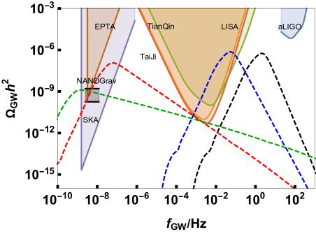
Converting the wave number to frequency with Hz/Mpc-1, the energy density of SIWGs against its frequency is plotted in Fig. 5. From Fig. 5, we see that the energy density of SIGWs illustrates some universal dependencies on the frequency [55, 142, 143]. The peak frequencies of these SIWGs are shown in Table 2. The SIWGs generated in the models III and IV have a wide peak. This broad band with frequencies Hz, comes from the broad enhanced power spectrum with the wavenumber Mpc-1. The produced PBH with the stellar mass can constitute part of DM in our universe. The SIWGs in the nanohertz band can be interpreted as the stochastic GW background observed by the recent 12.5-yr PTA data released by the NANOGrav [22, 93]. The broad band SIGWs can be tested by multiband GW observations. The SIWGs generated in the model II have a peak at the frequency Hz, which will be tested by the space-based GW detector, such as LISA, Taiji and TianQin. The SIWGs generated in the model I have a peak around the frequency 10 Hz which will be tested by the future ground-based GW observatory.
V Conclusion
We have investigated the formation of PBHs and SIGWs from the general no-scale supergravity inflationary model, inspired by the string model building. An inflection point is added by introducing an exponential term into Kähler potential. Thus, the amplitude of the primordial power spectrum is enhanced. To achieve the enhancement by the inflection point, the model parameters need to be fine-tuned by five decimal digits at most. The enhanced power spectra of primordial curvature perturbations can have both sharp and broad peaks. A wide mass range of PBH is realized in our model, and the frequencies of SIGWs are ranged form nanohertz to kilohertz. We have shown four benchmark points where the PBH masses are around , and and . The SIGWs accompanied with the formation of stellar mass PBH can interpret the stochastic GW background detected by NANOGrav. The PBHs with masses around and can make up almost all DM and the accompanied SIGWs will be testable by the upcoming space-based GW observatories. The observations of both PBHs and SIGWs can test our model and inflationary physics. The broad band SIGWs generated in this model can be tested by multiband GW observations.
Acknowledgements.
This work is supported in part by the National Natural Science Foundation of China under Grants No. 11875062, No. 11875136, and No. 11947302, the Major Program of the National Natural Science Foundation of China under Grant No. 11690021, the Key Research Program of Frontier Science, CAS. This work was also supported in part by the Natural Science Basic Research Plan in Shanxi Province of China under Grant No. 2020JQ-804, and by the Shanxi Provincial Education Department under Grant No. 20JK0685.References
- Abbott et al. [2016a] B. P. Abbott et al. (LIGO Scientific and Virgo Collaborations), Observation of gravitational waves from a binary black hole merger, Phys. Rev. Lett. 116, 061102 (2016a).
- Abbott et al. [2016b] B. P. Abbott et al. (LIGO Scientific and Virgo Collaborations), GW151226: observation of gravitational waves from a 22-solar-mass binary black hole coalescence, Phys. Rev. Lett. 116, 241103 (2016b).
- Abbott et al. [2017a] B. P. Abbott et al. (LIGO Scientific and Virgo Collaborations), GW170104: observation of a 50-solar-mass binary black hole coalescence at redshift 0.2, Phys. Rev. Lett. 118, 221101 (2017a); 121, 129901(E) (2018a) .
- Abbott et al. [2017b] B. P. Abbott et al. (LIGO Scientific and Virgo Collaborations), GW170814: a three-detector observation of gravitational waves from a binary black bole coalescence, Phys. Rev. Lett. 119, 141101 (2017b).
- Abbott et al. [2017c] B. P. Abbott et al. (LIGO Scientific and Virgo Collaborations), GW170817: observation of gravitational waves from a binary neutron star inspiral, Phys. Rev. Lett. 119, 161101 (2017c).
- Abbott et al. [2017d] B. P. Abbott et al. (LIGO Scientific and Virgo Collaborations), GW170608: observation of a 19-solar-mass binary black hole coalescence, Astrophys. J. Lett. 851, L35 (2017d).
- Abbott et al. [2019] B. P. Abbott et al. (LIGO Scientific and Virgo Collaborations), GWTC-1: a gravitational-wave transient catalog of compact binary mergers observed by LIGO and Virgo during the first and second observing runs, Phys. Rev. X 9, 031040 (2019).
- Abbott et al. [2020a] B. P. Abbott et al. (LIGO Scientific and Virgo Collaborations), GW190425: observation of a compact binary coalescence with total mass , Astrophys. J. Lett. 892, L3 (2020a).
- Abbott et al. [2020b] R. Abbott et al. (LIGO Scientific and Virgo Collaborations), GW190412: observation of a binary-black-hole coalescence with asymmetric masses, Phys. Rev. D 102, 043015 (2020b).
- Abbott et al. [2020c] R. Abbott et al. (LIGO Scientific and Virgo Collaborations), GW190814: gravitational waves from the coalescence of a 23 solar mass black hole with a 2.6 solar mass compact object, Astrophys. J. Lett. 896, L44 (2020c).
- Abbott et al. [2020d] R. Abbott et al. (LIGO Scientific and Virgo Collaborations), GW190521: a binary black hole merger with a total mass of , Phys. Rev. Lett. 125, 101102 (2020d).
- Abbott et al. [2021a] R. Abbott et al. (LIGO Scientific and Virgo Collaborations), GWTC-2: compact binary coalescences observed by LIGO and Virgo during the first half of the third observing run, Phys. Rev. X 11, 021053 (2021a).
- Abbott et al. [2021b] R. Abbott et al. (LIGO Scientific, VIRGO and KAGRA Collaborations), GWTC-3: compact binary coalescences observed by LIGO and Virgo during the second part of the third observing run, arXiv:2111.03606 .
- Garcia-Bellido et al. [1996] J. Garcia-Bellido, A. D. Linde, and D. Wands, Density perturbations and black hole formation in hybrid inflation, Phys. Rev. D 54, 6040 (1996).
- Leach and Liddle [2001] S. M. Leach and A. R. Liddle, Inflationary perturbations near horizon crossing, Phys. Rev. D 63, 043508 (2001).
- Bird et al. [2016] S. Bird, I. Cholis, J. B. Muñoz, Y. Ali-Haïmoud, M. Kamionkowski, E. D. Kovetz, A. Raccanelli, and A. G. Riess, Did LIGO detect dark matter?, Phys. Rev. Lett. 116, 201301 (2016).
- Sasaki et al. [2016] M. Sasaki, T. Suyama, T. Tanaka, and S. Yokoyama, Primordial black hole scenario for the gravitational-wave event GW150914, Phys. Rev. Lett. 117, 061101 (2016); 121, 059901(E) (2018) .
- De Luca et al. [2021a] V. De Luca, V. Desjacques, G. Franciolini, P. Pani, and A. Riotto, GW190521 mass gap event and the primordial black hole scenario, Phys. Rev. Lett. 126, 051101 (2021a).
- Scholtz and Unwin [2020] J. Scholtz and J. Unwin, What if Planet 9 is a primordial black hole?, Phys. Rev. Lett. 125, 051103 (2020).
- Takhistov et al. [2021] V. Takhistov, G. M. Fuller, and A. Kusenko, Test for the origin of solar mass black holes, Phys. Rev. Lett. 126, 071101 (2021).
- De Luca et al. [2021b] V. De Luca, G. Franciolini, and A. Riotto, NANOGrav data hints at primordial black holes as dark matter, Phys. Rev. Lett. 126, 041303 (2021b).
- Vaskonen and Veermäe [2021] V. Vaskonen and H. Veermäe, Did NANOGrav see a signal from primordial black hole formation?, Phys. Rev. Lett. 126, 051303 (2021).
- Ivanov et al. [1994] P. Ivanov, P. Naselsky, and I. Novikov, Inflation and primordial black holes as dark matter, Phys. Rev. D 50, 7173 (1994).
- Frampton et al. [2010] P. H. Frampton, M. Kawasaki, F. Takahashi, and T. T. Yanagida, Primordial black holes as all dark matter, J. Cosmol. Astropart. Phys. 04 (2010) 023.
- Belotsky et al. [2014] K. M. Belotsky, A. D. Dmitriev, E. A. Esipova, V. A. Gani, A. V. Grobov, M. Y. Khlopov, A. A. Kirillov, S. G. Rubin, and I. V. Svadkovsky, Signatures of primordial black hole dark matter, Mod. Phys. Lett. A 29, 1440005 (2014).
- Khlopov et al. [2005] M. Y. Khlopov, S. G. Rubin, and A. S. Sakharov, Primordial structure of massive black hole clusters, Astropart. Phys. 23, 265 (2005).
- Clesse and García-Bellido [2015] S. Clesse and J. García-Bellido, Massive primordial black holes from hybrid inflation as dark matter and the seeds of galaxies, Phys. Rev. D 92, 023524 (2015).
- Carr et al. [2016] B. Carr, F. Kuhnel, and M. Sandstad, Primordial black holes as dark matter, Phys. Rev. D 94, 083504 (2016).
- Inomata et al. [2017a] K. Inomata, M. Kawasaki, K. Mukaida, Y. Tada, and T. T. Yanagida, Inflationary primordial black holes as all dark matter, Phys. Rev. D 96, 043504 (2017a).
- García-Bellido [2017] J. García-Bellido, Massive primordial black holes as dark matter and their detection with gravitational waves, J. Phys. Conf. Ser. 840, 012032 (2017).
- Kovetz [2017] E. D. Kovetz, Probing primordial-black-hole dark matter with gravitational waves, Phys. Rev. Lett. 119, 131301 (2017).
- Carr and Kuhnel [2020] B. Carr and F. Kuhnel, Primordial black holes as dark matter: recent developments, Annu. Rev. Nucl. Part. Sci. 70, 355 (2020).
- Carr et al. [2020] B. Carr, K. Kohri, Y. Sendouda, and J. Yokoyama, Constraints on primordial black holes, arXiv:2002.12778 .
- Green and Kavanagh [2021] A. M. Green and B. J. Kavanagh, Primordial black holes as a dark matter candidate, J. Phys. G 48, 043001 (2021).
- Hawking [1971] S. Hawking, Gravitationally collapsed objects of very low mass, Mon. Not. R. Astron. Soc. 152, 75 (1971).
- Carr and Hawking [1974] B. J. Carr and S. W. Hawking, Black holes in the early Universe, Mon. Not. R. Astron. Soc. 168, 399 (1974).
- Lu et al. [2019] Y. Lu, Y. Gong, Z. Yi, and F. Zhang, Constraints on primordial curvature perturbations from primordial black hole dark matter and secondary gravitational waves, J. Cosmol. Astropart. Phys. 12, 031 (2019) .
- Sato-Polito et al. [2019] G. Sato-Polito, E. D. Kovetz, and M. Kamionkowski, Constraints on the primordial curvature power spectrum from primordial black holes, Phys. Rev. D 100, 063521 (2019).
- Akrami et al. [2020] Y. Akrami et al. (Planck Collaboration), Planck 2018 results. X. Constraints on inflation, Astron. Astrophys. 641, A10 (2020).
- Aghanim et al. [2020] N. Aghanim et al. (Planck Collaboration), Planck 2018 results. VI. Cosmological parameters, Astron. Astrophys. 641, A6 (2020); 652, C4(E) (2021).
- Kawasaki et al. [2016] M. Kawasaki, A. Kusenko, Y. Tada, and T. T. Yanagida, Primordial black holes as dark matter in supergravity inflation models, Phys. Rev. D 94, 083523 (2016).
- Di and Gong [2018] H. Di and Y. Gong, Primordial black holes and second order gravitational waves from ultra-slow-roll inflation, J. Cosmol. Astropart. Phys. 07 (2018) 007 .
- Garcia-Bellido et al. [2017] J. Garcia-Bellido, M. Peloso, and C. Unal, Gravitational wave signatures of inflationary models from primordial black hole dark matter, J. Cosmol. Astropart. Phys. 09 (2017) 013.
- Garcia-Bellido and Ruiz Morales [2017] J. Garcia-Bellido and E. Ruiz Morales, Primordial black holes from single field models of inflation, Phys. Dark Univ. 18, 47 (2017).
- Germani and Prokopec [2017] C. Germani and T. Prokopec, On primordial black holes from an inflection point, Phys. Dark Univ. 18, 6 (2017).
- Ezquiaga et al. [2018] J. M. Ezquiaga, J. Garcia-Bellido, and E. Ruiz Morales, Primordial black hole production in critical Higgs inflation, Phys. Lett. B 776, 345 (2018).
- Bezrukov et al. [2018] F. Bezrukov, M. Pauly, and J. Rubio, On the robustness of the primordial power spectrum in renormalized Higgs inflation, J. Cosmol. Astropart. Phys. 02 (2018) 040.
- Espinosa et al. [2018a] J. R. Espinosa, D. Racco, and A. Riotto, Cosmological signature of the standard model Higgs vacuum instability: primordial black holes as dark matter, Phys. Rev. Lett. 120, 121301 (2018a).
- Cicoli et al. [2018] M. Cicoli, V. A. Diaz, and F. G. Pedro, Primordial black holes from string inflation, J. Cosmol. Astropart. Phys. 06 (2018) 034.
- Gao and Guo [2018] T.-J. Gao and Z.-K. Guo, Primordial black hole production in inflationary models of supergravity with a single chiral superfield, Phys. Rev. D 98, 063526 (2018).
- Ballesteros et al. [2019] G. Ballesteros, J. Beltran Jimenez, and M. Pieroni, Black hole formation from a general quadratic action for inflationary primordial fluctuations, J. Cosmol. Astropart. Phys. 06 (2019) 016.
- Dalianis et al. [2019] I. Dalianis, A. Kehagias, and G. Tringas, Primordial black holes from -attractors, J. Cosmol. Astropart. Phys. 01 (2019) 037.
- Passaglia et al. [2020] S. Passaglia, W. Hu, and H. Motohashi, Primordial black holes as dark matter through Higgs field criticality, Phys. Rev. D 101, 123523 (2020).
- Bhaumik and Jain [2020] N. Bhaumik and R. K. Jain, Primordial black holes dark matter from inflection point models of inflation and the effects of reheating, J. Cosmol. Astropart. Phys. 01 (2020) 037.
- Xu et al. [2020] W.-T. Xu, J. Liu, T.-J. Gao, and Z.-K. Guo, Gravitational waves from double-inflection-point inflation, Phys. Rev. D 101, 023505 (2020).
- Braglia et al. [2020] M. Braglia, D. K. Hazra, F. Finelli, G. F. Smoot, L. Sriramkumar, and A. A. Starobinsky, Generating PBHs and small-scale GWs in two-field models of inflation, J. Cosmol. Astropart. Phys. 08 (2020) 001.
- Lin et al. [2020] J. Lin, Q. Gao, Y. Gong, Y. Lu, C. Zhang, and F. Zhang, Primordial black holes and secondary gravitational waves from and inflation, Phys. Rev. D 101, 103515 (2020).
- Yi et al. [2021a] Z. Yi, Y. Gong, B. Wang, and Z.-H. Zhu, Primordial black holes and secondary gravitational waves from the Higgs field, Phys. Rev. D 103, 063535 (2021a).
- Yi et al. [2021b] Z. Yi, Q. Gao, Y. Gong, and Z.-H. Zhu, Primordial black holes and scalar-induced secondary gravitational waves from inflationary models with a noncanonical kinetic term, Phys. Rev. D 103, 063534 (2021b).
- Gao et al. [2021] Q. Gao, Y. Gong, and Z. Yi, Primordial black holes and secondary gravitational waves from natural inflation, Nucl. Phys. B 969, 115480 (2021).
- Gao [2021] Q. Gao, Primordial black holes and secondary gravitational waves from chaotic inflation, Sci. China Phys. Mech. Astron. 64, 280411 (2021).
- Fu et al. [2019] C. Fu, P. Wu, and H. Yu, Primordial black holes from inflation with nonminimal derivative coupling, Phys. Rev. D 100, 063532 (2019).
- Fu et al. [2020] C. Fu, P. Wu, and H. Yu, Scalar induced gravitational waves in inflation with gravitationally enhanced friction, Phys. Rev. D 101, 023529 (2020).
- Dalianis et al. [2020] I. Dalianis, S. Karydas, and E. Papantonopoulos, Generalized non-minimal derivative coupling: application to inflation and primordial black hole production, J. Cosmol. Astropart. Phys. 06 (2020) 040.
- Ballesteros et al. [2020] G. Ballesteros, J. Rey, M. Taoso, and A. Urbano, Primordial black holes as dark matter and gravitational waves from single-field polynomial inflation, J. Cosmol. Astropart. Phys. 07 (2020) 025.
- Chen [2021] C.-Y. Chen, Threshold of primordial black hole formation in Eddington-inspired-Born–Infeld gravity, Int. J. Mod. Phys. D 30, 02 (2021).
- McDonough et al. [2020] E. McDonough, A. H. Guth, and D. I. Kaiser, Nonminimal couplings and the forgotten field of axion inflation, arXiv:2010.04179 .
- Ballesteros and Taoso [2018] G. Ballesteros and M. Taoso, Primordial black hole dark matter from single field inflation, Phys. Rev. D 97, 023501 (2018).
- Matarrese et al. [1998] S. Matarrese, S. Mollerach, and M. Bruni, Second order perturbations of the Einstein-de Sitter universe, Phys. Rev. D 58, 043504 (1998).
- Mollerach et al. [2004] S. Mollerach, D. Harari, and S. Matarrese, CMB polarization from secondary vector and tensor modes, Phys. Rev. D 69, 063002 (2004).
- Ananda et al. [2007] K. N. Ananda, C. Clarkson, and D. Wands, The Cosmological gravitational wave background from primordial density perturbations, Phys. Rev. D 75, 123518 (2007).
- Baumann et al. [2007] D. Baumann, P. J. Steinhardt, K. Takahashi, and K. Ichiki, Gravitational wave spectrum induced by primordial scalar perturbations, Phys. Rev. D 76, 084019 (2007).
- Saito and Yokoyama [2009] R. Saito and J. Yokoyama, Gravitational wave background as a probe of the primordial black hole abundance, Phys. Rev. Lett. 102, 161101 (2009); 107, 069901(E) (2011).
- Saito and Yokoyama [2010] R. Saito and J. Yokoyama, Gravitational-wave constraints on the abundance of primordial black holes, Prog. Theor. Phys. 123, 867 (2010); 126, 351(E) (2011).
- Bugaev and Klimai [2010] E. Bugaev and P. Klimai, Induced gravitational wave background and primordial black holes, Phys. Rev. D 81, 023517 (2010).
- Bugaev and Klimai [2011] E. Bugaev and P. Klimai, Constraints on the induced gravitational wave background from primordial black holes, Phys. Rev. D 83, 083521 (2011).
- Alabidi et al. [2012] L. Alabidi, K. Kohri, M. Sasaki, and Y. Sendouda, Observable spectra of induced gravitational waves from inflation, J. Cosmol. Astropart. Phys. 09 (2012) 017.
- Orlofsky et al. [2017] N. Orlofsky, A. Pierce, and J. D. Wells, Inflationary theory and pulsar timing investigations of primordial black holes and gravitational waves, Phys. Rev. D 95, 063518 (2017).
- Inomata et al. [2017b] K. Inomata, M. Kawasaki, K. Mukaida, Y. Tada, and T. T. Yanagida, Inflationary primordial black holes for the LIGO gravitational wave events and pulsar timing array experiments, Phys. Rev. D 95, 123510 (2017b).
- Cheng et al. [2018] S.-L. Cheng, W. Lee, and K.-W. Ng, Primordial black holes and associated gravitational waves in axion monodromy inflation, J. Cosmol. Astropart. Phys. 07 (2018) 001.
- Cai et al. [2019a] R.-G. Cai, S. Pi, and M. Sasaki, Gravitational waves induced by non-gaussian scalar perturbations, Phys. Rev. Lett. 122, 201101 (2019a).
- Bartolo et al. [2019a] N. Bartolo, V. De Luca, G. Franciolini, M. Peloso, D. Racco, and A. Riotto, Testing primordial black holes as dark matter with LISA, Phys. Rev. D 99, 103521 (2019a).
- Bartolo et al. [2019b] N. Bartolo, V. De Luca, G. Franciolini, A. Lewis, M. Peloso, and A. Riotto, Primordial black hole dark matter: LISA serendipity, Phys. Rev. Lett. 122, 211301 (2019b).
- Kohri and Terada [2018] K. Kohri and T. Terada, Semianalytic calculation of gravitational wave spectrum nonlinearly induced from primordial curvature perturbations, Phys. Rev. D 97, 123532 (2018).
- Espinosa et al. [2018b] J. R. Espinosa, D. Racco, and A. Riotto, A cosmological signature of the SM Higgs instability: gravitational waves, J. Cosmol. Astropart. Phys. 09 (2018) 012.
- Cai et al. [2019b] R.-G. Cai, S. Pi, S.-J. Wang, and X.-Y. Yang, Resonant multiple peaks in the induced gravitational waves, J. Cosmol. Astropart. Phys. 05 (2019) 013.
- Cai et al. [2020a] R.-G. Cai, Z.-K. Guo, J. Liu, L. Liu, and X.-Y. Yang, Primordial black holes and gravitational waves from parametric amplification of curvature perturbations, J. Cosmol. Astropart. Phys. 06 (2020) 013.
- Cai et al. [2019c] R.-G. Cai, S. Pi, S.-J. Wang, and X.-Y. Yang, Pulsar timing array constraints on the induced gravitational waves, J. Cosmol. Astropart. Phys. 10 (2019) 059.
- Domènech [2020] G. Domènech, Induced gravitational waves in a general cosmological background, Int. J. Mod. Phys. D 29, 2050028 (2020).
- Cai et al. [2021] R.-G. Cai, Y.-C. Ding, X.-Y. Yang, and Y.-F. Zhou, Constraints on a mixed model of dark matter particles and primordial black holes from the galactic 511 keV line, J. Cosmol. Astropart. Phys. 03 (2021) 057.
- Domènech et al. [2020] G. Domènech, S. Pi, and M. Sasaki, Induced gravitational waves as a probe of thermal history of the universe, J. Cosmol. Astropart. Phys. 08 (2020) 017.
- Arzoumanian et al. [2020] Z. Arzoumanian et al. (NANOGrav Collaboration), The NANOGrav 12.5 yr Data Set: Search for an isotropic stochastic gravitational-wave background, Astrophys. J. Lett. 905, L34 (2020).
- Kohri and Terada [2021] K. Kohri and T. Terada, Solar-mass primordial black holes explain NANOGrav hint of gravitational waves, Phys. Lett. B 813, 136040 (2021).
- Nakama et al. [2017] T. Nakama, J. Silk, and M. Kamionkowski, Stochastic gravitational waves associated with the formation of primordial black holes, Phys. Rev. D 95, 043511 (2017).
- Danzmann [1997] K. Danzmann, LISA: an ESA cornerstone mission for a gravitational wave observatory, Class. Quantum Grav. 14, 1399 (1997).
- Hu and Wu [2017] W.-R. Hu and Y.-L. Wu, The Taiji program in space for gravitational wave physics and the nature of gravity, Natl. Sci. Rev. 4, 685 (2017).
- Luo et al. [2016] J. Luo et al. (TianQin Collaboration), TianQin: a space-borne gravitational wave detector, Class. Quantum Grav. 33, 035010 (2016).
- Ellis et al. [2013a] J. Ellis, D. V. Nanopoulos, and K. A. Olive, Starobinsky-like inflationary models as avatars of no-scale supergravity, J. Cosmol. Astropart. Phys. 10(2013) 009.
- Ellis et al. [2013b] J. Ellis, D. V. Nanopoulos, and K. A. Olive, No-scale supergravity realization of the starobinsky model of inflation, Phys. Rev. Lett. 111, 111301 (2013b); 111, 129902(E) (2013b).
- Croon et al. [2013] D. Croon, J. Ellis, and N. E. Mavromatos, Wess-Zumino inflation in light of Planck, Phys. Lett. B 724, 165 (2013).
- Pi et al. [2018] S. Pi, Y.-l. Zhang, Q.-G. Huang, and M. Sasaki, Scalaron from -gravity as a heavy field, J. Cosmol. Astropart. Phys. 05 (2018) 042.
- Nanopoulos et al. [2020] D. V. Nanopoulos, V. C. Spanos, and I. D. Stamou, Primordial black holes from no-scale supergravity, Phys. Rev. D 102, 083536 (2020).
- Ellis et al. [2019] J. Ellis, D. V. Nanopoulos, K. A. Olive, and S. Verner, Unified no-scale attractors, J. Cosmol. Astropart. Phys. 09 (2019) 040.
- Ellis et al. [2020] J. Ellis, M. A. G. Garcia, N. Nagata, N. D. V., K. A. Olive, and S. Verner, Building models of inflation in no-scale supergravity, Int. J. Mod. Phys. D 29, 2030011 (2020).
- Stamou [2021] I. D. Stamou, Mechanisms of producing primordial black holes by breaking the symmetry, Phys. Rev. D 103, 083512 (2021).
- Cremmer et al. [1983] E. Cremmer, S. Ferrara, C. Kounnas, and D. V. Nanopoulos, Naturally vanishing cosmological constant in N=1 supergravity, Phys. Lett. B 133, 61 (1983).
- Lahanas and Nanopoulos [1987] A. B. Lahanas and D. V. Nanopoulos, The road to no scale supergravity, Phys. Rep. 145, 1 (1987).
- Witten [1985] E. Witten, Symmetry breaking patterns in superstring models, Nucl. Phys. B 258, 75 (1985).
- Li et al. [1997] T.-J. Li, J. L. Lopez, and D. V. Nanopoulos, Compactifications of M theory and their phenomenological consequences, Phys. Rev. D 56, 2602 (1997).
- Li [1998] T.-J. Li, Compactification and supersymmetry breaking in M theory, Phys. Rev. D 57, 7539 (1998).
- Ooguri and Vafa [2007] H. Ooguri and C. Vafa, On the geometry of the string landscape and the swampland, Nucl. Phys. B 766, 21 (2007).
- Obied et al. [2018] G. Obied, H. Ooguri, L. Spodyneiko, and C. Vafa, De Sitter space and the swampland, arXiv:1806.08362 [hep-th] .
- Gaillard et al. [1995] M. K. Gaillard, H. Murayama, and K. A. Olive, Preserving flat directions during inflation, Phys. Lett. B 355, 71 (1995).
- Diamandis et al. [1986] G. A. Diamandis, J. R. Ellis, A. B. Lahanas, and D. V. Nanopoulos, Vanishing scalar masses in no scale supergravity, Phys. Lett. B 173, 303 (1986).
- Ade et al. [2021] P. A. R. Ade et al. (BICEP and Keck Array Collaborations), Improved constraints on primordial gravitational waves using Planck, WMAP, and BICEP/Keck observations through the 2018 observing season, Phys. Rev. Lett. 127, 151301 (2021).
- Inomata et al. [2021] K. Inomata, E. McDonough, and W. Hu, Amplification of primordial perturbations from the rise or fall of the inflaton, arXiv:2110.14641 .
- Sasaki [1986] M. Sasaki, Large scale quantum fluctuations in the inflationary Universe, Prog. Theor. Phys. 76, 1036 (1986).
- Mukhanov [1988] V. F. Mukhanov, Quantum theory of gauge invariant cosmological perturbations, Sov. Phys. JETP 67, 1297 (1988).
- Fixsen et al. [1996] D. J. Fixsen, E. S. Cheng, J. M. Gales, J. C. Mather, R. A. Shafer, and E. L. Wright, The cosmic microwave background spectrum from the full COBE FIRAS data set, Astrophys. J. 473, 576 (1996).
- Carr et al. [2010] B. J. Carr, K. Kohri, Y. Sendouda, and J. Yokoyama, New cosmological constraints on primordial black holes, Phys. Rev. D 81, 104019 (2010).
- Graham et al. [2015] P. W. Graham, S. Rajendran, and J. Varela, Dark matter triggers of supernovae, Phys. Rev. D 92, 063007 (2015).
- Niikura et al. [2019] H. Niikura et al., Microlensing constraints on primordial black holes with Subaru/HSC Andromeda observations, Nat. Astron. 3, 524 (2019).
- Griest et al. [2013] K. Griest, A. M. Cieplak, and M. J. Lehner, New limits on primordial black hole dark matter from an analysis of Kepler source microlensing data, Phys. Rev. Lett. 111, 181302 (2013).
- Tisserand et al. [2007] P. Tisserand et al. (EROS-2 Collaboration), Limits on the macho content of the galactic halo from the EROS-2 survey of the magellanic clouds, Astron. Astrophys. 469, 387 (2007).
- Raidal et al. [2017] M. Raidal, V. Vaskonen, and H. Veermäe, Gravitational waves from primordial black hole mergers, J. Cosmol. Astropart. Phys. 09 (2017) 037.
- Ali-Haïmoud et al. [2017] Y. Ali-Haïmoud, E. D. Kovetz, and M. Kamionkowski, Merger rate of primordial black-hole binaries, Phys. Rev. D 96, 123523 (2017).
- Ali-Haïmoud and Kamionkowski [2017] Y. Ali-Haïmoud and M. Kamionkowski, Cosmic microwave background limits on accreting primordial black holes, Phys. Rev. D 95, 043534 (2017).
- Poulin et al. [2017] V. Poulin, P. D. Serpico, F. Calore, S. Clesse, and K. Kohri, CMB bounds on disk-accreting massive primordial black holes, Phys. Rev. D 96, 083524 (2017).
- Montero-Camacho et al. [2019] P. Montero-Camacho, X. Fang, G. Vasquez, M. Silva, and C. M. Hirata, Revisiting constraints on asteroid-mass primordial black holes as dark matter candidates, J. Cosmol. Astropart. Phys. 08 (2019) 031.
- Shibata and Sasaki [1999] M. Shibata and M. Sasaki, Black hole formation in the Friedmann universe: formulation and computation in numerical relativity, Phys. Rev. D 60, 084002 (1999).
- Polnarev and Musco [2007] A. G. Polnarev and I. Musco, Curvature profiles as initial conditions for primordial black hole formation, Class. Quantum Grav. 24, 1405 (2007).
- Musco et al. [2009] I. Musco, J. C. Miller, and A. G. Polnarev, Primordial black hole formation in the radiative era: investigation of the critical nature of the collapse, Class. Quantum Grav. 26, 235001 (2009).
- Musco and Miller [2013] I. Musco and J. C. Miller, Primordial black hole formation in the early universe: critical behaviour and self-similarity, Class. Quantum Grav. 30, 145009 (2013).
- Harada et al. [2013] T. Harada, C.-M. Yoo, and K. Kohri, Threshold of primordial black hole formation, Phys. Rev. D 88, 084051 (2013); 89, 029903(E) (2014).
- Germani and Musco [2019] C. Germani and I. Musco, Abundance of primordial black holes depends on the shape of the inflationary power spectrum, Phys. Rev. Lett. 122, 141302 (2019).
- Tada and Yokoyama [2019] Y. Tada and S. Yokoyama, Primordial black hole tower: dark matter, earth-mass, and LIGO black holes, Phys. Rev. D 100, 023537 (2019).
- Escrivà et al. [2020] A. Escrivà, C. Germani, and R. K. Sheth, Universal threshold for primordial black hole formation, Phys. Rev. D 101, 044022 (2020).
- Yoo et al. [2020] C.-M. Yoo, T. Harada, and H. Okawa, Threshold of primordial black hole formation in nonspherical collapse, Phys. Rev. D 102, 043526 (2020).
- Solbi and Karami [2021] M. Solbi and K. Karami, Primordial black holes and induced gravitational waves in -inflation, J. Cosmol. Astropart. Phys. 08 (2021) 056.
- Press and Schechter [1974] W. H. Press and P. Schechter, Formation of galaxies and clusters of galaxies by selfsimilar gravitational condensation, Astrophys. J. 187, 425 (1974).
- Carr [1975] B. J. Carr, The primordial black hole mass spectrum, Astrophys. J. 201, 1 (1975).
- Cai et al. [2020b] R.-G. Cai, S. Pi, and M. Sasaki, Universal infrared scaling of gravitational wave background spectra, Phys. Rev. D 102, 083528 (2020b).
- Yuan et al. [2020] C. Yuan, Z.-C. Chen, and Q.-G. Huang, Log-dependent slope of scalar induced gravitational waves in the infrared regions, Phys. Rev. D 101, 043019 (2020).
- Moore et al. [2015] C. J. Moore, R. H. Cole, and C. P. L. Berry, Gravitational-wave sensitivity curves, Class. Quant. Grav. 32, 015014 (2015).
- Ferdman et al. [2010] R. D. Ferdman et al., The european pulsar timing array: current efforts and a LEAP toward the future, Class. Quantum Grav. 27, 084014 (2010).
- Hobbs et al. [2010] G. Hobbs et al., The international pulsar timing array project: using pulsars as a gravitational wave detector, Class. Quantum Grav. 27, 084013 (2010).
- Hobbs [2013] G. Hobbs, The parkes pulsar timing array, Class. Quantum Grav. 30, 224007 (2013).
- McLaughlin [2013] M. A. McLaughlin, The north american nanohertz observatory for gravitational waves, Class. Quantum Grav. 30, 224008 (2013).
- Harry [2010] G. M. Harry (LIGO Scientific Collaboration), Advanced LIGO: the next generation of gravitational wave detectors, Class. Quantum Grav. 27, 084006 (2010).
- Aasi et al. [2015] J. Aasi et al. (LIGO Scientific Collaboration), Advanced LIGO, Class. Quantum Grav. 32, 074001 (2015).