Eigenvalue distribution of a high-dimensional

distance covariance matrix with application

Weiming Li, Qinwen Wang and Jianfeng Yao

Shanghai University of Finance and Economics,

Fudan University and The University of Hong Kong

Abstract:   We introduce a new random matrix model called distance covariance matrix in this paper, whose normalized trace is equivalent to the distance covariance. We first derive a deterministic limit for the eigenvalue distribution of the distance covariance matrix when the dimensions of the vectors and the sample size tend to infinity simultaneously. This limit is valid when the vectors are independent or weakly dependent through a finite-rank perturbation. It is also universal and independent of the details of the distributions of the vectors. Furthermore, the top eigenvalues of this distance covariance matrix are shown to obey an exact phase transition when the dependence of the vectors is of finite rank. This finding enables the construction of a new detector for such weak dependence where classical methods based on large sample covariance matrices or sample canonical correlations may fail in the considered high-dimensional framework.

Key words and phrases: Distance covariance; Distance covariance matrix; Eigenvalue distribution; Finite-rank perturbation; Nonlinear correlation; Spiked models.

1 Introduction

Székely et al. (2007) introduced the concept of distance covariance ${\mathcal{V}}(\bf x,\bf y)$ of two random vectors $({\bf x},{\bf y})\in\mathbb{R}^{p}\times\mathbb{R}^{q}$ as a measure of their dependence. It is defined through an appropriately weighted $L_{2}$-distance between the joint characteristic function $\phi_{\bf x,\bf y}(s,t)$ of $(\bf x,\bf y)$ and the product of their marginal characteristic functions $\phi_{\bf x}(s)\phi_{\bf y}(t)$, namely

$${\mathcal{V}}(\bf x,\bf y) =\left\{\frac{1}{c_{p}c_{q}}\int\!\!\!\int_{\mathbb{R}^{p}\times\mathbb{R}^{q}}\frac{|\phi_{\bf x,\bf y}(s,t)-\phi_{\bf x}(s)\phi_{\bf y}(t)|^{2}}{\|s\|^{1+p}\|t\|^{1+q}}dsdt\right\}^{\frac{1}{2}},$$ (1.1)

where the normalization constants are $c_{d}=\pi^{(1+d)/2}/\Gamma((1+d)/2)$ $(d=p,q)$. Clearly, ${{\mathcal{V}}(\bf x,\bf y)}=0$ if and only if $\bf x$ and $\bf y$ are independent.

For a collection of i.i.d. observations $({\bf x}_{1},{\bf y}_{1}),\ldots,({\bf x}_{n},{\bf y}_{n})$ from the population $({\bf x},{\bf y})$, Székely et al. (2007) proposed the sample distance covariance $\mathcal{V}_{n}({\bf x},{\bf y})$ as

$$\mathcal{V}_{n}({\bf x},{\bf y})=\left\{S_{1,n}+S_{2,n}-2S_{3,n}\right\}^{1/2},$$ (1.2)

where

$$S_{1,n} =\frac{1}{n^{2}}\sum_{k,\ell=1}^{n}\|{\bf x}_{k}-{\bf x}_{\ell}\|\|{\bf y}_{k}-{\bf y}_{\ell}\|,\quad$$

$$S_{2,n} =\frac{1}{n^{2}}\sum_{k,\ell=1}^{n}\|{\bf x}_{k}-{\bf x}_{\ell}\|\frac{1}{n^{2}}\sum_{k,\ell=1}^{n}\|{\bf y}_{k}-{\bf y}_{\ell}\|,$$

$$S_{3,n} =\frac{1}{n^{3}}\sum_{k,\ell,m=1}^{n}\|{\bf x}_{k}-{\bf x}_{\ell}\|\|{\bf y}_{k}-{\bf y}_{m}\|.$$

One remarkable result (Székely et al., 2007, Theorem 2) is that whenever ${\mathbb{E}}[\|{\bf x}\|+\|{\bf y}\|]<\infty$, ${\mathcal{V}}_{n}({\bf x},{\bf y})$ converges almost surely to $\mathcal{V}({\bf x},{\bf y})$ as $n\to\infty$. Based on this, a powerful statistic

$$T_{n}=n{\mathcal{V}}^{2}_{n}({\bf x},{\bf y})/S_{2,n}$$ (1.3)

was developed for testing the independence hypothesis,

$$H_{0}:{\bf x}~{}\text{is~{}independent~{}of~{}}{\bf y},$$ (1.4)

by establishing: (i) under $H_{0}$, $\displaystyle T_{n}\overset{\mathcal{D}}{\longrightarrow}Q$, a countable mixture of independent chi-squared distributions, and (ii) if ${\bf x}$ and ${\bf y}$ are dependent, $T_{n}\to\infty$ in probability. Such asymptotic theory for $T_{n}$ was established in the large sample asymptotics where the two dimensions $(p,q)$ are fixed while the sample size $n$ tends to infinity.

When the dimensions $(p,q)$ of the two vectors become large, Székely and Rizzo (2013) observed that the above test becomes invalid due to a non negligible bias of the squared sample distance covariance ${\mathcal{V}}_{n}^{2}({\bf x},{\bf y})$ and then proposed a bias-corrected version $\tilde{\mathcal{V}}_{n}^{2}({\bf x},{\bf y})$ as a substitution. By this correction, the sample distance correlation $\tilde{R}_{n}({\bf x},{\bf y})=\tilde{\mathcal{V}}_{n}({\bf x},{\bf y})/[\tilde{\mathcal{V}}_{n}({\bf x},{\bf x})\tilde{\mathcal{V}}_{n}({\bf y},{\bf y})]^{1/2}$ was employed for testing the independence hypothesis, whose null distribution was established in a specific asymptotic scheme where $n$ is kept fixed while $p$ and $q$ both grow to infinity. And this scheme is referred as fixed-$n$ asymptotic regime in the following. However, a recent paper Zhu et al. (2020) reported that even the test based on $\tilde{R}_{n}({\bf x},{\bf y})$ may loss the power for detecting nonlinear correlations when all the dimensions $(p,q,n)$ grow to infinity. In particular, they demonstrated that for high dimensional vectors, their squared sample distance covariance $\tilde{\mathcal{V}}_{n}^{2}({\bf x},{\bf y})$ is asymptotically equivalent to the summation of their squared component-wise (linear) cross sample covariances. This implies that distance covariance can only capture linear correlations in such high dimensional regimes.

To seek another possibility for detecting non-linear correlations between ${\bf x}$ and ${\bf y}$ when all the dimensions $(p,q,n)$ grow to infinity, we propose in this paper a new random matrix model, called distance covariance matrix (DCM). Specifically, denote two data matrices ${\mathbf{X}}=({\bf x}_{1},\ldots,{\bf x}_{n})$ and ${\mathbf{Y}}=({\bf y}_{1},\ldots,{\bf y}_{n})$, the DCM of ${\mathbf{X}}$ and ${\mathbf{Y}}$ is defined as

$${\mathbf{S}}_{xy}\triangleq{{\mathbf{P}}}_{n}{\mathbf{D}}_{x}{\bf P}_{n}{\mathbf{D}}_{y}{{\mathbf{P}}}_{n},$$ (1.5)

where

$${{\mathbf{D}}_{x}}\triangleq\frac{1}{p}{{\mathbf{X}}^{\prime}{\mathbf{X}}}+\frac{1}{pn}\sum_{i=1}^{n}||{\mathbf{x}}_{i}||^{2}{{\mathbf{I}}_{n}},\quad{{\mathbf{D}}_{y}}\triangleq\frac{1}{q}{{\mathbf{Y}}^{\prime}{\mathbf{Y}}+\frac{1}{qn}\sum_{i=1}^{n}||{\mathbf{y}}_{i}||^{2}{\mathbf{I}}_{n}},$$ (1.6)

and

$${\bf P}_{n}={\mathbf{I}}_{n}-\frac{1}{n}{\bf 1}_{n}{\bf 1}_{n}^{\prime}$$ (1.7)

is a projection matrix. The distance covariance matrix ${\mathbf{S}}_{xy}$ is closely connected to the distance covariance ${\mathcal{V}}({\bf x},{\bf y})$. As will be discussed in Section 2, a normalized trace of ${\mathbf{S}}_{xy}$ is asymptotically equivalent to the empirical distance covariance $\mathcal{V}_{n}({\bf x},{\bf y})$. Therefore, we believe that the spectrum of ${\mathbf{S}}_{xy}$ might contain the information indicating the non-linear dependence nature between ${\bf x}$ and ${\bf y}$. To this end, we investigate the first order asymptotic behaviors of the whole spectrum of the DCM ${\mathbf{S}}_{xy}$ under the two-sample Marčenko-Pastur asymptotic regime

$$(n,p,q)\to\infty,\quad(c_{n1},c_{n2}):=(p/n,q/n)\to(c_{1},c_{2})\in(0,\infty)^{2}.$$ (1.8)

Interestingly, we find that instead of the normalized trace of ${\mathbf{S}}_{xy}$, its largest eigenvalues have the ability to detect certain non-linear correlation between the two high dimensional random vectors ${\bf x}$ and ${\bf y}$.

The main contributions of the paper are three-folds. Our first result shows that the test statistic $T_{n}$ developed in Székely et al. (2007) for the independence hypothesis $H_{0}$ degenerates to the unit in the Marčenko-Pastur asymptotic regime, which extends a similar finding in Székely and Rizzo (2013) in their fixed-$n$ asymptotic regime. Therefore the statistic $T_{n}$ could not be applied any more for testing the independence hypothesis $H_{0}$ in the Marčenko-Pastur asymptotic regime (1.8).

As the second result of the paper, we derive a deterministic limiting distribution $F$ for the eigenvalue distribution of ${\mathbf{S}}_{xy}$. This means in particular that arbitrary eigenvalue statistic of the form $n^{-1}\sum_{i}g(\lambda_{i})$, where $(\lambda_{i})$ denotes the eigenvalues of ${\mathbf{S}}_{xy}$, with some smooth function $g$ converges to $\int g(x)dF(x)$. The limiting distribution $F$ is valid when the vectors are independent or weakly dependent corresponding to a finite-rank perturbation of the independence. An important property is that this limit is universal in the sense that it does not depend on the details of the respective distributions of the vectors.

Third, to further demonstrate the usefulness of such limiting eigenvalue distribution, we apply the theory to the problem of detection for certain deviation from the independence hypothesis by considering a family of finite-rank nonlinear dependence alternatives. We investigate both the global and local spectral behaviors of ${\mathbf{S}}_{xy}$. Globally, because the dependence is of finite rank, the limiting distribution of the eigenvalues remains the same as in the independence case, that is, the universal limit. However at a local scale, the largest eigenvalues of ${\mathbf{S}}_{xy}$ will converge to some limits outside the support of this universal limit as long as the strength of the dependence is beyond some critical value. Moreover, the locations of these outlying limits can be completely determined through the model parameters. Actually, these results under the finite-rank dependence is parallel with what is now known as Baik-Ben-Arous-Péché transition in random matrix theory, see Baik et al. (2005), Baik and Silverstein (2006) and Paul (2007). In this way, we conclude that the largest eigenvalues of ${\mathbf{S}}_{xy}$ can be used to detect such dependence structure. In addition, we propose an estimator for the rank of the dependence. This estimator is based on the ratios of adjacent largest eigenvalues of ${\mathbf{S}}_{xy}$. Its performance is assessed through simulation experiments.

Technically, our theoretical strategy for deriving the universal limit under independence is to derive a system of equations for the corresponding Stieltjes transform in the Gaussian case first. Indeed when the vectors ${\bf x}$ and ${\bf y}$ are Gaussian, the distance covariance matrix ${\mathbf{S}}_{xy}$ is orthogonally invariant; we can thus assume without loss of generality that the two population covariance matrices are diagonal, which greatly simplifies the analysis. In a second step, we obtain an accurate estimate for the difference between the Stieltjes transforms from Gaussian vectors and non-Gaussian ones by using a generalization of Lindeberg’s substitution method. This difference is indeed small enough so that the limiting distribution for the global spectrum of ${\mathbf{S}}_{xy}$ is actually universal, regardless of the underlying distributions of the vectors.

The rest of the paper is organized as follows. Section 2 details our model assumptions and the relation between the distance covariance matrix ${\mathbf{S}}_{xy}$ and the sample distance covariance ${\mathcal{V}}_{n}({\bf x},{\bf y})$. Section 3 establishes the limiting spectral distribution of ${\mathbf{S}}_{xy}$ under the Marčenko-Pastur asymptotic regime (1.8) when ${\bf x}$ and ${\bf y}$ are independent. Section 4 applies this theory to the detection of finite-rank nonlinear dependence between two high-dimensional vectors. All proofs of our technical results are gathered in an on-line supplementary file.

2 Distance covariance matrix

Let ${\mathbf{M}}_{p}$ be a $p\times p$ symmetric or Hermitian matrix with eigenvalues $(\lambda_{j})_{1\leq j\leq p}$. Its spectral distribution is the probability measure

$$F^{{\mathbf{M}}_{p}}=\frac{1}{p}\sum_{j=1}^{p}\delta_{\lambda_{j}},$$

where $\delta_{b}$ denotes the Dirac mass at $b$. For a probability measure $\mu$ on the real line (equipped with its Borel $\sigma$-algebra), its Stieltjes transform $s_{\mu}$ is a map from $\mathbb{C}^{+}$ onto itself,

$$s_{\mu}(z)=\int_{\mathbb{R}}\frac{1}{x-z}d\mu(x),\qquad z\in\mathbb{C}^{+},$$

where $\mathbb{C}^{+}\triangleq\{z\in\mathbb{C}:\Im(z)>0\}$.

Our asymptotic study of the spectrum of the DCM ${\mathbf{S}}_{xy}$ is developed under the following assumptions.

Assumption (a)

The dimensions $(n,p,q)$ tend to infinity as in (1.8).

Assumption (b)

The data matrices ${\mathbf{X}}=({\bf x}_{i})\in\mathbb{R}^{p\times n}$ and ${\mathbf{Y}}=({\mathbf{y}}_{i})\in\mathbb{R}^{q\times n}$ admit the following independent components model

$${\mathbf{X}}={\bf\Sigma}_{x}^{\frac{1}{2}}{\mathbf{W}}_{1}\quad\text{and}\quad{\mathbf{Y}}={\bf\Sigma}_{y}^{\frac{1}{2}}{\mathbf{W}}_{2},$$

where ${\bf\Sigma}_{x}\in\mathbb{R}^{p\times p}$ and ${\bf\Sigma}_{y}\in\mathbb{R}^{q\times q}$ denotes the population covariance matrices of ${\bf x}$ and ${\bf y}$, respectively, and $({\mathbf{W}}_{1}^{\prime},{\mathbf{W}}_{2}^{\prime})=(w_{ij})$ is an array of i.i.d. random variables satisfying

$${\mathbb{E}}(w_{11})=0,\quad{\mathbb{E}}(w_{11}^{2})=1,\quad{\mathbb{E}}|w_{11}|^{\gamma}<\infty,$$

for some $\gamma\geq 4$.

Assumption (c)

The spectral norms of $({\bf\Sigma}_{x},{\bf\Sigma}_{y})$ are uniformly bounded and their spectral distributions $(H_{xp},H_{yq})\triangleq(F^{{\bf\Sigma}_{x}},F^{{\bf\Sigma}_{y}})$ converge weakly to two probability distributions $(H_{x},H_{y})$, which are referred as population spectral distributions (PSD).

Our first result concerns the connection between our distance covariance matrix ${\mathbf{S}}_{xy}$ defined in (1.5) and the sample distance covariance ${\mathcal{V}}_{n}({\bf x},{\bf y})$ defined in (1.2).

Theorem 2.1.

Suppose that Assumptions (a)-(c) hold with some $\gamma>5$. Then we have

$$\mathcal{V}^{2}_{n}({\bf x},{\bf y})=\frac{1}{2n^{2}}\sqrt{\frac{pq}{\gamma_{x}\gamma_{y}}}{\text{\rm tr}}{\mathbf{S}}_{xy}+o_{p}(1).$$ (2.1)

Theorem 2.1 demonstrates that the squared sample distance covariance $\mathcal{V}^{2}_{n}({\bf x},{\bf y})$ is asymptotically equal to the normalized trace of the DCM ${\mathbf{S}}_{xy}$. As a first application of the DCM ${\mathbf{S}}_{xy}$, we use this approximation to establish below the degeneracy of the test statistic $T_{n}$ given in (1.3) for testing the independence hypothesis (1.4) under the Marčenko-Pastur asymptotic framework.

Theorem 2.2.

Suppose that Assumptions (a)-(c) hold with some $\gamma>5$. Then under the null hypothesis $H_{0}$, we have $\displaystyle T_{n}\to 1$ in probability.

A simple simulation experiment is conducted to exhibit the degeneracy of $T_{n}$ for two independent standard normal vectors. The dimension-to-sample size ratios are fixed to be $p/n=q/n=1/2$, the values of $p~{}(=q)$ range from $50$ to $400$, and the number of independent replications is $1000$. As shown in Table 2.1, with the growing of $p$, the empirical mean and standard deviation of $T_{n}$ converge to $1$ and $0$, respectively. Consequently, the test established in Székely et al. (2007) using the Chi-squares approximation will have a much inflated size tending to one when the dimensions are indeed large compared to the sample size.

Table 2.1: Empirical mean and standard deviation of the test statistic $T_{n}$ from 1000 independent replications with $p/n=q/n=1/2$ and $p\in\{50,100,200,400\}$. Independent standard normal vectors are used for ${\bf x}$ and ${\bf y}$.

$p=50$		$p=100$		$p=200$		$p=400$
mean	sd	mean	sd	mean	sd	mean	sd
1.0104	0.0075	1.0048	0.0036	1.0026	0.0018	1.0013	0.0009

3 Limiting spectral distribution of ${\mathbf{S}}_{xy}$ when ${\mathbf{x}}$ and ${\mathbf{y}}$ are independent

This section presents the first order convergence of the empirical spectral distribution $F^{{\mathbf{S}}_{xy}}$ of the DCM ${\mathbf{S}}_{xy}$ when ${\mathbf{x}}$ and ${\mathbf{y}}$ are independent.

Theorem 3.1.

Suppose that Assumptions (a)-(c) hold. Then, almost surely, the empirical spectral distribution $F^{{\mathbf{S}}_{xy}}$ converges weakly to a limiting spectral distribution (LSD) $F$ whose Stieltjes transform $s=s(z)$ is a solution to the following system of equations:

$$\begin{cases}\displaystyle s=\frac{wm-1}{z},\\ \displaystyle w=\int ts+\frac{ts}{1+tc_{1}^{-1}sm}dH_{x}(t),\\ \displaystyle m=\int t+\frac{t}{1+tc_{2}^{-1}w}dH_{y}(t),\end{cases}$$ (3.1)

where $w=w(z)$ and $m=m(z)$ are two auxiliary analytic functions. The solution is also unique on the set

$$\{s(z):s(z)\in\mathbb{C}^{+},w(z)\in\mathbb{C}^{+},m(z)\in\mathbb{C}^{-},z\in\mathbb{C}^{+}\}.$$ (3.2)

Remark 3.1.

The two auxiliary functions $w(z)$ and $m(z)$ are respectively the limits of $w_{n}(z)$ and $m_{n}(z)$ defined in (B.16) of the supplementary document. Their construction accounts for the signs of their imaginary parts as in (3.2).

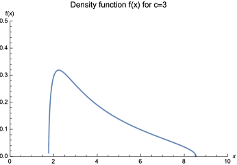
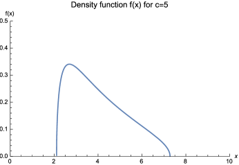
Figure 3.1: Density curves of LSDs for $c=3$ (left) and $c=5$ (right). The PSDs are $H_{x}=H_{y}=\delta_{1}$.

Next, we provide an illustration of how to calculate the LSD $F$ through the system of equations (3.1). Considering the case where the two populations ${\bf x}$ and ${\mathbf{y}}$ are of the same dimension and both have the identity covariance matrices, we thus have

$$c_{1}=c_{2}=c\quad\text{and}\quad H_{x}=H_{y}=\delta_{1}.$$ (3.3)

For this case, a closed-form solution to the system (3.1) does exist, that is, the Stieltjes transform $s=s(z)$ of the LSD $F$ satisfies the following

$$c^{2}-s+2cs-4c^{2}s+s^{2}+c^{2}sz-2s^{2}z+2cs^{2}z+s^{3}z-s^{3}z^{2}=0.$$ (3.4)

Substituting $z=x+{\rm i}v$ and $s=s_{u}+{\rm i}s_{v}$ into (3.4) and then letting $v\downarrow 0$, we get the following system of equations by separating the real and imaginary parts on the left hand side of (3.4),

$$\left\{\begin{array}[]{l}\displaystyle s_{v}^{2}=\frac{c^{2}-s_{u}+2cs_{u}-4c^{2}s_{u}+c^{2}xs_{u}+s_{u}^{2}-2xs_{u}^{2}+2cxs_{u}^{2}+xs_{u}^{3}-x^{2}s_{u}^{3}}{1-2x+2cx+3xs_{u}-3x^{2}s_{u}},\vspace{1ex}\\ \displaystyle s_{v}^{2}=\frac{1-2c+4c^{2}-c^{2}x-2s_{u}+4xs_{u}-4cxs_{u}-3xs_{u}^{2}+3x^{2}s_{u}^{2}}{-x+x^{2}}.\end{array}\right.$$ (3.7)

Cancelling the variable $s_{u}$ from (3.7), one may get three solutions for $s_{v}^{2}$ as a function of $x$. These three functions indeed have closed forms, but are lengthy and we omit their explicit expressions here. Then for each real value of $x$, only one solution of $s_{v}^{2}$ is real and nonnegative, which corresponds to the density function $f(x)$ of the LSD $F$, i.e. $f(x)=\sqrt{s_{v}^{2}}/\pi$. Using this approach, we plot in the following Figure 3.1 two LSDs for such particular setting (3.3) corresponding to $c=3$ and $c=5$. However, generally when there is no closed-form solution for (3.1), we rely on numerical approximations for the limiting Stieltjes transform $s(z)$ and the underlying limiting density function. These methods are used in the illustration below and also in the simulation experiments in Section 4.

Some numerical illustrations of Theorem 3.1 are conducted under two models:

• Model 1: $H_{x}=H_{y}=\delta_{1}$, $c_{1}=c_{2}=1$, $z_{11}\sim N(0,1)$;

• Model 2: $H_{x}=0.5\delta_{0.5}+0.5\delta_{1}$, $H_{y}=0.5\delta_{0.25}+0.5\delta_{0.75}$, $c_{1}=2,c_{2}=1$, and $z_{11}\sim(\chi^{2}_{v}-v)/\sqrt{2v}$, a standardized chi-squared distribution with degree of freedom $v=2$.

The PSDs in the first model are simple point masses and the system (3.1) defining the LSD simplifies to a single equation $(z^{2}-z)s^{3}-s^{2}+(3-z)s-1=0$ (letting $c=1$ in (3.4)). The second model is a bit more elaborated where the PSDs are mixtures of two point masses and the innovations $z_{ij}$’s are Chi-square distributed with heavy tails.

To exhibit the LSDs defined by Models 1 and 2, we simply approximate their density functions by $\hat{f}(x)=\Im s(x+{\rm i}/10^{4})/\pi,x\in\mathbb{R}.$ This approximation is justified by the inversion formula of Stieltjes transforms, i.e. $f(x)=\lim_{\varepsilon\to 0^{+}}\Im s(x+{\rm i}\varepsilon)/\pi,$ provided the limit exists, see Theorem B.10 in Bai and Silverstein (2010). Obviously, our approximation takes $\varepsilon=10^{-4}$ which is small enough for the illustration here. Next, for any given $z=x+{\rm i}/10^{4}$, we numerically solve the system of equations in (3.1) and select the unique solution $(s(z),w(z),m(z))$ satisfying (3.2), which is done automatically in Mathematica software. Finally, taking the imaginary part of $s(z)/\pi$ gives $\hat{f}(x)$.

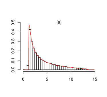
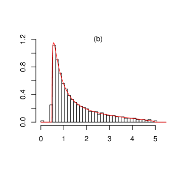
Figure 3.2: Histogram of eigenvalues of the matrix ${\mathbf{S}}_{xy}$ under Model 1 (left panel) with dimensions $p=q=n=500$ and Model 2 (right panel) with dimensions $p=2q=2n=800$. The fitted curves (red colored) are the corresponding densities of the LSDs.

In this simulation experiment, the empirical PSDs are chosen as their limiting ones and the dimensions are $(p,q,n)=(500,500,500)$ for Model 1 and $(p,q,n)=(800,400,400)$ for Model 2. All eigenvalues are collected from 100 independent replications. The averaged histograms of the eigenvalues of ${\mathbf{S}}_{xy}$ from those replications are depicted in Figure 3.2. It shows that these empirical distributions match well their limiting density curves predicted in Theorem 3.1.

4 Application to the detection of dependence between two high dimensional vectors

Theorem 3.1 determines a universal limit for the bulk spectrum of the DCM when the two sets of samples are independent. A natural question arises: how this bulk limit will evolve when they become dependent? Apparently if their inherent dependence is very strong, the spectral limit of the DCM will be totally different from the universal limit in Theorem 3.1. Here we choose to study a special type of weak dependence which is finite rank dependence. Such concept is parallel to the idea of finite-rank perturbation or spiked population models in high-dimensional statistics which are widely studied in connection with high-dimensional PCA, factor modeling and the signal detection problem (Johnstone and Paul, 2018). A striking finding from the work here is that such finite-rank nonlinear dependence can be detected using the largest eigenvalues of the DCM while existing methods based on sample covariance, sample correlation or sample canonical correlations will fail.

4.1 Extreme eigenvalues of distance covariance matrix under finite-rank dependence

Precisely, we consider two dependent populations ${\mathbf{x}}\in\mathbb{R}^{p}$ and ${\mathbf{z}}\in\mathbb{R}^{q}$ defined as follows:

• For a fixed $m\in\mathbb{N}$, let $({\mathbf{u}}_{k})_{1\leq k\leq m}$ and $({\mathbf{v}}_{k})_{1\leq k\leq m}$ be two independent sequences of i.i.d. vectors distributed uniformly on the unit spheres in $\mathbb{R}^{q}$ and $\mathbb{R}^{p}$, respectively.

• Given the sequences $({\mathbf{u}}_{k})$ and $({\mathbf{v}}_{k})$, the population ${\mathbf{z}}$ is defined as

  $${\mathbf{z}}=\varepsilon\left(\sum_{k=1}^{m}\theta_{k}{\mathbf{u}}_{k}{\mathbf{v}}^{\prime}_{k}\right){\mathbf{x}}+{\mathbf{y}},$$ (4.1)

where

• ${\mathbf{x}}\in\mathbb{R}^{p}$ and ${\mathbf{y}}\in\mathbb{R}^{q}$ satisfy Assumptions (b) and (c);

• $\varepsilon$ is a standardized random variable with finite fourth moment.

• $0<\theta_{m}<\cdots<\theta_{1}<\infty$ are $m$ constants reflecting the strengths of dependence between ${\mathbf{x}}$ and ${\mathbf{z}}$.

Remark 4.1.

The pair of random vectors $({\mathbf{x}},{\mathbf{z}})$ in (4.1) are nonlinearly dependent, that is, they are uncorrelated but dependent. To see this, consider a particular case such that $\varepsilon$ is a random sign taking values $1$ or $-1$ with equal probability. Then it is easy to see that the random sign $\varepsilon$ put on the vector ${\bf x}$ implies the uncorrelation between the vectors. To establish their dependence, simple algebra shows that

$${\mathbb{E}}\big{(}\|{\mathbf{x}}\|^{2}\big{)}{\mathbb{E}}\big{(}\|{\mathbf{z}}\|^{2}\big{)} =\frac{1}{p}\|\theta\|^{2}{\mathbb{E}}^{2}\big{(}\|{\mathbf{x}}\|^{2}\big{)}+{\mathbb{E}}\|{\mathbf{x}}\|^{2}{\mathbb{E}}\|{\mathbf{y}}\|^{2},$$

$${\mathbb{E}}\big{(}\|{\mathbf{x}}\|^{2}\|{\mathbf{z}}\|^{2}\big{)} =\frac{1}{p}\|\theta\|^{2}{\mathbb{E}}\|{\mathbf{x}}\|^{4}+{\mathbb{E}}\|{\mathbf{x}}\|^{2}{\mathbb{E}}\|{\mathbf{y}}\|^{2}.$$

Here, $\|\theta\|^{2}=\theta_{1}^{2}+\cdots+\theta_{m}^{2}$. Unless ${\mathbf{x}}$ is a constant vector, ${\mathbb{E}}\|{\mathbf{x}}\|^{4}>{\mathbb{E}}^{2}\big{(}\|{\mathbf{x}}\|^{2}\big{)}$ and thus the vectors ${\mathbf{x}}$ and ${\mathbf{z}}$ are dependent.

Suppose we have an i.i.d.  sample $({\mathbf{x}}_{1},{\mathbf{z}}_{1}),\ldots,({\mathbf{x}}_{n},{\mathbf{z}}_{n})$ from the population $({\mathbf{x}},{\mathbf{z}})\in\mathbb{R}^{p}\times\mathbb{R}^{q}$ defined in (4.1). Denote by ${\mathbf{X}}=({\mathbf{x}}_{1},\ldots,{\mathbf{x}}_{n})$ and ${\mathbf{Z}}=({\mathbf{z}}_{1},\ldots,{\mathbf{z}}_{n})$ the two data matrices with sizes $p\times n$ and $q\times n$, respectively. Similar to the matrices in (1.6) we define two matrices ${\mathbf{D}}_{x}$ and ${\mathbf{D}}_{z}$ as

$${\mathbf{D}}_{x}=\frac{1}{p}{{\mathbf{X}}^{\prime}{\mathbf{X}}}+\kappa_{x}{\bf I}_{n}\quad\text{and}\quad{\mathbf{D}}_{z}=\frac{1}{q}{{\mathbf{Z}}^{\prime}{\mathbf{Z}}}+\kappa_{z}{\bf I}_{n},$$

where

$$\kappa_{x}\triangleq(pn)^{-1}\sum_{i=1}^{n}||{\bf x}_{i}||^{2}\quad\text{and}\quad\kappa_{z}\triangleq(qn)^{-1}\sum_{i=1}^{n}||{\mathbf{z}}_{i}||^{2}.$$

The corresponding DCM is written as

$${\mathbf{S}}_{xz}\triangleq{\mathbf{P}}_{n}{\mathbf{D}}_{x}{\mathbf{P}}_{n}{\mathbf{D}}_{z}{\mathbf{P}}_{n}.$$

We will study the spectral properties of ${\mathbf{S}}_{xz}$ for the dependent pair $({\mathbf{x}},{\mathbf{z}})$ defined in (4.1). First of all, because the rank of perturbation is finite, it is shown that the limiting spectral distribution of ${\mathbf{S}}_{xz}$ remains the same as if the two populations are independent.

Theorem 4.1.

Suppose that Assumptions (a)-(c) hold for model (4.1). The limiting spectral distribution of ${\mathbf{S}}_{xz}$ is given by the same $F$ defined in Theorem 3.1.

According to Theorem 4.1, the global behavior of the eigenvalues of the DCM ${\mathbf{S}}_{xz}$ will not be useful for distinguishing such weak dependence from the independence scenario. In the following, we turn to study the top eigenvalues of the ${\mathbf{S}}_{xz}$ and show that the weak dependence structure is encoded in these top eigenvalues. Detection of such weak dependence thus becomes possible using these top eigenvalues. Before that, we introduce some notations that will be used for stating our result. We denote

$$\lambda_{+}=\limsup_{n\to\infty}\|{\mathbf{S}}_{xy}\|,$$

which is finite. On $(\lambda_{+},\infty)$, define the function

$$g(\lambda)=-\int tdH_{x}(t)\int\frac{w(\lambda)}{c_{2}+tw(\lambda)}dH_{y}(t),\quad\lambda>\lambda_{+},$$ (4.2)

where $w(z)$ is given in (3.1). It’s easy to verify that $g(\lambda)>0$, $g^{\prime}(\lambda)<0$ and $\lim_{\lambda\to+\infty}g(\lambda)=0.$ Next, define

$$\theta_{0}:=\lim_{\lambda\,\downarrow\,\lambda_{+}}[g(\lambda)]^{-\frac{1}{2}}.$$ (4.3)

Therefore $g$ is a one-to-one, strictly decreasing and nonnegative function from $(\lambda_{+},\infty)$ to $(1/\theta_{0}^{2},0)$.

Theorem 4.2.

Suppose that Assumptions (a)-(c) hold for model (4.1) and for some $k\in\{1,\ldots,m\}$, $\theta_{k}>\theta_{0}$. Then the $k$-th largest eigenvalue $\lambda_{n,k}$ of the DCM ${\mathbf{S}}_{xz}$ converges almost surely to a limit

$$\lambda_{k}=g^{-1}\big{(}1/{\theta_{k}^{2}}\big{)}>\lambda_{+},$$ (4.4)

where $g^{-1}$ denotes the functional inverse of $g$.

Remark 4.2.

Generally, the function $g$ as well as the critical value $\theta_{0}$ have no analytic formulas and both can be found numerically for any given model settings. However, in certain particular case, for example the setting considered in (3.3), the function $g(\lambda)$ given in (4.2) is a solution to

$$cg^{3}(\lambda)+(1+4c)g^{2}(\lambda)+g(\lambda)(3+4c-c\lambda)+2=0.$$ (4.5)

In fact there are three solutions to (4.5) which all have explicit but lengthy expressions. One may choose the one that monotonically decreases to zero as $\lambda$ tends to infinity, which is our target function $g(\lambda)$. Then the critical value $\theta_{0}=[g(\lambda_{+})]^{-1/2}$ can be obtained accordingly. Note that the right edge $\lambda_{+}$ of the LSD $F$ can be theoretically derived by setting the density function $f(x)$ to be zero. As an illustration, we exhibit the relation between the value $\theta_{0}$ and the ratio $c$ for the case (3.3) in Figure 4.1.

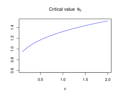
Figure 4.1: Critical value $\theta_{0}$ for $c_{1}=c_{2}=c$ and $H_{x}=H_{y}=\delta_{1}$.

The limit $\lambda_{k}$ in (4.4) is outside the support of the LSD $F$. A technical point here is that Theorem 4.2 does not tell what happens to $\lambda_{n,k}$ if $\theta_{k}\leq\theta_{0}$. By assuming the convergence of the largest eigenvalue of the base component ${\mathbf{S}}_{xy}$ to the right edge point of the LSD, we can establish the following exact phase transition for the top eigenvalues $\lambda_{n,k}~{}(1\leq k\leq m)$.

Corollary 4.1.

In addition to Assumptions (a)-(c) for model (4.1), suppose that the largest eigenvalue of the DCM ${\mathbf{S}}_{xy}$ converges to $\lambda_{+}$, which is the right edge point of the LSD $F$. Then for $k=1,\ldots,m$,

$$\lambda_{n,k}\xrightarrow{a.s.}\begin{cases}\lambda_{k}&\text{if}~{}\theta_{k}>\theta_{0},\\ \lambda_{+}&\text{if}\ \theta_{k}\leq\theta_{0},\end{cases}$$

where $\theta_{0}$ and $\lambda_{k}$ are given in (4.3) and (4.4), respectively.

Corollary 4.1 follows directly from the proof of Theorem 4.2 and the classic interlacing theorem. It implies the value $\theta_{0}$ is the exact critical value for the phase transition of the top eigenvalues of the DCM ${\mathbf{S}}_{xz}$. Note that the convergence of the largest eigenvalue of the (null) DCM ${\mathbf{S}}_{xy}$ to $\lambda_{+}$ is needed and assumed here to ensure the convergence of those sub-critical spike eigenvalues, i.e. $\theta_{k}\leq\theta_{0}$, to the same right edge point $\lambda_{+}$. On the other hand, very likely this largest eigenvalue does converge. However, proof for such convergence of the largest eigenvalue would be lengthy and technical, and we leave it for future investigation.

4.2 Monte Carlo experiments

This section examines finite sample properties of the outlier eigenvalues of ${\mathbf{S}}_{xz}$. To simplify the exposition, we consider only the rank-one situation ($m=1$) in this section. Higher dependence ranks with $m>1$ will be discussed in Section 4.3. Three models are taken into consideration under normal populations:
Model 4: $H_{x}=H_{y}=\delta_{1},\ c_{1}=c_{2}=2;\\$ Model 5: $H_{x}=H_{y}=\delta_{1},\ c_{1}=0.1,\ c_{2}=0.2;\\$ Model 6: $H_{x}=0.5\delta_{0.5}+0.5\delta_{1},\ H_{y}=0.5\delta_{1}+0.5\delta_{1.5},\ c_{1}=1,c_{2}=2.\\$ Models 4 and 5 are both standard normal population, with different dimension-to-sample size ratios. Model 6 is more general by employing two discrete PSDs. All statistics are calculated using 1000 independent replications.

We begin with the convergence of the largest eigenvalue of ${\mathbf{S}}_{xz}$ under Model 4. Theoretically, the largest eigenvalue will become an outlier when $\theta>{\ \theta_{0}=}1.52$ (see Figure 4.1 for the critical value). The parameter $\theta$ is thus set to be $\theta=0,1,2,3$. The sample size $n$ ranges from 100 to 1600. Empirical mean and standard deviation of the largest eigenvalue are collected in Table 4.1. It shows that, for $\theta=0$ and 1 (second to fifth columns), the largest eigenvalue increases with decreasing standard error as $n$ grows and is close to $\lambda_{+}=9.95$, the right edge point of $F$. When $\theta={2}$ and 3 (last four columns), the largest eigenvalue converges to its theoretical limit $\lambda=10.6875$ for $\theta=2$ and $\lambda=15.0123$ for $\theta=3$. These results fully coincide with the conclusions of Theorem 4.2.

Table 4.1: Empirical mean and standard deviation of the largest eigenvalue under Model 4. The setting is $c_{n1}=c_{n2}=2$ with varying $n$ and 1000 independent replications. The right edge point of the LSD is $\lambda_{+}=9.95$.

	$\theta=0$		$\theta=1$		$(\theta,\lambda)=(2,10.6875)$		$(\theta,\lambda)=(3,15.0123)$
$n$	mean	sd	mean	sd	mean	sd	mean	sd
$100$	9.5732	0.3126	9.6443	0.3419	10.7285	0.7055	15.1056	1.5770
$200$	9.7247	0.1972	9.7486	0.2013	10.7219	0.5048	15.0821	1.1099
$400$	9.8094	0.1302	9.8209	0.1239	10.7114	0.3500	15.0446	0.7458
$800$	9.8587	0.0769	9.8729	0.0796	10.7079	0.2531	14.9985	0.5505
$1600$	9.8950	0.0479	9.8966	0.0502	10.6985	0.1745	15.0249	0.3794

Next we study the evolution of the outlier limit $\lambda(\theta)$ in function of the dependence strength $\theta$. Models 5 and 6 are considered with the dimensions fixed at $(p,q,n)=(200,400,2000)$ for Model 5 and at $(p,q,n)=(800,800,400)$ for Model 6. The parameter $\theta$ ranges from 0 to 2.5 for Model 5 and from 0 to 5 for Model 6. Figure 4.2 displays the average of the largest eigenvalue with $\pm 1$ standard deviations (vertical bars). The dashed red lines mark the right boundary of $F$ and the solid red lines are the theoretical curves of $\lambda=\lambda(\theta)$. Both the two graphs in Figure 4.2 exhibit a common trend that the largest eigenvalue will depart from the bulk when $\theta$ crosses a critical value and goes up with increasing standard deviation.

abcdefg

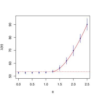
Figure 4.2: The average of the largest eigenvalue under Model 5 (left panel) and Model 6 (right panel) from 1000 independent replications with $\pm 1$ standard deviations (blue bars). The solid red line is the limiting curve of the function $\lambda(\theta)$ and the dashed red line represents the right boundary of LSD’s support.

Lastly, we compare the performance of using the largest eigenvalues of our DCM model with high-dimensional CCA (Yang and Pan, 2015; Bao et al., 2019) for detecting dependence between two groups of random samples. As is well known, a direct application of CCA often fails for the detection when the two sample sets are dependent but uncorrelated. It is thus suggested in Yang and Pan (2015) to transform the data in a suitable way before applying CCA if one has some prior knowledge of the dependence structure. We refer to this variant of CCA as TCCA in the following.

Model 5 is employed in this experiment. The parameter settings are $\theta=2,4,10$ and $(p,q,n)=(100,200,1000)$. For the TCCA method, we use the exponential function $f(x)=e^{x}$ to transform each coordinate of the sample vectors and then conduct the CCA procedure. In this way, the two sets of transformed data are indeed linearly correlated.

Histograms of the bulk eigenvalues and the largest eigenvalue are plotted in Figure 4.3. On the left panel, the eigenvalues are from the DCM ${\mathbf{S}}_{xz}$. One may see that the empirical SD of the bulk eigenvalues (black strips) is perfectly predicted by its LSD density curve (red lines). Moreover, the largest eigenvalues (blue strips) are centered at $\lambda=69.83,187.5$, and $1041.5$ (blue lines) for $\theta=2,4$ and $10$, respectively, which are clearly separated from the bulks. Similar statistics from CCA are shown on the middle panel. It demonstrates that the largest eigenvalues for $\theta=2,4,10$ are all centered at $\lambda=0.49$ which is smaller than the right edge point $\lambda_{+}=0.5$ of the LSD. Results from TCCA are plotted on the right panel, where the largest eigenvalues are centered at $\lambda=0.49,0.50,0.52$ for $\theta=2,4,10$, respectively. On the other hand, Figure 4.4 reports the sequences of sample ratios $\{\lambda_{n,i+1}/\lambda_{n,i}\}$ with $\pm 2$ standard deviations. For $\theta=2,4,10$, the first ratio $\{\lambda_{n,2}/\lambda_{n,1}\}$ from the DCM model is well separated from the rest ones while those from the CCA and TCCA models have no clear separation. Therefore, the non-linear correlation between ${\mathbf{x}}$ and ${\mathbf{z}}$ can be entirely captured by the DCM model while CCA and TCCA will both fail to distinguish it efficiently. We note that for the TCCA method, it indeed has some potential for the detection as one may observe that, on average, the largest eigenvalue from TCCA can surpass the right edge limit $0.5$ of the LSD as the parameter $\theta$ increases. However its power is weak compared with our proposed method for the studied cases. Some other transforms are also tested under the same settings, such as polynomial functions, Box-Cox transforms, and trigonometric functions. Their performance is either comparable with or less superior to the exponential function.

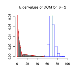
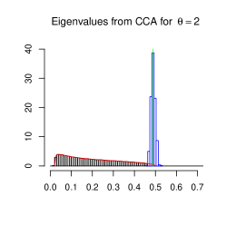
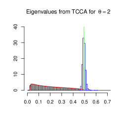
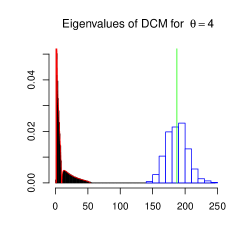
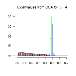
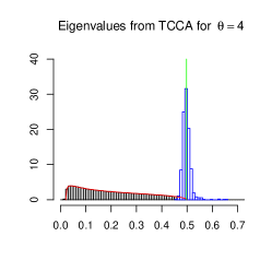
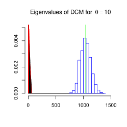
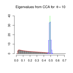
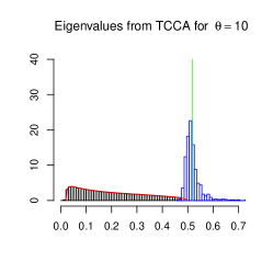
Figure 4.3: Histograms of bulk eigenvalues (black strips) and the largest eigenvalue (blue strips) from 1000 independent replications under Model 5 with $\theta=2,4,$ and $10$. The red curves are LSD densities and the green vertical lines locate at the averages of the largest eigenvalues. Plots on the left panel are based on the DCM ${\mathbf{S}}_{xz}$ while those on the middle and left panels are based on CCA and TCCA, respectively. The dimensions are $(p,q,n)=(100,200,1000)$.

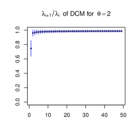
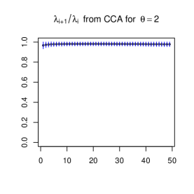
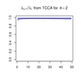
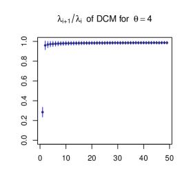
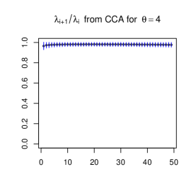
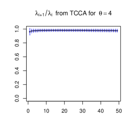
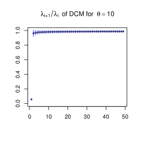
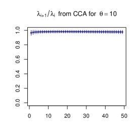
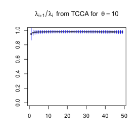
Figure 4.4: The average of the sequences of sample ratios $\{\lambda_{n,i+1}/\lambda_{n,i}\}$ from 1000 independent replications under Model 5 with $\theta=2,4$. Plots on the left panel are based on the DCM ${\mathbf{S}}_{xz}$, while those on the middle and right panels are based on CCA and TCCA, respectively. The dimensions are $(p,q,n)=(100,200,1000)$.

4.3 A consistent estimator for the order of finite-rank dependence

Assume that among the $m$ dependence strengths $(\theta_{k})_{1\leq k\leq m}:={\boldsymbol{\theta}}$, there are $m_{0}$ strengths above the critical value $\theta_{0}$ given in (4.3). According to Corollary 4.1, the $m_{0}$ largest eigenvalues $\lambda_{n,k}$ of the DCM ${\mathbf{S}}_{xz}$ will converge almost surely to $m_{0}$ limits $\lambda_{k}$, $1\leq k\leq m_{0}$, which are outside the support of $F$ and given in (4.4). Meanwhile, the following eigenvalues of any given number, say $s$, $\lambda_{n,m_{0}+1},\ldots,\lambda_{n,m_{0}+s}$ will all converge to the right edge $\lambda_{+}$ of the LSD $F$. The rank $m_{0}$ corresponds to the detectable rank of the weak dependence considered here. In a sense, the remaining $m-m_{0}$ dependence strengths $\{\theta_{m_{0}+1},\ldots,\theta_{m}\}$ below the critical value $\theta_{0}$ are too weak for detection. Following a popular ratio estimator for the number of factors or spikes developed in Onatski (2010) and Li et al. (2017), we introduce a consistent estimator for the detectable dependence rank $m_{0}$ in the model (4.1) as follows. Note that we have for $j=1,\ldots,m_{0}$, the ratios ${\lambda_{n,j+1}}/{\lambda_{n,j}}$ will converge almost surely to a number in $(0,1)$, while for $j\geq m_{0}+1$ these ratios will converge to 1. Let $0<d_{n}<1$ be a sequence of positive and vanishing constants and consider the following estimator for the dependence rank $m_{0}$:

$$\hat{m}_{0}=\{\text{first}~{}j\geq 1~{}~{}\text{such that }~{}\frac{\lambda_{n,j+1}}{\lambda_{n,j}}>1-d_{n}\}-1.$$

Under the conditions similar to Theorem 3.1 in Li et al. (2017), one can show that $\hat{m}_{0}$ will converge to $m_{0}$ almost surely.

It remains to set up an appropriate value for the tuning parameter $d_{n}$. Theoretically any vanishing sequence $d_{n}\to 0$ is sufficient for the consistence of $\hat{m}_{0}$. Here we follow the calibration proposed in Li et al. (2017). Precisely, we find empirically $q_{n,p,q,0.5\%}$, the lower 0.5% quantile of $\displaystyle n^{2/3}\big{(}\nu_{2}/\nu_{1}-1\big{)}$ where $\nu_{1}$ and $\nu_{2}$ are the top two sample eigenvalues of the distance covariance matrix ${\mathbf{S}}_{xy}$ under the null model with ${\mathbf{x}}\sim N({\bf 0},{\bf I}_{p})$ and ${\mathbf{y}}\sim N({\bf 0},{\bf I}_{q})$. Then we set $d_{n}=n^{-2/3}|q_{n,p,q,0.5\%}|$. Note that $d_{n}$ vanishes at rate $n^{-2/3}$. This tuned value of $d_{n}$ is used for all the simulation experiments in this section.

We now examine the performance of $\hat{m}_{0}$ in finite sample situations. Models 5 and 6 are adopted again when generating samples of ${\mathbf{x}}$ and ${\mathbf{y}}$. Under Model 5, we take $m=3$ and ${\boldsymbol{\theta}}=(4,3,2)$. The critical value $\theta_{0}$ is $1.2$, and thus the detectable dependence rank is $m_{0}=3$. Under Model 6, we take $m=4$ and ${\boldsymbol{\theta}}=(4,3,2,1)$. In this case $\theta_{0}=2.5$ and $m_{0}=2$. Frequencies of $\hat{m}_{0}$ are calculated from 1000 independent replications under the two models with the sample size $n$ ranging from 100 to 1600. The results are shown in Tables 4.2 and 4.3, which verify the convergence of the proposed estimator.

Table 4.2: Frequencies of $\hat{m}_{0}$ under Model 5 with ${\boldsymbol{\theta}}=(4,3,2)$ and $m_{0}=3$ from 1000 independent replications. The dimensional settings are $c_{n1}=0.1,c_{n2}=0.2$ and $n$ ranging from 100 to 1600.

	$\hat{m}_{0}=0$	$\hat{m}_{0}=1$	$\hat{m}_{0}=2$	$\hat{m}_{0}=3$	$\hat{m}_{0}=4$
$n=100$	0.045	0.649	0.293	0.013	0
$n=200$	0	0.144	0.676	0.176	0.004
$n=400$	0	0.020	0.406	0.561	0.013
$n=800$	0	0	0.057	0.942	0.001
$n=1600$	0	0	0	0.995	0.005

Table 4.3: Frequencies of $\hat{m}_{0}$ under Model 6 with ${\boldsymbol{\theta}}=(4,3,2,1)$ and $m_{0}=2$ from 1000 independent replications. The dimensional settings are $c_{n1}=1,c_{n2}=2$ and $n$ ranging from 100 to 1600.

	$\hat{m}_{0}=0$	$\hat{m}_{0}=1$	$\hat{m}_{0}=2$	$\hat{m}_{0}=3$
$n=100$	0.122	0.743	0.135	0
$n=200$	0.016	0.625	0.357	0.002
$n=400$	0	0.409	0.584	0.007
$n=800$	0	0.179	0.813	0.008
$n=1600$	0	0.039	0.953	0.008

Supplementary Materials

A supplementary to this article contains some additional technical tools used in this paper and the proofs of Theorem 2.1, Theorem 2.2, Theorem 3.1, Theorem 4.1 and Theorem 4.2.

School of Statistics and Management, Shanghai University of Finance and Economics E-mail: li.weiming@shufe.edu.cn

School of Data Science, Fudan University E-mail: wqw@fudan.edu.cn

Department of Statistics and Actuarial Science, The University of Hong Kong E-mail: jeffyao@hku.hk

Eigenvalue distribution of a high-dimensional

distance covariance matrix with application

Weiming Li, Qinwen Wang and Jianfeng Yao

Shanghai University of Finance and Economics,

Fudan University and The University of Hong Kong

Supplementary Material

This supplementary material contains some additional technical tools and the proofs of Theorem 2.1, Theorem 2.2, Theorem 3.1, Theorem 4.1 and Theorem 4.2 of the main paper. Throughout this supplementary material, $||\cdot||$ denotes the Euclidean norm for vectors, the spectral norm for matrices and the supremum norm for functions, respectively. ${\mathbb{C}}^{+}$ and ${\mathbb{C}}^{-}$ are referred as the upper and lower half complex plane (real axis excluded). $K$ is used to denote some constant that can vary from place to place.

Appendix A Technical tools

Lemma 1.

[El Karoui (2010)] Consider the $n\times n$ kernel random matrix ${\mathbf{M}}$ with entries

$${\mathbf{M}}_{i,j}=f\left(\frac{\|{\mathbf{x}}_{i}-{\mathbf{x}}_{j}\|^{2}_{2}}{p}\right).$$

Let us call $\boldsymbol{\psi}$ the vector with $i$-th entry $\boldsymbol{\psi}_{i}=\|{\mathbf{x}}_{i}\|^{2}_{2}/p-\tau/2$, where $\tau=2{\text{\rm tr}}({\bf\Sigma}_{p})/p$. We assume that:
(a) $n\asymp p$, that is, $n/p$ and $p/n$ remain bounded as $p\to\infty$.
(b) ${\bf\Sigma}_{p}$ is a positive semi-definite $p\times p$ matrix, and $\|{\bf\Sigma}_{p}\|=\sigma_{1}({\bf\Sigma}_{p})$ remains bounded in $p$, that is, there exists $K>0$, such that $\sigma_{1}({\bf\Sigma}_{p})\leq K$, for all $p$.
(c) There exists $\ell\in\mathbb{R}$ such that $\lim_{p\to\infty}{\text{\rm tr}}({\bf\Sigma}_{p})/p=\ell$.
(d) ${\mathbf{X}}=({\mathbf{x}}_{1},\ldots,{\mathbf{x}}_{n})$ and ${\mathbf{x}}_{i}={\bf\Sigma}^{1/2}_{p}{\mathbf{w}}_{i}$ for $i=1,\ldots,n$.
(e) The entries of ${\mathbf{w}}_{i}$, a $p$-dimensional random vector, are i.i.d. Also, denoting by $w_{ik}$ the $k$th entry of ${\mathbf{w}}_{i}$, we assume that ${\mathbb{E}}(w_{ik})=0$, ${\mathbb{V}}ar(w_{ik})=1$ and ${\mathbb{E}}(|w_{ik}|^{5+\varepsilon})<\infty$ for some $\varepsilon>0$.
(f) $f$ is $C^{3}$ in a neighborhood of $\tau$.
Then ${\mathbf{M}}$ can be approximated consistently in operator norm (and in probability) by the matrix $\widetilde{{\mathbf{M}}}$, defined by

$$\widetilde{{\mathbf{M}}} =f(\tau){\bf 1}{\bf 1}^{\prime}+{f}^{\prime}(\tau)\left[{\bf 1}\boldsymbol{\psi}^{\prime}+\boldsymbol{\psi}{{\bf 1}^{\prime}}-2\frac{{\mathbf{X}}^{\prime}{\mathbf{X}}}{p}\right]$$

$$\quad+\frac{f^{\prime\prime}(\tau)}{2}\left[{\bf 1}(\boldsymbol{\psi}\circ\boldsymbol{\psi})^{\prime}+(\boldsymbol{\psi}\circ\boldsymbol{\psi}){{\bf 1}^{\prime}}+2\boldsymbol{\psi}\boldsymbol{\psi}^{\prime}+4\frac{{\text{\rm tr}}({\bf\Sigma}^{2}_{p})}{p^{2}}{\bf 1}{\bf 1}^{\prime}\right]+v_{p}{\bf I}_{n},$$

$$v_{p} =f(0)+\tau f^{\prime}(\tau)-f(\tau).$$

In other words,

$$||{\mathbf{M}}-\widetilde{{\mathbf{M}}}||\to 0,\quad\text{in~{} probability}.$$

Lemma 2.

[Bai and Silverstein (2010)] Let ${\mathbf{A}}$ and ${\mathbf{B}}$ be two $n\times n$ Hermitian matrices. Then,

$$||F^{{\mathbf{A}}}-F^{{\mathbf{B}}}||\leq\frac{1}{n}{\rm rank}({\mathbf{A}}-{\mathbf{B}})\quad\text{and}\quad L^{3}(F^{\mathbf{A}},F^{\mathbf{B}})\leq\frac{1}{n}{\text{\rm tr}}[({\mathbf{A}}-{\mathbf{B}})({\mathbf{A}}-{\mathbf{B}})^{*}],$$

where $L(F,G)$ stands for the Lévy distance between the distribution functions $F$ and $G$.

Lemma 3.

Let $f$: $\mathbb{R}^{n}\to\mathbb{R}$ be any function of thrice differentiable in each argument. Let also ${\mathbf{x}}=(x_{1},\ldots,x_{n})^{\prime}$ and ${\mathbf{y}}=(y_{1},\ldots,y_{n})^{\prime}$ be two random vectors in $\mathbb{R}^{n}$ with i.i.d. elements, respectively, and set $U=f({\mathbf{x}})$ and $V=f({\mathbf{y}})$. If

$$\gamma=\max\{{\mathbb{E}}|x_{i}|^{3},{\mathbb{E}}|y_{i}|^{3},1\leq i\leq n\}<\infty,$$

then for any thrice differentiable $g:\mathbb{R}\to\mathbb{R}$ and any $K>0$,

$$|{\mathbb{E}}g(U)-{\mathbb{E}}g(V)|\leq 2C_{2}(g)\gamma n\lambda_{3}(f),$$

where $\lambda_{3}(f)=\sup\left\{|\partial^{k}_{i}f({\mathbf{z}})|^{3/k}:{\mathbf{z}}=(z_{\ell}),z_{\ell}\in\{x_{\ell},y_{\ell}\},1\leq i\leq n,1\leq k\leq 3\right\}$ and $C_{2}(g)=\frac{1}{6}\|g^{\prime}\|_{\infty}+\frac{1}{2}\|g^{\prime\prime}\|_{\infty}+\frac{1}{6}\|g^{\prime\prime\prime}\|_{\infty}$.

This lemma follows directly from Corollary 1.2 in Chatterjee (2008) and its proof.

Appendix B Proofs

At the beginning of this section, we first recall some notations for easy reading.

$${\mathbf{V}}_{x}=\left(\frac{\|{\bf x}_{k}-{\bf x}_{\ell}\|}{\sqrt{p}}\right),\quad{\mathbf{V}}_{y}=\left(\frac{\|{\bf y}_{k}-{\bf y}_{\ell}\|}{\sqrt{q}}\right),\quad{\bf P}_{n}={\mathbf{I}}_{n}-\frac{1}{n}{\bf 1}_{n}{\bf 1}_{n}^{\prime},$$

$$\gamma_{x}=\frac{1}{p}{\text{\rm tr}}{{\bf\Sigma}_{x}},~{}\quad\gamma_{y}=\frac{1}{q}{\text{\rm tr}}{\bf\Sigma}_{y},\quad\kappa_{x}=\frac{1}{pn}\sum_{i=1}^{n}||{\mathbf{x}}_{i}||^{2},\quad\kappa_{y}=\frac{1}{qn}\sum_{i=1}^{n}||{\mathbf{y}}_{i}||^{2},$$

$${\mathbf{A}}_{n}=\frac{1}{p}{\mathbf{X}}^{\prime}{\mathbf{X}}+\gamma_{x}{\bf I}_{n},~{}\quad{\mathbf{C}}_{n}=\frac{1}{q}{\mathbf{Y}}^{\prime}{\mathbf{Y}}+\gamma_{y}{\bf I}_{n},\quad{\mathbf{B}}_{n}={\mathbf{A}}_{n}^{\frac{1}{2}}{\mathbf{C}}_{n}{\mathbf{A}}_{n}^{\frac{1}{2}},$$

$${{\mathbf{D}}_{x}}=\frac{1}{p}{{\mathbf{X}}^{\prime}{\mathbf{X}}}+\kappa_{x}{{\mathbf{I}}_{n}},\quad{{\mathbf{D}}_{y}}=\frac{1}{q}{{\mathbf{Y}}^{\prime}{\mathbf{Y}}+\kappa_{y}{\mathbf{I}}_{n}},\quad{\mathbf{D}}_{z}=\frac{1}{q}{{\mathbf{Z}}^{\prime}{\mathbf{Z}}}+\kappa_{z}{\bf I}_{n},$$

$${\mathbf{S}}_{xy}={\bf P}_{n}{\mathbf{D}}_{x}{\bf P}_{n}{\mathbf{D}}_{y}{\bf P}_{n},\quad{\mathbf{S}}_{xz}={\mathbf{P}}_{n}{\mathbf{D}}_{x}{\mathbf{P}}_{n}{\mathbf{D}}_{z}{\mathbf{P}}_{n}.$$

B.1 Proof of Theorem 2.1

The squared sample distance covariance ${\mathcal{V}}^{2}_{n}({\bf x},{\bf y})$ in (1.2) can be expressed as an inner product between the two matrices ${\mathbf{P}}_{n}{\mathbf{V}}_{x}{\mathbf{P}}_{n}$ and ${\mathbf{P}}_{n}{\mathbf{V}}_{y}{\mathbf{P}}_{n}$, that is,

$${\mathcal{V}}_{n}^{2}({\bf x},{\bf y})=\frac{\sqrt{pq}}{n^{2}}{\text{\rm tr}}{\mathbf{P}}_{n}{\mathbf{V}}_{x}{\mathbf{P}}_{n}{\mathbf{V}}_{y}{\mathbf{P}}_{n}.$$

Notice that the matrices ${\mathbf{V}}_{x}$ and ${\mathbf{V}}_{y}$ are exactly the Euclidean distance kernel matrices discussed in El Karoui (2010) with kernel function $f(x)=\sqrt{x}$. Applying their main theorem (see Lemma 1), the matrix

$${\mathbf{P}}_{n}{\mathbf{V}}_{x}{\mathbf{P}}_{n}{\mathbf{V}}_{y}{\mathbf{P}}_{n}$$ (B.1)

can be approximated by a simplified random matrix ${\mathbf{V}}_{n}$ such that as $(n,p,q)$ tend to infinity,

$$\left\|{\mathbf{V}}_{n}-{\mathbf{P}}_{n}{\mathbf{V}}_{x}{\mathbf{P}}_{n}{\mathbf{V}}_{y}{\mathbf{P}}_{n}\right\|\to 0$$ (B.2)

in probability, where

$${\mathbf{V}}_{n}\triangleq\frac{1}{2\sqrt{\gamma_{x}\gamma_{y}}}{\mathbf{P}}_{n}\left({\mathbf{A}}_{n}+\frac{1}{8\gamma_{x}}\boldsymbol{\psi}_{x}\boldsymbol{\psi}^{\prime}_{x}\right){\mathbf{P}}_{n}\left({\mathbf{C}}_{n}+\frac{1}{8\gamma_{y}}\boldsymbol{\psi}_{y}\boldsymbol{\psi}^{\prime}_{y}\right){\mathbf{P}}_{n},$$ (B.3)

in which

$${\boldsymbol{\psi}_{x}}=\frac{1}{p}\left(\begin{array}[]{c}\|{\bf x}_{1}\|^{2}-{\text{\rm tr}}{\bf\Sigma}_{x}\\ \vdots\\ \|{\bf x}_{n}\|^{2}-{\text{\rm tr}}{\bf\Sigma}_{x}\end{array}\right)~{}~{}\text{and}~{}~{}\boldsymbol{\psi}_{y}=\frac{1}{q}\left(\begin{array}[]{c}\|{\bf y}_{1}\|^{2}-{\text{\rm tr}}{\bf\Sigma}_{y}\\ \vdots\\ \|{\bf y}_{n}\|^{2}-{\text{\rm tr}}{\bf\Sigma}_{y}\end{array}\right).$$ (B.10)

Then we replace the two traces $\gamma_{x}$ and $\gamma_{y}$ in ${\mathbf{A}}_{n}$ and ${\mathbf{C}}_{n}$ with their unbiased sample counterparts $\kappa_{x}$ and $\kappa_{y}$, respectively, which does not affect the convergence in (B.2). Finally in (B.3), by removing the two rank-one matrices $(8\gamma_{x})^{-1}\boldsymbol{\psi}_{x}\boldsymbol{\psi}^{T}_{x}$ and $(8\gamma_{y})^{-1}\boldsymbol{\psi}_{y}\boldsymbol{\psi}^{T}_{y}$ (which have bounded spectral norm, almost surely), we get the conclusion of the theorem. The proof is thus complete.

B.2 Proof of Theorem 2.2

Recall the approximation from Theorem 2.1,

$$\mathcal{V}^{2}_{n}({\bf x},{\bf y})=\frac{1}{2n^{2}}\sqrt{\frac{pq}{\gamma_{x}\gamma_{y}}}{\text{\rm tr}}{\mathbf{S}}_{xy}+o_{p}(1)$$

and notice that

$$\frac{1}{n}{\text{\rm tr}}({\mathbf{S}}_{xy}) =\frac{1}{npq}{\text{\rm tr}}({\mathbf{P}}_{n}{\mathbf{X}}^{\prime}{\mathbf{X}}{\mathbf{P}}_{n}{\mathbf{Y}}^{\prime}{\mathbf{Y}}{\mathbf{P}}_{n})+\frac{\kappa_{y}}{np}{\text{\rm tr}}({\mathbf{P}}_{n}{\mathbf{X}}^{\prime}{\mathbf{X}})+\frac{\kappa_{x}}{nq}{\text{\rm tr}}({\mathbf{P}}_{n}{\mathbf{Y}}^{\prime}{\mathbf{Y}})$$

$$\quad+\frac{n-1}{n}\kappa_{x}\kappa_{y}$$

$$=\frac{1}{npq}{\text{\rm tr}}({\mathbf{X}}^{\prime}{\mathbf{X}}{\mathbf{Y}}^{\prime}{\mathbf{Y}})+3\gamma_{x}\gamma_{y}+o_{a.s}(1).$$

Moreover, from Equation (21) in Li and Yao (2018) and the independence between ${\mathbf{X}}$ and ${\mathbf{Y}}$,

$$\frac{1}{npq}{\text{\rm tr}}({\mathbf{X}}^{\prime}{\mathbf{X}}{\mathbf{Y}}^{\prime}{\mathbf{Y}}) =\frac{1}{p}{\text{\rm tr}}({\bf\Sigma}_{x})\frac{1}{q}{\text{\rm tr}}({\bf\Sigma}_{y})+o_{a.s}(1).$$

Collecting the above results yields

$$\mathcal{V}^{2}_{n}({\bf x},{\bf y})=2\sqrt{c_{n1}c_{n2}\gamma_{x}\gamma_{y}}+o_{p}(1).$$

On the other hand, applying Lemma 1, we have

$$\frac{1}{n}S_{2,n}= \frac{1}{2n}\sqrt{\frac{pq}{\gamma_{x}\gamma_{y}}}\left(\frac{1}{n^{2}}{\bf 1}^{\prime}{\mathbf{D}}_{x}{\bf 1}-2\gamma_{x}\right)\left(\frac{1}{n^{2}}{\bf 1}^{\prime}{\mathbf{D}}_{y}{\bf 1}-2\gamma_{y}\right)+o_{p}\left(1\right)$$

$$= 2\sqrt{c_{n1}c_{n2}\gamma_{x}\gamma_{y}}+o_{p}(1).$$

Therefore, the statistic $T_{n}=n\mathcal{V}^{2}_{n}({\bf x},{\bf y})/S_{2,n}$ converges to 1 in probability. The proof is complete.

B.3 Proof of Theorem 3.1

The strategy of the proof is as follows. First, we prove the theorem under Gaussian assumption. By virtue of rotation invariance property of Gaussian vectors, we may treat the two population covariance matrices ${\bf\Sigma}_{x}$ and ${\bf\Sigma}_{y}$ as diagonal ones, which can simplify the proof dramatically. Second, applying Lindeberg’s replacement trick provided in Chatterjee (2008), we will remove the Gaussian assumption and show that the theorem still holds true for general distributions if the atoms $(w_{ij})$ have finite fourth moment, as stated in our Assumption (b).

Gaussian case: First, we have

$$|\kappa_{x}-\gamma_{x}|\xrightarrow{a.s.}0\quad\text{and}\quad|\kappa_{y}-\gamma_{y}|\xrightarrow{a.s.}0,$$ (B.11)

as $(n,p,q)$ tend to $\infty$. ¿From Lemma 2 and (B.11), we get

$$L^{3}(F^{{\mathbf{S}}_{xy}},F^{{\mathbf{B}}_{n}})\xrightarrow{a.s.}0.$$

Hence, the matrices ${\mathbf{S}}_{xy}$ and ${\mathbf{B}}_{n}$ share the same limiting spectral distribution and thus we only focus on the convergence of $F^{{\mathbf{B}}_{n}}$. We first derive its limit conditioning on the sequence $({\mathbf{A}}_{n})$. Then the result holds unconditionally if the limit is independent of $({\mathbf{A}}_{n})$. Following standard strategies from random matrix theory, letting $s_{{\mathbf{B}}_{n}}(z)$ be the Stieltjes transform of $F^{{\mathbf{B}}_{n}}$, the convergence of $F^{{\mathbf{B}}_{n}}$ can be established through three steps:

• Step 1: For any fixed $z\in\mathbb{C}^{+}$, $s_{{\mathbf{B}}_{n}}(z)-{\mathbb{E}}s_{{\mathbf{B}}_{n}}(z)\to 0$, almost surely.

• Step 2: For any fixed $z\in\mathbb{C}^{+}$, ${\mathbb{E}}s_{{\mathbf{B}}_{n}}(z)\to s(z)$ with $s(z)$ satisfies the equations in (3.1).

• Step 3: The uniqueness of the solution $s(z)$ to (3.1) on the set (3.2).

Step 1. Almost sure convergence of $s_{{\mathbf{B}}_{n}}(z)-{\mathbb{E}}s_{{\mathbf{B}}_{n}}(z)$.

We assume ${\bf\Sigma}_{y}$ is diagonal, having the form

$${\bf\Sigma}_{y}={\rm Diag}(\tau_{1},\ldots,\tau_{q}).$$

By this and notations

$${\mathbf{r}}_{k}=\frac{1}{\sqrt{q}}{\mathbf{A}}_{n}^{1/2}(w_{p+k,1},\ldots,w_{p+k,n})^{\prime},\quad k=1,\ldots,q,$$

the matrix ${\mathbf{B}}_{n}$ can be expressed as

$${\mathbf{B}}_{n}=\gamma_{y}{\mathbf{A}}_{n}+\sum_{k=1}^{q}\tau_{k}{\mathbf{r}}_{k}{\mathbf{r}}_{k}^{\prime}.$$ (B.12)

It’s “leave-one-out” version is denoted by ${\mathbf{B}}_{k,n}={\mathbf{B}}_{n}-\tau_{k}{\mathbf{r}}_{k}{\mathbf{r}}_{k}^{\prime}$, $k=1,\ldots,q$. Let ${\mathbb{E}}_{0}(\cdot)$ be expectation and ${\mathbb{E}}_{k}(\cdot)$ be conditional expectation given ${\mathbf{r}}_{1},\ldots,{\mathbf{r}}_{k}$. From the martingale decomposition and the identity

$${\mathbf{r}}_{k}^{\prime}({\mathbf{B}}_{n}-z{\mathbf{I}}_{n})^{-1}=\frac{{\mathbf{r}}_{k}^{\prime}({\mathbf{B}}_{k,n}-z{\mathbf{I}}_{n})^{-1}}{1+\tau_{k}{\mathbf{r}}_{k}^{\prime}({\mathbf{B}}_{k,n}-z{\mathbf{I}}_{n})^{-1}{\mathbf{r}}_{k}},$$ (B.13)

we have

$$s_{{\mathbf{B}}_{n}}(z)-{\mathbb{E}}s_{{\mathbf{B}}_{n}}(z)= \frac{1}{n}\sum_{k=1}^{q}({\mathbb{E}}_{k}-{\mathbb{E}}_{k-1})\left[{\text{\rm tr}}({\mathbf{B}}_{n}-z{\mathbf{I}}_{n})^{-1}-{\text{\rm tr}}({\mathbf{B}}_{k,n}-z{\mathbf{I}}_{n})^{-1}\right]$$

$$= -\frac{1}{n}\sum_{k=1}^{q}({\mathbb{E}}_{k}-{\mathbb{E}}_{k-1})\frac{\tau_{k}{\mathbf{r}}_{k}^{\prime}({\mathbf{B}}_{k,n}-z{\mathbf{I}}_{n})^{-2}{\mathbf{r}}_{k}}{1+\tau_{k}{\mathbf{r}}_{k}^{\prime}({\mathbf{B}}_{k,n}-z{\mathbf{I}}_{n})^{-1}{\mathbf{r}}_{k}}.$$ (B.14)

Similar to the arguments on pages 435-436 of Bai and Zhou (2008), the summands in (B.14) form a bounded martingale difference sequence, and hence $s_{{\mathbf{B}}_{n}}(z)-{\mathbb{E}}s_{{\mathbf{B}}_{n}}(z)\to 0$, almost surely.

Step 2. Convergence of ${\mathbb{E}}s_{{\mathbf{B}}_{n}}(z)$.

Let $s_{{\mathbf{A}}_{n}}(z)$ be the Stieltjes transform of $F^{{\mathbf{A}}_{n}}$. From Silverstein (1995), $s_{{\mathbf{A}}_{n}}(z)$ converges almost surely to $s_{\mathbf{A}}(z)$, which satisfies

$$z=-\frac{1}{s_{\mathbf{A}}(z)}+\int t+\frac{t}{1+tc_{1}^{-1}s_{\mathbf{A}}(z)}dH_{x}(t).$$ (B.15)

Define two functions $w_{n}(z)$ and $m_{n}(z)$ as

$$w_{n}(z)=\frac{1}{n}{\mathbb{E}}{\text{\rm tr}}({\mathbf{B}}_{n}-zI_{n})^{-1}{\mathbf{A}}_{n}\quad\text{and}\quad m_{n}(z)=\gamma_{y}+\frac{1}{q}\sum_{k=1}^{q}\frac{\tau_{k}}{1+\tau_{k}c_{n2}^{-1}w_{n}(z)}.$$ (B.16)

We first show that

$$m_{n}^{-1}(z)s_{{\mathbf{A}}_{n}}\left[zm_{n}^{-1}(z)\right]-{\mathbb{E}}s_{{\mathbf{B}}_{n}}(z)\to 0,\quad n\to\infty.$$ (B.17)

In fact, applying the identity (B.13), we have

$$\frac{1}{n}{\text{\rm tr}}\left[m_{n}(z){\mathbf{A}}_{n}-z{\mathbf{I}}_{n}\right]^{-1}-\frac{1}{n}{\text{\rm tr}}({\mathbf{B}}_{n}-z{\mathbf{I}}_{n})^{-1}$$

$$= \frac{1}{n}{\text{\rm tr}}\left[m_{n}(z){\mathbf{A}}_{n}-z{\mathbf{I}}_{n}\right]^{-1}\left(\sum_{k=1}^{q}\tau_{k}{\mathbf{r}}_{k}{\mathbf{r}}_{k}^{\prime}-(m_{n}(z)-\gamma_{y}){\mathbf{A}}_{n}\right)({\mathbf{B}}_{n}-z{\mathbf{I}}_{n})^{-1}$$

$$= \frac{1}{n}\sum_{k=1}^{q}\frac{\tau_{k}{\mathbf{r}}_{k}^{\prime}({\mathbf{B}}_{k,n}-zI_{n})^{-1}\left[(m_{n}(z){\mathbf{A}}_{n}-z{\mathbf{I}}_{n}\right]^{-1}{\mathbf{r}}_{k}}{1+\tau_{k}{\mathbf{r}}_{k}^{\prime}({\mathbf{B}}_{k,n}-z{\mathbf{I}}_{n})^{-1}{\mathbf{r}}_{k}}$$

$$-\frac{m_{n}(z)-\gamma_{y}}{n}{\text{\rm tr}}\left[m_{n}(z){\mathbf{A}}_{n}-z{\mathbf{I}}_{n}\right]^{-1}{\mathbf{A}}_{n}({\mathbf{B}}_{n}-z{\mathbf{I}}_{n})^{-1}$$

$$= \frac{1}{n}\sum_{k=1}^{q}\frac{\tau_{k}d_{k}}{1+\tau_{k}c_{n2}^{-1}w_{n}(z)},$$

where

$$d_{k}= \frac{1+\tau_{k}c_{n2}^{-1}w_{n}(z)}{1+\tau_{k}{\mathbf{r}}_{k}^{\prime}({\mathbf{B}}_{k,n}-z{\mathbf{I}}_{n})^{-1}{\mathbf{r}}_{k}}{\mathbf{r}}_{k}^{\prime}({\mathbf{B}}_{k,n}-z{\mathbf{I}}_{n})^{-1}\left[m_{n}(z){\mathbf{A}}_{n}-z{\mathbf{I}}_{n}\right]^{-1}{\mathbf{r}}_{k}$$

$$-\frac{1}{q}{\text{\rm tr}}\left[m_{n}(z){\mathbf{A}}_{n}-z{\mathbf{I}}_{n}\right]^{-1}{\mathbf{A}}_{n}({\mathbf{B}}_{n}-z{\mathbf{I}}_{n})^{-1}.$$

Following similar arguments on pages 85-87 of Bai and Silverstein (2010), one may obtain

$$\max_{k}{\mathbb{E}}(d_{k})\to 0.$$

This result together with the fact

$$\inf_{n}|1+\tau_{k}c_{n2}^{-1}w_{n}(z)|\geq\inf_{n}\tau_{k}c_{n2}^{-1}|\Im(w_{n}(z))|>0$$

imply the convergence in (B.17).

We next find another link between ${\mathbb{E}}s_{{\mathbf{B}}_{n}}(z)$ and $w_{n}(z)$ by proving

$$1+z{\mathbb{E}}s_{{\mathbf{B}}_{n}}(z)-\gamma_{y}w_{n}(z)-\frac{1}{n}\sum_{k=1}^{q}\frac{\tau_{k}w_{n}(z)}{c_{n2}+\tau_{k}w_{n}(z)}\to 0.$$ (B.18)

¿From the expression of ${\mathbf{B}}_{n}$ in (B.12) and the identity in (B.13), we have

$${\mathbf{I}}_{n}+z({\mathbf{B}}_{n}-z{\mathbf{I}})^{-1}= {\mathbf{B}}_{n}({\mathbf{B}}_{n}-z{\mathbf{I}}_{n})^{-1}$$

$$= \gamma_{y}{\mathbf{A}}_{n}({\mathbf{B}}_{n}-z{\mathbf{I}})^{-1}+\sum_{k=1}^{q}\tau_{k}{\mathbf{r}}_{k}{\mathbf{r}}_{k}^{\prime}({\mathbf{B}}_{n}-z{\mathbf{I}}_{n})^{-1}$$

$$= \gamma_{y}{\mathbf{A}}_{n}({\mathbf{B}}_{n}-z{\mathbf{I}})^{-1}+\sum_{k=1}^{q}\frac{\tau_{k}{\mathbf{r}}_{k}{\mathbf{r}}_{k}^{\prime}({\mathbf{B}}_{k,n}-z{\mathbf{I}}_{n})^{-1}}{1+\tau_{k}{\mathbf{r}}_{k}^{\prime}({\mathbf{B}}_{k,n}-z{\mathbf{I}}_{n})^{-1}{\mathbf{r}}_{k}}.$$ (B.19)

Taking the trace on both sides of (B.3) and dividing by $n$, we get

$$1+z\frac{1}{n}{\text{\rm tr}}({\mathbf{B}}_{n}-z{\mathbf{I}}_{n})^{-1}= \gamma_{y}\frac{1}{n}{\text{\rm tr}}({\mathbf{B}}_{n}-z{\mathbf{I}}_{n})^{-1}{\mathbf{A}}_{n}+\frac{1}{n}\sum_{k=1}^{q}\frac{\tau_{k}{\mathbf{r}}_{k}^{\prime}({\mathbf{B}}_{k,n}-z{\mathbf{I}}_{n})^{-1}{\mathbf{r}}_{k}}{1+\tau_{k}{\mathbf{r}}_{k}^{\prime}({\mathbf{B}}_{k,n}-z{\mathbf{I}}_{n})^{-1}{\mathbf{r}}_{k}}$$

$$= \gamma_{y}\frac{1}{n}{\text{\rm tr}}({\mathbf{B}}_{n}-z{\mathbf{I}}_{n})^{-1}{\mathbf{A}}_{n}+\frac{1}{n}\sum_{k=1}^{q}\frac{\tau_{k}c_{n2}^{-1}w_{n}(z)}{1+\tau_{k}c_{n2}^{-1}w_{n}(z)}+\varepsilon_{n},$$

where

$$\varepsilon_{n}=\frac{1}{n}\sum_{k=1}^{q}\frac{\tau_{k}[c_{n2}^{-1}w_{n}(z)-{\mathbf{r}}_{k}^{\prime}({\mathbf{B}}_{k,n}-z{\mathbf{I}}_{n})^{-1}{\mathbf{r}}_{k}]}{[1+\tau_{k}{\mathbf{r}}_{k}^{\prime}({\mathbf{B}}_{k,n}-z{\mathbf{I}}_{n})^{-1}{\mathbf{r}}_{k}][1+\tau_{k}c_{n2}^{-1}w_{n}(z)]}.$$

¿From the proof of (2.3) in Silverstein (1995), almost surely,

$$\inf_{n}\left|[1+\tau_{k}{\mathbf{r}}_{k}^{\prime}({\mathbf{B}}_{k,n}-z{\mathbf{I}}_{n})^{-1}{\mathbf{r}}_{k}][1+\tau_{k}c_{n2}^{-1}w_{n}(z)]\right|>0.$$

Moreover, following similar arguments on page 87 of Bai and Silverstein (2010), one may get

$$\frac{1}{n}\sum_{k=1}^{q}{\mathbb{E}}^{\frac{1}{2}}|c_{n2}^{-1}w_{n}(z)-{\mathbf{r}}_{k}^{\prime}({\mathbf{B}}_{k,n}-zI_{n})^{-1}{\mathbf{r}}_{k}|^{2}\to 0.$$

Therefore ${\mathbb{E}}(\varepsilon_{n})\to 0$ and hence the convergence in (B.18) holds.

By considering a subsequence $\{n_{k}\}$ such that $w_{n_{k}}(z)\to w(z)$, from (B.15), (B.17) and (B.18), we have

$$m_{n_{k}}(z) \to\int t+\frac{t}{1+tc_{n2}^{-1}w(z)}dH_{y}(t)\triangleq m(z),$$

$$s_{n_{k}}(z) \to\frac{1}{m(z)}s_{{\mathbf{A}}}\left(\frac{z}{m(z)}\right),$$

$$zs_{n_{k}}(z) \to-1+w(z)\int t+\frac{t}{1+tc_{2}^{-1}w(z)}dH_{y}(t),$$

as $k\to\infty$. These results demonstrate that $s_{n_{k}}(z)$ has a limit, say $s(z)$, which together with $(w(z),m(z)$, $s_{A}(z))$ satisfy the following system of equations:

$$\left\{\begin{array}[]{l}\displaystyle s(z)=\frac{1}{m(z)}s_{{\mathbf{A}}}\left(\frac{z}{m(z)}\right),\\ \displaystyle zs(z)=-1+w(z)\int t+\frac{t}{1+tc_{2}^{-1}w(z)}dH_{y}(t),\\ \displaystyle z=-\frac{1}{s_{\mathbf{A}}(z)}+\int t+\frac{t}{1+tc_{1}^{-1}s_{\mathbf{A}}(z)}dH_{x}(t),\\ \displaystyle m(z)=\int t+\frac{t}{1+tc_{2}^{-1}w(z)}dH_{y}(t).\end{array}\right.$$

Cancelling the function $s_{\mathbf{A}}(z)$ from the above system yields an equivalent but simpler system of equations as shown in (3.1). Hence, the convergence of $s_{n}(z)$ is established if the system has a unique solution on the set (3.2).

Step 3. Uniqueness of the solution to (3.1).

The system of equations in (3.1) is equivalent to

$$\left\{\begin{array}[]{l}\displaystyle 1+zs=wm,\\ \displaystyle m=\int t+\frac{t}{1+tc_{2}^{-1}w}dH_{y}(t),\\ \displaystyle w=s\int t+\frac{t}{1+tc_{1}^{-1}(1+zs)w^{-1}s}dH_{x}(t).\end{array}\right.$$ (B.23)

Bringing $s=[wm-1]/z$ into the third equation in (B.23), we have

$$w=\int\frac{t}{z}\Big{(}wm-1\Big{)}+\frac{t\big{(}wm-1\big{)}}{z+c_{1}^{-1}tm\big{(}wm-1\big{)}}dH_{x}(t).$$ (B.24)

Now suppose the LSD $F\neq\delta_{0}$ and we have two solutions $(s,w,m)$ and $(\tilde{s},\tilde{w},\tilde{m})$ to the system on the set (3.2) for a common $z\in\mathbb{C}^{+}$. Then, from (B.23) and (B.24), we can obtain

$$w-\tilde{w}=(wm-\tilde{w}\tilde{m})$$

$$\quad\quad\quad\quad\times\int\left[\frac{t}{z}+\frac{tz}{\big{(}z+c^{-1}_{1}tm(wm-1)\big{)}\big{(}z+c^{-1}_{1}t\tilde{m}(\tilde{w}\tilde{m}-1)\big{)}}\right]dH_{x}(t)$$

$$\quad\quad\quad\quad+(\tilde{m}-m)\int\frac{t^{2}c^{-1}_{1}(wm-1)(\tilde{w}\tilde{m}-1)}{(z+c^{-1}_{1}tm(wm-1))(z+c^{-1}_{1}t\tilde{m}(\tilde{w}\tilde{m}-1))}dH_{x}(t),$$ (B.25)

$$\tilde{m}-m=(w-\tilde{w})\int\frac{t^{2}c^{-1}_{2}}{\big{(}1+tc^{-1}_{2}w\big{)}\big{(}1+tc^{-1}_{2}\tilde{w}\big{)}}dH_{y}(t),$$ (B.26)

$$wm-\tilde{w}\tilde{m}=(w-\tilde{w})\int\left(t+\frac{t}{\big{(}1+tc^{-1}_{2}w\big{)}\big{(}1+tc^{-1}_{2}\tilde{w}\big{)}}\right)dH_{y}(t).~{}$$ (B.27)

Combining (B.25)-(B.27), if $w\neq\tilde{w}$, we have

$$B_{1}B_{2}+C_{1}C_{2}=1,$$ (B.28)

where

$$B_{1}=\int\frac{t}{z}+\frac{tz}{\big{(}z+c^{-1}_{1}tm(wm-1)\big{)}\big{(}z+c^{-1}_{1}t\tilde{m}(\tilde{w}\tilde{m}-1)\big{)}}dH_{x}(t),$$

$$B_{2}=\int t+\frac{t}{\big{(}1+tc^{-1}_{2}w\big{)}\big{(}1+tc^{-1}_{2}\tilde{w}\big{)}}dH_{y}(t),$$

$$C_{1}=\int\frac{t^{2}c^{-1}_{1}(wm-1)(\tilde{w}\tilde{m}-1)}{(z+c^{-1}_{1}tm(wm-1))(z+c^{-1}_{1}t\tilde{m}(\tilde{w}\tilde{m}-1))}dH_{x}(t),$$

$$C_{2}=\int\frac{t^{2}c^{-1}_{2}}{\big{(}1+tc^{-1}_{2}w\big{)}\big{(}1+tc^{-1}_{2}\tilde{w}\big{)}}dH_{y}(t).$$

By the Cauchy-Schwarz inequality, we have

$$|B_{1}B_{2}|^{2}\leq \int\Big{|}\frac{t}{z}\Big{|}+\frac{|tz|}{|z+c^{-1}_{1}tm(wm-1)|^{2}}dH_{x}(t)$$

$$\times\int\Big{|}\frac{t}{z}\Big{|}+\frac{|tz|}{|z+c^{-1}_{1}t\widetilde{m}(\widetilde{w}\widetilde{m}-1)|^{2}}dH_{x}(t)$$

$$\times\int t+\frac{t}{|1+tc^{-1}_{2}w|^{2}}dH_{y}(t)\int t+\frac{t}{|1+tc^{-1}_{2}\widetilde{w}|^{2}}dH_{y}(t)$$

$$= \int\Big{|}\frac{t}{z}\Big{|}+\frac{|tz|}{|z+c^{-1}_{1}tm(wm-1)|^{2}}dH_{x}(t)\int t+\frac{t}{|1+tc^{-1}_{2}w|^{2}}dH_{y}(t)$$

$$\times\int\Big{|}\frac{t}{z}\Big{|}+\frac{|tz|}{|z+c^{-1}_{1}t\widetilde{m}(\widetilde{w}\widetilde{m}-1)|^{2}}dH_{x}(t)\int t+\frac{t}{|1+tc^{-1}_{2}\widetilde{w}|^{2}}dH_{y}(t)$$

$$:= (\widetilde{B}_{1}\widetilde{B}_{2})^{2},$$

$$|C_{1}C_{2}|^{2}\leq \int\frac{t^{2}c^{-1}_{1}|wm-1|^{2}}{|z+c^{-1}_{1}tm(wm-1)|^{2}}dH_{x}(t)\int\frac{t^{2}c^{-1}_{1}|\widetilde{w}\widetilde{m}-1|^{2}}{|z+c^{-1}_{1}t\widetilde{m}(\widetilde{w}\widetilde{m}-1)|^{2}}dH_{x}(t)$$

$$\times\int\frac{t^{2}c^{-1}_{2}}{|1+tc^{-1}_{2}w|^{2}}dH_{y}(t)\frac{t^{2}c^{-1}_{2}}{|1+tc^{-1}_{2}\widetilde{w}|^{2}}dH_{y}(t)$$

$$= \int\frac{t^{2}c^{-1}_{1}|wm-1|^{2}}{|z+c^{-1}_{1}tm(wm-1)|^{2}}dH_{x}(t)\int\frac{t^{2}c^{-1}_{2}}{|1+tc^{-1}_{2}w|^{2}}dH_{y}(t)$$

$$\times\int\frac{t^{2}c^{-1}_{1}|\widetilde{w}\widetilde{m}-1|^{2}}{|z+c^{-1}_{1}t\widetilde{m}(\widetilde{w}\widetilde{m}-1)|^{2}}dH_{x}(t)\int\frac{t^{2}c^{-1}_{2}}{|1+tc^{-1}_{2}\widetilde{w}|^{2}}dH_{y}(t)$$

$$:= (\widetilde{C}_{1}\widetilde{C}_{2})^{2}.~{}$$

Then (B.28) implies

$$1 =|B_{1}B_{2}+C_{1}C_{2}|$$

$$\leq\sqrt{(\widetilde{B}^{2}_{1}+\widetilde{C}^{2}_{1})(\widetilde{B}^{2}_{2}+\widetilde{C}^{2}_{2})}$$

$$=\left\{\int\Big{|}\frac{t}{z}\Big{|}+\frac{|tz|}{|z+c^{-1}_{1}tm(wm-1)|^{2}}dH_{x}(t)\int t+\frac{t}{|1+tc^{-1}_{2}w|^{2}}dH_{y}(t)\right.$$

$$\quad\quad+\left.\int\frac{t^{2}c^{-1}_{1}|wm-1|^{2}}{|z+c^{-1}_{1}tm(wm-1)|^{2}}dH_{x}(t)\int\frac{t^{2}c^{-1}_{2}}{|1+tc^{-1}_{2}w|^{2}}dH_{y}(t)\right\}^{1/2}$$

$$\quad\times\left\{\int\Big{|}\frac{t}{z}\Big{|}+\frac{|tz|}{|z+c^{-1}_{1}t\widetilde{m}(\widetilde{w}\widetilde{m}-1)|^{2}}dH_{x}(t)\int t+\frac{t}{|1+tc^{-1}_{2}\widetilde{w}|^{2}}dH_{y}(t)\right.$$

$$\quad\quad+\left.\int\frac{t^{2}c^{-1}_{1}|\widetilde{w}\widetilde{m}-1|^{2}}{|z+c^{-1}_{1}t\widetilde{m}(\widetilde{w}\widetilde{m}-1)|^{2}}dH_{x}(t)\int\frac{t^{2}c^{-1}_{2}}{|1+tc^{-1}_{2}\widetilde{w}|^{2}}dH_{y}(t)\right\}^{1/2}.$$ (B.29)

On the other hand, taking the imaginary part on both sides of the second equation in (B.23) and (B.24), we obtain

$$\Im(\overline{m})=\int\frac{t^{2}c^{-1}_{2}\Im(w)}{|1+tc^{-1}_{2}w|^{2}}dH_{y}(t),$$ (B.30)

$$\Im(w)=\Im(wm\overline{z}-\overline{z})\int\frac{t}{|z|^{2}}+\frac{t}{|z+c^{-1}_{1}tm\big{(}wm-1\big{)}|^{2}}dH_{x}(t)$$

$$\quad\quad\quad+\Im(\overline{m})\int\frac{t^{2}c^{-1}_{1}|wm-1|^{2}}{|z+c^{-1}_{1}tm(wm-1)|^{2}}dH_{x}(t).$$ (B.31)

Further, if it holds

$$\Im(wm\overline{z}-\overline{z})>|z|\Im(w)\int t+\frac{t}{|1+tc^{-1}_{2}w|^{2}}dH_{y}(t),$$ (B.32)

then for $w\in\mathbb{C}^{+}$, combining the above three equations (B.30), (B.31) and (B.32) will lead to

$$1 >\int\frac{t}{|z|}+\frac{t|z|}{|z+c^{-1}_{1}tm\big{(}wm-1\big{)}|^{2}}dH_{x}(t)\int t+\frac{t}{|1+tc^{-1}_{2}w|^{2}}dH_{y}(t)$$

$$\quad\quad+\int\frac{t^{2}c^{-1}_{1}|wm-1|^{2}}{|z+c^{-1}_{1}tm(wm-1)|^{2}}dH_{x}(t)\int\frac{t^{2}c^{-1}_{2}}{|1+tc^{-1}_{2}w|^{2}}dH_{y}(t).$$ (B.33)

Such inequality also holds true if we replace $w$ and $m$ by $\tilde{w}$ and $\tilde{m}$, that is,

$$1 >\int\frac{t}{|z|}+\frac{t|z|}{|z+c^{-1}_{1}t\tilde{m}\big{(}\tilde{w}\tilde{m}-1\big{)}|^{2}}dH_{x}(t)\int t+\frac{t}{|1+tc^{-1}_{2}\tilde{w}|^{2}}dH_{y}(t)$$

$$\quad\quad+\int\frac{t^{2}c^{-1}_{1}|\tilde{w}\tilde{m}-1|^{2}}{|z+c^{-1}_{1}t\tilde{m}(\tilde{w}\tilde{m}-1)|^{2}}dH_{x}(t)\int\frac{t^{2}c^{-1}_{2}}{|1+tc^{-1}_{2}\tilde{w}|^{2}}dH_{y}(t).$$ (B.34)

Combining (B.3) and (B.3) will lead to a contradiction to (B.3), which means that we could only have one solution $(s,w,m)$ satisfying the system of equations (3.1) on the set (3.2).

So it is sufficient to prove the assertion (B.32) on some open set of $\mathbb{C}^{+}$. In fact, using the first and second equations in (B.23), we have

$$\Im(wm\overline{z}-\overline{z})=|z|^{2}\Im(s),$$

$$\Im(zs)=\Im(wm)=\int t+\frac{t}{|1+tc^{-1}_{2}w|^{2}}dH_{y}(t)\Im(w).$$

Then assertion (B.32) is equivalent to

$$\Im(s)>\frac{1}{|z|}\Im(zs).$$ (B.35)

Actually, for any subsequence $\{n_{k}\}$ such that

$$s_{n_{k}}(z)=\frac{1}{n_{k}}{\mathbb{E}}{\text{\rm tr}}({\mathbf{B}}_{n_{k}}-zI_{n})^{-1}$$

converges, the empirical distribution $F^{{\mathbf{B}}_{n_{k}}}$ has a limit $F$ (may depend on $\{n_{k}\}$), as $k\to\infty$, whose support is bounded upward by a constant, say $K$, which dose not depend on $\{n_{k}\}$. Moreover, the limit $s(z)$ of $s_{n_{k}}(z)$ is the Stieltjes transform of $F$, i.e.

$$s(z)=\int\frac{1}{x-z}dF(x).$$

This implies

$$\Im(s(z))=\int\frac{1}{|x-z|^{2}}dF(x)\Im(z),$$

$$\Im(zs(z))=\int\frac{x}{|x-z|^{2}}dF(x)\Im(z).$$

Therefore, (B.35) is true whenever $|z|>K$, which completes our proof.

Non-Gaussian case: since the two sets of samples $\{{\mathbf{x}}_{i}\}$ and $\{{\mathbf{y}}_{i}\}$ are independent, we first fix the sequence of matrices $({\mathbf{A}}_{n})$ and show that, without the Gaussian assumption, the empirical spectral distribution $F^{{\mathbf{S}}_{xy}}$ will still converge weakly to the same spectral distribution $F$ under Assumptions (a)-(c). Next, the same trick can be applied to $\{{\mathbf{x}}_{i}\}$, which will not be detailed here. Our strategy to remove the Gaussian assumption is based on Lemma 3, an extension of Lindeberg’s argument for general smooth functions, see also Corollary 1.2 in Chatterjee (2008). As a special case, letting $g$ be the identity function and $f$ be the Stieltjes transform, the theorem will ensure that the order of the difference in expectation between the two Stieltjes transforms under the Gaussian distribution and a non-Gaussian one is $O(n^{-1/2})$ whenever the two distributions match the first two moments and have finite fourth moment. Hence, such difference can be negligible as $n\to\infty$, by which and the “Step 1” for Gaussian case the proof is done.

Recall that

$${\mathbf{B}}_{n}={\mathbf{A}}^{1/2}_{n}\Big{(}\frac{1}{q}{\mathbf{Y}}^{\prime}{\mathbf{Y}}+\gamma_{y}{\mathbf{I}}\Big{)}{\mathbf{A}}^{1/2}_{n}={\mathbf{A}}^{1/2}_{n}\Big{(}\frac{1}{q}{\mathbf{W}}^{\prime}{\bf\Sigma}_{y}{\mathbf{W}}+\gamma_{y}I\Big{)}{\mathbf{A}}^{1/2}_{n},$$

where the table ${\mathbf{W}}$ consists i.i.d. standard Gaussian random variables and we vectorize it as a $qn$-dimensional random vector, denoted as ${\mathbf{w}}=(w_{ij})$. Therefore, the Stieltjes transform $s_{n}(z)$ of $F^{{\mathbf{B}}_{n}}$ can be viewed as a function of the random vector ${\mathbf{w}}$, defined as

$$U:=f({\mathbf{w}})=\frac{1}{n}{\text{\rm tr}}({\mathbf{B}}_{n}-z{\mathbf{I}})^{-1},$$

Similarly, we denote by

$$V:=f(\tilde{\mathbf{w}})$$

the non-Gaussian counterpart of $U$, where $\tilde{\mathbf{w}}=(\tilde{w}_{ij})$ have the same first two moments as $\{w_{ij}\}$ and finite fourth moment. Let $\bar{\mathbf{w}}=(\bar{w}_{ij})$ be a mixture of ${\mathbf{w}}$ and $\tilde{\mathbf{w}}$ by taking $\bar{w}_{ij}\in\{w_{ij},\tilde{w}_{ij}\}$ for $i=p+1,\ldots,p+q$ and $j=1,\ldots,n$, whose matrix form is denoted by $\mkern 1.5mu\overline{\mkern-1.5muW\mkern-1.5mu}\mkern 1.5mu$. Applying Lemma 3, one gets

$$|{\mathbb{E}}(U)-{\mathbb{E}}(V)|\leq Kqn\lambda_{3}(f),$$ (B.36)

where

$$\lambda_{3}(f)=\sup\left\{\bigg{|}\frac{\partial^{k}f(\bar{\mathbf{w}})}{\partial\bar{w}_{ij}^{k}}\bigg{|}^{3/k}:p+1\leq i\leq p+q,1\leq j\leq n,1\leq k\leq 3,\bar{\mathbf{w}}\in\mathbb{R}^{qn}\right\}.$$

Hence, the remaining work is to find a bound for $\lambda_{3}(f)$, which can be achieved from bounding the first three derivatives of $f$ with respect to $\bar{w}_{ij}$. To this end, following the same truncation, centralization and rescaling steps as in Bai and Silverstein (2010) (see Eq. (4.3.4)) and the “no eigenvalues” argument under finite fourth moment condition in Bai and Silverstein (1998), without loss of generality, we assume that the atoms $(\bar{w}_{ij})$ satisfy the following:

$${\mathbb{E}}(\bar{w}_{ij})=0,~{}{\mathbb{V}}ar(\bar{w}_{ij})=1,~{}|\bar{w}_{ij}|\leq\sqrt{n},~{}{{\mathbf{e}}_{i}^{\prime}\mkern 1.5mu\overline{\mkern-1.5mu{\mathbf{W}}\mkern-1.5mu}\mkern 1.5mu\mkern 1.5mu\overline{\mkern-1.5mu{\mathbf{W}}\mkern-1.5mu}\mkern 1.5mu^{\prime}{\mathbf{e}}_{i}\leq Kn,}$$

for all $i$ and $j$, where the vector ${\mathbf{e}}_{i}$ is the $i$th canonical basis on $\mathbb{R}^{q}$. For convenience, we still use notations $(w_{ij},{\mathbf{w}},{\mathbf{W}})$ instead of $(\bar{w}_{ij},\bar{\mathbf{w}},\mkern 1.5mu\overline{\mkern-1.5mu{\mathbf{W}}\mkern-1.5mu}\mkern 1.5mu)$ in what follows.

Let ${\mathbf{G}}=({\mathbf{B}}_{n}-zI)^{-1}$, then the first three derivatives of $f({\mathbf{w}})$ with respect to $w_{ij}$ are the following:

$$\frac{\partial f({\mathbf{w}})}{\partial w_{ij}}=\frac{1}{n}{\text{\rm tr}}{\mathbf{G}}^{\prime}=-\frac{1}{n}{\text{\rm tr}}{\mathbf{B}}^{\prime}_{n}{\mathbf{G}}^{2},$$

$$\frac{\partial^{2}f({\mathbf{w}})}{\partial w^{2}_{ij}}=-\frac{1}{n}{\text{\rm tr}}({\mathbf{B}}^{\prime\prime}_{n}{\mathbf{G}}^{2}+2{\mathbf{B}}^{\prime}_{n}{\mathbf{G}}{\mathbf{G}}^{\prime})=-\frac{1}{n}{\text{\rm tr}}{\mathbf{B}}^{\prime\prime}_{n}{\mathbf{G}}^{2}+\frac{2}{n}{\text{\rm tr}}{\mathbf{B}}^{\prime}_{n}{\mathbf{G}}^{2}{\mathbf{B}}^{\prime}_{n}{\mathbf{G}},$$

$$\frac{\partial^{3}f({\mathbf{w}})}{\partial w^{3}_{ij}}=\frac{4}{n}{\text{\rm tr}}{\mathbf{B}}^{\prime\prime}_{n}{\mathbf{G}}^{2}{\mathbf{B}}^{\prime}_{n}-\frac{6}{n}{\text{\rm tr}}{\mathbf{B}}^{\prime}_{n}{\mathbf{G}}^{2}{\mathbf{B}}^{\prime}_{n}{\mathbf{G}}{\mathbf{B}}^{\prime}_{n}{\mathbf{G}}+\frac{2}{n}{\text{\rm tr}}{\mathbf{B}}^{\prime}_{n}{\mathbf{G}}^{2}{\mathbf{B}}^{\prime\prime}_{n}{\mathbf{G}},$$

where

$${\mathbf{G}}^{\prime}=-{\mathbf{G}}{\mathbf{B}}^{\prime}_{n}{\mathbf{G}},$$

$${\mathbf{B}}^{\prime}_{n}=\frac{1}{q}{\mathbf{A}}^{1/2}_{n}({\mathbf{e}}_{j}{\mathbf{e}}^{\prime}_{i}{\bf\Sigma}_{y}{\mathbf{W}}+{\mathbf{W}}^{\prime}{\bf\Sigma}_{y}{\mathbf{e}}_{i}{\mathbf{e}}^{\prime}_{j}){\mathbf{A}}^{1/2}_{n},$$

$${\mathbf{B}}^{\prime\prime}_{n}=\frac{2}{q}{\mathbf{A}}^{1/2}_{n}{\mathbf{e}}_{j}{\mathbf{e}}^{\prime}_{i}{\bf\Sigma}_{y}{\mathbf{e}}_{i}{\mathbf{e}}^{\prime}_{j}{\mathbf{A}}^{1/2}_{n}.$$

and the vector ${\mathbf{e}}_{j}$ is the $j$th canonical basis on $\mathbb{R}^{n}$.

For the first derivative of $f$, since ${\bf\Sigma}_{y}$, ${\mathbf{A}}^{1/2}_{n}$ and ${\mathbf{G}}^{2}$ are all normal, we have

$$\sup\left|\frac{\partial f({\mathbf{w}})}{\partial w_{ij}}\right| \leq\sup\left\{\frac{1}{nq}\left|{\text{\rm tr}}{\mathbf{A}}^{1/2}_{n}{\mathbf{e}}_{j}{\mathbf{e}}^{\prime}_{i}{\bf\Sigma}_{y}{\mathbf{W}}{\mathbf{A}}^{1/2}_{n}{\mathbf{G}}^{2}\right|+\frac{1}{nq}\left|{\text{\rm tr}}{\mathbf{A}}^{1/2}_{n}{\mathbf{W}}^{\prime}{\bf\Sigma}_{y}{\mathbf{e}}_{i}{\mathbf{e}}^{\prime}_{j}{\mathbf{A}}^{1/2}_{n}{\mathbf{G}}^{2}\right|\right\}$$

$$\leq\sup\left\{\frac{K}{nq}\|{\mathbf{e}}_{j}\|\|{\mathbf{e}}^{\prime}_{i}{\mathbf{W}}\|+\frac{K}{nq}\|{\mathbf{W}}^{\prime}{\mathbf{e}}_{i}\|\|{\mathbf{e}}^{\prime}_{j}\|\right\}$$

$$\leq Kn^{-3/2}.$$ (B.37)

For the second derivative, we have

$$\left|\frac{1}{n}{\text{\rm tr}}{\mathbf{B}}^{\prime\prime}_{n}{\mathbf{G}}^{2}\right| =\frac{2}{nq}\left|{\text{\rm tr}}{\mathbf{A}}^{1/2}_{n}{\mathbf{e}}_{j}{\mathbf{e}}^{\prime}_{i}{\bf\Sigma}_{y}{\mathbf{e}}_{i}{\mathbf{e}}^{\prime}_{j}{\mathbf{A}}^{1/2}_{n}{\mathbf{G}}^{2}\right|\leq\frac{K}{nq}\|{\mathbf{e}}_{j}\|\cdot\|{\mathbf{e}}^{\prime}_{i}{\mathbf{e}}_{i}{\mathbf{e}}^{\prime}_{j}\|\leq Kn^{-2}~{}$$

and

$$\quad~{}\left|\frac{2}{n}{\text{\rm tr}}{\mathbf{B}}^{\prime}_{n}{\mathbf{G}}^{2}{\mathbf{B}}^{\prime}_{n}{\mathbf{G}}\right|$$

$$=\frac{2}{nq^{2}}\left|{\text{\rm tr}}{\mathbf{A}}^{1/2}_{n}({\mathbf{e}}_{j}{\mathbf{e}}^{\prime}_{i}{\bf\Sigma}_{y}{\mathbf{W}}+{\mathbf{W}}^{\prime}{\bf\Sigma}_{y}{\mathbf{e}}_{i}{\mathbf{e}}^{\prime}_{j}){\mathbf{A}}^{1/2}_{n}{\mathbf{G}}^{2}{\mathbf{A}}^{1/2}_{n}({\mathbf{e}}_{j}{\mathbf{e}}^{\prime}_{i}{\bf\Sigma}_{y}{\mathbf{W}}+{\mathbf{W}}^{\prime}{\bf\Sigma}_{y}{\mathbf{e}}_{i}{\mathbf{e}}^{\prime}_{j}){\mathbf{A}}^{1/2}_{n}{\mathbf{G}}\right|$$

$$\leq\frac{K}{nq^{2}}\left(\|{\mathbf{e}}_{j}\|\|{\mathbf{e}}^{\prime}_{i}{\mathbf{W}}{\mathbf{e}}_{j}{\mathbf{e}}^{\prime}_{i}{\mathbf{W}}\|+\|{\mathbf{e}}_{j}\|\|{\mathbf{e}}^{\prime}_{i}{\mathbf{W}}{\mathbf{W}}^{\prime}{\mathbf{e}}_{i}{\mathbf{e}}^{\prime}_{j}\|+\|{\mathbf{W}}^{\prime}{\mathbf{e}}_{i}\|\|{\mathbf{e}}^{\prime}_{j}{\mathbf{e}}_{j}{\mathbf{e}}^{\prime}_{i}{\mathbf{W}}\|+\|{\mathbf{W}}^{\prime}{\mathbf{e}}_{i}\|\|{\mathbf{e}}^{\prime}_{j}{\mathbf{W}}^{\prime}{\mathbf{e}}_{i}{\mathbf{e}}^{\prime}_{j}\|\right)$$

$$\leq\frac{K}{nq^{2}}\left(n+\sqrt{n}\cdot|w_{ij}|\right)$$

$$\leq Kn^{-2},$$

which leads to the conclusion that

$$\sup\left|\frac{\partial^{2}f({\mathbf{w}})}{\partial w^{2}_{ij}}\right|\leq Kn^{-2}.$$ (B.38)

Similarly, we could bound the third derivative as follows,

$$\sup\left|\frac{\partial^{3}f({\mathbf{w}})}{\partial w^{3}_{ij}}\right| \leq\sup\left\{\frac{K}{nq^{3}}\left(\|{\mathbf{e}}^{\prime}_{i}{\mathbf{W}}\||w_{ij}|^{2}+2|w_{ij}||{\mathbf{e}}_{i}^{\prime}{\mathbf{W}}{\mathbf{W}}^{\prime}{\mathbf{e}}_{i}|+\|{\mathbf{e}}^{\prime}_{i}{\mathbf{W}}\||{\mathbf{e}}_{i}^{\prime}{\mathbf{W}}{\mathbf{W}}^{\prime}{\mathbf{e}}_{i}|\right)\right.$$

$$\left.\quad+\frac{K}{nq^{2}}\left(\|{\mathbf{e}}^{\prime}_{i}{\mathbf{W}}\|+|w_{ij}|\right)\right\}$$

$$\leq Kn^{-5/2}.$$ (B.39)

Finally, combing (B.3), (B.38) and (B.3) gives

$$\lambda_{3}(f)=\sup\left\{\left|\frac{\partial f}{\partial w_{ij}}\right|^{3},\left|\frac{\partial^{2}f}{\partial w^{2}_{ij}}\right|^{\frac{3}{2}},\left|\frac{\partial^{3}f}{\partial w^{3}_{ij}}\right|\right\}=Kn^{-5/2},$$

which together with (B.36) imply

$$|{\mathbb{E}}(U)-{\mathbb{E}}(V)|\leq Kn^{-1/2}\to 0,\quad\text{as}\ n\to\infty.$$

The proof is done.

B.4 Proof of Theorem 4.1

Under our model setting (4.1), the three data matrices ${\mathbf{X}}$, ${\mathbf{Y}}$ and ${\mathbf{Z}}$ are related as:

$${\mathbf{Z}}=\Gamma{\mathbf{X}}{\mathbf{S}}+{\mathbf{Y}},$$

where $\Gamma=\sum_{k=1}^{m}\theta_{k}{\mathbf{u}}_{k}{\mathbf{v}}_{k}^{\prime}$ and ${\mathbf{S}}={\rm Diag}(\varepsilon_{1},\ldots,\varepsilon_{n})$. So we have

$$\frac{1}{q}{\mathbf{Z}}^{\prime}{\mathbf{Z}} =\frac{1}{q}{\mathbf{Y}}^{\prime}{\mathbf{Y}}+\frac{1}{q}{\mathbf{S}}{\mathbf{X}}^{\prime}\Gamma^{\prime}\Gamma{\mathbf{X}}{\mathbf{S}}+\frac{1}{q}{\mathbf{S}}{\mathbf{X}}^{\prime}\Gamma^{\prime}{\mathbf{Y}}+\frac{1}{q}{\mathbf{Y}}^{\prime}\Gamma{\mathbf{X}}{\mathbf{S}}$$

$$\triangleq\frac{1}{q}{\mathbf{Y}}^{\prime}{\mathbf{Y}}+{\mathbf{H}},$$

where

$${\mathbf{H}}=\frac{1}{q}{\mathbf{S}}{\mathbf{X}}^{\prime}\Gamma^{\prime}\Gamma{\mathbf{X}}{\mathbf{S}}+\frac{1}{q}{\mathbf{S}}{\mathbf{X}}^{\prime}\Gamma^{\prime}{\mathbf{Y}}+\frac{1}{q}{\mathbf{Y}}^{\prime}\Gamma{\mathbf{X}}{\mathbf{S}}$$ (B.40)

is a matrix of finite rank, at most $2m$. Denote

$$\widetilde{\mathbf{S}}_{xz}={\mathbf{A}}_{n}^{1/2}\left(\frac{1}{q}{\mathbf{Z}}^{\prime}{\mathbf{Z}}+\gamma_{z}{\mathbf{I}}_{n}\right){\mathbf{A}}_{n}^{1/2}\quad\text{and}\quad\widehat{\mathbf{S}}_{xz}={\mathbf{A}}_{n}^{1/2}\left(\frac{1}{q}{\mathbf{Y}}^{\prime}{\mathbf{Y}}+\gamma_{z}{\mathbf{I}}_{n}\right){\mathbf{A}}_{n}^{1/2},\quad$$

where

$$\gamma_{z}={\frac{1}{q}}{\text{\rm tr}}({\bf\Sigma}_{z})=\gamma_{y}+\frac{1}{q}\sum_{i=1}^{m}\theta^{2}_{i}\cdot\gamma_{x}=\gamma_{y}+o(1).$$ (B.41)

Applying Lemma 2 to ${\mathbf{B}}_{n}$, $\widetilde{\mathbf{S}}_{xz}$ and $\widehat{\mathbf{S}}_{xz}$, we have

$$||F^{\widetilde{\mathbf{S}}_{xz}}-F^{\widehat{\mathbf{S}}_{xz}}||\to 0\quad\text{and}\quad L^{3}(F^{{\mathbf{B}}_{n}},F^{\widehat{\mathbf{S}}_{xz}})\to 0,$$ (B.42)

almost surely, as $(n,p,q)$ tend to infinty. Combining (B.42) and the fact that $\widetilde{\mathbf{S}}_{xz}$ shares the same LSD as ${\mathbf{S}}_{xz}$, we conclude that $F^{{\mathbf{S}}_{xz}}$ converges weakly to the LSD $F$ defined by (3.1). The proof is thus complete.

B.5 Proof of Theorem 4.2

We first note that, from the convergence in (B.11) and (B.41), asymptotically, the largest eigenvalues of ${\mathbf{S}}_{xz}$ are the same as those of

$$\bar{\mathbf{S}}_{xz}:={\mathbf{A}}^{1/2}_{n}\left(\frac{1}{q}{\mathbf{Y}}^{\prime}{\mathbf{Y}}+{\mathbf{H}}+\gamma_{y}{\mathbf{I}}_{n}\right){\mathbf{A}}^{1/2}_{n},$$

where ${\mathbf{H}}$ is given in (B.40). So it’s equivalent to prove the theorem for $\bar{\mathbf{S}}_{xz}$.

Next, from Bai and Silverstein (1998) and the inequality

$$||{\mathbf{A}}^{1/2}_{n}{\mathbf{C}}_{n}{\mathbf{A}}^{1/2}_{n}||\leq||{\mathbf{A}}_{n}||\cdot||{\mathbf{C}}_{n}||,$$

we know that the spectral norm $||{\mathbf{A}}^{1/2}_{n}{\mathbf{C}}_{n}{\mathbf{A}}^{1/2}_{n}||$ is bounded in $n$, almost surely. Define

$$\lambda_{+}=\limsup_{n\to\infty}||{\mathbf{A}}^{1/2}_{n}{\mathbf{C}}_{n}{\mathbf{A}}^{1/2}_{n}||,$$

we consider the existence of spiked eigenvalues $(\lambda_{n,\ell})$ of $\bar{\mathbf{S}}_{xz}$ in the interval $(\lambda_{+},+\infty)$. That is, for each $\ell\in\{1,\ldots,k\}$, $\lambda_{n,\ell}$ is an eigenvalue of $\bar{\mathbf{S}}_{xz}$ but not an eigenvalue of ${\mathbf{A}}^{1/2}_{n}{\mathbf{C}}_{n}{\mathbf{A}}^{1/2}_{n}$, i.e.

$$\left|\lambda{\mathbf{I}}_{n}-\bar{\mathbf{S}}_{xz}\right|=0\quad\text{and}\quad\left|\lambda{\mathbf{I}}_{n}-{\mathbf{A}}^{1/2}_{n}{\mathbf{C}}_{n}{\mathbf{A}}^{1/2}_{n}\right|\neq 0,$$ (B.43)

for $\lambda\in\{\lambda_{n,1},\ldots,\lambda_{n,k}\}$.

In the following, we will show the limits of $\lambda$ is defined in (4.4). Under the assumptions in (B.43), we have

$$\left|{\mathbf{I}}_{n}-\left(\lambda{\mathbf{I}}_{n}-{\mathbf{A}}^{1/2}_{n}{\mathbf{C}}_{n}{\mathbf{A}}^{1/2}_{n}\right)^{-1}{\mathbf{A}}^{1/2}_{n}{\mathbf{H}}{\mathbf{A}}^{1/2}_{n}\right|=0.$$ (B.44)

Recall the definition of ${\mathbf{H}}$ in (B.40), then with a little bit calculation, this matrix can be decomposed as

$${\mathbf{H}}=\frac{1}{q}\left(\begin{array}[]{ccccc}{\mathbf{a}}_{1}&{\mathbf{b}}_{1}&\cdots&{\mathbf{a}}_{m}&{\mathbf{b}}_{m}\end{array}\right)\left(\begin{array}[]{ccccc}\theta_{1}\lambda_{11}&0&\cdots&0&0\\ 0&\theta_{1}\lambda_{12}&\cdots&0&0\\ \vdots&\vdots&\ddots&\vdots&\vdots\\ 0&0&\cdots&\theta_{m}\lambda_{m1}&0\\ 0&0&\cdots&0&\theta_{m}\lambda_{m2}\end{array}\right)\left(\begin{array}[]{c}{\mathbf{a}}^{\prime}_{1}\\ {\mathbf{b}}^{\prime}_{1}\\ \vdots\\ {\mathbf{a}}^{\prime}_{m}\\ {\mathbf{b}}^{\prime}_{m}\\ \end{array}\right),$$ (B.56)

where

$${\mathbf{a}}_{i} =u_{i1}{\mathbf{S}}{\mathbf{X}}^{\prime}{\mathbf{v}}_{i}+w_{i1}{\mathbf{Y}}^{\prime}{\mathbf{u}}_{i},$$

$${\mathbf{b}}_{i} =u_{i2}{\mathbf{S}}{\mathbf{X}}^{\prime}{\mathbf{v}}_{i}+w_{i2}{\mathbf{Y}}^{\prime}{\mathbf{u}}_{i},$$

$$\lambda_{i1} =\|{\mathbf{S}}{\mathbf{X}}^{\prime}{\mathbf{v}}_{i}\|\|{\mathbf{Y}}^{\prime}{\mathbf{u}}_{i}\|\left\{\frac{\sqrt{4\|{\mathbf{Y}}^{\prime}{\mathbf{u}}_{i}\|^{2}+\theta^{2}_{i}\|{\mathbf{S}}{\mathbf{X}}^{\prime}{\mathbf{v}}_{i}\|^{2}}+\theta_{i}\|{\mathbf{S}}{\mathbf{X}}^{\prime}{\mathbf{v}}_{i}\|}{\sqrt{4\|{\mathbf{Y}}^{\prime}{\mathbf{u}}_{i}\|^{2}+\theta^{2}_{i}\|{\mathbf{S}}{\mathbf{X}}^{\prime}{\mathbf{v}}_{i}\|^{2}}-\theta_{i}\|{\mathbf{S}}{\mathbf{X}}^{\prime}{\mathbf{v}}_{i}\|}\right\}^{1/2},$$

$$\lambda_{i2} =-\|{\mathbf{S}}{\mathbf{X}}^{\prime}{\mathbf{v}}_{i}\|\|{\mathbf{Y}}^{\prime}{\mathbf{u}}_{i}\|\left\{\frac{\sqrt{4\|{\mathbf{Y}}^{\prime}{\mathbf{u}}_{i}\|^{2}+\theta^{2}_{i}\|{\mathbf{S}}{\mathbf{X}}^{\prime}{\mathbf{v}}_{i}\|^{2}}-\theta_{i}\|{\mathbf{S}}{\mathbf{X}}^{\prime}{\mathbf{v}}_{i}\|}{\sqrt{4\|{\mathbf{Y}}^{\prime}{\mathbf{u}}_{i}\|^{2}+\theta^{2}_{i}\|{\mathbf{S}}{\mathbf{X}}^{\prime}{\mathbf{v}}_{i}\|^{2}}+\theta_{i}\|{\mathbf{S}}{\mathbf{X}}^{\prime}{\mathbf{v}}_{i}\|}\right\}^{1/2},$$

with

$$u_{i1}=\frac{1}{\|{\mathbf{S}}{\mathbf{X}}^{\prime}{\mathbf{v}}_{i}\|}\left\{\frac{1}{2}+\frac{\theta_{i}\|{\mathbf{S}}{\mathbf{X}}^{\prime}{\mathbf{v}}_{i}\|}{2\sqrt{4\|{\mathbf{Y}}^{\prime}{\mathbf{u}}_{i}\|^{2}+\theta^{2}_{i}\|{\mathbf{S}}{\mathbf{X}}^{\prime}{\mathbf{v}}_{i}\|^{2}}}\right\}^{1/2},$$

$$u_{i2}=\frac{1}{\|{\mathbf{S}}{\mathbf{X}}^{\prime}{\mathbf{v}}_{i}\|}\left\{\frac{1}{2}-\frac{\theta_{i}\|{\mathbf{S}}{\mathbf{X}}^{\prime}{\mathbf{v}}_{i}\|}{2\sqrt{4\|{\mathbf{Y}}^{\prime}{\mathbf{u}}_{i}\|^{2}+\theta^{2}_{1}\|{\mathbf{S}}{\mathbf{X}}^{\prime}{\mathbf{v}}_{i}\|^{2}}}\right\}^{1/2},$$

$$w_{i1}=\frac{1}{\|{\mathbf{Y}}^{\prime}{\mathbf{u}}_{i}\|}\left\{\frac{1}{2}-\frac{\theta_{i}\|{\mathbf{S}}{\mathbf{X}}^{\prime}{\mathbf{v}}_{i}\|}{2\sqrt{4\|{\mathbf{Y}}^{\prime}{\mathbf{u}}_{i}\|^{2}+\theta^{2}_{i}\|{\mathbf{S}}{\mathbf{X}}^{\prime}{\mathbf{v}}_{i}\|^{2}}}\right\}^{1/2},$$

$$w_{i2}=-\frac{1}{\|{\mathbf{Y}}^{\prime}{\mathbf{u}}_{i}\|}\left\{\frac{1}{2}+\frac{\theta_{i}\|{\mathbf{S}}{\mathbf{X}}^{\prime}{\mathbf{v}}_{i}\|}{2\sqrt{4\|{\mathbf{Y}}^{\prime}{\mathbf{u}}_{i}\|^{2}+\theta^{2}_{i}\|{\mathbf{S}}{\mathbf{X}}^{\prime}{\mathbf{v}}_{i}\|^{2}}}\right\}^{1/2}.$$

In addition, it’s straightforward to verify the following relations,

$$\left\{\begin{array}[]{l}\displaystyle\lambda_{i1}u^{2}_{i1}+\lambda_{i2}u^{2}_{i2}=\theta_{i},\\ \displaystyle\lambda_{i1}w^{2}_{i1}+\lambda_{i2}w^{2}_{i2}=0,\\ \displaystyle\lambda_{i1}u_{i1}w_{i1}+\lambda_{i2}u_{i2}w_{i2}=1.\end{array}\right.$$ (B.60)

Denote ${\mathbf{D}}_{n}={\mathbf{A}}^{1/2}_{n}\left(\lambda{\mathbf{I}}_{n}-{\mathbf{A}}^{1/2}_{n}{\mathbf{C}}_{n}{\mathbf{A}}^{1/2}_{n}\right)^{-1}{\mathbf{A}}^{1/2}_{n}$ and

$${\mathbf{M}}_{n}=\frac{1}{q}\left(\begin{array}[]{c}{\mathbf{a}}^{\prime}_{1}\\ {\mathbf{b}}^{\prime}_{1}\\ \vdots\\ {\mathbf{a}}^{\prime}_{m}\\ {\mathbf{b}}^{\prime}_{m}\\ \end{array}\right){\mathbf{D}}_{n}\left(\begin{array}[]{ccccc}{\mathbf{a}}_{1}&{\mathbf{b}}_{1}&\cdots&{\mathbf{a}}_{m}&{\mathbf{b}}_{m}\end{array}\right)\left(\begin{array}[]{ccccc}\theta_{1}\lambda_{11}&0&\cdots&0&0\\ 0&\theta_{1}\lambda_{12}&\cdots&0&0\\ \vdots&\vdots&\ddots&\vdots&\vdots\\ 0&0&\cdots&\theta_{m}\lambda_{m1}&0\\ 0&0&\cdots&0&\theta_{m}\lambda_{m2}\end{array}\right).$$

Then (B.44) and (B.56) imply

$$f_{n}(\lambda):=|{\mathbf{I}}_{2m}-{\mathbf{M}}_{n}|=0.$$

We next find the limit of $f_{n}(\lambda)$. Let

$$\alpha_{n}=\frac{1}{n}{\text{\rm tr}}{\mathbf{S}}{\mathbf{D}}_{n}{\mathbf{S}}({\mathbf{A}}_{n}-\gamma_{x}{\mathbf{I}}_{n})\quad\text{and}\quad\beta_{n}=\frac{1}{n}{\text{\rm tr}}{\mathbf{D}}_{n}({\mathbf{C}}_{n}-\gamma_{y}{\mathbf{I}}_{n}),$$

one may get for any $i\in\{1,\ldots,m\}$,

$$\frac{{\mathbf{a}}^{\prime}_{i}{\mathbf{D}}_{n}{\mathbf{a}}_{i}}{q}=\frac{u_{i1}^{2}}{c_{n2}}\alpha_{n}+\frac{w_{i1}^{2}}{c_{n2}}\beta_{n}+o_{a.s.}(1),$$

$$\frac{{\mathbf{a}}^{\prime}_{i}{\mathbf{D}}_{n}{\mathbf{b}}_{i}}{q}=\frac{u_{i1}u_{i2}}{c_{n2}}\alpha_{n}+\frac{w_{i1}w_{i2}}{c_{n2}}\beta_{n}+o_{a.s.}(1),$$

$$\frac{{\mathbf{b}}^{\prime}_{i}{\mathbf{D}}_{n}{\mathbf{b}}_{i}}{q}=\frac{u_{i2}^{2}}{c_{n2}}\alpha_{n}+\frac{w_{i2}^{2}}{c_{n2}}\beta_{n}+o_{a.s.}(1)~{},$$

and for any $i\neq j\in\{1,\ldots,m\}$,

$$\frac{{\mathbf{a}}^{\prime}_{i}{\mathbf{D}}_{n}{\mathbf{a}}_{j}}{q}=o_{a.s.}(1)~{},\quad\frac{{\mathbf{a}}^{\prime}_{i}{\mathbf{D}}_{n}{\mathbf{b}}_{j}}{q}=o_{a.s.}(1)~{}.$$

¿From the above approximations and the identities in (B.60), we have

$$f_{n}(\lambda)=\prod_{k=1}^{m}\big{|}{\mathbf{I}}_{2}-{\mathbf{M}}_{nk}\big{|}+o_{a.s}(1)$$

where

$${\mathbf{M}}_{nk}=\frac{\theta_{k}}{c_{n2}}\left(\begin{array}[]{cc}\alpha_{n}&0\\ 0&\beta_{n}\end{array}\right)\left(\begin{array}[]{cc}\theta_{k}&1\\ 1&0\end{array}\right).$$ (B.65)

Let ${\boldsymbol{\varepsilon}}=(\varepsilon_{1},\ldots,\varepsilon_{n})^{\prime}$, then

$$\alpha_{n}=\frac{1}{n}{\text{\rm tr}}{\mathbf{S}}{\mathbf{D}}_{n}{\mathbf{S}}{\mathbf{A}}_{n}-\frac{\gamma_{x}}{n}{\text{\rm tr}}{\mathbf{S}}{\mathbf{D}}_{n}{\mathbf{S}}=\frac{1}{n}{\boldsymbol{\varepsilon}}^{\prime}\left({\mathbf{D}}_{n}\circ{\mathbf{A}}_{n}\right){\boldsymbol{\varepsilon}}-\frac{\gamma_{x}}{n}{\boldsymbol{\varepsilon}}^{\prime}\text{Diag}({\mathbf{D}}_{n}){\boldsymbol{\varepsilon}},$$ (B.66)

where “$\circ$” denotes the Hadamard product of two matrices. According to Theorem 1 of Varberg (1968), we have

$$\frac{1}{n}{\boldsymbol{\varepsilon}}^{\prime}\left({\mathbf{D}}_{n}\circ{\mathbf{A}}_{n}\right){\boldsymbol{\varepsilon}}-\frac{1}{n}{\mathbb{E}}\left[{\boldsymbol{\varepsilon}}^{\prime}\left({\mathbf{D}}_{n}\circ{\mathbf{A}}_{n}\right){\boldsymbol{\varepsilon}}\right]\xrightarrow{a.s.}0,$$ (B.67)

$$\frac{1}{n}{\boldsymbol{\varepsilon}}^{\prime}\text{Diag}({\mathbf{D}}_{n}){\boldsymbol{\varepsilon}}-\frac{1}{n}{\mathbb{E}}{\text{\rm tr}}{\mathbf{D}}_{n}\xrightarrow{a.s.}0.$$ (B.68)

Further,

$$~{}\quad\frac{1}{n}{\mathbb{E}}\left[{\boldsymbol{\varepsilon}}^{\prime}\left({\mathbf{D}}_{n}\circ{\mathbf{A}}_{n}\right){\boldsymbol{\varepsilon}}\right]=\frac{1}{n}{\mathbb{E}}{\text{\rm tr}}\big{[}{\mathbf{D}}_{n}\text{Diag}({\mathbf{A}}_{n})\big{]}$$

$$=\frac{1}{n}{\mathbb{E}}{\text{\rm tr}}\big{[}{\mathbf{D}}_{n}\left(\text{Diag}({\mathbf{A}}_{n})-2\gamma_{x}{\mathbf{I}}_{n}\right)\big{]}+\frac{2\gamma_{x}}{n}{\mathbb{E}}{\text{\rm tr}}{\mathbf{D}}_{n}$$

$$=\frac{2\gamma_{x}}{n}{\mathbb{E}}{\text{\rm tr}}{\mathbf{D}}_{n}+o(1),$$ (B.69)

where the last equality is due to the following convergence,

$$\left|\frac{1}{n}{\text{\rm tr}}\big{[}{\mathbf{D}}_{n}\cdot\left(\text{Diag}({\mathbf{A}}_{n})-2\gamma_{x}{\mathbf{I}}_{n}\right)\big{]}\right|\leq\frac{1}{n}\|{\mathbf{D}}_{n}\|\cdot{\text{\rm tr}}\big{|}{\mathbf{A}}_{n}-2\gamma_{x}{\mathbf{I}}_{n}\big{|}\xrightarrow{a.s.}0.$$

Collecting results in (B.66)-(B.5), we get

$$\alpha_{n}=-\gamma_{x}w_{n}(\lambda)+o_{a.s.}(1)\xrightarrow{a.s.}\alpha\triangleq-w(\lambda)\int tdH_{x}(t),$$ (B.70)

where $w_{n}(z)$ is defined in (B.16), whose domain can be expanded to $(\lambda_{+},+\infty)$ for all large $n$. For $\beta_{n}$, we have

$$\beta_{n} =\frac{1}{n}{\text{\rm tr}}({\mathbf{D}}_{n}{\mathbf{C}}_{n})-\frac{\gamma_{y}}{n}{\text{\rm tr}}{\mathbf{D}}_{n}$$

$$=-1+\frac{\lambda}{n}{\text{\rm tr}}\left(\lambda{\mathbf{I}}_{n}-{\mathbf{A}}^{1/2}_{n}{\mathbf{C}}_{n}{\mathbf{A}}^{1/2}_{n}\right)^{-1}-\frac{\gamma_{y}}{n}{\text{\rm tr}}{\mathbf{D}}_{n}$$

$$=-\frac{1}{n}\sum_{k=1}^{q}\frac{\tau_{k}w_{n}(\lambda)}{c_{n2}+\tau_{k}w_{n}(\lambda)}+o_{a.s.}(1)$$

$$\xrightarrow{a.s.}\beta\triangleq-c_{2}\int\frac{tw(\lambda)dH_{y}(t)}{c_{2}+tw(\lambda)},$$ (B.71)

where the third equality is from (B.18) with $(\tau_{k})$ being the eigenvalues of ${\bf\Sigma}_{y}$. Collecting results in (B.65),(B.70) and (B.71), we get

$$f_{n}(\lambda)\xrightarrow{a.s.}f(\lambda)\triangleq\prod_{k=1}^{m}\left(1-\theta_{k}^{2}g(\lambda)\right),$$

where the function $g$ is given in (4.2). With the definition of the critical value $\theta_{0}$ in (4.3), we find that for any $k\in\{1,\ldots,m\}$ and $\theta_{k}>\theta_{0}$, there are $k$ zeros $\lambda_{1}>\cdots>\lambda_{k}$ of $f(\lambda)$ on $(\lambda_{+},\infty)$. By continuity arguments, see Lemma 6.1 in Benaych-Georges and Nadakuditi (2011), we verify the existence of the spikes $\lambda_{n,1},\ldots,\lambda_{n,k}$ whose limits are $\lambda_{1},\ldots,\lambda_{k}$, respectively. The proof is then complete.

References

- Bai and Silverstein (1998) Bai, Z.D. and Silverstein, J.W. (1998) No eigenvalues outside the support of the limiting spectral distribution of large dimensional random matrices. Ann. Probab., 26, 316–345.