ItôTTS and ItôWave: Linear Stochastic Differential Equation Is All You Need For Audio Generation

Abstract

In this paper, we propose to unify the two aspects of voice synthesis, namely text-to-speech (TTS) and vocoder, into one framework based on a pair of forward and reverse-time linear stochastic differential equations (SDE). The solutions of this SDE pair are two stochastic processes, one of which turns the distribution of mel spectrogram (or wave), that we want to generate, into a simple and tractable distribution. The other is the generation procedure that turns this tractable simple signal into the target mel spectrogram (or wave). The model that generates mel spectrogram is called ItôTTS, and the model that generates wave is called ItôWave. ItôTTS and ItôWave use the Wiener process as a driver to gradually subtract the excess signal from the noise signal to generate realistic corresponding meaningful mel spectrogram and audio respectively, under the conditional inputs of original text or mel spectrogram. The results of the experiment show that the mean opinion scores (MOS) of ItôTTS and ItôWave can exceed the current state-of-the-art methods, and reached 3.925$\pm$0.160 and 4.35$\pm$0.115 respectively. The generated audio samples are available at https://shiziqiang.github.io/ito_audio/.

All authors contribute equally to this work.

1 Introduction

In recent years, the generation technology, especially the voice generation technology has made great progress. Voice generation technology consists of two important and relatively independent modules, one is text-to-speech (TTS) and the other is vocoder. Among them, TTS transforms text into voice features, such as mel spectrogram, and vocoder transforms voice features into waveforms. Most researchers study TTS and vocoder separately, and design for different characteristics of different tasks.

Whether it is a TTS or a vocoder, the model is roughly categorized as autoregressive (AR) or non-autoregressive (non-AR), where the AR model generates the signal frame by frame, and the generation of the current signal frame depends on the previously generated signal. Non-AR models generate the signal in parallel, and the current signal frame does not depend on the previous signal. Generally speaking, the voice quality generated by the AR model is higher than the non-AR model, but the amount of computation is also larger, and the generation speed is slow. While for the non-AR generation model, the generation speed is faster, but the generated voice quality is slightly worse. To name a few, for example, in the field of TTS, AR-type models are generally implemented through the framework of encoder and decoder, and the duration of text is predicted by an attention module, such as Tacotron [36] and Tacotron 2 [28], DeepVoice 2 [7] and 3 [22]. In the last two years, most of the work has focused on the study of non-AR TTS models, such as flow based models [34, 18, 12], variational auto-encoder (VAE) based models [16], generative adversarial network (GAN) based models [2], and Fastspeech and Fastspeech 2 [25, 26] etc.

The situation in the vocoder field is similar. WaveNet [19] is the earliest AR model, using sampling points as the unit and achieves a sound quality that matches the naturalness of human speech. In addition, other recent AR models, including sampleRNN [17] and LPCNet [33] have further improved the sound quality. However, due to the large amount of computation and the slow generation speed, researchers currently mainly focus on developing non-AR wave generation models, such as Parallel WaveNet [20], ClariNet [21], GanSynth [5], FloWaveNet [11], MelGan [15], WaveGlow [24], Parallel WaveGan [37], and so on.

In this paper, TTS and vocoder are modeled with the same new framework based on linear Itô stochastic differential equations (SDE) and score matching modeling. We call them ItôTTS and ItôWave respectively. The linear Itô SDE, driven by the Wiener process, can slowly turn the mel spectrogram and wave data distributions, that need to be generated in TTS and vocoder, into data distributions that are easy to manipulate, such as white noise. This transformation process is the stochastic process solution of the linear Itô SDE. Therefore, the corresponding reverse-time linear Itô SDE can generate the mel spectrogram and wave data distribution required by TTS and vocoder, from this easy data distribution, such as white noise. It can be seen that the reverse-time linear Itô SDE is crucial for the generation, and Anderson [1] shows the explicit form of this reverse-time linear SDE, and the formula shows that it depends on the gradient of the log value of the probability density function of the stochastic process solution of the forward-time equation. This gradient value is also called the stein score [9]. ItôTTS and ItôWave predict the stein score corresponding to the mel spectrogram or wave by trained neural networks. After obtaining this score, ItôTTS and ItôWave can achieve the goal of generating mel spectrogram and wave through reverse-time linear Itô SDE or Langevin dynamic sampling.

Our contribution is as follows:

• We are among the first to proposed a TTS and vocoder model based on linear Itô SDE, called ItôTTS and ItôWave, which reached state-of-the-art performance. These models are easier to train than the GAN-based models and do not require a reversible network like the flow models.

• We explicitly unify TTS and vocoder under a more flexible framework, which can construct different TTS and vocoder models by selecting different drift and diffusion coefficients of the linear SDE.

• For ItôTTS and ItôWave, we propose two network structures, which are suitable for estimating the gradient of log value of the density function of the mel spectrogram and wave data distributions.

• It is believed that ItôTTS and ItôWave provide many knowhows, serves as a good and new high starting baseline, and there will be more linear SDE-based sound generation work in the future.

2 Related work

The earliest source of the ideas for ItôTTS and ItôWave should be the pioneering change of data estimation problem into the estimation of the gradient of log of the data distribution density by Hyvärinen and Dayan [9], thus greatly simplifying the original problem. Another source is the pioneering use of a diffusion Markov chain by Sohl-Dickstein et al. [29] to diffuse the structure of the image data into a simple distribution, and another opposite diffusion Markov chain to generate images in the target distribution from the simple distribution. In the past two years, these two primitive ideas have been carried forward.  Ho et al. [8] has recently generated very high-quality large-scale natural images with a diffusion Markov chain. DiffWave [14] uses a diffusion Markov chain for the vocoder.  Song and Ermon [30] draws on the idea of  [9] to estimate the log gradient of the target data distribution density function through a neural network, and then uses the Langevin dynamics to generate large-scale image data in target distribution. Wavegrad [3] transplanted the algorithm of Song and Ermon [30] to vocoders, but in fact the final algorithm is exactly the same as Diffwave [14]. Immediately afterward,  Song et al. [31] further extended the Markov chain to the continuous case, it became a stochastic differential equation. Ingeniously, the equation unified the two methods of Ho et al. [8] and Song and Ermon [30] under one framework, and both became its special cases.

ItôTTS and ItôWave successfully found the realization of the linear SDE framework in sound generation and achieved very high-quality sound.

3 ItôTTS and ItôWave

3.1 Audio data distribution transformation based on Itô SDE

Itô SDE is a very natural model that can realize the transformation between different data distributions. The general Itô SDE is as follows

$$\left\{\begin{array}[]{lr}d\mathbf{X}=\mathbf{f}(\mathbf{X},t)dt+g(t)d\mathbf{W}&\\ \mathbf{X}(0)=\mathbf{x}(0)&\end{array}\right.$$ (3)

for $0\leq t\leq T$, where $\mathbf{f}(\cdot,t)$ is the drift coefficient, $g(t)$ is the diffusion coefficient, $\mathbf{W}$ is the standard Wiener process. The solution of this Itô SDE is a stochastic process $\mathbf{X}(t)$ satisfies the following Itô integrals

$$\mathbf{X}(t)=\mathbf{x}(0)+\int_{0}^{t}\mathbf{f}(\mathbf{X}(s),s)ds+\int_{0}^{t}g(s)d\mathbf{W}(s)$$ (4)

all most surely for all $0\leq t\leq T$. Let $p(\mathbf{x}(t))$ be the density of the random variable $\mathbf{X}(t)$. This SDE (3) changes the initial distribution $p(\mathbf{x}(0))$ into another distribution $p(\mathbf{x}(T))$ by gradually adding the noise from the Wiener process $\mathbf{W}$. In this work, $\mathbf{x}(t)\in\mathbb{R}^{d}$, and $p(\mathbf{x}(0))$ is to denote the data distribution of mel spectrogram or wave in ItôTTS or ItôWave respectively. $p(\mathbf{x}(T))$ is an easy tractable distribution (e.g. Gaussian) of the latent representation of the mel spectrogram or wave signal corresponding to the conditional text or mel spectrogram. If this stochastic process $\mathbf{x}(t)$ can be reversed in time, then the target mel spectrogram or waveform of the corresponding text or mel spectrogram can be generated from a simple latent distribution.

Actually the reverse-time diffusion process is the solution of the following corresponding reverse-time Itô SDE [1]

$$\left\{\begin{array}[]{lr}d\mathbf{X}=\left[\mathbf{f}(\mathbf{X},t)-g(t)^{2}\nabla_{\mathbf{x}}\log p(\mathbf{x}(t))\right]dt+g(t)d\overline{\mathbf{W}}&\\ \mathbf{X}(T)=\mathbf{x}(T)&\end{array}\right.$$ (7)

for $0\leq t\leq T$, where $p(\mathbf{x}(t))$ is the distribution of $\mathbf{X}(t)$, $\overline{\mathbf{W}}$ is the standard Wiener process in reverse-time. The solution of this reverse-time Itô SDE (7) can be used to generate mel spectrogram or wave data from a tractable latent distribution $p(\mathbf{x}(T))$. Therefore, it can be seen from (7) that the key to generating mel spectrogram or wave with SDE lies in the calculations of $\nabla_{\mathbf{x}}\log p(\mathbf{x}(t))$ $(0\leq t\leq T)$, which is always called score function [9, 30] of the data.

3.2 Score estimation of audio data distribution

In this work, a neural network $\mathfrak{S}_{\theta}$ is used to approximate the score function, where $\theta$ denotes the parameters of the network. The input of the network $\mathfrak{S}_{\theta}$ includes time $t$, $\mathbf{x}(t)$, and conditional input text $\mathbf{p}$ or mel spectrograms $\mathbf{m}$ in ItôTTS and ItôWave respectively. The expected output is $\nabla_{\mathbf{x}(t)}\log p(\mathbf{x}(t))$. The objective of score matching is [9] (here we only take ItôWave as an example, the situation of ItôTTS is almost the same)

$$\mathbb{E}_{t\sim[0,T]}\mathbb{E}_{\mathbf{x}(t)\sim p(\mathbf{x}(t))}\left[\frac{1}{2}\parallel\mathfrak{S}_{\theta}(\mathbf{x}(t),t,\mathbf{m})-\nabla_{\mathbf{x}(t)}\log p(\mathbf{x}(t))\parallel^{2}\right].$$ (8)

Generally speaking, in the low-density data manifold area, the score estimation will be inaccurate, which will further lead to the low quality of the sampled data [30]. If the mel spectrogram or wave signal is contaminated with a very small scale noise, then the contaminated mel spectrogram or wave signal will spread to the entire space $\mathbb{R}^{d}$ instead of being limited to a small low-dimensional manifold. When using perturbed mel spectrogram or wave signal as input, the following denoising score matching (DSM) loss [35, 30]

$$\text{DSM loss}=\mathbb{E}_{t\sim[0,T]}\mathbb{E}_{\mathbf{x}(0)\sim p_{mel}(\mathbf{x}(0))}\mathbb{E}_{\mathbf{x}(t)\sim p(\mathbf{x}(t)|\mathbf{x}(0))}\left[\frac{1}{2}\parallel\mathfrak{S}_{\theta}(\mathbf{x}(t),t,\mathbf{m})-\nabla_{\mathbf{x}(t)}\log p(\mathbf{x}(t)|\mathbf{x}(0))\parallel^{2}\right].$$ (9)

is equal to the loss (8) of a non-parametric (e.g. Parzen windows densiy) estimator [35]. This DSM loss is used in this paper to train the score prediction network. If we can accurately estimate the score $\nabla_{\mathbf{x}(t)}\log p(\mathbf{x}(t))$ of the distribution, then we can generate mel spectrogram or wave sample data from the original distribution.

It should be noted that in the experiment we found that the choice of training loss is very critical. For ItôTTS, the $\mathcal{L}1$ loss is more suitable, and for ItôWave, the $\mathcal{L}2$ loss is more appropriate. The intuition is that the frequency mel-spectrogram data favors $\mathcal{L}1$-loss, while time-domain wave data favors $\mathcal{L}2$-loss.

Generally the transition densities $p(\mathbf{x}(t)|\mathbf{x}(0))$ and $\nabla_{\mathbf{x}(t)}\log p(\mathbf{x}(t)|\mathbf{x}(0))$ in the DSM loss are difficult to calculate, but for linear SDE, these values have close formulas [27].

3.3 Linear SDE and transition densities

Linear SDE refers to such an equation

$$\left\{\begin{array}[]{lr}d\mathbf{X}=\left[\mathbf{C}(t)\mathbf{X}+\mathbf{d}(t)\right]dt+g(t)\mathbf{I}d\mathbf{W}&\\ \mathbf{X}(0)=\mathbf{x}(0).&\end{array}\right.$$ (12)

where $\mathbf{C}(t)\in\mathbb{R}^{d\times d}$ and $\mathbf{d}(t)\in\mathbb{R}^{d}$.

The transition densities $p(\mathbf{x}(t)|\mathbf{x}(0))$ of the solution process $\mathbf{X}(t)$ for the SDE (12) is the solution to the Fokker-Planck-Kolmogorov (FPK) equation [27]

$$\frac{\partial p(\mathbf{x}(t),t)}{\partial t}=-\sum_{i=1}^{d}\frac{\partial\left[\mathbf{C}(t)\mathbf{x}+\mathbf{d}(t)\right]}{\partial x_{i}}+\sum_{i=1}^{d}\sum_{j=1}^{d}\frac{\partial^{2}}{\partial x_{i}\partial x_{j}}[g(t)^{2}p(\mathbf{x}(t),t)],$$ (13)

which in this case can derive that $p(\mathbf{x}(t)|\mathbf{x}(0))$ is Gaussian with mean $\mathbf{m}(t)$ and variance $\mathbf{V}(t)$ satisfy the ordinary equations [27]

$$\left\{\begin{array}[]{lr}\frac{d\mathbf{m}(t)}{dt}=\mathbf{C}(t)\mathbf{m}(t)+\mathbf{d}(t)&\\ \frac{d\mathbf{V}(t)}{dt}=\mathbf{C}(t)\mathbf{V}(t)+\mathbf{V}(t)\mathbf{C}(t)^{T}+g(t)^{2}\mathbf{I}.&\end{array}\right.$$ (16)

Empirically it is found that different types of linear SDE for different audio generation tasks, e.g. the variance exploding (VE) SDE [31] is much suitable for wave generation, while variance preserving (VP) SDE [31] is more suitable mel-spectrogram generation. VE SDE is of the following form

$$\left\{\begin{array}[]{lr}d\mathbf{X}=\sigma_{0}(\frac{\sigma_{1}}{\sigma_{0}})^{t}\sqrt{2\log\frac{\sigma_{1}}{\sigma_{0}}}d\mathbf{W}&\\ \mathbf{X}(0)=\mathbf{x}(0)\sim\int p_{mel}(\mathbf{x})\mathcal{N}(\mathbf{x}(0);\mathbf{x},\sigma_{0}^{2}\mathbf{I})d\mathbf{x},&\end{array}\right.$$ (19)

where $\sigma_{0}=0.01<\sigma_{1}$.

Then the differential equation satisfied by the mean and variance of the transition densities $p(\mathbf{x}(t)|\mathbf{x}(0))$ is as follows

$$\left\{\begin{array}[]{lr}\frac{d\mathbf{m}(t)}{dt}=\mathbf{0}&\\ \frac{d\mathbf{V}(t)}{dt}=2\sigma^{2}_{0}(\frac{\sigma_{1}}{\sigma_{0}})^{2t}\log\frac{\sigma_{1}}{\sigma_{0}}\mathbf{I}.&\end{array}\right.$$ (22)

Solving the above equation, and choose $\sigma_{1}$ makes $2\log\frac{\sigma_{1}}{\sigma_{0}}=1$, we get the transition density of this as

$$p(\mathbf{x}(t)|\mathbf{x}(0))=\mathcal{N}\left(\mathbf{x}(t);\mathbf{x}(0),\left[\sigma_{0}^{2}(\frac{\sigma_{1}}{\sigma_{0}})^{2t}-\sigma_{0}^{2}\right]\mathbf{I}\right).$$ (23)

The score of the VE linear SDE is

$$\nabla_{\mathbf{x}(t)}\log p(\mathbf{x}(t)|\mathbf{x}(0))=\nabla_{\mathbf{x}(t)}\log\mathcal{N}\left(\mathbf{x}(t);\mathbf{x}(0),\left[\sigma_{0}^{2}(\frac{\sigma_{1}}{\sigma_{0}})^{2t}-\sigma_{0}^{2}\right]\mathbf{I}\right)$$

$$=\nabla_{\mathbf{x}(t)}\left[-\frac{d}{2}\log\left[2\pi\left(\sigma_{0}^{2}(\frac{\sigma_{1}}{\sigma_{0}})^{2t}-\sigma_{0}^{2}\right)\right]-\frac{\parallel\mathbf{x}(t)-\mathbf{x}(0)\parallel^{2}}{2\left(\sigma_{0}^{2}(\frac{\sigma_{1}}{\sigma_{0}})^{2t}-\sigma_{0}^{2}\right)}\right]=-\frac{\mathbf{x}(t)-\mathbf{x}(0)}{\sigma_{0}^{2}(\frac{\sigma_{1}}{\sigma_{0}})^{2t}-\sigma_{0}^{2}}.$$ (24)

The prior distribution $p(\mathbf{x}(T))$ is a Gaussian

$$\mathcal{N}\left(\mathbf{x}(T);\mathbf{0},\sigma_{1}^{2}\mathbf{I}\right)=\frac{\exp(-\frac{1}{2\sigma_{1}^{2}}\left\lVert\mathbf{x}(T)\right\rVert^{2})}{\sigma_{1}^{d}\sqrt{(2\pi)^{d}}},$$ (25)

thus $\log p(\mathbf{x}(T))=-\frac{d}{2}\log(2\pi\sigma_{1}^{2})-\frac{1}{2\sigma_{1}^{2}}\left\lVert\mathbf{x}(T)\right\rVert^{2}$.

The VP linear SDE is

$$\left\{\begin{array}[]{lr}d\mathbf{X}=-\frac{1}{2}(\beta_{0}+t(\beta_{1}-\beta_{0}))\mathbf{X}dt+\sqrt{\beta_{0}+t(\beta_{1}-\beta_{0})}d\mathbf{W}&\\ \mathbf{X}(0)=\mathbf{x}(0)\sim p_{mel}(\mathbf{x}),&\end{array}\right.$$ (28)

where $\beta_{1}>\beta_{0}$ are constant hyperparameters. Then the differential equation satisfied by the mean and variance of the transition densities $p(\mathbf{x}(t)|\mathbf{x}(0))$ is as follows

$$\left\{\begin{array}[]{lr}\frac{d\mathbf{m}(t)}{dt}=-\frac{1}{2}(\beta_{0}+t(\beta_{1}-\beta_{0}))\mathbf{m}(t)&\\ \frac{d\mathbf{V}(t)}{dt}=-(\beta_{0}+t(\beta_{1}-\beta_{0}))\mathbf{V}(t)+(\beta_{0}+t(\beta_{1}-\beta_{0}))\mathbf{I}.&\end{array}\right.$$ (31)

By solving the above linear ordinary differential equations with initial conditions that $\mathbf{m}(0)=\mathbf{x}(0)$ and $\mathbf{V}(0)=\mathbf{x}(0)$, we obtain

$$\left\{\begin{array}[]{lr}\mathbf{m}(t)=\mathbf{x}(0)\exp{\left[-\frac{1}{2}\beta_{0}t-\frac{1}{4}t^{2}(\beta_{1}-\beta_{0})\right]}&\\ \mathbf{V}(t)=\mathbf{I}-\mathbf{I}\exp{\left[-\beta_{0}t-\frac{1}{2}t^{2}(\beta_{1}-\beta_{0})\right]}.&\end{array}\right.$$ (34)

we get the transition density of this as

$$p(\mathbf{x}(t)|\mathbf{x}(0))=\mathcal{N}\left(\mathbf{x}(t);\mathbf{x}(0)\exp{\left[-\frac{1}{2}\beta_{0}t-\frac{1}{4}t^{2}(\beta_{1}-\beta_{0})\right]},\mathbf{I}-\mathbf{I}\exp{\left[-\beta_{0}t-\frac{1}{2}t^{2}(\beta_{1}-\beta_{0})\right]}\right).$$ (35)

The score of the VP linear SDE is

$$\nabla_{\mathbf{x}(t)}\log p(\mathbf{x}(t)|\mathbf{x}(0))$$

$$=\nabla_{\mathbf{x}(t)}\left[-\frac{d}{2}\log\left[2\pi\left(1-\exp{\left[-\beta_{0}t-\frac{1}{2}t^{2}(\beta_{1}-\beta_{0})\right]}\right)\right]-\frac{\parallel\mathbf{x}(t)-\mathbf{x}(0)\exp{\left[-\frac{1}{2}\beta_{0}t-\frac{1}{4}t^{2}(\beta_{1}-\beta_{0})\right]}\parallel^{2}}{2\left(1-\exp{\left[-\beta_{0}t-\frac{1}{2}t^{2}(\beta_{1}-\beta_{0})\right]}\right)}\right]$$

$$=-\frac{\mathbf{x}(t)-\mathbf{x}(0)\exp{\left[-\frac{1}{2}\beta_{0}t-\frac{1}{4}t^{2}(\beta_{1}-\beta_{0})\right]}}{1-\exp{\left[-\beta_{0}t-\frac{1}{2}t^{2}(\beta_{1}-\beta_{0})\right]}}.$$ (36)

The prior distribution $p(\mathbf{x}(T))$ is a Gaussian

$$\mathcal{N}\left(\mathbf{x}(T);\mathbf{0},\mathbf{I}\right)=\frac{\exp(-\frac{1}{2}\left\lVert\mathbf{x}(T)\right\rVert^{2})}{\sqrt{(2\pi)^{d}}},$$ (37)

thus $\log p(\mathbf{x}(T))=-\frac{d}{2}\log(2\pi)-\frac{1}{2}\left\lVert\mathbf{x}(T)\right\rVert^{2}$.

In this paper, we use the VE linear SDE for wave generation and the VP linear SDE for mel-spectrogram generation. In future work, we will develop other types of linear SDEs that are suitable for audio generation, and discover the principles that can determine which type of SDE is more appropriate for audio generation.

3.4 Training algorithms

Based on subsections 3.1 and 3.2, we can get the training algorithm of the score networks based on general SDEs. Here we have taken the training algorithm of ItôTTS as an example, as shown below

Algorithm 1 Training of the score network in general SDE-based mel spectrogram generation model

Input and initialization: The mel spectrogram $\mathbf{x}$ and the corresponding text condition $\mathbf{p}$, the diffusion time $T$.

1: for $k=0,1,\cdots$

2:  Uniformly sample $t$ from $[0,T]$.

3:   Randomly sample batch of $\mathbf{x}$ and $\mathbf{p}$, let $\mathbf{x}(0)=\mathbf{x}$, compute to sample $\mathbf{x}(t)$ and $\nabla_{\mathbf{x}(t)}\log p(\mathbf{x}(t)|\mathbf{x}(0))$, then average the following

$$\text{DSM }loss=\parallel\mathfrak{S}_{\theta_{k}}(\mathbf{x}(t),t,\mathbf{p})-\nabla_{\mathbf{x}(t)}\log p(\mathbf{x}(t)|\mathbf{x}(0))\parallel_{1}.$$

4:   Do the back-propagation and the parameter updating of $\mathfrak{S}_{\theta}$.

5:  $k\leftarrow k+1$.

6: Until stopping conditions are satisfied and $\mathfrak{S}_{\theta_{k}}$ converges, e.g. to $\mathfrak{S}_{\theta_{*}}$.

Output: $\mathfrak{S}_{\theta_{*}}$.

In the above subsection 3.3, for VE linear SDE, we have obtained the closed-form of the score, that is, we have obtained the training signal of the neural networks $\mathfrak{S}_{\theta}(\mathbf{x}(t),t,\mathbf{p})$ and $\mathfrak{S}_{\theta}(\mathbf{x}(t),t,\mathbf{m})$. At this point, we can train these score estimation networks using Algorithm 1 with step 3 modified as

3:   Randomly sample batch of $\mathbf{x}$ and $\mathbf{p}$, let $\mathbf{x}(0)=\mathbf{x}$. Sample $\mathbf{x}(t)$ from the distribution $\mathcal{N}\left(\mathbf{x}(t);\mathbf{x}(0),\left[\sigma_{0}^{2}(\frac{\sigma_{1}}{\sigma_{0}})^{2t}-\sigma_{0}^{2}\right]\mathbf{I}\right)$, compute the target score as $-\frac{\mathbf{x}(t)-\mathbf{x}(0)}{\sigma_{0}^{2}(\frac{\sigma_{1}}{\sigma_{0}})^{2t}-\sigma_{0}^{2}}$. Average the following $\displaystyle\text{DSM }loss=\parallel\mathfrak{S}_{\theta_{k}}(\mathbf{x}(t),t,\mathbf{p})+\frac{\mathbf{x}(t)-\mathbf{x}(0)}{\sigma_{0}^{2}(\frac{\sigma_{1}}{\sigma_{0}})^{2t}-\sigma_{0}^{2}}\parallel_{1}.$

For VP linear SDE, we have obtained the closed-form of the score, that is, we have obtained the training signal of the neural networks $\mathfrak{S}_{\theta}(\mathbf{x}(t),t,\mathbf{p})$ and $\mathfrak{S}_{\theta}(\mathbf{x}(t),t,\mathbf{m})$. At this point, we can train these score estimation networks using Algorithm 1 with step 3 modified as

3:   Randomly sample batch of $\mathbf{x}$ and $\mathbf{p}$, let $\mathbf{x}(0)=\mathbf{x}$. Sample $\mathbf{x}(t)$ from the distribution $\mathcal{N}\left(\mathbf{x}(t);\mathbf{x}(0)\exp{\left[-\frac{1}{2}\beta_{0}t-\frac{1}{4}t^{2}(\beta_{1}-\beta_{0})\right]},\mathbf{I}-\mathbf{I}\exp{\left[-\beta_{0}t-\frac{1}{2}t^{2}(\beta_{1}-\beta_{0})\right]}\right)$, compute the target score as $-\frac{\mathbf{x}(t)-\mathbf{x}(0)\exp{\left[-\frac{1}{2}\beta_{0}t-\frac{1}{4}t^{2}(\beta_{1}-\beta_{0})\right]}}{1-\exp{\left[-\beta_{0}t-\frac{1}{2}t^{2}(\beta_{1}-\beta_{0})\right]}}$. Average the following $\displaystyle\text{DSM }loss=\parallel\mathfrak{S}_{\theta_{k}}(\mathbf{x}(t),t,\mathbf{p})+\frac{\mathbf{x}(t)-\mathbf{x}(0)\exp{\left[-\frac{1}{2}\beta_{0}t-\frac{1}{4}t^{2}(\beta_{1}-\beta_{0})\right]}}{1-\exp{\left[-\beta_{0}t-\frac{1}{2}t^{2}(\beta_{1}-\beta_{0})\right]}}\parallel_{1}.$

3.5 Mel spectrogram sampling and wave sampling

After we get the optimal score network $\mathfrak{S}_{\theta_{*}}$ through loss minimization, thus we can get the gradient of log value of the distribution probability density of the mel spectrogram or wave with $\mathfrak{S}_{\theta_{*}}(\mathbf{x}(t),t,\mathbf{p})$ or $\mathfrak{S}_{\theta_{*}}(\mathbf{x}(t),t,\mathbf{m})$. Then we can use Langevin dynamics or the reverse-time Itô SDE (7) to generate the mel spectrogram corresponding to the specific text $\mathbf{p}$ or the wave corresponding to the specific mel spectrogram $\mathbf{m}$. The reverse-time SDE (7) can be solved and used to generate target audio data. Assuming that the time schedule is fixed, the discretization of the diffusion process (3) is as follows

$$\left\{\begin{array}[]{lr}\mathbf{X}(i\Delta t+\Delta t)-\mathbf{X}(i\Delta t)=\mathbf{f}(\mathbf{X}(i\Delta t),i\Delta t)\Delta t+g(i\Delta t)\mathbf{\xi}(i\Delta t)\quad(i=0,1,\cdots,N-1)&\\ \mathbf{X}(0)=\mathbf{x}(0)&\end{array}\right.$$ (40)

since $d\mathbf{W}$ is a wide sense stationary white noise process [6], which is denoted as $\mathbf{\xi}(\cdot)\sim\mathcal{N}\left(\mathbf{0},\mathbf{I}\right)$ in this paper.

The corresponding discretization of the reverse-time diffusion process (7) is

$$\left\{\begin{array}[]{lr}\mathbf{X}(i\Delta t)-\mathbf{X}(i\Delta t+\Delta t)=\mathbf{f}(\mathbf{X}(i\Delta t+\Delta t),i\Delta t+\Delta t)(-\Delta t)&\\ -g(i\Delta t+\Delta t)^{2}\mathfrak{S}_{\theta_{*}}(\mathbf{X}(i\Delta t+\Delta t),i\Delta t+\Delta t,\textbf{m})(-\Delta t)+g(i\Delta t+\Delta t)\mathbf{\xi}(i\Delta t)&\\ \mathbf{X}(T)=\mathbf{x}(T)&\\ T=N\Delta t,\quad i=0,1,\cdots,N-1&\end{array}\right.$$ (45)

In this paper, we use the strategy of Song et al. [31], which means that at each time step, Langevin dynamics is used to predict first, and then reverse-time Itô SDE (45) is used to revises the first predicted result.

The generation algorithm of mel spectrogram based on general linear SDE is as follows

Algorithm 2 General SDE-based ItôTTS mel spectrogram generation algorithm

Input and initialization: the score network $\mathfrak{S}_{\theta_{*}}$, input text $\mathbf{p}$, and $\mathbf{x}(N\Delta t)\sim\mathcal{N}\left(\mathbf{0},s\mathbf{I}\right)$.

1: for $k=N-1,\cdots,0$

2:  $\mathbf{x}(k\Delta t)=\mathbf{x}(k\Delta t+\Delta t)-\mathbf{f}(\mathbf{x}(k\Delta t+\Delta t),k\Delta t+\Delta t)\Delta t+g(k\Delta t+\Delta t)^{2}\mathfrak{S}_{\theta_{*}}(\mathbf{x}(k\Delta t+\Delta t),k\Delta t+\Delta t,\mathbf{p})\Delta t+g(k\Delta t+\Delta t)\mathbf{\xi}(k\Delta t)$

3:  $\mathbf{x}(k\Delta t)\leftarrow\mathbf{x}(k\Delta t)+\epsilon_{k}\mathfrak{S}_{\theta_{*}}(\mathbf{x}(k\Delta t),k\Delta t,\mathbf{p})+\sqrt{2\epsilon_{k}}\mathbf{\xi}(k\Delta t)$

4:  $k\leftarrow k-1$.

Output: The generated mel spectrogram $\mathbf{x}(0)$.

The generation algorithm of mel spectrogram based on VP linear SDE is same as Algorithm 2 with step 2 modified as follows 2:  $\mathbf{x}(k\Delta t)=\mathbf{x}(k\Delta t+\Delta t)+2\sigma_{0}^{2}(\frac{\sigma_{1}}{\sigma_{0}})^{2k\Delta t+2\Delta t}\log\frac{\sigma_{1}}{\sigma_{0}}\mathfrak{S}_{\theta_{*}}(\mathbf{x}(k\Delta t+\Delta t),k\Delta t+\Delta t,\mathbf{p})\Delta t+\sigma_{0}(\frac{\sigma_{1}}{\sigma_{0}})^{k\Delta t+\Delta t}\sqrt{2\log\frac{\sigma_{1}}{\sigma_{0}}}\mathbf{\xi}(k\Delta t)$

The wave sampling algorithm in ItôWave is similar, please refer to the appendix.

3.6 Architectures of $\mathfrak{S}_{\theta}(\mathbf{x}(t),t,\mathbf{p})$ and $\mathfrak{S}_{\theta}(\mathbf{x}(t),t,\mathbf{m})$.

It was found that although the score network model does not have as strict restrictions on the network structure as the flow model [18, 24, 34], not all network structures are suitable for score prediction.

The structure of ItôTTS’s score prediction network $\mathfrak{S}_{\theta}(\mathbf{x}(t),t,\mathbf{p})$ is using an encoder-decoder framework, as shown in Figure 2. Among them, the encoder is borrowed from Fastspeech2 [26]. Its function is to encode text (text will first become the sequence of phonemes by using the text cleaner from https://github.com/keithito/tacotron), and then expand to the actual length of mel spectrogram. The encoder first encodes the text that contains the sinusoid position encoding information, and then sends the encoding to the $N$-layer feed-forward Transformer (FFT) block to obtain the feature map of the encoded phonemes, which will be used to predict the duration, pitch, and energy of the phonemes. Among them, the pitch and energy information will be added to the feature map of the phonemes after embedding. The duration is used to extend the feature map to the actual length of the mel spectrogram. The feature map will be sent to the decoder as the conditional input of text.

The decoder of ItôTTS has two other inputs, one is the conditional step time information, the other is the mel spectrogram. The mel spectrogram will go through a convolution level and several linear layers and Sigmoid linear unit (SILU) [4] layers for encoding; the step time information will go through a Gaussian Fourier projection (GFP) [26] module, and the output encoding will be added to the encoded feature map of mel spectrogram. The sum will be sent to the key module of the decoder, which consists of several dilated residual blocks. Each dilated residual block has two convolution layers and two CHUNK layers, whose function is to evenly divide the feature map into two parts. That means each dilated residual block has two outputs, one is the status information, which is sent to the next residual block, and the other is part of the score information as output. The output of the encoder, which is the text information, will be sent to each residual block, and be the main conditional variable, which controls the output of the decoder. Finally, the output of all residual blocks is averaged, and then after two convolution layers, the final score is obtained.

In the experiments, we found that if only one decoder is used to predict the scores of all channels of the mel spectrogram at once, the final synthesized mel spectrogram always has some channels, especially the low-frequency part that cannot be generated. Moreover, it is found that the most accurate scores are concentrated in high-frequency channels that do not have many harmonic textures, which seems to be easy to learn. On the contrary, if multiple decoders are used, and each decoder is only responsible for few channels of the mel coefficients, then perfect results can be obtained. For details of this observation, please refer to the appendix.

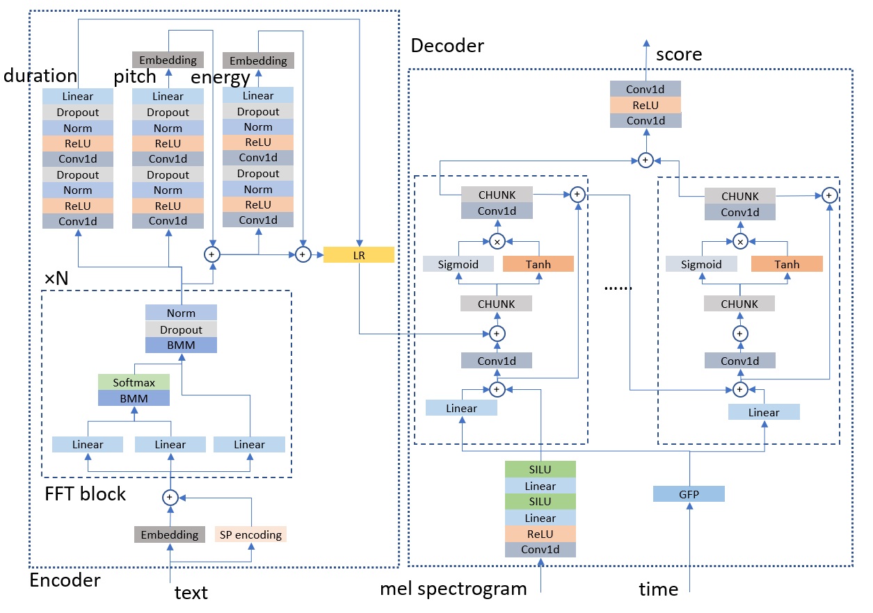
Figure 1: The architecture of ItôTTS.

ItôWave’s score prediction network structure $\mathfrak{S}_{\theta}(\mathbf{x}(t),t,\mathbf{m})$, as shown in Figure 2, is slightly simpler than $\mathfrak{S}_{\theta}(\mathbf{x}(t),t,\mathbf{p})$. The input is the wave to be generated, and the conditional input has mel spectrogram and time $t$. The output is the score at time $t$. All three types of input require preprocessing processes. The preprocessing of the wave is through a convolution layer; the preprocessing of mel spectrogram is based on the upsampling by two transposed convolution layers; and the preprocessing of step time $t$ is the same as in ItôTTS. After all inputs are preprocessed, they will be sent to the most critical module of $\mathfrak{S}_{\theta}(\mathbf{x}(t),t,\mathbf{m})$, which is very similar to the decoder of $\mathfrak{S}_{\theta}(\mathbf{x}(t),t,\mathbf{p})$ in ItôTTS, that is several serially connected dilated residual blocks. The main input of the dilated residual block is the wave, and the step time condition and mel spectrogram condition will be input into these dilated residual blocks one after another, and added to the feature map after the transformation of the wave signal. Similarly, there are two outputs of each dilated residual block, one is the state, which is used for input to the next residual block, and the other is the final output. The advantage of this is the ability to synthesize information of different granularities. Finally, the outputs of all residual blocks are summed and then pass through two convolution layers as the final output score.

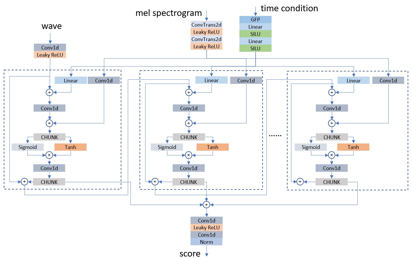
Figure 2: The architecture of ItôWave.

4 Experiments

4.1 Dataset and setup

The data set we use is LJSpeech [10], a single female speech database, with a total of 24 hours, 13100 sentences, randomly divided into 13000/50/50 for training/verification/testing. The sampling rate is 22050. In the experiment, all the places that involve mel spectrogram, whether it is in ItôTTS or in ItôWave, window length is 1024, hop length is 256, the number of mel channels is 80. We use the same Adam [13] training algorithm for ItôTTS and ItôWave. We have done quantitative evaluations based on mean opinion score (MOS) with other state-of-the-art methods on ItôTTS and ItôWave respectively. For ItôTTS, we compared with Tacotron 2 [28] and Fastspeech 2 [26], and for ItôWave, we compared with WaveNet [19], WaveGlow [24], Diffwave [14], and WaveGrad [3]. All experiments were performed on a GeForce RTX 3090 GPU with 24G memory.

4.2 Results and discussion

In order to verify the naturalness and fidelity of the synthesized voice, we randomly select 40 from 50 test data for each subject, and then let the subject give the synthesized sound a MOS score of 0-5.

In order to compare the synthesis quality of ItôTTS with Tacotron 2 [28] and Fastspeech 2 [26], a pre-trained HiFi-GAN model [32] as a vocoder to transform the mel spectrogram into a wave. In the experiment, ItôTTS uses 4 FFT layers in the encoder, three variance adaptors are used to predict the duration, pitch and energy of the phoneme respectively. 8 decoders, each of which is responsible for 10 channels of the mel spectrogram. Each decoder has 30 residual layers. The parameters of VE linear SDE in the experiment are $\sigma_{0}=0.01$, $\sigma_{1}=50$, and the number of time steps $N=1000$. The parameters of SDE used in ItôWave are the same.

In the structure of Tacotron 2 [28], there are 3 convolution layers in the encoder, the dimensions of recurrent neural network (RNN) and attention in the decoder are both 1024, and the postnet has 5 convolution layers. The batch size is 32. In the structure of Fastspeech 2 [26], the FFT block in the encoder has 4 layers, the FFT block in the decoder has 6 layers, and the dropout in both the encoder and the decoder is 0.2.

The results are shown in Table 1. MOS with 95% confidence is used in a comparative study of different state-of-the-art TTS systems on the test set of LJSpeech dataset. It can be seen that the MOS of ItôTTS is slightly better than the previous state-of-the-art method.

Table 1: MOS with 95% confidence in a comparative study of different state-of-the-art TTS methods on the test set of LJspeech dataset. All methods use a pre-trained HiFi-GAN model as the vocoder.

Methods	MOS
Ground truth	4.45$\pm$ 0.07
Tacotron 2	3.775$\pm$ 0.161
Fastspeech 2	3.9$\pm$ 0.159
ItôTTS	3.925$\pm$ 0.160

For the vocoder ItôWave, the original mel spectrogram of the test set was used as the condition input to the score estimation network. ItôWave uses 30 residual layers. For the comparison methods, WaveNet [19] uses 4 stacks with each stack consists of 24 dilated convolution layers. WaveGlow [24] uses 12 flows, and each flow uses an 8-layer wavenet to similarly make a reversible transform. Diffwave [14] uses a 30-layer dilated residual block, the number of reesidual channels is 64. WaveGrad [3] uses 5 layers of upsampling and 4 layers of downsampling.

The results are shown in Table 2, and you can see that ItôWave scores the best. It has approached the true value of ground truth.

Table 2: MOS with 95% confience in a comparative study of different state-of-the-art vocoders on the test set of LJspeech dataset.

Methods	MOS
Ground truth	4.45$\pm$ 0.07
WaveNet	4.3$\pm$ 0.130
WaveGlow	3.95$\pm$ 0.161
DiffWave	4.325$\pm$ 0.123
WaveGrad	4.1$\pm$ 0.158
ItôWave	4.35$\pm$ 0.115

5 Conclusion

This paper proposes ItôTTS and ItôWave, general methods based on linear SDE that can accomplish TTS and vocoder tasks at the same time. Under conditional input, ItôTTS and ItôWave can continuously transform simple distributions into corresponding mel spectrogram data or wave data through reverse-time linear SDE and Langevin dynamic. ItôTTS and ItôWave use neural networks to predict the required score for reverse-time linear SDE and Langevin dynamic sampling, which is the gradient of the log probability density at a specific time. For ItôTTS and ItôWave, we designed the corresponding effective score prediction networks. Experiments show that the MOS of ItôTTS and ItôWave can achieved the state-of-the-art respectively.

For future work, we believe that there are three important research directions. The first is to study different linear SDEs, that is, how different drift and diffusion coefficients affect the generation effect, and further, how to choose drift and diffusion coefficients to get the best Generation effect; in addition, study how to sample faster under the already trained score network, which is to speed up the generation speed; finally, extend this method to the generation of discrete data, such as the generation of midi music.

Appendix A Appendix

This appendix contains a lot of details that are not expanded in the text, including training algorithm of ItôWave’s score prediction network, ItôWave’s waveform generation algorithm, the influence of different numbers of decoders in ItôTTS, and examples of the generation process of mel spectrogram and wave in ItôTTS and ItôWave.

A.1 Algorithms

The training algorithms of the score network $\mathfrak{S}_{\theta}$ for ItôWave are shown in Algorithm 3 and Algorithm 4.

Algorithm 3 Training of the score network in general SDE-based wave generation model

Input and initialization: The audio wave $\mathbf{x}$ and the corresponding mel spectrograms $\mathbf{m}$, the diffusion time $T$.

1: for $k=0,1,\cdots$

2:  Uniformly sample $t$ from $[0,T]$.

3:   Randomly sample batch of $\mathbf{x}$ and $\mathbf{m}$, let $\mathbf{x}(0)=\mathbf{x}$, compute $\mathbf{x}(t)$ and $\nabla_{\mathbf{x}(t)}\log p(\mathbf{x}(t)|\mathbf{x}(0))$, then average the following

$$loss=\frac{1}{2}\parallel\mathfrak{S}_{\theta_{k}}(\mathbf{x}(t),t,\mathbf{m})-\nabla_{\mathbf{x}(t)}\log p(\mathbf{x}(t)|\mathbf{x}(0))\parallel^{2}.$$

4:   Do the back-propagation and the parameter updating of $\mathfrak{S}_{\theta}$.

5:  $k\leftarrow k+1$.

6: Until stopping conditions are satisfied and $\mathfrak{S}_{\theta_{k}}$ converges, e.g. to $\mathfrak{S}_{\theta_{*}}$.

Output: $\mathfrak{S}_{\theta_{*}}$.

Algorithm 4 Training of the score network in VE SDE-based wave generation model

Input and initialization: The audio wave $\mathbf{x}$ and the corresponding mel spectrograms $\mathbf{m}$, the diffusion time $T$.

1: for $k=0,1,\cdots$

2:  Uniformly sample $t$ from $[0,T]$.

3:   Randomly sample batch of $\mathbf{x}$ and $\mathbf{m}$, let $\mathbf{x}(0)=\mathbf{x}$. Sample $\mathbf{x}(t)$ from the distribution $\mathcal{N}\left(\mathbf{x}(t);\mathbf{x}(0),\left[\sigma_{0}^{2}(\frac{\sigma_{1}}{\sigma_{0}})^{2t}-\sigma_{0}^{2}\right]\mathbf{I}\right)$, compute the target score as $-\frac{\mathbf{x}(t)-\mathbf{x}(0)}{\sigma_{0}^{2}(\frac{\sigma_{1}}{\sigma_{0}})^{2t}-\sigma_{0}^{2}}$. Average the following

$$\text{DSM }loss=\parallel\mathfrak{S}_{\theta_{k}}(\mathbf{x}(t),t,\mathbf{m})+\frac{\mathbf{x}(t)-\mathbf{x}(0)}{\sigma_{0}^{2}(\frac{\sigma_{1}}{\sigma_{0}})^{2t}-\sigma_{0}^{2}}\parallel_{1}.$$

4:   Do the back-propagation and the parameter updating of $\mathfrak{S}_{\theta}$.

5:  $k\leftarrow k+1$.

6: Until stopping conditions are satisfied and $\mathfrak{S}_{\theta_{k}}$ converges, e.g. to $\mathfrak{S}_{\theta_{*}}$.

Output: $\mathfrak{S}_{\theta_{*}}$.

The wave generation algorithms of ItôWave are shown in Algorithm 5 and Algorithm 6.

Algorithm 5 General SDE-based ItôWave wave generation algorithm

Input and initialization: the score network $\mathfrak{S}_{\theta_{*}}$, input mel spectrogram $\mathbf{m}$, and $\mathbf{x}(N\Delta t)\sim\mathcal{N}\left(\mathbf{0},s\mathbf{I}\right)$.

1: for $k=N-1,\cdots,0$

2:  $\mathbf{x}(k\Delta t)=\mathbf{x}(k\Delta t+\Delta t)-\mathbf{f}(\mathbf{x}(k\Delta t+\Delta t),k\Delta t+\Delta t)\Delta t+g(k\Delta t+\Delta t)^{2}\mathfrak{S}_{\theta_{*}}(\mathbf{x}(k\Delta t+\Delta t),k\Delta t+\Delta t,\mathbf{m})\Delta t+g(k\Delta t+\Delta t)\mathbf{\xi}(k\Delta t)$

3:  $\mathbf{x}(k\Delta t)\leftarrow\mathbf{x}(k\Delta t)+\epsilon_{k}\mathfrak{S}_{\theta_{*}}(\mathbf{x}(k\Delta t),k\Delta t,\mathbf{m})+\sqrt{2\epsilon_{k}}\mathbf{\xi}(k\Delta t)$

4:  $k\leftarrow k-1$.

Output: The generated wave $\mathbf{x}(0)$.

Algorithm 6 VE SDE-based ItôWave wave generation algorithm

Input and initialization: the score network $\mathfrak{S}_{\theta_{*}}$, input mel spectrogram $\mathbf{m}$, and $\mathbf{x}(N\Delta t)\sim\mathcal{N}\left(\mathbf{0},s\mathbf{I}\right)$.

1: for $k=N-1,\cdots,0$

2:  $\mathbf{x}(k\Delta t)=\mathbf{x}(k\Delta t+\Delta t)+2\sigma_{0}^{2}(\frac{\sigma_{1}}{\sigma_{0}})^{2k\Delta t+2\Delta t}\log\frac{\sigma_{1}}{\sigma_{0}}\mathfrak{S}_{\theta_{*}}(\mathbf{x}(k\Delta t+\Delta t),k\Delta t+\Delta t,\mathbf{m})\Delta t+\sigma_{0}(\frac{\sigma_{1}}{\sigma_{0}})^{k\Delta t+\Delta t}\sqrt{2\log\frac{\sigma_{1}}{\sigma_{0}}}\mathbf{\xi}(k\Delta t)$

3:  $\mathbf{x}(k\Delta t)\leftarrow\mathbf{x}(k\Delta t)+\epsilon_{k}\mathfrak{S}_{\theta_{*}}(\mathbf{x}(k\Delta t),k\Delta t,\mathbf{m})+\sqrt{2\epsilon_{k}}\mathbf{\xi}(k\Delta t)$

4:  $k\leftarrow k-1$.

Output: The generated wave $\mathbf{x}(0)$.

A.2 Decoding multiple subbands of mel spectrogram separately in ItôTTS

As shown in the Figure 3 and Figure 4, if only one decoder is used for all the bands or channels of the mel spectrogram, the result is that the training cannot be achieved, and an interesting phenomenon is also found, that is, the network will first learn the easy-to-learn parts, such as the part without complex harmonics textures.

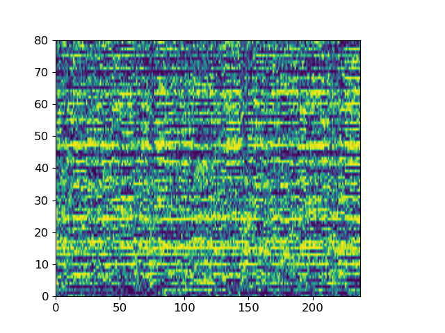
(a) Use the checkpoint obtained in the tenth epoch.

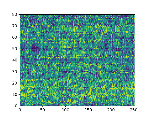
(b) In the 20th epoch.

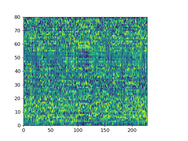
(c) In the 30th epoch.

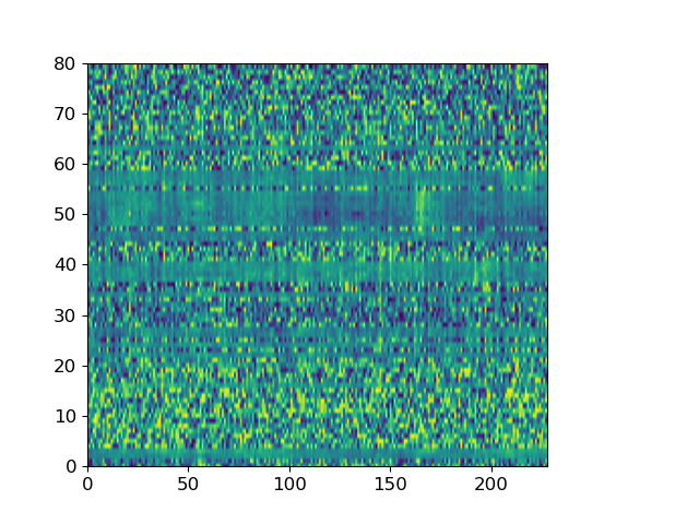
(d) In the 50th epoch.

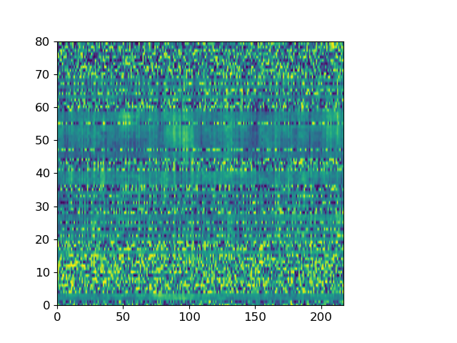
(e) In the 70th epoch.

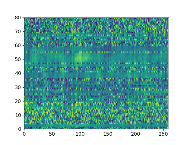
(f) In the 90th epoch.

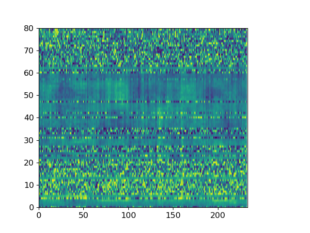
(g) In the 100th epoch.

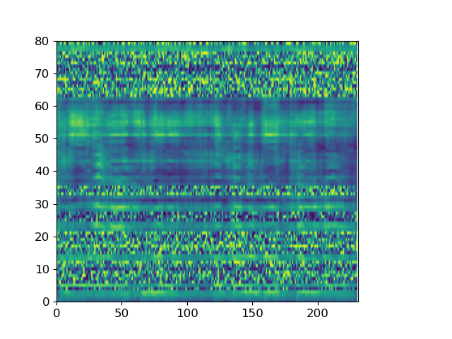
(h) In the 1000th epoch.

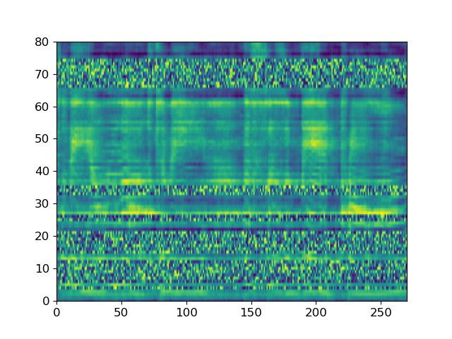
(i) In the 3000th epoch.

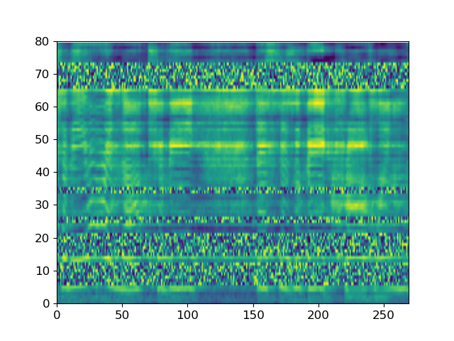
(j) In the 5000th epoch.

Figure 3: In ItôTTS, only one decoder is used to decode all 80 channels in the mel spectrogram, the checkpoints obtained during the training process is used to generate the mel spectrogram, conditioned on the text “to be or not to be, this is a big problem”.

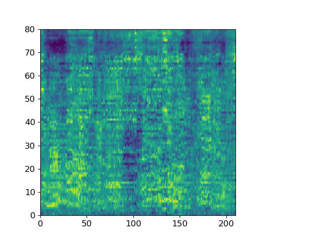
(a) Use the checkpoint obtained in the tenth epoch.

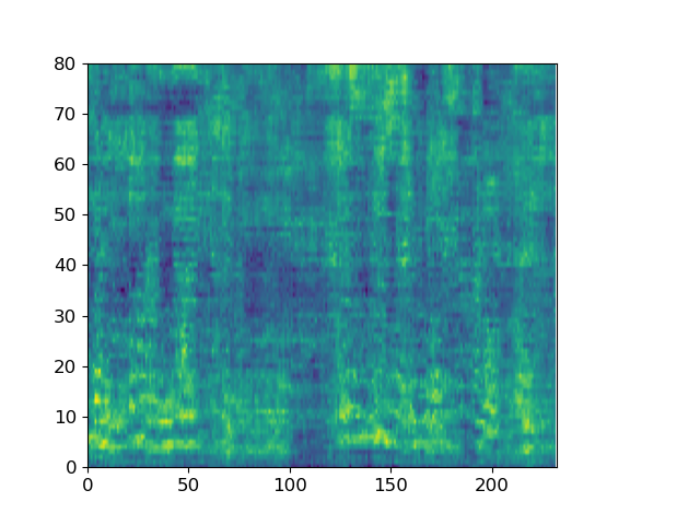
(b) In the 20th epoch.

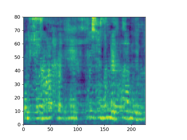
(c) In the 30th epoch.

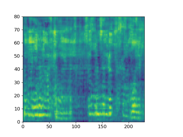
(d) In the 50th epoch.

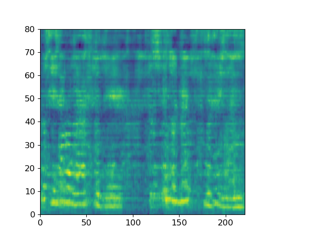
(e) In the 70th epoch.

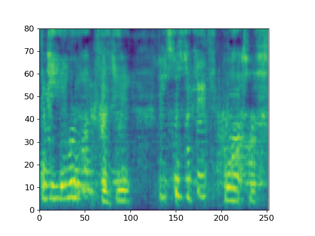
(f) In the 90th epoch.

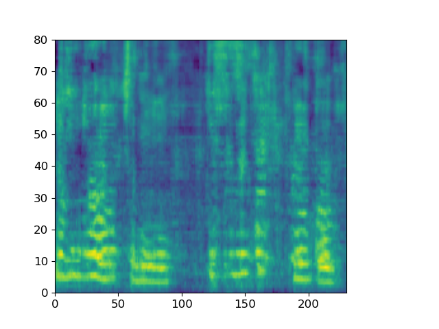
(g) In the 100th epoch.

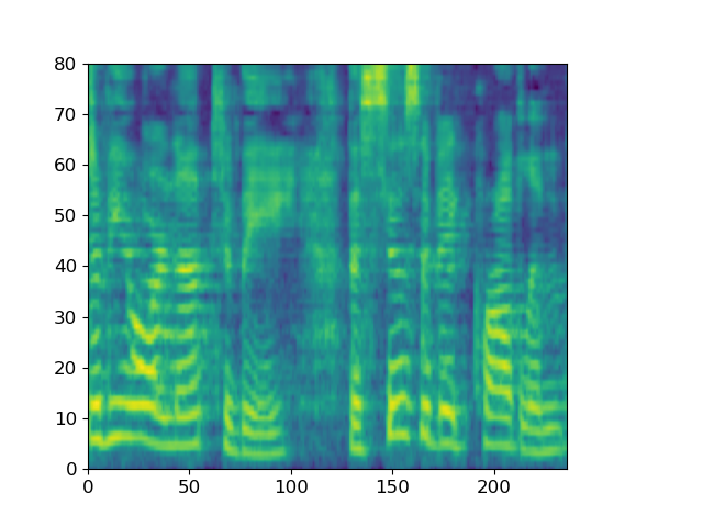
(h) In the 1000th epoch.

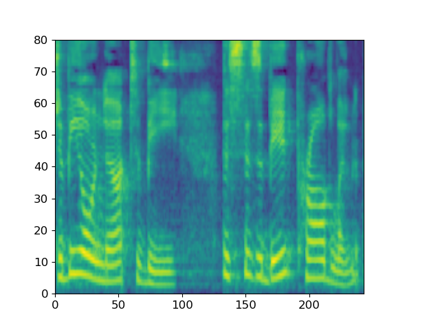
(i) In the 3000th epoch.

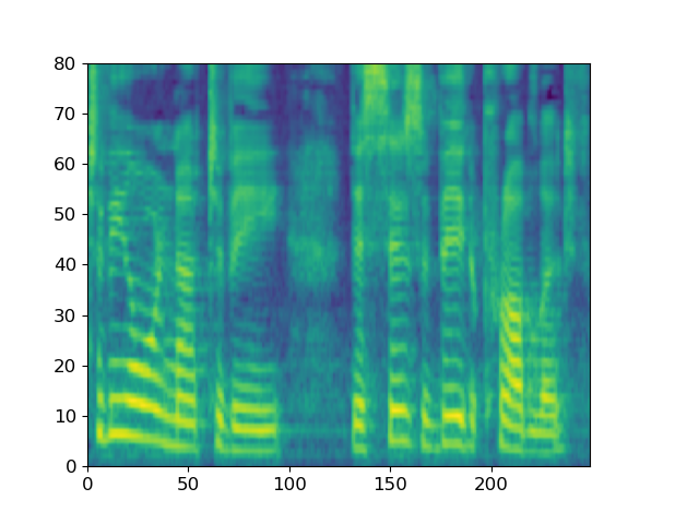
(j) In the 5000th epoch.

Figure 4: In ItôTTS, several decoders are used, each decoder is only responsible for decoding the limited channels in the mel spectrogram. For example, 8 decoders are used, and each is only responsible for decoding 10 channels, and the checkpoint obtained during the training process is used to generate the mel spectrogram, conditioned on the text “to be or not to be, this is a big problem”.

A.3 Diffusion generation of the mel spectrogram

As shown in the Figure 5, we can see how ItôTTS gradually turns white noise into mel spectrogram.

(a) Mel spectrogram in the first step.

(b) At the 200th step.

(c) At the 300th step.

(d) At the 400th step.

(e) At the 500th step.

(f) At the 600th step.

(g) At the 700th step.

(h) At the 800th step.

(i) At the 900th step.

(j) Mel spectrogram at the 1000th step.

Figure 5: Conditioned on the text “to be or not to be, this is a big problem”, ItôTTS gradually generates the corresponding mel spectrogram from the Gaussian signal step by step.

A.4 Diffusion generation of the wave

As shown in the Figure 6, we can see how ItôWave gradually turns white noise into meaningful wave.

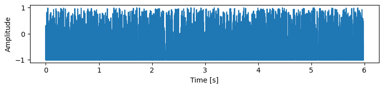
(a) The waveform in the first step.

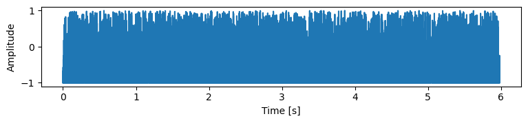
(b) The waveform at the 200th step.

(c) The waveform at the 300th step.

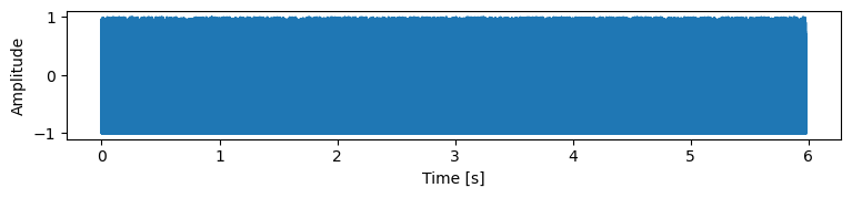
(d) The waveform at the 400th step.

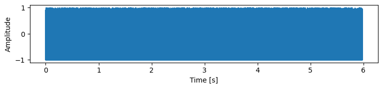
(e) The waveform at the 500th step.

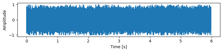
(f) The waveform at the 600th step.

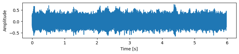
(g) The waveform at the 700th step.

(h) The waveform at the 800th step.

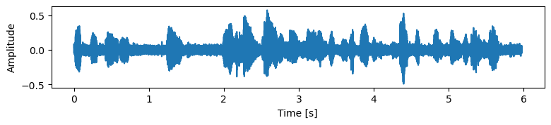
(i) The waveform at the 900th step.

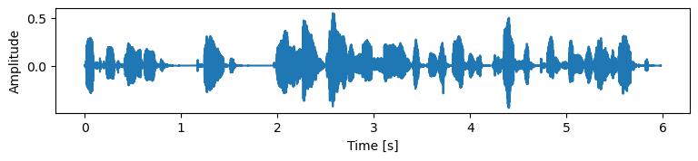
(j) The waveform at the 1000th step.

Figure 6: Conditioned on the frequency spectrum of the sentence LJ032-0167 in LJSpeech, ItôWave generates the corresponding voice step by step from the Gaussian signal. The corresponding text is “he concluded, quote, there is no doubt in my mind that these fibers could have come from this shirt.”

References

- Anderson [1982] Brian DO Anderson. Reverse-time diffusion equation models. Stochastic Processes and their Applications, 12(3):313–326, 1982.
- Bińkowski et al. [2019] Mikołaj Bińkowski, Jeff Donahue, Sander Dieleman, Aidan Clark, Erich Elsen, Norman Casagrande, Luis C Cobo, and Karen Simonyan. High fidelity speech synthesis with adversarial networks. arXiv preprint arXiv:1909.11646, 2019.
- Chen et al. [2020] Nanxin Chen, Yu Zhang, Heiga Zen, Ron J Weiss, Mohammad Norouzi, and William Chan. Wavegrad: Estimating gradients for waveform generation. arXiv preprint arXiv:2009.00713, 2020.
- Elfwing et al. [2018] Stefan Elfwing, Eiji Uchibe, and Kenji Doya. Sigmoid-weighted linear units for neural network function approximation in reinforcement learning. Neural Networks, 107:3–11, 2018.
- Engel et al. [2019] Jesse Engel, Kumar Krishna Agrawal, Shuo Chen, Ishaan Gulrajani, Chris Donahue, and Adam Roberts. Gansynth: Adversarial neural audio synthesis. arXiv preprint arXiv:1902.08710, 2019.
- Evans [2012] Lawrence C Evans. An introduction to stochastic differential equations, volume 82. American Mathematical Soc., 2012.
- Gibiansky et al. [2017] Andrew Gibiansky, Sercan Ömer Arik, Gregory Frederick Diamos, John Miller, Kainan Peng, Wei Ping, Jonathan Raiman, and Yanqi Zhou. Deep voice 2: Multi-speaker neural text-to-speech. In NIPS, 2017.
- Ho et al. [2020] Jonathan Ho, Ajay Jain, and Pieter Abbeel. Denoising diffusion probabilistic models. arXiv preprint arXiv:2006.11239, 2020.
- Hyvärinen and Dayan [2005] Aapo Hyvärinen and Peter Dayan. Estimation of non-normalized statistical models by score matching. Journal of Machine Learning Research, 6(4), 2005.
- Ito and Johnson [2017] Keith Ito and Linda Johnson. The lj speech dataset. Online: https://keithito. com/LJ-Speech-Dataset, 2017.
- Kim et al. [2018] Sungwon Kim, Sang-Gil Lee, Jongyoon Song, Jaehyeon Kim, and Sungroh Yoon. Flowavenet: A generative flow for raw audio. arXiv preprint arXiv:1811.02155, 2018.
- Kim et al. [2020] Jaehyeon Kim, Sungwon Kim, Jungil Kong, and Sungroh Yoon. Glow-tts: A generative flow for text-to-speech via monotonic alignment search. arXiv preprint arXiv:2005.11129, 2020.
- Kingma and Ba [2014] Diederik P Kingma and Jimmy Ba. Adam: A method for stochastic optimization. arXiv preprint arXiv:1412.6980, 2014.
- Kong et al. [2020] Zhifeng Kong, Wei Ping, Jiaji Huang, Kexin Zhao, and Bryan Catanzaro. Diffwave: A versatile diffusion model for audio synthesis. arXiv preprint arXiv:2009.09761, 2020.
- Kumar et al. [2019] Kundan Kumar, Rithesh Kumar, Thibault de Boissiere, Lucas Gestin, Wei Zhen Teoh, Jose Sotelo, Alexandre de Brébisson, Yoshua Bengio, and Aaron Courville. Melgan: Generative adversarial networks for conditional waveform synthesis. arXiv preprint arXiv:1910.06711, 2019.
- Liu et al. [2021] Peng Liu, Yuewen Cao, Songxiang Liu, Na Hu, Guangzhi Li, Chao Weng, and Dan Su. Vara-tts: Non-autoregressive text-to-speech synthesis based on very deep vae with residual attention. arXiv preprint arXiv:2102.06431, 2021.
- Mehri et al. [2016] Soroush Mehri, Kundan Kumar, Ishaan Gulrajani, Rithesh Kumar, Shubham Jain, Jose Sotelo, Aaron Courville, and Yoshua Bengio. Samplernn: An unconditional end-to-end neural audio generation model. arXiv preprint arXiv:1612.07837, 2016.
- Miao et al. [2020] Chenfeng Miao, Shuang Liang, Minchuan Chen, Jun Ma, Shaojun Wang, and Jing Xiao. Flow-tts: A non-autoregressive network for text to speech based on flow. In ICASSP 2020-2020 IEEE International Conference on Acoustics, Speech and Signal Processing (ICASSP), pages 7209–7213. IEEE, 2020.
- Oord et al. [2016] Aaron van den Oord, Sander Dieleman, Heiga Zen, Karen Simonyan, Oriol Vinyals, Alex Graves, Nal Kalchbrenner, Andrew Senior, and Koray Kavukcuoglu. Wavenet: A generative model for raw audio. arXiv preprint arXiv:1609.03499, 2016.
- Oord et al. [2018] Aaron Oord, Yazhe Li, Igor Babuschkin, Karen Simonyan, Oriol Vinyals, Koray Kavukcuoglu, George Driessche, Edward Lockhart, Luis Cobo, Florian Stimberg, et al. Parallel wavenet: Fast high-fidelity speech synthesis. In International conference on machine learning, pages 3918–3926. PMLR, 2018.
- Ping et al. [2018a] Wei Ping, Kainan Peng, and Jitong Chen. Clarinet: Parallel wave generation in end-to-end text-to-speech. arXiv preprint arXiv:1807.07281, 2018.
- Ping et al. [2018b] Wei Ping, Kainan Peng, Andrew Gibiansky, Sercan O Arik, Ajay Kannan, Sharan Narang, Jonathan Raiman, and John Miller. Deep voice 3: 2000-speaker neural text-to-speech. Proc. ICLR, pages 214–217, 2018.
- Popov et al. [2021] Vadim Popov, Ivan Vovk, Vladimir Gogoryan, Tasnima Sadekova, and Mikhail Kudinov. Grad-tts: A diffusion probabilistic model for text-to-speech. arXiv preprint arXiv:2105.06337, 2021.
- Prenger et al. [2019] Ryan Prenger, Rafael Valle, and Bryan Catanzaro. Waveglow: A flow-based generative network for speech synthesis. In ICASSP 2019-2019 IEEE International Conference on Acoustics, Speech and Signal Processing (ICASSP), pages 3617–3621. IEEE, 2019.
- Ren et al. [2019] Yi Ren, Yangjun Ruan, Xu Tan, Tao Qin, Sheng Zhao, Zhou Zhao, and Tie-Yan Liu. Fastspeech: Fast, robust and controllable text to speech. arXiv preprint arXiv:1905.09263, 2019.
- Ren et al. [2020] Yi Ren, Chenxu Hu, Xu Tan, Tao Qin, Sheng Zhao, Zhou Zhao, and Tie-Yan Liu. Fastspeech 2: Fast and high-quality end-to-end text to speech. arXiv preprint arXiv:2006.04558, 2020.
- Särkkä and Solin [2019] Simo Särkkä and Arno Solin. Applied stochastic differential equations, volume 10. Cambridge University Press, 2019.
- Shen et al. [2018] Jonathan Shen, Ruoming Pang, Ron J Weiss, Mike Schuster, Navdeep Jaitly, Zongheng Yang, Zhifeng Chen, Yu Zhang, Yuxuan Wang, Rj Skerrv-Ryan, et al. Natural tts synthesis by conditioning wavenet on mel spectrogram predictions. In 2018 IEEE International Conference on Acoustics, Speech and Signal Processing (ICASSP), pages 4779–4783. IEEE, 2018.
- Sohl-Dickstein et al. [2015] Jascha Sohl-Dickstein, Eric Weiss, Niru Maheswaranathan, and Surya Ganguli. Deep unsupervised learning using nonequilibrium thermodynamics. In International Conference on Machine Learning, pages 2256–2265. PMLR, 2015.
- Song and Ermon [2019] Yang Song and Stefano Ermon. Generative modeling by estimating gradients of the data distribution. arXiv preprint arXiv:1907.05600, 2019.
- Song et al. [2020] Yang Song, Jascha Sohl-Dickstein, Diederik P Kingma, Abhishek Kumar, Stefano Ermon, and Ben Poole. Score-based generative modeling through stochastic differential equations. arXiv preprint arXiv:2011.13456, 2020.
- Su et al. [2020] Jiaqi Su, Zeyu Jin, and Adam Finkelstein. Hifi-gan: High-fidelity denoising and dereverberation based on speech deep features in adversarial networks. arXiv preprint arXiv:2006.05694, 2020.
- Valin and Skoglund [2019] Jean-Marc Valin and Jan Skoglund. Lpcnet: Improving neural speech synthesis through linear prediction. In ICASSP 2019-2019 IEEE International Conference on Acoustics, Speech and Signal Processing (ICASSP), pages 5891–5895. IEEE, 2019.
- Valle et al. [2020] Rafael Valle, Kevin Shih, Ryan Prenger, and Bryan Catanzaro. Flowtron: an autoregressive flow-based generative network for text-to-speech synthesis. arXiv preprint arXiv:2005.05957, 2020.
- Vincent [2011] Pascal Vincent. A connection between score matching and denoising autoencoders. Neural computation, 23(7):1661–1674, 2011.
- Wang et al. [2017] Yuxuan Wang, RJ Skerry-Ryan, Daisy Stanton, Yonghui Wu, Ron J Weiss, Navdeep Jaitly, Zongheng Yang, Ying Xiao, Zhifeng Chen, Samy Bengio, et al. Tacotron: Towards end-to-end speech synthesis. arXiv preprint arXiv:1703.10135, 2017.
- Yamamoto et al. [2020] Ryuichi Yamamoto, Eunwoo Song, and Jae-Min Kim. Parallel wavegan: A fast waveform generation model based on generative adversarial networks with multi-resolution spectrogram. In ICASSP 2020-2020 IEEE International Conference on Acoustics, Speech and Signal Processing (ICASSP), pages 6199–6203. IEEE, 2020.