T2-DAG: a powerful test for differentially expressed gene pathways via graph-informed structural equation modeling

Abstract

Motivation: A major task in genetic studies is to identify genes related to human diseases and traits to understand functional characteristics of genetic mutations and enhance patient diagnosis. Compared to marginal analyses of individual genes, identification of gene pathways, i.e., a set of genes with known interactions that collectively contribute to specific biological functions, can provide more biologically meaningful results. Such gene pathway analysis can be formulated into a high-dimensional two-sample testing problem. Given the typically limited sample size of gene expression datasets, most existing two-sample tests tend to have compromised powers because they ignore or only inefficiently incorporate the auxiliary pathway information on gene interactions.
Results: We propose T2-DAG, a Hotelling’s $T^{2}$-type test for detecting differentially expressed gene pathways, which efficiently leverages the auxiliary pathway information on gene interactions from existing pathway databases through a linear structural equation model. We further establish its asymptotic distribution under pertinent assumptions. Simulation studies under various scenarios show that T2-DAG outperforms several representative existing methods with well-controlled type-I error rates and substantially improved powers, even with incomplete or inaccurate pathway information or unadjusted confounding effects. We also illustrate the performance of T2-DAG in an application to detect differentially expressed KEGG pathways between different stages of lung cancer.
Availability: The R package T2DAG is available on Github at https://github.com/Jin93/T2DAG.
Contact: jjin31@jhu.edu; yue.wang.stat@asu.edu
Supplementary information: Supplementary data are available at Bioinformatics online.

1 Introduction

With the continuous development of high-throughput sequencing technologies, there is an increasing need for powerful statistical methods for large-scale quantitative comparison between populations/conditions. For example, in gene expression data analysis, a major task is to identify genes from a large gene list that express differentially between different conditions, such as different disease statuses. Various approaches have been proposed for this task, providing critical insights into the molecular basis of many complex human traits/diseases; see Robinson et al. (2010), Love et al. (2014) and the references therein.

Besides separately analyzing individual genes, recently there is a growing interest in detecting differentially expressed gene pathways. Here, a gene pathway refers to a set of correlated genes with known interactions collectively contributing to specific biological functions. Many biologically meaningful gene pathways have been identified via experiments or statistical modeling, along with identified gene interactions, such as activation/expression or inhibition/repression of one gene by another. Public databases containing such pathways include Kyoto Encyclopedia of Genes and Genomes (KEGG, Kanehisa and Goto, 2000; Kanehisa et al., 2019), Gene Ontology (GO, Ashburner et al., 2000; Consortium, 2019), BioCarta databases (Nishimura, 2001), etc. Fig. 1 shows two directed acyclic graphs (DAGs) illustrating two KEGG gene pathways, which will be revisited in our data analysis in Section 4. $a$ $b$ and $a$ $b$ both indicate activation from gene $a$ to gene $b$; $a\dashrightarrow b$ and $a$ $b$ indicate expression and inhibition, respectively, from gene $a$ to gene $b$. A common and notable feature of the two pathways is the high sparsity of the edges in the corresponding DAGs; that is, only a small proportion of the gene pairs are connected. Such sparsity pattern is also present in most identified gene pathways (Wille et al., 2004; Li et al., 2012; Chun et al., 2015).

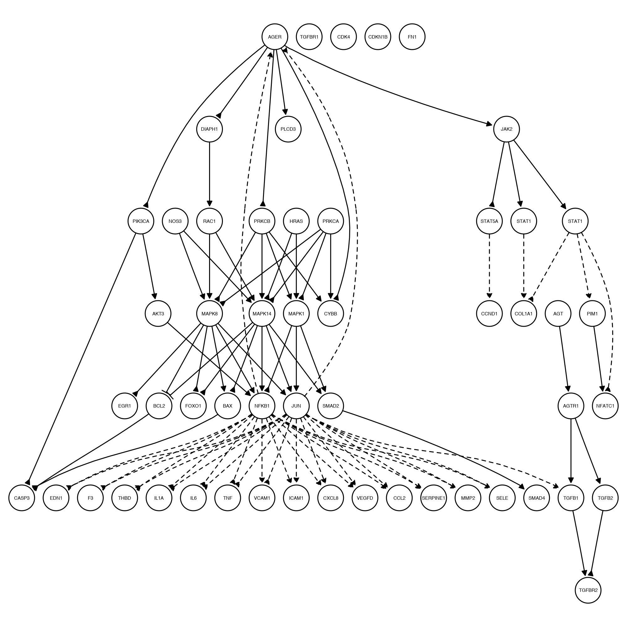
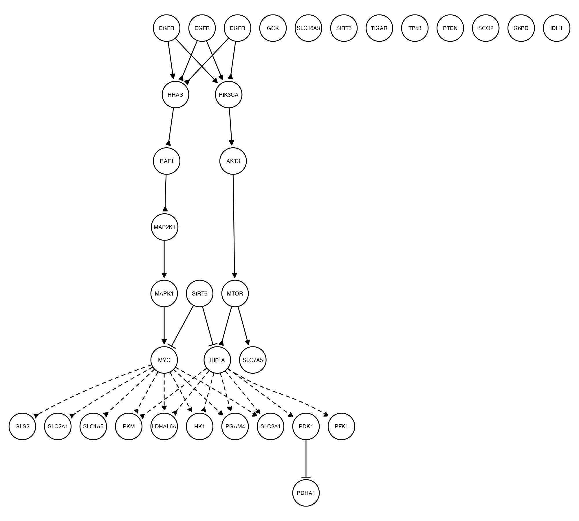
Figure 1: Directed acyclic graphs (DAGs) describing gene interactions in an AGE-RAGE signaling pathway in diabetic complications (left panel) and a pathway for central carbon metabolism in cancer (right panel) from the KEGG database.

There are two main reasons for investigating differentially expressed gene pathways over individual genes. First, marginal tests for individual genes tend to have low statistical power due to limited sample sizes of typical gene expression datasets. On the other hand, gene pathway tests can achieve enhanced power by aggregating concerted signals from multiple related genes in the same pathway. Second, marginal analyses of individual genes often ignore interactions among genes, which potentially lead to spurious conclusions inconsistent with the underlying biological processes. Since gene interactions can provide critical insights into the molecular mechanism of the progression of traits/diseases, efficiently leveraging the auxiliary information on gene interactions can facilitate the detection of disease- and trait-specific genes and yield biologically more meaningful results.

To formalize the problem, let $\mathcal{G}=(\mathcal{V},\mathcal{D})$ denote the pathway of interest, where $\mathcal{V}=\{1,\ldots,p\}$ and $\mathcal{D}$ denote the gene set and edge set between genes, respectively. We assume that $\mathcal{G}$ is a DAG; i.e., all edges in $\mathcal{D}$ are directed edges with no loops. A DAG $\mathcal{G}$ can be summarized by an adjacency matrix $A=(a_{jk})\in\mathbb{R}^{p\times p}$, where $a_{jk}=1$ if the edge $j\rightarrow k$ is present in $\mathcal{D}$, in which case we call gene $j$ a parent of gene $k$ and gene $k$ a child of gene $j$, and $a_{jk}=0$ otherwise. Although some identified gene pathways cannot be described by DAGs, they tend to have a small number of loops and/or undirected edges (see Table S1 for a summary of the KEGG pathways included in our data analysis). Thus, for such gene pathways, analyses based on their largest directed acyclic subgraphs are still feasible and informative. Approaches to directly handling non-DAG pathways are feasible but will require techniques different from the ones in this study, which we will briefly discuss in Section 5.

Assume we have observed expression levels of the genes in $\mathcal{V}$ for individuals in two different conditions. Specifically, let $x^{(l)}_{ij}$ denote the expression level of gene $j\in\mathcal{V}$ for individual $i\in\{1,\ldots,n_{l}\}$ in group $l\in\{1,2\}$. We assume that the data are appropriately transformed so that ${\bf x}^{(l)}_{i}=(x^{(l)}_{i1},\ldots,x^{(l)}_{ip})^{\intercal}$, $i=1,\ldots,n_{l}$, are independent and identically distributed (i.i.d.) random vectors from a multivariate Gaussian distribution with mean ${\mbox{\boldmath${\mu}$}}_{l}$ ($l=1,2$) and covariance $\Sigma$. Besides observed gene expression data, there is auxiliary information on the presence/absence of directed relationships among genes (contained in $\mathcal{D}$), such as activation/inhibition of one gene by another. Our goal is then to test for the inequality of the two population mean, i.e., $H_{0}\mathrel{\mathop{\mathchar 58\relax}}{\mbox{\boldmath${\mu}$}}_{1}={\mbox{\boldmath${\mu}$}}_{2}\text{ versus }H_{a}\mathrel{\mathop{\mathchar 58\relax}}{\mbox{\boldmath${\mu}$}}_{1}\neq{\mbox{\boldmath${\mu}$}}_{2}$, based on ${\bf x}^{(l)}_{i}$s, while efficiently leveraging the auxiliary information on gene interactions.

Conventional hypothesis testing for the inequality of two mean vectors has been thoroughly investigated. A classical approach is the Hotelling’s $T^{2}$ test (Hotelling, 1931) with the test statistic

$$T^{2}=\frac{n_{1}n_{2}}{n_{1}+n_{2}}(\overline{\bf x}^{(1)}-\overline{\bf x}^{(2)})^{\intercal}\widehat{\Sigma}^{-1}(\overline{\bf x}^{(1)}-\overline{\bf x}^{(2)}),$$ (1)

where $\overline{\bf x}^{(l)}=n_{l}^{-1}\sum_{i=1}^{n_{l}}{\bf x}^{(l)}_{i}$ and $\widehat{\Sigma}=(n_{1}+n_{2}-1)^{-1}\sum_{l=1}^{2}\sum_{i=1}^{n_{l}}({\bf x}^{(l)}_{i}-\overline{\bf x}^{(l)})({\bf x}^{(l)}_{i}-\overline{\bf x}^{(l)})^{\intercal}.$ When the number of genes $(p)$ is smaller than the total sample size $(n_{1}+n_{2})$, $T^{2}$ is well-defined; under $H_{0}$, $T^{2}\left(n_{1}+n_{2}-p-1\right)/\left(p\left(n_{1}+n_{2}-2\right)\right)$ follows an $F$-distribution with parameters $p$ and $n_{1}+n_{2}-1-p$. The $T^{2}$ is a sum-of-squares type of statistic powerful against “dense alternatives", where the signals of differential expression are scattered among a large number of genes. This can often be true for gene pathway analyses, as genes in the same pathway tend to have concerted signals of expression that together form certain biological functions.

While Hotelling’s $T^{2}$ is well known as the uniformly most powerful invariant (UMPI) test, it is not applicable when $p$ is larger than $(n_{1}+n_{2})$, referred to as the high-dimensional setting hereafter. This is simply because in the high-dimensional setting the sample covariance matrix $\widehat{\Sigma}$ becomes singular, making $T^{2}$ ill-posed. Research has been conducted extensively on extending $T^{2}$ to the high-dimensional setting. For example, Bai and Saranadasa (1996) and Srivastava and Du (2008) directly modified the ill-posed $T^{2}$ by replacing $\widehat{\Sigma}$ in (1) with the identity matrix $I$ and the diagonal of $\widehat{\Sigma}$, respectively. Lopes et al. (2011) proposed to first project the high-dimensional data onto a randomly constructed low-dimensional space and then perform the Hotelling’s $T^{2}$ test. Chen et al. (2011) replaced $\widehat{\Sigma}$ with $(\widehat{\Sigma}+\lambda I)$ for some regularization parameter $\lambda>0$ and proposed a nonparametric testing procedure. Recently, Li et al. (2020) extended the work of Chen et al. (2011) and proposed an Adaptive Regularized Hotelling’s $T^{2}$ (ARHT) test that combines the test statistics corresponding to a set of $\lambda$s optimally chosen by a data-adaptive selection mechanism. Methods that are not direct modifications of Hotelling’s $T^{2}$ are also extensive. For example, Cai et al. (2014) proposed the CLX test with a supremum-type test statistic powerful against “sparse” alternatives. Gregory et al. (2015) proposed the GCT test that avoids the estimation of $\widehat{\Sigma}^{-1}$ by assuming an ordering of the variables so that the dependence between variables can be modeled according to their displacement. Xu et al. (2016) proposed the aSPU test, a robust adaptive test powerful against a wide range of alternatives.

While these existing methods can, to varying degrees, handle potentially high-dimensional gene expression data, they cannot incorporate the auxiliary information on gene interactions available from pathway databases. Incorporating such auxiliary information could substantially improve the test power, especially considering the inadequate sample size of a typical gene expression dataset. Previous efforts to address this issue include the NetGSA test (Shojaie and Michailidis, 2009 and Shojaie and Michailidis, 2010), which assumes that the magnitude of gene interactions is priorly known and incorporates such information using a linear mixed model. This approach has limited applicability in real applications because the magnitude of gene interactions is often unknown or only partially known and needs to be estimated using external data. Another approach proposed by Jacob et al. (2012), referred to as the Graph T2 test hereafter, projects data onto a low-dimensional space spanned by top eigenvectors of the graph Laplacian of the gene pathway and then performs the dimension reduction test in Lopes et al. (2011). Unlike the NetGSA test, Graph T2 can simply incorporate information on the presence/absence of gene interactions, but it may have compromised power if the signal is not coherent with the selected eigenvectors of the corresponding graph Laplacian.

To address these limitations of the existing methods, we propose T2-DAG, a novel test for identifying differentially expressed gene pathways, which efficiently leverages auxiliary information on gene interactions. Unlike the NetGSA test that requires additional information on the magnitude of gene interactions, the T2-DAG test only requires information on the presence/absence of gene interactions, which is more easily accessible in practice. Although the Gragh T2 test also requires only the information on the presence/absence of gene interactions, it simply incorporates a few eigenvectors of the corresponding graph Laplacian. On the contrary, T2-DAG directly incorporates all gene interactions into the analysis with minimal information loss. Our main idea is to link the auxiliary information on gene interactions with (partial) correlations among genes through a linear structural equation model (SEM). Based on the SEM, we construct a novel pathway-informed estimator of the precision matrix of the genes via the LDL decomposition (Krishnamoorthy and Menon, 2013), where the ordering of the genes is naturally determined by the topological ordering of the pathway. We then construct a test statistic by replacing the ill-posed $\widehat{\Sigma}^{-1}$ in (1) with the novel estimator of the precision matrix followed by a $Z$-transformation, which is denoted by T2-DAG $Z$. Under mild conditions, we prove that the proposed test statistic converges in distribution to the standard normal distribution. An alternative T2-DAG $\chi^{2}$ test can be constructed without the $Z$-transformation, which converges in distribution to $\chi^{2}_{p}$ under more stringent conditions. We also derive the asymptotic power of the tests under local alternatives that characterize the true signals of differential expression in the gene pathway between two populations/conditions. Under various simulated data scenarios, the proposed T2-DAG tests show well-controlled type I error rates and substantially higher powers compared to multiple existing methods, even with partially missing or incorrect information on gene interactions, unadjusted confounding effects, or non-Gaussian error terms. Although theoretically limited, the T2-DAG $\chi^{2}$ test compares favorably to the T2-DAG $Z$ test in the simulated scenarios, where it has slightly higher but still well-controlled type I error rates and higher powers. We also demonstrate the efficiency of the T2-DAG tests in a lung cancer-related application to detect differentially expressed gene pathways between different cancer stages.

2 Methods

Recall that our goal is to test for inequality of the mean expression levels of a gene pathway in two populations, $H_{0}\mathrel{\mathop{\mathchar 58\relax}}{\mbox{\boldmath${\mu}$}}_{1}={\mbox{\boldmath${\mu}$}}_{2}\text{ versus }H_{a}\mathrel{\mathop{\mathchar 58\relax}}{\mbox{\boldmath${\mu}$}}_{1}\neq{\mbox{\boldmath${\mu}$}}_{2}$, based on observed gene expression data, ${\bf x}^{(l)}_{i}=(x^{(l)}_{i1},\ldots,x^{(l)}_{ip})^{\intercal}$, $i=1,\ldots,n_{l}$, $l=1,2$, while leveraging available auxiliary information on gene interactions described by a DAG $\mathcal{G}=(\mathcal{V},\mathcal{D})$. Throughout the article, we use $\xi_{1}\mathchoice{\mathrel{\hbox to0.0pt{$\displaystyle\perp$\hss}\mkern 2.0mu{\displaystyle\perp}}}{\mathrel{\hbox to0.0pt{$\textstyle\perp$\hss}\mkern 2.0mu{\textstyle\perp}}}{\mathrel{\hbox to0.0pt{$\scriptstyle\perp$\hss}\mkern 2.0mu{\scriptstyle\perp}}}{\mathrel{\hbox to0.0pt{$\scriptscriptstyle\perp$\hss}\mkern 2.0mu{\scriptscriptstyle\perp}}}\xi_{2}$ to denote the independence between two random variables $\xi_{1}$ and $\xi_{2}$. We write $g(n)=O(f(n))$ if and only if $\lim_{n\rightarrow\infty}g(n)/f(n)<\infty$, and use $g(n)=o(f(n))$ to denote $\lim_{n\rightarrow\infty}g(n)/f(n)=0$. We also write $f(n)\asymp g(n)$ if and only if $\lim_{n\rightarrow\infty}|f(n)/g(n)|=C$ for some constant $C>0$. Let $I(\mathcal{A})$ denote the indicator function of the event $\mathcal{A}$; i.e., $I(\mathcal{A})=1$ if $\mathcal{A}$ is true, and $I(\mathcal{A})=0$ otherwise. We use lowercase letters, bold lowercase letters, and uppercase letters to denote scalars, vectors, and matrices, respectively.

We first define a new random variable, ${\bf z}_{i}=(z_{i1},\ldots,z_{ip})^{\intercal}$, based on the original gene expression data, ${\bf x}^{(l)}_{i}$, $i=1,\ldots,n_{l}$, $l=1,2$:

$${\bf z}_{i}=\begin{cases}{\bf x}^{(1)}_{i}-{\mbox{\boldmath${\mu}$}}_{1}&i=1,2,\ldots,n_{1}\\ {\bf x}^{(2)}_{i-n_{1}}-{\mbox{\boldmath${\mu}$}}_{2}&i=n_{1}+1,\ldots,n_{1}+n_{2}.\end{cases}$$

Given that ${\bf x}^{(l)}_{i}$ are i.i.d. random vectors that follow a multivariate normal distribution $\mathcal{N}({\mbox{\boldmath${\mu}$}}_{l},\Sigma)$, we can easily check that ${\bf z}_{i}\stackrel{{\scriptstyle i.i.d.}}{{\sim}}\mathcal{N}({\mbox{\boldmath${0}$}},\Sigma)$, $i=1,2,\ldots,n_{1}+n_{2}$. We propose to model each ${\bf z}_{i}$ through the following SEM with a vector of Gaussian noises:

$${\bf z}_{i}=Q^{\intercal}{\bf z}_{i}+{\mbox{\boldmath${\epsilon}$}}_{i},$$ (2)

where $Q=(q_{jk})\in\mathbb{R}^{p\times p}$ is an unknown coefficient matrix with $q_{jk}$ characterizing the magnitude of the effect of gene $j$ on gene $k$, and ${\mbox{\boldmath${\epsilon}$}}_{i}=(\epsilon_{i1},\ldots,\epsilon_{ip})^{\intercal}$ are $i.i.d.$ random vectors following $\mathcal{N}({\mbox{\boldmath${0}$}},R)$. We make the following assumption on $R$:

Assumption 1.

$R=\text{diag}(r_{1},\ldots,r_{p})$.

Assumption 1 states that $\epsilon_{ij_{1}}\mathchoice{\mathrel{\hbox to0.0pt{$\displaystyle\perp$\hss}\mkern 2.0mu{\displaystyle\perp}}}{\mathrel{\hbox to0.0pt{$\textstyle\perp$\hss}\mkern 2.0mu{\textstyle\perp}}}{\mathrel{\hbox to0.0pt{$\scriptstyle\perp$\hss}\mkern 2.0mu{\scriptstyle\perp}}}{\mathrel{\hbox to0.0pt{$\scriptscriptstyle\perp$\hss}\mkern 2.0mu{\scriptscriptstyle\perp}}}\epsilon_{ij_{2}}$ for all $j_{1}\neq j_{2}$ and $i=1,\ldots,n_{1}+n_{2}$. This amounts to the assumption that there is no latent confounders, which is common in the existing SEM literature; see Loh and Bühlmann (2014), Peters and Bühlmann (2014), and the references therein. We next link the coefficient matrix $Q$ in model (2) with the DAG $\mathcal{G}$ through the following assumption.

Assumption 2.

The support of $Q$, i.e., the indices of nonzero entries in $Q$, is informed by $\mathcal{G}$ through the corresponding adjacency matrix $A=(a_{jk})$, such that $q_{jk}\neq 0$ if and only if $a_{jk}\neq 0$.

Assumption 2 is only required for theoretical analysis. Simulation studies in Section 3 will allow the auxiliary DAG to have missing or mis-specified edges. Since $\mathcal{G}$ is a DAG, we can label the variables in $\mathcal{V}$ according to the topological ordering of $\mathcal{G}$ so that $Q$ is a strictly upper triangular matrix, i.e., an upper triangular matrix with the diagonal entries being 0 (Loh and Bühlmann, 2014). As a result, model (2) can be rewritten as the following $p$ linear models:

$$z_{ij}=f_{j}(\epsilon_{i1},\ldots,\epsilon_{ij})\mbox{, }j=1,\ldots,p\mbox{, }i=1,\ldots,n_{1}+n_{2},$$

where $\{f_{j}(\cdot)\}_{j=1}^{p}$ are linear functions that are determined by $Q$. Thus, for $1\leq j_{2}<j_{1}\leq p$ and each $i$, one can check that $\mbox{Cov}(\epsilon_{ij_{1}},z_{ij_{2}})=0$, indicating that $\epsilon_{ij_{1}}\mathchoice{\mathrel{\hbox to0.0pt{$\displaystyle\perp$\hss}\mkern 2.0mu{\displaystyle\perp}}}{\mathrel{\hbox to0.0pt{$\textstyle\perp$\hss}\mkern 2.0mu{\textstyle\perp}}}{\mathrel{\hbox to0.0pt{$\scriptstyle\perp$\hss}\mkern 2.0mu{\scriptstyle\perp}}}{\mathrel{\hbox to0.0pt{$\scriptscriptstyle\perp$\hss}\mkern 2.0mu{\scriptscriptstyle\perp}}}z_{ij_{2}}$ under Gaussianity. This property will play an important role in establishing the asymptotic null distribution of our test statistic.

We next construct DAG-informed estimators of $\Sigma$ and $\Sigma^{-1}$. From model (2), we can obtain ${\mbox{\boldmath${\epsilon}$}}_{i}=(I-Q^{\intercal}){\bf z}_{i}$, $i=1,\ldots,n_{1}+n_{2}$. Applying the covariance function to both sides of this equation yields $R=(I-Q^{\intercal})\Sigma(I-Q).$ Since $Q$ is strictly upper triangular, we know that $I-Q$ is invertible, leading to

$$\Sigma=(I-Q^{\intercal})^{-1}R(I-Q)^{-1}.$$ (3)

Taking the inverse of both sides of (3) gives

$$\Sigma^{-1}=(I-Q){R}^{-1}(I-Q)^{\intercal}.$$ (4)

Equations (3) and (4) serve as the basis for the construction of the DAG-informed estimators of $\Sigma$ and $\Sigma^{-1}$, which are critical to the proposed test statistic. Note that (3) and (4) are, respectively, LDL-type decompositions of $\Sigma$ and $\Sigma^{-1}$; similar decompositions have been employed in the literature for estimating high-dimensional covariance/precision matrices (Wu and Pourahmadi, 2003; Huang et al., 2006). The rationale behind the LDL decomposition is that there exists some natural ordering of the variables, which, in the case of gene pathways, is determined by the topological ordering of the corresponding graph $\mathcal{G}$.

We observe from equations (3) and (4) that $\Sigma$ and $\Sigma^{-1}$ are functions of $Q$ and $R$. We then construct estimators for $Q$ and $R$. Letting ${\bf q}_{j}$ denote the $j$-th column of $Q$, we decompose model (2) into $p$ sub-models,

$$z_{ij}={\bf z}_{i}^{\intercal}{\bf q}_{j}+\epsilon_{ij},\mbox{ }j=1,\ldots,p.$$ (5)

To estimate the unknown parameters in (5), it is natural to consider the following square loss function for each sub-model $j$:

$$~{}\sum_{l=1}^{2}\sum_{i=1}^{n_{l}}\left\{x^{(l)}_{ij}-\mu_{lj}-\left({\bf x}^{(l)}_{i}-{{\mbox{\boldmath${\mu}$}}}_{l}\right)^{\intercal}{\bf q}_{j}\right\}^{2}$$

$$= ~{}\sum_{l=1}^{2}\sum_{i=1}^{n_{l}}\left\{x^{(l)}_{ij}-\gamma_{lj}-{\bf x}^{(l)\intercal}_{i}{\bf q}_{j}\right\}^{2},$$ (6)

where $\gamma_{lj}=\mu_{lj}+{{\mbox{\boldmath${\mu}$}}}_{l}^{\intercal}{\bf q}_{j}$. Letting $S_{j}=\{k\mathrel{\mathop{\mathchar 58\relax}}a_{kj}=1\}$, one can see that under Assumption 2, ${\bf q}_{j}$ has $|S_{j}|$ nonzero entries with $|S_{j}|\leq j-1$ for $j>1$ and that ${\bf q}_{1}={{\mbox{\boldmath${0}$}}}$. Since real gene pathways are far less dense than fully connected networks (Wille et al., 2004; Li et al., 2012; Chun et al., 2015), we make the following assumption on $S_{j}$:

Assumption 3.

$d=o(n_{1}+n_{2})$ as $n_{1},n_{2}\rightarrow\infty$, where $d=\max_{j}|S_{j}|$.

This assumption appears to be reasonable for all 206 pathways considered in our data analysis in Section 4 (see Table S1 for details). Under Assumptions 1-3, we can estimate $\gamma_{lj}$ and the nonzeros entries of ${\bf q}_{j}$ in (2) using the ordinary least squares (OLS). Specifically, denote by ${\bf 1}_{n_{1}+n_{2}}$ the $(n_{1}+n_{2})$-dimensional vector of all ones and let ${\bf g}=(g_{1},\ldots,g_{n_{1}+n_{2}})^{\intercal}$ denote the group indicator; that is, $g_{i}$ equals 1 for $i=1,\ldots,n_{1}$ and equals 0 for $i=n_{1}+1,\ldots,n_{1}+n_{2}$. Then, letting $X=\left[{\bf x}_{1}^{(1)}~{}\cdots~{}{\bf x}_{n_{1}}^{(1)}~{}{\bf x}_{1}^{(2)}~{}\cdots~{}{\bf x}_{n_{2}}^{(2)}\right]^{\intercal}$, we rewrite (2) in the following matrix form

$$\left\|X_{j}-\theta_{1j}{\bf 1}_{n_{1}+n_{2}}-\theta_{2j}{\bf g}-X_{S_{j}}{\bf q}_{j,S_{j}}\right\|_{2}^{2},$$ (7)

where $X_{j}$ denotes the $j$-th column of $X$, $X_{S_{j}}$ denotes the sub-matrix of $X$ with columns indexed by $S_{j}$, and ${\bf q}_{j,S_{j}}$ denotes the sub-vector of ${\bf q}_{j}$ with entries indexed by $S_{j}$ that are non-zero according to the DAG and need to be estimated. Comparing (7) with (2), one can see that $\gamma_{1j}=\theta_{1j}+\theta_{2j}$ and $\gamma_{2j}=\theta_{1j}$. Thus, letting $W=[{\bf 1}_{n_{1}+n_{2}}~{}{\bf g}]$, we can obtain the OLS estimator of ${\bf q}_{j,S_{j}}$ and $(\theta_{1j},\theta_{2j})^{\intercal}$:

$$\widehat{\bf q}_{j,S_{j}}= ~{}\left(X_{S_{j}}^{\intercal}(I_{n_{1}+n_{2}}-\mathcal{P}_{W})X_{S_{j}}\right)^{-1}X_{S_{j}}^{\intercal}(I_{n_{1}+n_{2}}-\mathcal{P}_{W})X_{j},$$

$$(\widehat{\theta}_{1j},\widehat{\theta}_{2j})^{\intercal}= ~{}(W^{\intercal}W)^{-1}W^{\intercal}\left(X_{j}-X_{S_{j}}\widehat{\bf q}_{j,S_{j}}\right),$$ (8)

where $\mathcal{P}_{W}=W(W^{\intercal}W)^{-1}W^{\intercal}$ is the orthogonal projection matrix onto the column space of $W$. For ease of notation, we also denote the OLS estimator of $q_{kj}$ by $\widehat{q}_{kj}$ which equals 0 if $k\notin S_{j}$, and define the estimator of $Q$ as $\widehat{Q}=(\widehat{q}_{jk})_{j,k=1,\ldots,p}$. Given $\widehat{Q}$, we then construct a “plug-in” estimator of $R$ denoted by $\widehat{R}=\mbox{diag}(\widehat{r}_{1},\ldots,\widehat{r}_{p})$, with

$$\widehat{r}_{j}=\frac{1}{n_{1}+n_{2}-|S_{j}|-4}\left\|X_{j}-\widehat{\theta}_{1j}{\bf 1}_{n_{1}+n_{2}}-\widehat{\theta}_{2j}{\bf g}-X_{S_{j}}\widehat{\bf q}_{j,S_{j}}\right\|_{2}^{2}.$$

The denominator, $(n_{1}+n_{2}-|S_{j}|-4)$, makes $\widehat{r}_{j}$ slightly different from the classical OLS estimator of $r_{j}$. Although it may seem non-intuitive, we show in Lemma 1.3 in the supplementary material that $\mathbb{E}[\widehat{r}_{j}^{-1}]=r_{j}^{-1}$; this property is critical for establishing the asymptotic null distribution of our test statistic.

By replacing $Q$ and $R$ in (3) and (4) with $\widehat{Q}$ and $\widehat{R}$, we have the following DAG-informed empirical estimators of $\Sigma$ and $\Sigma^{-1}$:

$$\widehat{\Sigma}_{\text{DAG}}=(I-\widehat{Q}^{\intercal})^{-1}\widehat{R}(I-\widehat{Q})^{-1}~{}~{}\mbox{and}~{}~{}\widehat{\Sigma}_{\text{DAG}}^{-1}=(I-\widehat{Q})\widehat{R}^{-1}(I-\widehat{Q})^{\intercal}.$$

Finally, we propose our DAG-informed $Z$ test statistic:

$$T_{\text{DAG-}Z}=(2p)^{-1/2}\left(T^{2}_{\text{DAG-}\chi^{2}}-p\right),$$ (9)

where $T^{2}_{\text{DAG-}\chi^{2}}$ is a DAG-informed Hotelling’s $T^{2}$-type test statistic,

$$T^{2}_{\text{DAG-}\chi^{2}}=N(\overline{\bf x}^{(1)}-\overline{\bf x}^{(2)})^{\intercal}\widehat{\Sigma}^{-1}_{\text{DAG}}(\overline{\bf x}^{(1)}-\overline{\bf x}^{(2)}),$$ (10)

with $N=n_{1}n_{2}/(n_{1}+n_{2})$, which is an alternative test statistic for testing $H_{0}$ that will be discussed in Remark 2. As such, we call the proposed testing procedure T2-DAG hereafter.

Let $N_{e}=\sum_{j=1}^{p}|S_{j}|$ and $p_{0}=\sum_{j=1}^{p}I(|S_{j}|>0)$ denote the number of edges in $\mathcal{D}$ and the number of genes with at least one parent gene, respectively. The following result characterizes the asymptotic null distribution of $T_{\text{DAG-}Z}$.

Theorem 1.

Suppose Assumptions 1-3 hold. As $n_{1},n_{2}\rightarrow\infty$, if $d\log p_{0}=O\left(n_{1}+n_{2}\right)$ and $N_{e}=o\left(\sqrt{p}(n_{1}+n_{2})\right)$, then under $H_{0}$, we have

$$T_{\text{DAG-}Z}{\rightarrow}N(0,1)~{}\mbox{ in distribution, as }~{}n_{1},n_{2}\rightarrow\infty.$$ (11)

Theorem 1 directly yields an asymptotically valid two-sided p-value for $T_{\text{DAG-}Z}$ for testing $H_{0}\mathrel{\mathop{\mathchar 58\relax}}{\mbox{\boldmath${\mu}$}}_{1}={\mbox{\boldmath${\mu}$}}_{2}$, that is, $p_{\text{DAG-}Z}=\mathbb{P}(|z|>|T_{\text{DAG-}Z}|)$, where $z$ is a random variable following the standard normal distribution. The assumptions in Theorem 1 often hold for typical gene pathways. In particular, $N_{e}=o\left(\sqrt{p}(n_{1}+n_{2})\right)$ implies that the total number of edges in the gene pathway is small compared to the square root of the number of genes multiplied by the total sample size, which is a weak assumption in real applications. See Table S1 for information on the real pathways considered in our data analysis.

To examine the asymptotic power of the proposed test, we first define the following two distance measures between the mean vectors of the two groups:

1. Kullback-Leibler divergence: $D_{\text{KL}}({\mbox{\boldmath${\mu}$}}_{1},{\mbox{\boldmath${\mu}$}}_{2})=({\mbox{\boldmath${\mu}$}}_{1}-{\mbox{\boldmath${\mu}$}}_{2})^{\intercal}(I-Q)R^{-1}(I-Q)^{\intercal}({\mbox{\boldmath${\mu}$}}_{1}-{\mbox{\boldmath${\mu}$}}_{2})$.

2. Pathway-specific divergence: $D_{\text{DAG}}({\mbox{\boldmath${\mu}$}}_{1},{\mbox{\boldmath${\mu}$}}_{2})=\sum_{j\mathrel{\mathop{\mathchar 58\relax}}|S_{j}|>0}({\mbox{\boldmath${\mu}$}}_{1}-{\mbox{\boldmath${\mu}$}}_{2})_{S_{j}}^{\intercal}\{\Sigma_{S_{j},S_{j}}\}^{-1}({\mbox{\boldmath${\mu}$}}_{1}-{\mbox{\boldmath${\mu}$}}_{2})_{S_{j}}$, where $({\mbox{\boldmath${\mu}$}}_{1}-{\mbox{\boldmath${\mu}$}}_{2})_{S_{j}}$ denotes the sub-vector of ${\mbox{\boldmath${\mu}$}}_{1}-{\mbox{\boldmath${\mu}$}}_{2}$ with entries indexed by $S_{j}$, and $\Sigma_{S_{j},S_{j}}$ denotes the sub-matrix of $\Sigma$ with rows and columns both indexed by $S_{j}$.

The following result characterizes the asymptotic power of the proposed test under local alternatives regarding $D_{\text{KL}}({\mbox{\boldmath${\mu}$}}_{1},{\mbox{\boldmath${\mu}$}}_{2})$ and $D_{\text{DAG}}({\mbox{\boldmath${\mu}$}}_{1},{\mbox{\boldmath${\mu}$}}_{2})$.

Theorem 2.

Suppose all the assumptions in Theorem 1 hold. If $D_{\text{DAG}}({\mbox{\boldmath${\mu}$}}_{1},{\mbox{\boldmath${\mu}$}}_{2})\asymp p^{\beta}$ and $D_{\text{KL}}({\mbox{\boldmath${\mu}$}}_{1},{\mbox{\boldmath${\mu}$}}_{2})\asymp p^{1/2}N^{-\gamma}$ for some $0<\beta<1/2$ and $\gamma>1/2$, then for all $\alpha\in(0,1)$,

$$\lim_{n_{1},n_{2}\rightarrow\infty}\left[\mathbb{P}(p_{\text{DAG-}Z}\leq\alpha)-\mathbb{P}(|z|\leq-z_{\alpha/2}+\frac{ND_{\text{KL}}({\mbox{\boldmath${\mu}$}}_{1},{\mbox{\boldmath${\mu}$}}_{2})}{\sqrt{2p}})\right]\geq 0,$$

where $z$ is a standard normal random variable. In particular, if $1/2<\gamma<1$, then we have $\lim_{n_{1},n_{2}\rightarrow\infty}\mathbb{P}(p_{\text{DAG-}Z}\leq\alpha)=1$.

Remark 1.

The proposed T2-DAG test is built upon the OLS estimators of $Q$ and $R$. When the OLS estimators are ill-posed (e.g., when Assumption 2 is violated), one can instead use penalized estimators such as the lasso estimator (Tibshirani, 1996) to estimate $Q$ and $R$, and the test statistic can be obtained by replacing $\widehat{Q}$ and $\widehat{R}$ in (10) with such penalized estimators. However, we may need alternative techniques to establish the asymptotic distribution of the resulting test statistic. This is because the current proof heavily depends on the theoretical property specific to the OLS estimator; that is, the OLS coefficient estimator is independent of the OLS variance estimator. Please refer to Lemma 1.3 in Section 1 of the supplementary material for more details.

Remark 2.

The statistic $T^{2}_{\text{DAG-}\chi^{2}}$ in (10) defines an alternative test statistic for testing $H_{0}$. We show in the proof of Theorem 1 (see Section 1 of the supplementary material) that $T^{2}_{\text{DAG-}\chi^{2}}$ converges to the chi-squared distribution with $p$ degrees of freedom if

$$p=o(n_{1}+n_{2}),N_{e}=o(n_{1}+n_{2}),~{}\mbox{and }d\log p_{0}=O(n_{1}+n_{2}).$$ (12)

Note that the conditions in (12) are more stringent than those required in Theorem 1 for $T_{\text{DAG-}Z}$; that is,

$$N_{e}=o(\sqrt{p}(n_{1}+n_{2}))\mbox{ and }d\log p_{0}=O(n_{1}+n_{2}).$$ (13)

Compared to (12), the conditions in (13) allow the number of genes in the pathway $(p)$ to be asymptotically larger than the total sample size $(n_{1}+n_{2})$, which is theoretically important in high-dimensional statistics. Moreover, the conditions in (13) allow the total number of edges in the pathway ($N_{e}$) to grow with the number of genes ($p$), which is a reasonable situation in real applications, while the conditions in (12) don’t.

Due to these theoretical limitations of $T^{2}_{\text{DAG-}\chi^{2}}$, we adopt the $Z$-transformed statistic $T_{\text{DAG-}Z}$ in this manuscript. However, as shown in Section 3, $T^{2}_{\text{DAG-}\chi^{2}}$ compares favorably to $T_{\text{DAG-}Z}$ in terms of the finite-sample performance under various simulated scenarios: it yields well-controlled type-I error rates and higher powers than $T_{\text{DAG-}Z}$. It would be interesting to further study the gap between the theoretical and numerical properties of the statistic $T^{2}_{\text{DAG-}\chi^{2}}$.

3 Simulation Studies

3.1 Set-up

We illustrate the performance of the proposed T2-DAG test with simulation studies under various settings of sample size ($n_{1}=n_{2}$), dimension ($p$), number of children nodes, i.e., genes that have at least one parent gene ($p_{0}$), and the maximum number of directed edges toward one gene ($d$). We applied both $T_{\text{DAG-}Z}$ in (9) and $T^{2}_{\text{DAG-}\chi^{2}}$ in ((10)) for the proposed T2-DAG test, and denote the corresponding tests by T2-DAG $Z$ and T2-DAG $\chi^{2}$, respectively. The data was simulated as follows. We generated two groups of observations according to ${\bf x}_{i}^{(l)}={\mbox{\boldmath${\mu}$}}_{l}+(I-Q^{\intercal})^{-1}{\mbox{\boldmath${\epsilon}$}}_{i}\mbox{, }l=1,2\mbox{, }i=1,\ldots,n_{l}.$ Specifically, we first characterized the support of $Q$ using a binary adjacency matrix $A=(a_{ij})_{p\times p}$ generated according to the characteristics (e.g., $p,p_{0}$, and $d$) of the real KEGG pathways included in our real data analysis (see Table S1 for details). We considered two scenarios regarding $|S_{j}|=\sum_{k=1}^{p}I(a_{kj}=1)$ and $p_{0}=\sum_{j=1}^{p}I(|S_{j}|>0)$. In the first scenario, we set $p_{0}=0.6p$ and $|S_{j}|=1+\zeta_{j}$, where $\zeta_{j}\stackrel{{\scriptstyle i.i.d.}}{{\sim}}\text{NB}(3,0.6)$ with $\text{NB}(3,0.6)$ denoting the negative binomial distribution assuming the experiment terminates after 3 failures with the probability of success equal to 0.6. This resulted in a value of $d$ between 10 and 15. This reflects the scenario where there are condensed gene interactions towards a relatively small number of genes. In the second scenario, we set $p_{0}=0.8p$ and $\zeta_{j}\sim\text{NB}(3,0.8)$ which resulted in a value of $d$ between 3 and 7. This is aligned with real scenarios where gene pathways with larger $p_{0}$ tend to have smaller $d$, and it reflects the scenario of less condensed gene interactions where more genes in the gene set are affected by other genes (larger $p0$) but each of them are affected by fewer genes (smaller $d$). Next, we generated an initial coefficient matrix, $Q^{0}$, with the $(i,j)$-th entry equal to $(-1)^{\upsilon_{ij}}a_{ij}$ where $\upsilon_{ij}\stackrel{{\scriptstyle i.i.d.}}{{\sim}}\text{Bernoulli}(0.5)$. We further rescaled $Q^{0}$ to obtain the final coefficient matrix, $Q=Q^{0}/(\kappa\|Q^{0}\|_{2})$ with $\kappa=1.5$. We then generated $\bm{\epsilon}_{i}$ independently from $N(\bm{0},R)$, $i=1,\ldots,n_{1}+n_{2}$, where $R=\text{diag}(r_{0})$ with $r_{0}=0.2$. Without loss of generality, we set $\bm{\mu}_{1}={\bf 0}$ and $\bm{\mu}_{2}=(\mu_{2,1},\ldots,\mu_{2,p})^{\intercal}$ with $\mu_{2,j}=\delta\text{I}(j\leq q)$, where $\delta$ characterizes the signal strength, i.e., the magnitude of differential gene expression, and $q$ controls the proportion of genes in the pathway that express differentially between the two groups.

We compared the proposed T2-DAG test with several existing tests, including the Hotelling’s $T^{2}$ test (Hotelling, 1931), Graph T2 test (Jacob et al., 2012), BS (Bai and Saranadasa, 1996), Ch-Q (Chen and Qin, 2010), SK (Srivastava and Kubokawa, 2013), CLX (Cai et al., 2014), GCT (Gregory et al., 2015), aSPU (Xu et al., 2016), and ARHT (Li et al., 2020). The Hotelling’s $T^{2}$ test was only applied under the scenarios where $p<n_{1}+n_{2}$. Besides information on the existence/absence of gene interactions, the Graph T2 test can also account for the signs of the interactions, such as activation (+) or inhibition (-). We therefore implemented Graph T2 based on top $k$ eigenvectors of the graph Laplacian matrix of the signed graph. We set the number of eigenvectors used to $k=0.2p$ as suggested in Jacob et al. (2012). It has also been noted that Graph T2 is robust to the choice of $k$ (Lopes et al., 2011; Jacob et al., 2012). For GCT, we conducted the moderate-$p$ version of the test given the dimensions of the simulated datasets, and set the lag window size to $L=(2/3)p^{1/2}$ as suggested in Gregory et al. (2015). For aSPU, the index of the sum-of-powers test, $\gamma$, was chosen adaptively from $\{1,2,\ldots,6,\infty\}$ (Xu et al., 2016). The ARHT test was implemented using a probabilistic prior model specified by the canonical weights, $(1,0,0)$, $(0,1,0)$, and $(0,0,1)$, for $(I_{p},\Sigma,\Sigma^{2})$, with the type 1 error rate calibrated using cube-root transformation, which are the default settings of ARHT in the “ARHT” R package. All tests were conducted under a significance level of $\alpha=0.05$.

3.2 Results given fully informative pathway information

We first implemented the T2-DAG test leveraging complete and correct edge information of the pathways summarized by the true adjacency matrix $A$. Fig. 2 shows the empirical rejection percentages (i.e., type I error rates when $\delta=0$ and powers when $|\delta|>0$) of all the tests when $n_{1}=n_{2}=50$ and $p=40$ or $100$. Additional simulation results for $n_{1}=n_{2}=50$ and $p=20$, $n_{1}=n_{2}=100$ and $p=100$ or 300 have similar patterns and are summarized in Figs. S1-S3. All tests yield well-controlled type I error rates, except for GCT which has substantial inflation in type I error rates in the lower-dimensional case ($n_{1}=n_{2}=50$, $p=40$). This is possibly because GCT assumes an ordering of the genes such that the dependency between genes can be modeled according to their displacement (Gregory et al., 2015), whereas in our simulated data we did not introduce this unique structure. This violation may lead to inflated type I error rates especially when $p$ is small.

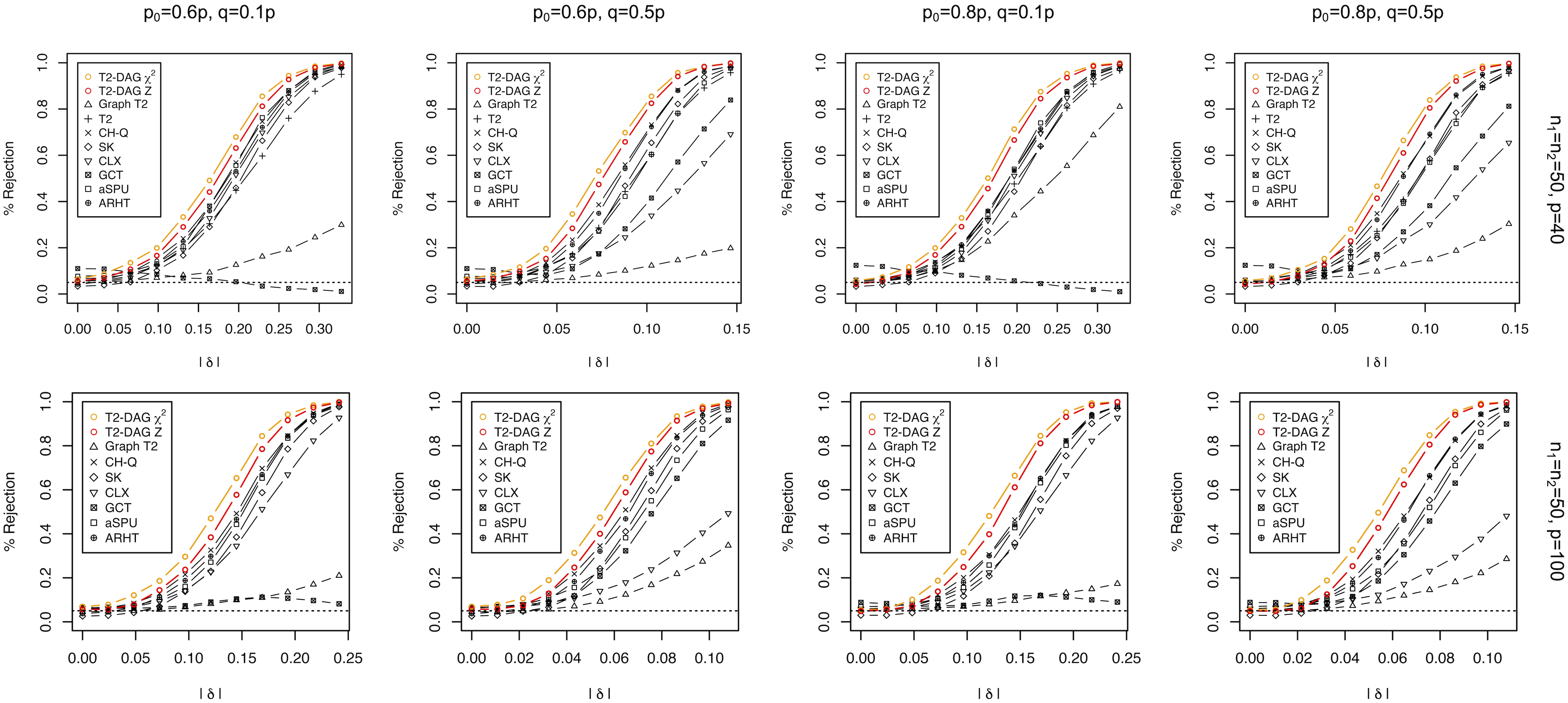
Figure 2: Empirical type I error rates ($\delta=0$) and powers ($|\delta|>0)$ under $n_{1}=n_{2}=50$ and $p=40$ (top row) or 100 (bottom row), with the number of children nodes in the DAG set to $p_{0}=0.6p$ (columns 1 and 2) or $p_{0}=0.8p$ (columns 3 and 4), and the number of non-zero signals set to $q=0.1p$ (columns 1 and 3) or $0.5p$ (columns 2 and 4).

Among the existing tests, CH-Q gives the best overall performance with a power higher than or equal to that of the Hotelling’s $T^{2}$ test (when $n_{1}+n_{2}>p$). The ARHT test shows a power that is similar to or slightly lower than that of the CH-Q test but higher than that of all other existing tests under all simulated scenarios, except for one scenario where aSPU has a slightly higher power (see Fig. 2, row 1, column 3). The Graph T2 test shows relatively low power in all scenarios. This is possibly because the simulated signal distribution is less coherent with the top eigenvectors of the graph Laplacian matrix. The power of the supremum-based CLX test is competitive to that of CH-Q and SK in sparse-signal scenarios (Fig. 2, columns 1 and 3), but is outperformed by most of the other tests under dense signals (Fig. 2, columns 2 and 4). The GCT test has an extremely low power in the sparse-signal scenarios (Fig. 2, columns 1 and 3), where the power is below 0.15 and even decreases as signal strength ($|\delta|$) increases. The proposed T2-DAG tests have substantially higher powers compared to the other tests in all simulated scenarios, except when signals are weak such that all tests have powers below 0.15. Compared to the T2-DAG $Z$ test that has a type I error rate strictly controlled at around $\alpha=0.05$, T2-DAG $\chi^{2}$ has a slightly higher but still well-controlled type I error rate and a higher power under all simulated scenarios. Furthermore, compared to the scenarios of $p_{0}=0.6p$ where there are condensed gene interactions towards a relatively small number of genes (Fig. 2, columns 1-2), in the scenarios of $p_{0}=0.8p$ where there are scattered gene interactions towards a larger number of genes (Fig. 2, columns 3-4), the two T2-DAG tests show more obvious advantages compared to the existing tests with strict type I error control and more improvement in power.

3.3 Results given partially incorrect edge information

We next discuss a more realistic scenario where the auxiliary edge information comes with errors, such as having missing and/or redundant edges. Recall that $N_{e}=\sum_{i=1}^{p}|S_{j}|$ denotes the total number of edges in the gene pathway. Besides the true adjacency matrix $A$, we consider two types of mis-specified auxiliary DAGs with the following adjacency matrices: (1) $A_{1}$ with a random set of $0.4N_{e}$ edges missing, and (2) $A_{2}$ with a random set of $0.4N_{e}$ redundant edges that do not exist in $A$. We implemented the proposed T2-DAG test based on $A$, $A_{1}$ or $A_{2}$, and implemented Graph T2 only based on the signed graph corresponding to the true adjacency matrix $A$.

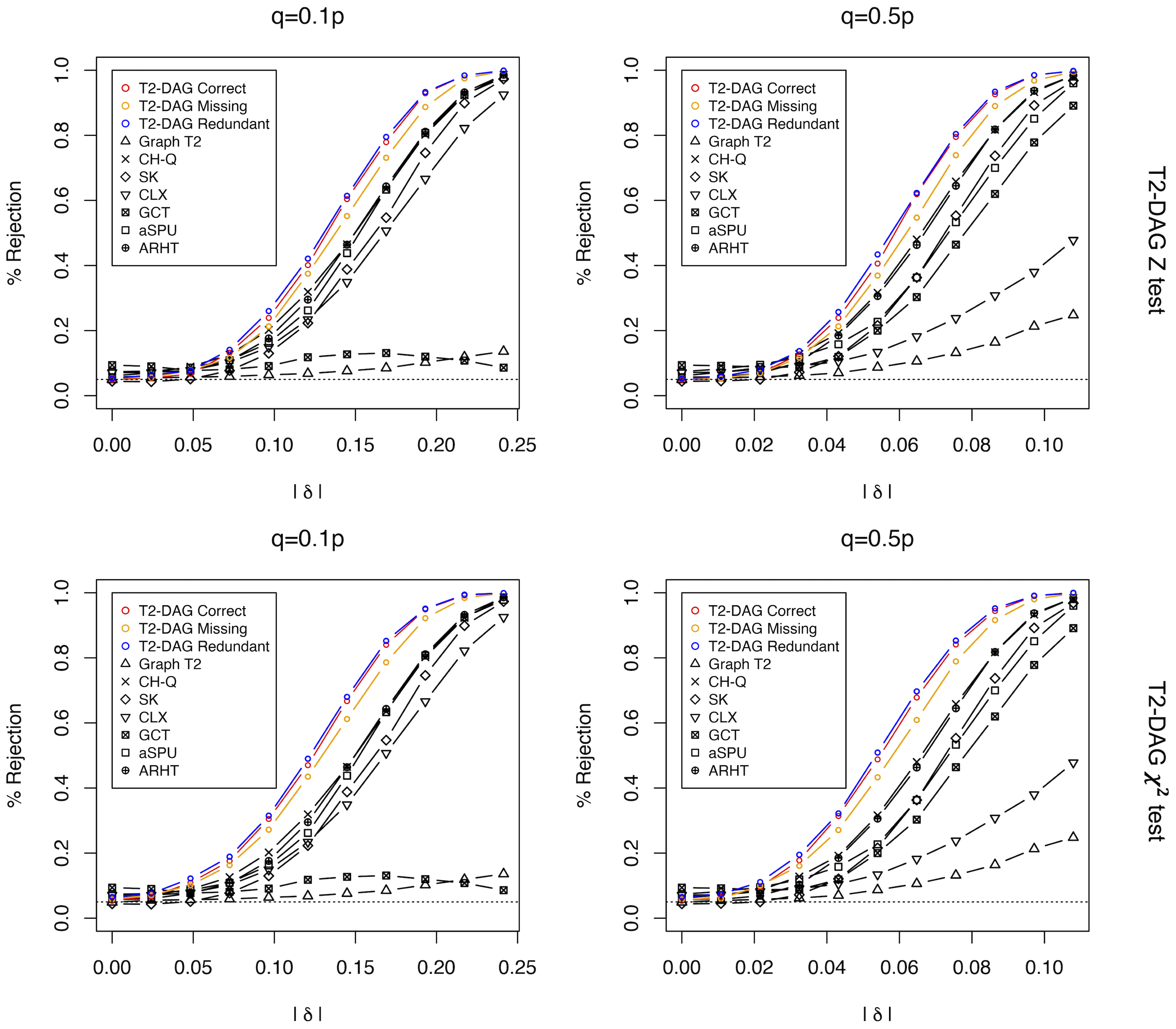
Figure 3: Empirical type I error rates ($\delta=0$) and powers ($|\delta|>0)$ of T2-DAG $Z$ (top panel) and T2-DAG $\chi^{2}$ (bottom panel) under $n_{1}=n_{2}=50$ and $p=100$, with the number of children nodes set to $p_{0}=0.8p$ and the number of non-zero signals set to $q=0.1p$ (column 1) or $0.5p$ (column 2). T2-DAG was applied based on $A$ (“T2-DAG Correct”), $A_{1}$ (“T2-DAG Missing”), or $A_{2}$ (“T2-DAG Redundant”). Graph T2 was applied based on the true adjacency matrix $A$.

Fig. 3 shows the empirical type I error rates and powers of all the tests given $n_{1}=n_{2}=50$ and $p=100$. Additional simulation results for $n_{1}=n_{2}=50$ and $p=50$, $n_{1}=n_{2}=100$ and $p=100$ or 300 are summarized in Figs. S4-S6. Although having incorporated the correct edge information as well as the signs of interactions, Graph T2 still has a much lower power compared to T2-DAG. Among the other existing tests that do not incorporate external graphical information, the ARHT test shows the highest power which is almost the same as that of CH-Q under relatively weak signals ($|\delta|$) and slightly higher than that of CH-Q under stronger signals. Similar to what we observed in Section 3.2, T2-DAG $\chi^{2}$ has well-controlled but slightly higher type I error rates and substantially higher power than T2-DAG $Z$. Using either of the two test statistics, the T2-DAG test based on pathway information with redundant edges (T2-DAG redundant) has slightly higher inflation in type I error rates, and the one based on partially missing edge information (T2-DAG Missing) has slightly compromised powers. Nonetheless, the overall performance of T2-DAG is similar across the three scenarios. This indicates the robustness of the proposed T2-DAG test with respect to potential errors in the auxiliary pathway information.

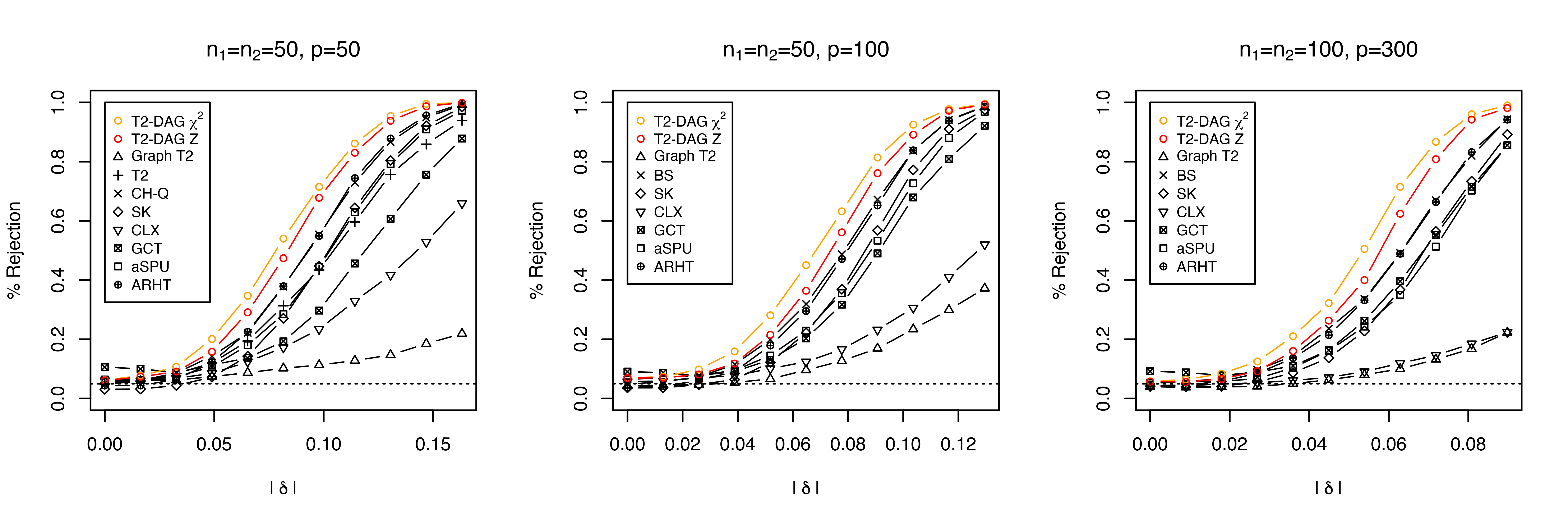
Figure 4: Empirical type I error rates ($\delta=0$) and powers ($|\delta|>0)$ of the various test assuming two continuous confounders, with the number of children nodes in the DAG set to $p_{0}=0.8p$, and the number of non-zero signals set to $q=0.5p$. Please note that the Hotelling’s $T^{2}$ test (T2) is not presented in columns 2 and 3 because it is not applicable when $n_{1}+n_{2}\leq p$.

3.4 Results in the presence of unadjusted confounding effects

So far, we have considered independent error terms $\epsilon_{j}\mathrel{\mathop{\mathchar 58\relax}}j=1,\ldots,p$, with a diagonal covariance matrix $R$. However, when there exist latent confounders affecting gene interactions, the error terms may be correlated, leading to a non-diagonal $R$. To evaluate the sensitivity of T2-DAG with respect to the mis-specification of $R$, we conducted additional simulations with two continuous confounders. Specifically, we generated two groups of gene expression data according to ${\bf x}_{i}^{(l)}=(I-Q^{\intercal})^{-1}(C^{\intercal}\bm{w}_{i}+{{\mbox{\boldmath${\epsilon}$}}}_{i})+\bm{\mu}_{l}$, $l=1,2$, $i=1,\ldots,n_{l}$. Here, $\bm{\mu}_{1}$, $\bm{\mu}_{2}$, $Q$ and ${{\mbox{\boldmath${\epsilon}$}}}_{i}$ were generated following the same procedure described in Section 3.1. The confounding variables $\bm{w}_{i}=(w_{i,1},w_{i,2})^{\intercal}$, $i=1,\ldots,n_{1}+n_{2}$, were generated independently from $\mathcal{N}(0,\Sigma_{w})$ with $\Sigma_{w}=\text{diag}((0.2)^{2}/\|Q\|_{\max})$. Twenty percent of the entries in each row of $C$ were generated independently from $\mathcal{N}(0,\sqrt{0.2})$, and the remaining entries were set to 0. As such, a random set of $0.2p$ genes were conditionally associated with each confounder. For T2-DAG test, we assumed that the confounders ${\mbox{\boldmath${w}$}}_{i}$ were latent, and T2-DAG was still implemented based on model (2).

We observe from Fig. 4 that all tests have well-controlled type I error rates expect for GCT, which shows high inflation in type I error rates. When the signals are not too weak (i.e., $|\delta|>0.05$), T2-DAG is more powerful than all other tests implemented. Additional simulation results based on $n_{1}=n_{2}=50$, $p=50$ and $n_{1}=n_{2}=100$, $p=100$ have similar patterns and are summarized in Fig. S7. These results show that T2-DAG can still outperform the existing tests even with unadjusted confounders.

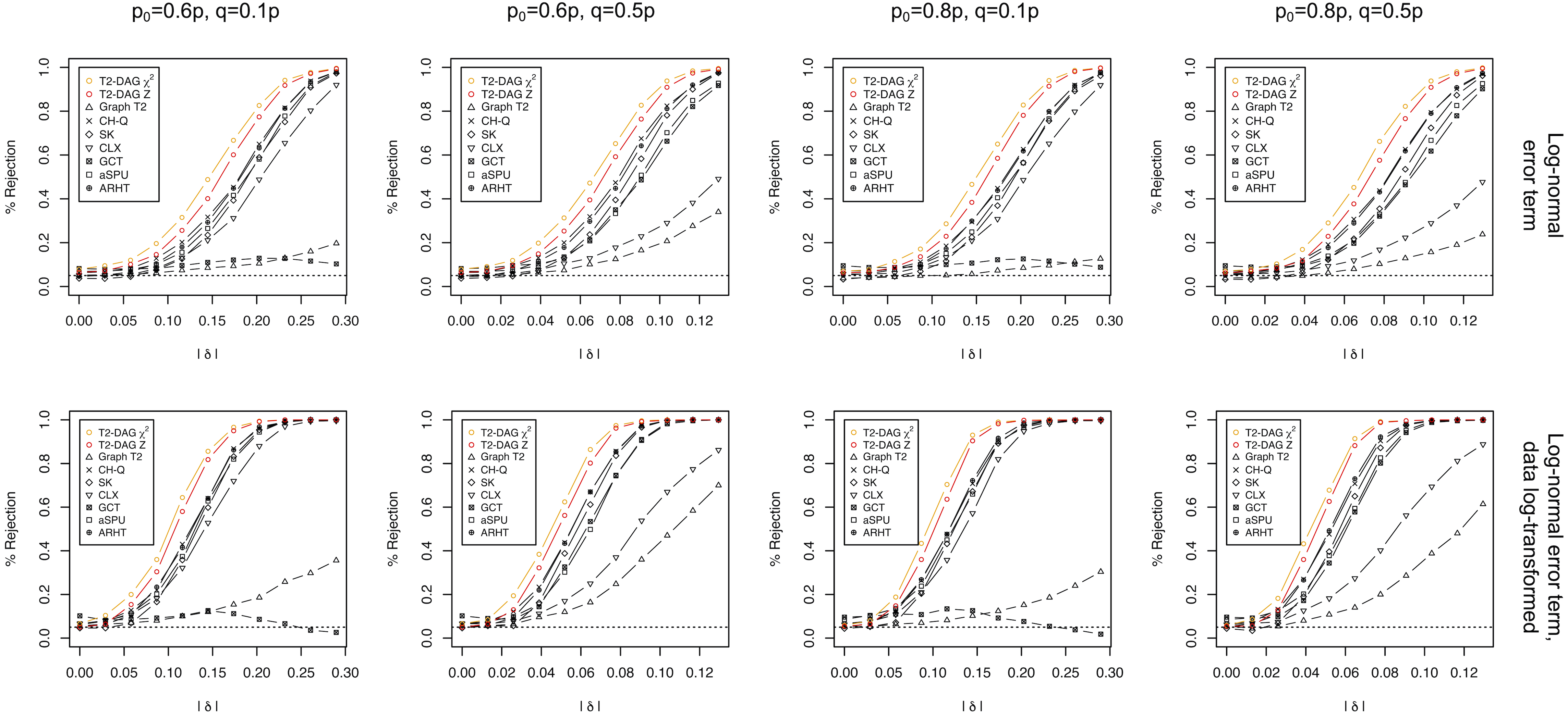
Figure 5: Empirical type I error rates ($\delta=0$) and powers ($|\delta|>0)$ of the various tests under ${n_{1}=n_{2}=50}$ and ${p=100}$ with error terms generated from log-normal distributions based on the raw data (row 1) or log-transformed data (row 2). The number of children nodes in the DAG is set to $p_{0}=0.6p$ (columns 1 and 2) or $p_{0}=0.8p$ (columns 3 and 4), and the number of non-zero signals is set to $q=0.1p$ (columns 1 and 3) or $0.5p$ (columns 2 and 4). Additional results under different settings of $n_{1}$, $n_{2}$, $p$ and results assuming error terms of gamma or uniform distributions are summarized in Figs. S8 - S18.

3.5 Results given non-Gaussian error terms

The theory of T2-DAG requires the assumption of Gaussian error terms, which can be violated in reality. We therefore conducted an additional sensitivity analysis on T2-DAG where we considered three alternative distributions: log-normal distribution, gamma distribution, and uniform distribution. Detailed simulation settings are summarized in Section 2.4 of the supplementary material. We can observe from the first row of Fig. 5 and Figs. S8 - S18 that T2-DAG tests perform similarly as in Section 3.2 with well-controlled type I error rates and higher powers than the existing tests, showing the robustness of T2-DAG to these distributions of the error terms. We further conducted a log transformation on the data under the scenarios of log-normal and gamma error terms where the simulated gene expression data were right skewed. Interestingly, this additional data transformation step lead to a substantial gain in power for all tests including T2-DAG in all scenarios, except for GCT in a few scenarios where it had powers lower than 0.15 under all signal strengths (Figs. 5 and S8 - S14, bottom row). Furthermore, while there is no obvious change in the type I error rates of the existing tests, T2-DAG consistently has a similar or more strict type I error control after the log transformation. These findings suggest that for right skewed gene expression data which is commonly seen in genetics studies we can conduct a log transformation to improve the performance of T2-DAG.

4 A real data example

In lung cancer diagnosis and prognosis, extensive research has been conducted utilizing gene expression profiling to identify lung cancer-related gene pathways for therapeutic research (Weiss and Kingsley, 2008; Shao et al., 2010; Cai and Jiang, 2014; Dancik and Theodorescu, 2014; Chang et al., 2015; Long et al., 2019; Venugopal et al., 2019; Kong et al., 2020). In this application, we aim to identify differentially expressed gene pathways between different stages of lung cancer, the findings of which could provide insights into the underlying genetic mechanisms of lung cancer progression.

We applied T2-DAG $Z$ and T2-DAG $\chi^{2}$, as well as the existing tests considered in the simulation studies, to a gene expression dataset for lung cancer patients in The Cancer Genome Atlas (TCGA) Program (Network et al., 2014). The dataset was obtained from the Lung Cancer Explorer (LCE) (Quantitative Biomeical Research Center, 2019) with standard quality control, where the expression values of zero were set to the overall minimum value and all data were then $\log_{2}$-transformed so that the gene expression data are approximately normal for all lung cancer stages (Cai et al., 2014, 2019). Expression levels of 20429 genes were measured for lung cancer tissue samples collected from 513 patients, among whom $N_{1}=278$, $N_{2}=124$, $N_{3}=84$ and $N_{4}=27$ were diagnosed with stage I, II, III and IV lung cancer, respectively. Additionally, $N_{0}=59$ normal tissue samples were collected from 59 of the 513 patients. When comparing cancer tissues with normal tissues, we excluded the tumor samples of these 59 patients to avoid dependent samples.

We considered $H=206$ common human pathways related to signaling, metabolic and human diseases from the KEGG database (Kanehisa and Goto, 2000; Kanehisa et al., 2019). Pathway information on previously identified gene interactions is categorized into activation/expression or inhibition/repression of one gene by another (Kanehisa and Goto, 2000; Kanehisa et al., 2019); see Fig. 1 for an illustrative example. Detailed characteristics of the pathways are summarized in Table S1. Among the 206 pathways, 34 have circles (including self loops) in the corresponding graphs, among which 18 has 1 circle only, 8 have 2 circles, 4 have 3 circles, and 4 have more than 3 circles each. We removed these circles when implementing the proposed T2-DAG test but used the complete graph information when implementing the Graph T2 test. Other than this, all the tests were implemented in the same way as in Section 3. We further applied Bonferroni correction (Bonferroni, 1936) with a significance level $\alpha=\alpha_{0}/H$ for each test to control the family-wise error rate (FWER) at $\alpha_{0}=0.05$.

Table 1: Results of the hypothesis tests on 206 KEGG pathways for differential gene expression between stage I and stage III lung cancer (top panel, $N_{1}=278$, $N_{3}=84$) and between stages II and stage III lung cancer (bottom panel, $N_{2}=124$, $N_{3}=84$). In each panel, the numbers on the diagonal line are the numbers of significant pathways identified by the corresponding methods; the numbers in the $(i,j)$-th cell in the upper and lower triangle are the number of significant pathways detected by both method $i$ and method $j$ and the estimated correlation of $-{\log}_{10}(p)$ between the two methods, respectively. “T2” denotes the Hotelling’s $T^{2}$ test.

Stage I versus Stage III
	T2-DAG $\chi^{2}$	T2-DAG $Z$	Graph T2	T2	CH-Q	SK	CLX	GCT	aSPU	ARHT
T2-DAG $\chi^{2}$	127	127	10	6	90	59	1	79	84	37
T2-DAG $Z$	0.98	144	10	8	93	59	1	82	88	37
Graph T2	0.43	0.45	10	2	8	8	0	7	8	5
T2	0.23	0.23	0.54	8	5	4	0	3	7	6
CH-Q	0.57	0.59	0.27	0.19	96	55	1	64	81	36
SK	0.75	0.77	0.48	0.43	0.58	59	0	41	50	28
CLX	0.54	0.56	0.42	0.34	0.54	0.60	1	0	1	1
GCT	0.81	0.76	0.40	0.17	0.36	0.63	0.29	82	59	27
aSPU	0.51	0.55	0.38	0.27	0.68	0.56	0.58	0.32	95	35
ARHT	0.56	0.56	0.26	0.20	0.70	0.48	0.46	0.37	0.57	37
Stage II versus Stage III
	T2-DAG $\chi^{2}$	T2-DAG $Z$	Graph T2	T2	CH-Q	SK	CLX	GCT	aSPU	ARHT
T2-DAG $\chi^{2}$	0	0	0	0	0	0	0	0	0	0
T2-DAG $Z$	-0.21	0	0	0	0	0	0	0	0	0
Graph T2	0.42	-0.24	0	0	0	0	0	0	0	0
T2	0.34	-0.30	0.54	0	0	0	0	0	0	0
CH-Q	0.48	-0.27	0.23	0.21	0	0	0	0	0	0
SK	-0.27	0.84	-0.31	-0.35	-0.34	0	0	0	0	0
CLX	0.63	-0.24	0.49	0.42	0.38	-0.26	0	0	0	0
GCT	-0.20	0.49	-0.21	-0.21	-0.18	0.58	-0.22	21	0	0
aSPU	0.43	-0.17	0.20	0.17	0.68	-0.20	0.44	-0.15	1	0
ARHT	0.33	-0.31	0.53	0.94	0.41	-0.35	0.44	-0.20	0.30	0

All tests except aSPU conclude that all 206 gene pathways are differentially expressed between normal tissues and tissues of each cancer stage (Tables S7 - S10). Table 1 summarizes the number of differentially expressed gene pathways detected by each test between stage I and stage III lung cancer and between stage II and stage III lung cancer. For the comparison between stage I and stage III lung cancer, the sample sizes ($N_{1}=278$, $N_{2}=124$) are large relative to the corresponding $p$, $p_{0}$ and $d$ for all pathways. The Hotelling’s $T^{2}$ test and Graph T2 test identify 8 and 10 significant pathways, respectively, while CH-Q, aSPU, GCT, SK and ARHT identify much more pathways (i.e., 96, 95, 82, 59 and 37, respectively). On the other hand, the CLX test, which is powerful for detecting sparse signals, only identifies 1 significant pathway. This may indicate that the signals of differential gene expression in real pathways tend to be dense, i.e., scatter among many correlated genes. The existing tests in total identify 129 unique pathways, while the T2-DAG $\chi^{2}$ test and $Z$ test identify 127 and 144 significant pathways, respectively, which cover 115 and 122, respectively, of the 129 pathways identified by the existing tests. Furthermore, the $-{\log}_{10}$-transformed p-values ($-{\log}_{10}p$) of the T2-DAG tests are positively correlated with those of all the other tests; in particular, results of T2-DAG tests are in line with those of CH-Q, SK, CLX, GCT, aSPU and ARHT, with correlations higher than 0.5. The two T2-DAG tests yield highly correlated results (the correlation of $-{\log}_{10}p$ equals 0.98). T2-DAG $Z$ detects a slightly larger number of significant pathways than T2-DAG $\chi^{2}$, and for the pathways detected by both tests, T2-DAG $Z$ tends to give smaller p-values than T2-DAG $\chi^{2}$. This is different from what was observed from simulations where T2-DAG $Z$ tends to have lower rejection rates than T2-DAG $\chi^{2}$, which could be due to the difference in data structures between the simulated data and real data. This inconsistency in relative performance is observed not only for the two T2-DAG tests, but also for other tests such as CH-Q and ARHT, which perform similarly on the simulated data but yield quite different results on the lung cancer data where they detect 96 and 37 differentially expressed pathways, respectively, between stage I and stage III lung cancer.

For the comparison between stage II and stage III lung cancer, all tests except GCT and aSPU detect no differentially expressed gene pathway. This may be due to the limited sample sizes ($N_{3}=124$, $N_{4}=84$) and/or relatively small differences between stage II and stage III lung cancer. On the other hand, aSPU identifies 1 significant pathway, while GCT identifies 21 significant pathways that do not include the one identified by aSPU. These 21 pathways are possibly false positives because of two reasons. First, none of the pathways is detected by any other test. Second, in our simulation studies, GCT could have substantially inflated type I error rates under small $p$ settings (Fig. 2, Fig. 4, Fig. S1 and Fig. S7).

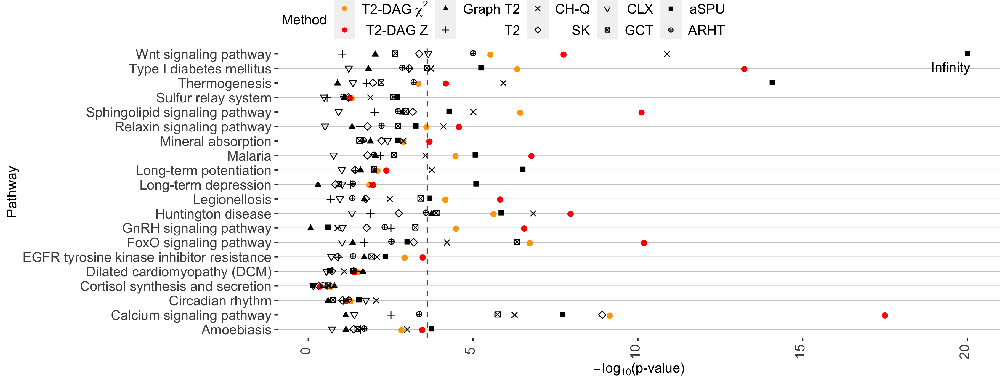
Figure 6: $-{\log}_{10}(p)$ of the various tests for differential expression between stage I and stage III lung cancer on 20 randomly selected human pathways.

To take a closer look at these results, we randomly selected 20 of the 206 pathways and report the corresponding $-{\log}_{10}(p)$s (Fig. 6: stage I versus stage III; Fig. S18: stage II versus stage III). Overall, the p-values for comparison between stage I and stage III lung cancer show consistency across different tests. Specifically, for pathways on which all tests yield insignificant results with large p-values, the T2-DAG tests give similar and sometimes even larger p-values compared to the other tests; see the Sulfur relay system pathway and the Circadian rhythm pathway in Fig. 6. For pathways on which T2-DAG yields highly significant results with the smallest p-values, many of the other tests also yield significant results; see the Calcium signaling pathway and the Type I diabetes mellitus in Fig. 6. On the contrary, for the pathways identified by GCT to be significantly differentially expressed between stage II and stage III cancer, all the other tests yield insignificant results with large $p$-values (Fig. 7).

We also compared other pairs of cancer stages and summarized the results in Section 3 of the supplementary material. Results for the comparison of stage I versus II, stage I versus IV, and stage II versus IV cancer have similar patterns as the comparison between stage I and III cancer. Similar to the comparison between stage II and III cancer, when comparing stage III to stage IV cancer, none of the tests identifies any significant pathway except for GCT which identifies 5 significant pathways. Detailed results for all the tests are summarized in Tables S1 - S10.

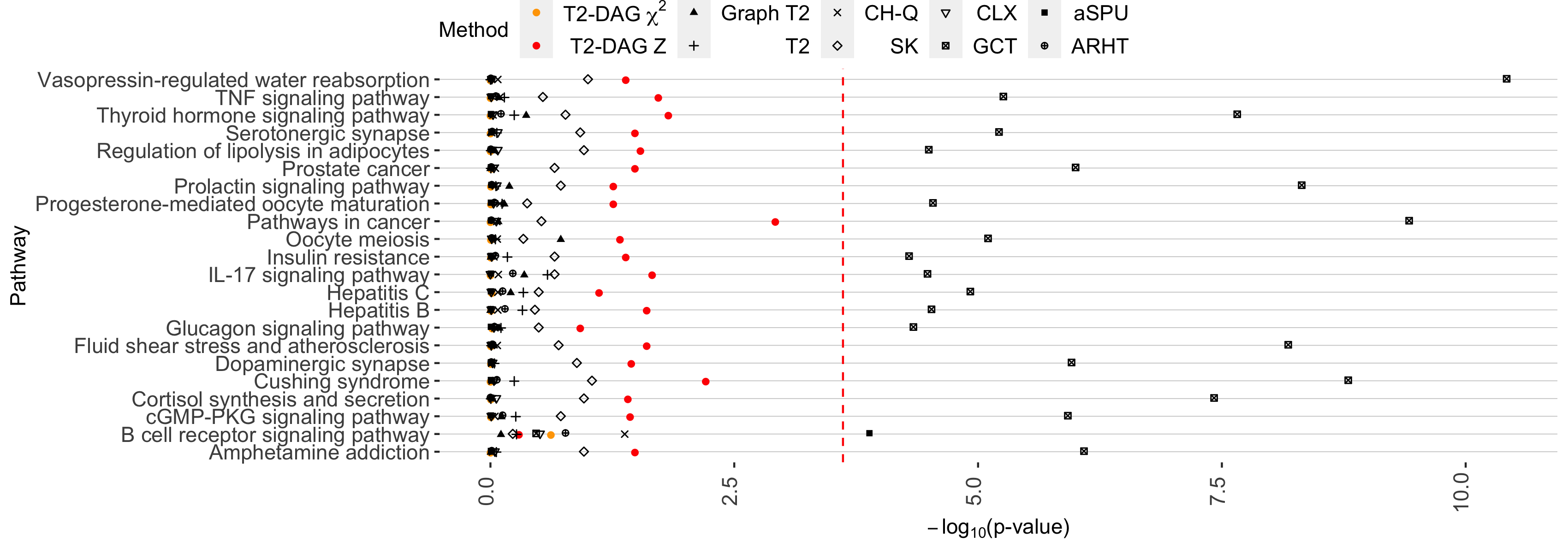
Figure 7: The $-{\log}_{10}(p)$ of the comparison between stage II and stage III lung cancer ($N_{2}=124$, $N_{3}=84$) for the pathways identified by any test to be significantly differentially expressed between the two cancer stages.

5 Discussion

The proposed T2-DAG $Z$ test and the alternative T2-DAG $\chi^{2}$ test have illustrated their advantages over the existing tests through our simulation studies and application to a lung cancer dataset. When establishing asymptotic properties, the T2-DAG $Z$ test is favored over the alternative T2-DAG $\chi^{2}$ test since it requires less stringent conditions and thus is presented as our main result. Although facing theoretical limitations, the alternative T2-DAG $\chi^{2}$ test has excellent finite-sample performance where it has slightly higher but still well-controlled type I error rates and higher powers than T2-DAG $Z$, as shown by simulations. In the lung cancer application, however, T2-DAG $\chi^{2}$ appears to be slightly more conservative than T2-DAG $Z$ but still identifies a much larger number of differentially expressed pathways than the existing tests for stage I versus stage II, III, or IV cancer. In applications, the choice between T2-DAG $Z$ and T2-DAG $\chi^{2}$ can be made based on the theoretical properties and simulated finite-sample results under the specific data scenarios of sample size ($n_{1}$ and $n_{2}$), dimension ($p$), and sparsity of gene interactions ($p_{0}$ and $d$) inferred from the auxiliary pathway information.

The proposed T2-DAG test was motivated by gene pathway analyses, but it is generally applicable to problems in many other areas where similar auxiliary graph information is available. For example, in human microbiome studies for identifying host-microbe associations, the auxiliary graph information is provided by the phylogenetic tree that characterizes the evolutionary relationships among the microbes.

We have illustrated the robustness of T2-DAG with respective to model mis-specifications due to missing/inaccurate edge information or unadjusted confounding effects. While our simulation results are encouraging in these scenarios, the current estimation procedure may no longer be optimal. Thus, we consider the following two extensions of T2-DAG as our future work. First, while T2-DAG requires that the auxiliary pathway information can be represented by a DAG, it is feasible to extend it to non-DAG pathways with more complex gene interactions. For example, the recently proposed linear SEM for cyclic mixed graphs (Améndola et al., 2020) shows a possible way to account for feedback loops and undirected edges in the gene pathway. Second, the proposed test assumes a diagonal covariance matrix $R$ for the error term ${\epsilon}$ in (2). As discussed in Section 3.4, this assumption may fail due to latent confounders. In this case, we may consider a non-diagonal but sparse $R$, i.e., only a small number of off-diagonal entries of $R$ are non-zero, and estimate $R$ via graphical lasso (Friedman et al., 2008) or other penalized estimation approaches for high-dimensional precision matrix (Zhang and Zou, 2014; Kuismin et al., 2017; Fan et al., 2019). Furthermore, when measurements are available for some potential confounders, we can directly incorporate them into the SEM as covariates. We have in fact observed promising performance of this strategy through additional simulation studies, but the theoretical properties of the strategy require further investigation.

While the current T2-DAG test only incorporates information on the presence/absence of gene interactions, it is possible to further incorporate the signs of the interactions, such as activation ($+$) or inhibition ($-$) of one gene by another. One possible strategy is to conduct modeling in a Bayesian framework, where the signs of gene interactions can be accounted for by inducing truncated normal priors on the corresponding parameters in the coefficient matrix $Q$. The asymptotic properties of the test, however, need to be re-investigated.

Finally, we note that the key component of the proposed T2-DAG test is the novel DAG-informed estimator for the precision matrix (see Equations (3) and (4)), which could provide substantially improved power through incorporating external pathway information that describes gene interactions. Besides being incorporated into our T2-DAG test, this novel estimator has plenty of other potential usage. For example, as illustrated in Section 4, T2-DAG, with a Hotelling’s $T^{2}$-type test statistic, is powerful against “dense” alternatives which are usually true for differentially expressed gene pathways. In applications where the signals are sparse, one may instead consider combining the proposed DAG-informed estimator with tests that are powerful against “sparse” alternatives, such as the CLX test (Cai et al., 2014), to further boost power. Another example is that the proposed DAG-informed estimator can be used for high-dimensional linear discriminant analysis (LDA) (Bouveyron et al., 2007) to improve the classification accuracy. Specifically, consider the Gaussian case where one wants to classify a random vector $\bf x$ drawn with equal probability from one of the two Gaussian distributions, $\mathcal{N}({\mbox{\boldmath${\mu}$}}_{1},\Sigma)$ (class 1) and $\mathcal{N}({\mbox{\boldmath${\mu}$}}_{2},\Sigma)$ (class 2). When ${\mbox{\boldmath${\mu}$}}_{1},{\mbox{\boldmath${\mu}$}}_{2}$ and $\Sigma$ are known, Fisher’s LDA rule, given by

$$C(\bm{x})=\Bigg{\{}\begin{array}[]{ll}1,&~{}~{}~{}\bm{\delta}^{\top}\Omega\left(\bm{x}-\frac{\bm{\mu}_{1}+\bm{\mu}_{2}}{2}\right)<0\\ 2,&~{}~{}~{}\bm{\delta}^{\top}\Omega\left(\bm{x}-\frac{\bm{\mu}_{1}+\bm{\mu}_{2}}{2}\right)\geq 0,\end{array}$$

where ${\mbox{\boldmath${\delta}$}}={\mbox{\boldmath${\mu}$}}_{2}-{\mbox{\boldmath${\mu}$}}_{1}$, and $\Omega=\Sigma^{-1}$ denotes the precision matrix, is known to be optimal. In practice, one needs to estimate ${\mbox{\boldmath${\mu}$}}_{1},{\mbox{\boldmath${\mu}$}}_{2}$, and $\Omega$. The proposed DAG-informed estimator of $\Omega$ can thus be applied here to facilitate the classification.

Conflicts of Interest

The authors declare no conflict of interest.

Data Availability

The data underlying this article are available at https://github.com/Jin93/T2DAG.

Supplementary Material

Supplementary material available at Bioinformatics online includes technical results and proofs, detailed information on the pathways and gene expression data used in the data analysis, detailed simulation settings in the scenario of non-Gaussian error terms, as well as additional results on the simulated and real datasets.

Software

The R (R Development Core Team, 2021) package T2DAG which implements the proposed T2-DAG test is available on Github at https://github.com/Jin93/T2DAG.

References

- Améndola et al. (2020) C. Améndola, P. Dettling, M. Drton, F. Onori, and J. Wu. Structure learning for cyclic linear causal models. In Conference on Uncertainty in Artificial Intelligence, pages 999–1008. PMLR, 2020.
- Ashburner et al. (2000) M. Ashburner, C. A. Ball, J. A. Blake, D. Botstein, H. Butler, J. M. Cherry, A. P. Davis, K. Dolinski, S. S. Dwight, J. T. Eppig, et al. Gene ontology: tool for the unification of biology. Nature genetics, 25(1):25–29, 2000.
- Bai and Saranadasa (1996) Z. Bai and H. Saranadasa. Effect of high dimension: by an example of a two sample problem. Statistica Sinica, pages 311–329, 1996.
- Bonferroni (1936) C. Bonferroni. Teoria statistica delle classi e calcolo delle probabilita. Pubblicazioni del R Istituto Superiore di Scienze Economiche e Commericiali di Firenze, 8:3–62, 1936.
- Bouveyron et al. (2007) C. Bouveyron, S. Girard, and C. Schmid. High-dimensional discriminant analysis. Communications in Statistics—Theory and Methods, 36(14):2607–2623, 2007.
- Cai and Jiang (2014) B. Cai and X. Jiang. Revealing biological pathways implicated in lung cancer from tcga gene expression data using gene set enrichment analysis. Cancer Informatics, 13:CIN–S13882, 2014.
- Cai et al. (2019) L. Cai, S. Lin, L. Girard, Y. Zhou, L. Yang, B. Ci, Q. Zhou, D. Luo, B. Yao, H. Tang, et al. Lce: an open web portal to explore gene expression and clinical associations in lung cancer. Oncogene, 38(14):2551–2564, 2019.
- Cai et al. (2014) T. T. Cai, W. Liu, and Y. Xia. Two-sample test of high dimensional means under dependence. Journal of the Royal Statistical Society: Series B (Statistical Methodology), 76(2):349–372, 2014.
- Chang et al. (2015) J. T.-H. Chang, Y. M. Lee, and R. S. Huang. The impact of the cancer genome atlas on lung cancer. Translational Research, 166(6):568–585, 2015.
- Chen et al. (2011) L. S. Chen, D. Paul, R. L. Prentice, and P. Wang. A regularized hotelling’s t 2 test for pathway analysis in proteomic studies. Journal of the American Statistical Association, 106(496):1345–1360, 2011.
- Chen and Qin (2010) S. X. Chen and Y.-L. Qin. A two-sample test for high-dimensional data with applications to gene-set testing. The Annals of Statistics, 38(2):808–835, 2010.
- Chun et al. (2015) H. Chun, X. Zhang, and H. Zhao. Gene regulation network inference with joint sparse gaussian graphical models. Journal of Computational and Graphical Statistics, 24(4):954–974, 2015.
- Consortium (2019) G. O. Consortium. The gene ontology resource: 20 years and still going strong. Nucleic acids research, 47(D1):D330–D338, 2019.
- Dancik and Theodorescu (2014) G. M. Dancik and D. Theodorescu. Robust prognostic gene expression signatures in bladder cancer and lung adenocarcinoma depend on cell cycle related genes. PloS one, 9(1):e85249, 2014.
- Fan et al. (2019) R. Fan, B. Jang, Y. Sun, and S. Zhou. Precision matrix estimation with noisy and missing data. In The 22nd International Conference on Artificial Intelligence and Statistics, pages 2810–2819. PMLR, 2019.
- Friedman et al. (2008) J. Friedman, T. Hastie, and R. Tibshirani. Sparse inverse covariance estimation with the graphical lasso. Biostatistics, 9(3):432–441, 2008.
- Gregory et al. (2015) K. B. Gregory, R. J. Carroll, V. Baladandayuthapani, and S. N. Lahiri. A two-sample test for equality of means in high dimension. Journal of the American Statistical Association, 110(510):837–849, 2015.
- Hotelling (1931) H. Hotelling. The generalization of student’s ratio. The Annals of Mathematical Statistics, 2(3):360–378, 1931.
- Huang et al. (2006) J. Z. Huang, N. Liu, M. Pourahmadi, and L. Liu. Covariance matrix selection and estimation via penalised normal likelihood. Biometrika, 93(1):85–98, 2006.
- Jacob et al. (2012) L. Jacob, P. Neuvial, and S. Dudoit. More power via graph-structured tests for differential expression of gene networks. The Annals of Applied Statistics, 6(2):561–600, 2012.
- Kanehisa and Goto (2000) M. Kanehisa and S. Goto. Kegg: kyoto encyclopedia of genes and genomes. Nucleic acids research, 28(1):27–30, 2000.
- Kanehisa et al. (2019) M. Kanehisa, Y. Sato, M. Furumichi, K. Morishima, and M. Tanabe. New approach for understanding genome variations in kegg. Nucleic acids research, 47(D1):D590–D595, 2019.
- Kong et al. (2020) C. Kong, Y.-X. Yao, Z.-T. Bing, B.-H. Guo, L. Huang, Z.-G. Huang, and Y.-C. Lai. Dynamical network analysis reveals key micrornas in progressive stages of lung cancer. PLOS Computational Biology, 16(5):e1007793, 2020.
- Krishnamoorthy and Menon (2013) A. Krishnamoorthy and D. Menon. Matrix inversion using cholesky decomposition. In 2013 signal processing: Algorithms, architectures, arrangements, and applications (SPA), pages 70–72. IEEE, 2013.
- Kuismin et al. (2017) M. Kuismin, J. Kemppainen, and M. Sillanpää. Precision matrix estimation with rope. Journal of Computational and Graphical Statistics, 26(3):682–694, 2017.
- Li et al. (2012) B. Li, H. Chun, and H. Zhao. Sparse estimation of conditional graphical models with application to gene networks. Journal of the American Statistical Association, 107(497):152–167, 2012.
- Li et al. (2020) H. Li, A. Aue, D. Paul, J. Peng, and P. Wang. An adaptable generalization of hotelling’s test in high dimension. The Annals of Statistics, 48(3):1815–1847, 2020.
- Loh and Bühlmann (2014) P.-L. Loh and P. Bühlmann. High-dimensional learning of linear causal networks via inverse covariance estimation. The Journal of Machine Learning Research, 15(1):3065–3105, 2014.
- Long et al. (2019) T. Long, Z. Liu, X. Zhou, S. Yu, H. Tian, and Y. Bao. Identification of differentially expressed genes and enriched pathways in lung cancer using bioinformatics analysis. Molecular medicine reports, 19(3):2029–2040, 2019.
- Lopes et al. (2011) M. Lopes, L. Jacob, and M. J. Wainwright. A more powerful two-sample test in high dimensions using random projection. In Advances in Neural Information Processing Systems, pages 1206–1214, 2011.
- Love et al. (2014) M. I. Love, W. Huber, and S. Anders. Moderated estimation of fold change and dispersion for rna-seq data with deseq2. Genome biology, 15(12):550, 2014.
- Network et al. (2014) C. G. A. R. Network et al. Comprehensive molecular profiling of lung adenocarcinoma. Nature, 511(7511):543–550, 2014.
- Nishimura (2001) D. Nishimura. Biocarta. Biotech Software & Internet Report, 2(3):117–120, 2001. doi: 10.1089/152791601750294344. URL https://doi.org/10.1089/152791601750294344.
- Peters and Bühlmann (2014) J. Peters and P. Bühlmann. Identifiability of gaussian structural equation models with equal error variances. Biometrika, 101(1):219–228, 2014.
- Quantitative Biomeical Research Center (2019) Quantitative Biomeical Research Center. Lung Cancer Explorer. http://lce.biohpc.swmed.edu/, 2019. Accessed: 2021-06-15.
- Robinson et al. (2010) M. D. Robinson, D. J. McCarthy, and G. K. Smyth. edger: a bioconductor package for differential expression analysis of digital gene expression data. Bioinformatics, 26(1):139–140, 2010.
- Shao et al. (2010) W. Shao, D. Wang, and J. He. The role of gene expression profiling in early-stage non-small cell lung cancer. Journal of thoracic disease, 2(2):89, 2010.
- Shojaie and Michailidis (2009) A. Shojaie and G. Michailidis. Analysis of gene sets based on the underlying regulatory network. Journal of Computational Biology, 16(3):407–426, 2009.
- Shojaie and Michailidis (2010) A. Shojaie and G. Michailidis. Network enrichment analysis in complex experiments. Statistical applications in genetics and molecular biology, 9(1), 2010.
- Srivastava and Du (2008) M. S. Srivastava and M. Du. A test for the mean vector with fewer observations than the dimension. Journal of Multivariate Analysis, 99(3):386–402, 2008.
- Srivastava and Kubokawa (2013) M. S. Srivastava and T. Kubokawa. Tests for multivariate analysis of variance in high dimension under non-normality. Journal of Multivariate Analysis, 115:204–216, 2013.
- Tibshirani (1996) R. Tibshirani. Regression shrinkage and selection via the lasso. Journal of the Royal Statistical Society: Series B (Methodological), 58(1):267–288, 1996.
- Venugopal et al. (2019) N. Venugopal, J. Yeh, S. K. Kodeboyina, T. J. Lee, S. Sharma, N. Patel, and A. Sharma. Differences in the early stage gene expression profiles of lung adenocarcinoma and lung squamous cell carcinoma. Oncology Letters, 18(6):6572–6582, 2019. doi: 10.3892/ol.2019.11013.
- Weiss and Kingsley (2008) G. J. Weiss and C. Kingsley. Pathway targets to explore in the treatment of non-small cell lung cancer. Journal of Thoracic Oncology, 3(11):1342–1352, 2008.
- Wille et al. (2004) A. Wille, P. Zimmermann, E. Vranová, A. Fürholz, O. Laule, S. Bleuler, L. Hennig, A. Prelić, P. von Rohr, L. Thiele, et al. Sparse graphical gaussian modeling of the isoprenoid gene network in arabidopsis thaliana. Genome biology, 5(11):R92, 2004.
- Wu and Pourahmadi (2003) W. B. Wu and M. Pourahmadi. Nonparametric estimation of large covariance matrices of longitudinal data. Biometrika, 90(4):831–844, 2003.
- Xu et al. (2016) G. Xu, L. Lin, P. Wei, and W. Pan. An adaptive two-sample test for high-dimensional means. Biometrika, 103(3):609–624, 2016.
- Zhang and Zou (2014) T. Zhang and H. Zou. Sparse precision matrix estimation via lasso penalized d-trace loss. Biometrika, 101(1):103–120, 2014.