Sparse Spectral-Galerkin Method on An Arbitrary Tetrahedron Using Generalized Koornwinder Polynomials

Abstract

In this paper, we propose a sparse spectral-Galerkin approximation scheme for solving the second-order partial differential equations on an arbitrary tetrahedron. Generalized Koornwinder polynomials are introduced on the reference tetrahedron as basis functions with their various recurrence relations and differentiation properties being explored. The method leads to well-conditioned and sparse linear systems whose entries can either be calculated directly by the orthogonality of the generalized Koornwinder polynomials for differential equations with constant coefficients or be evaluated efficiently via our recurrence algorithm for problems with variable coefficients. Clenshaw algorithms for the evaluation of any polynomial in an expansion of the generalized Koornwinder basis are also designed to boost the efficiency of the method. Finally, numerical experiments are carried out to illustrate the effectiveness of the proposed Koornwinder spectral method.

Keywords: generalized Koornwinder polynomials,  tetrahedron,  spectral-Galerkin method,  sparse,  well-conditioned

2020 Mathematics Subject Classification: 65N25,  65N35

1 Introduction

Spectral element methods with unstructured mesh have been widely used in the study of computational fluid dynamics, elastodynamics, resistivity modeling and many other fields due to their “spectral accuracy” [30, 17, 35, 22]. Their virtue of high accuracy also makes spectral (element) methods powerful tools for solving eigenvalue problems as they are able to provide more reliable eigen-solutions than the low order methods such as finite element methods and finite difference methods [34, 3]. Meanwhile, as simplices are one kind of the basic geometric elements, their use gives flexibility in the discretization of complex domains. In view of this, spectral methods on simplex elements, especially on tetrahedra in three dimensions, with sparse structures in discrete matrices, play a fundamental role in designing accurate and efficient numerical schemes in practical applications.

Based on the Galerkin framework, the accuracy and computational effectivity of the numerical scheme depend on the choice of basis functions. Hierarchical basis functions defined in the barycentric coordinate system on the tetrahedron have been proposed and developed in [25, 32, 8, 1], which possess good symmetry but lack useful orthogonality. Thus, it requires complicated numerical integration for obtaining linear systems in high order case. In the Cartesian coordinate system, although a fully tensorial spectral method using rational basis functions put forward in [20] has spectral accuracy in approximations and can be implemented effectively, the use of orthogonal basis polynomials is more natural. Koornwinder polynomials form a family of fully orthogonal polynomials with respect to a particular weight function on the simplex [18] and its simplest family, the $L^{2}$-orthogonal Koornwinder-Dubiner polynomials have been studied in [10]. Motivated by generalized Jacobi polynomials [13, 14, 29], some progress on numerical schemes and theoretical analysis have been made for generalized Koornwinder polynomials on triangles [19, 28, 24]. Indeed, generalized Koornwinder polynomials simplify the design of shape functions in triangular spectral element approximations with efficient numerical algorithms and well-conditioned sparse linear systems. However, few results are achieved for the extension of generalized Koornwinder polynomials to tetrahedra, although polynomial basis functions for tetrahedral elements have been proposed by Sherwin and Karniadakis based on classical Koornwinder polynomials in 1990’s [31, 17], and by Beuchler et al. based on integrated Jacobi polynomials in 2000’s [6, 4, 5].

In this paper, we first introduce the generalized Koornwinder polynomials on a reference tetrahedron and explore their various recurrence relations and differentiation properties. We then propose a sparse spectral-Galerkin method for second-order partial differential equations on an arbitrary tetrahedron by employing generalized Koornwinder polynomials to design modal basis functions in simple presentations. The sparsity that exists in various recurrence relations of generalized Koornwinder polynomials allows us to assemble the discrete matrices efficiently. Indeed, a generalized Koornwinder polynomial of certain order or its derivatives are equal to a finite combination of Koornwinder-Dubiner polynomials. For differential equations with constant coefficients, the integrals of two generalized Koornwinder polynomials or their derivatives, which are entries of the stiffness matrix and the mass matrix, can be exactly evaluated by the expansion coefficients and the $L^{2}$-orthogonality of Koornwinder-Dubiner polynomials. For the case of variable coefficients, the three-term recurrence relation for generalized Koornwinder polynomials yields a recursive assembling of the mass matrix that only requires $\mathcal{O}(M^{6})$ operations (for polynomials of total degree $\leq M$), instead of the complexity of $\mathcal{O}(M^{9})$ by directly using numerical quadrature. The three-term recurrence relation also admits an efficient implementation of the Clenshaw algorithm [9] to evaluate the generalized Koornwinder expansions in $\mathcal{O}(M^{3})$ operations. More importantly, a numerical study reveals that the sparse linear system resulted from our spectral-Galerkin method has a condition number asymptotically in $\mathcal{O}(M^{4})$, which is superior to $\mathcal{O}(M^{7})$ for those using classical Koornwinder polynomials and $\mathcal{O}(M^{10})$ for those using integrated Jacobi polynomials. Hence, our linear system is well-conditioned and can be efficiently solved.

The paper is organized as follows. In Section 2, we formulate definitions and basic properties of generalized Jacobi polynomials and generalized Koornwinder polynomials, including their various recurrence relations and differentiation properties. In Section 3, an efficient implementation of the Clenshaw algorithm for Koornwinder expansions based on the three-term recurrence relation of generalized Koornwinder polynomials has been studied. The sparse spectral-Galerkin method for second-order partial differential equations on an arbitrary tetrahedron using generalized Koornwinder polynomials together with its implementation is presented in Section 4. We report some illustrative numerical results to confirm the sparsity as well as exponential orders of convergence of the method in Section 5. Finally, a conclusion remark is given in Section 6.

2 Preliminaries

Let $\Omega\subset\mathbb{R}^{3}$ be a bounded domain and $w$ be a weight function. Denote by $(\cdot,\cdot)_{w,\Omega}$ and $\|\cdot\|_{w,\Omega}$ the inner product and the norm of $L^{2}_{w}(\Omega)$, respectively. $H_{w}^{s}(\Omega)$ and $H^{s}_{0,w}(\Omega)$ are the usual Sobolev spaces with respect to the weight function $w$. Denote by $\mathbb{Z}$, $\mathbb{N}$, $\mathbb{N}_{0}$ and $\mathbb{Z}^{-}$ the set of integers, positive integers, non-negative integers and negative integers, respectively. Further let $I_{m}\in\mathbb{R}^{m\times m}$ be the identity matrix and $\bm{e}_{n}$ be the unit column vector only with its $n$-th entry being 1.

For any $M\in\mathbb{N}_{0}$, let $\mathcal{P}_{M}(\Omega)$ be the space of polynomials of total degree no greater than $M$ in $\Omega$ and denote

$$d_{M}:=\dim\mathcal{P}_{M}(\Omega)=\binom{M+3}{M}.$$ (2.1)

$\Omega$ and $w$ (if $w\equiv 1$) could be dropped from the notation when no confusion would arise.

Let $\hat{\mathcal{T}}$ be the reference tetrahedron defined as

$$\hat{\mathcal{T}}:=\{\bm{\hat{x}}=(\hat{x}_{1},\hat{x}_{2},\hat{x}_{3})^{\mathsf{T}}:0\leq\hat{x}_{1},\hat{x}_{2},\hat{x}_{3},\hat{x}_{1}+\hat{x}_{2}+\hat{x}_{3}\leq 1\},$$

with vertices

$$\hat{P}_{0}=(0,0,0)^{\mathsf{T}},\quad\hat{P}_{1}=(1,0,0)^{\mathsf{T}},\quad\hat{P}_{2}=(0,1,0)^{\mathsf{T}},\quad\hat{P}_{3}=(0,0,1)^{\mathsf{T}}.$$

Moreover, let $\left(\bm{a}\cdot\bm{b}\right)$ and $\bm{a}\times\bm{b}$ denote the dot product and the cross product of any $\bm{a},\bm{b}\in\mathbb{R}^{3},$ respectively. Denote $(\bm{a},\bm{b},\bm{c})=\bm{a}\cdot(\bm{b}\times\bm{c})=\bm{b}\cdot(\bm{c}\times\bm{a})=\bm{c}\cdot(\bm{a}\times\bm{b})$ as the triple product of any $\bm{a},\bm{b},\bm{c}\in\mathbb{R}^{3}$. For any $\bm{\ell}=(\ell_{1},\ell_{2},\ell_{3})\in\mathbb{N}_{0}^{3}$ and $\bm{\alpha}=(\alpha_{0},\alpha_{1},\alpha_{2},\alpha_{3})\in\mathbb{R}^{4}$, we introduce the following multi-index notation

$$|\bm{\ell}|=\ell_{1}+\ell_{2}+\ell_{3}, |\bm{\alpha}|=\alpha_{0}+\alpha_{1}+\alpha_{2}+\alpha_{3},$$

$$\bm{\ell}^{i}=(\ell_{1},\cdots,\ell_{i}), |\bm{\ell}^{i}|=\ell_{1}+\cdots+\ell_{i} 1\leq i\leq 2,\,i\in\mathbb{N},$$

$$\bm{\alpha}^{j}=(\alpha_{0},\cdots,\alpha_{j}), |\bm{\alpha}^{j}|=\alpha_{0}+\cdots+\alpha_{j}, 0\leq j\leq 2,\,j\in\mathbb{N}_{0}.$$

2.1 Generalized Jacobi polynomials

Let $I=(-1,1)$. For any $k\in\mathbb{N}_{0}$, the classical Jacobi polynomial $J_{k}^{\alpha,\beta}(z)$ of degree $k$ with $\alpha,\beta>-1$ has the following representation in hypergeometric series,

$$J_{k}^{\alpha,\beta}(z)=\sum\limits_{j=0}^{k}\frac{(\alpha+j+1)_{k-j}(k+\alpha+\beta+1)_{j}}{j!(k-j)!}\left(\frac{z-1}{2}\right)^{j},$$ (2.2)

where $(a)_{n}=a(a+1)\cdots(a+n-1)$ is the Pochhammer symbol. Classical Jacobi polynomials are mutually orthogonal with respect to the Jacobi weight function $\varpi^{\alpha,\beta}(z):=(1-z)^{\alpha}(1+z)^{\beta}$,

$$({J}_{k}^{\alpha,\beta},{J}_{j}^{\alpha,\beta})_{\varpi^{\alpha,\beta},I}=2^{\alpha+\beta+1}h_{k}^{\alpha,\beta}\delta_{k,j},\quad h_{k}^{\alpha,\beta}=\frac{\Gamma(k+\alpha+1)\Gamma(k+\beta+1)}{(2k+\alpha+\beta+1)\Gamma(k+1)\Gamma(k+\alpha+\beta+1)},\;k,j\in\mathbb{N}_{0},$$ (2.3)

where $\delta_{k,j}$ is the Kronecker delta. From the representation (2.2), the index parameters $\alpha$ and/or $\beta$ of Jacobi polynomials could be extended to any real numbers. In the case of $\alpha$ and/or $\beta$ being negative integer parameters, they are exactly generalized Jacobi polynomials attracting much attention in literature for their applications in scientific computations [13, 14, 29]. However, a degree reduction occurs if and only if $-k-\alpha-\beta\in\{1,2,\cdots,k\}$. In this paper, we are interested in the generalized Jacobi polynomials when $\alpha=-1$ and/or $\beta=-1.$ At first, we directly obtain from (2.2) that

$$J_{0}^{\alpha,-1}(z)=1,\quad J_{k}^{\alpha,-1}(z)=\frac{k+\alpha}{k}\frac{z+1}{2}J_{k-1}^{\alpha,1}(z),\quad k\geq 1,\alpha>-1,$$ (2.4)

$$J_{0}^{-1,\beta}(z)=1,\quad J_{k}^{-1,\beta}(z)=\frac{k+\beta}{k}\frac{z-1}{2}J_{k-1}^{1,\beta}(z),\quad k\geq 1,\beta>-1.$$ (2.5)

Meanwhile, we modify the definition of $J_{1}^{-1,-1}$ and then obtain the following complete system:

$$J_{0}^{-1,-1}(z)=1,\quad J_{1}^{-1,-1}(z)=z,\quad J_{k}^{-1,-1}(z)=\frac{z-1}{2}\frac{z+1}{2}J_{k-2}^{1,1}(z),\quad k\geq 2.$$ (2.6)

Some important properties on generalized Jacobi polynomials are derived from [29, (3.110)-(3.111)] and [2, (6.4.20)-(6.4.22)] with piecewise coefficients. We summarize these conclusions in the following lemmas.

Lemma 2.1

For any $k\in\mathbb{N}_{0}$ and $\alpha,\beta\geq-1,$ the three-term recurrence relation for $J_{k}^{\alpha,\beta}(z)$ holds,

$$z{J_{k}^{\alpha,\beta}}(z)=a_{1,k}^{\alpha,\beta}{J_{k+1}^{\alpha,\beta}}(z)+a_{2,k}^{\alpha,\beta}{J_{k}^{\alpha,\beta}}(z)+a_{3,k}^{\alpha,\beta}{J_{k-1}^{\alpha,\beta}}(z),$$ (2.7)

where

$$\left(a_{1,k}^{\alpha,\beta},a_{2,k}^{\alpha,\beta},a_{3,k}^{\alpha,\beta}\right)=\begin{cases}\left(1,0,0\right),\qquad\qquad\qquad\qquad\qquad\qquad\qquad\qquad\quad k=0,\alpha=\beta=-1,\\[3.00003pt] \left(\frac{2}{\alpha+\beta+2},\frac{\beta-\alpha}{\alpha+\beta+2},0\right),\qquad\qquad\qquad\qquad\qquad\qquad\quad\,\,k=0,\alpha+\beta\neq-2,\\[3.00003pt] \left(4,0,1\right),\qquad\qquad\qquad\qquad\qquad\qquad\qquad\qquad\quad k=1,\alpha=\beta=-1,\\[3.00003pt] \left(\frac{1}{2},0,0\right),\qquad\qquad\qquad\qquad\qquad\qquad\qquad\qquad\quad k=2,\alpha=\beta=-1,\\[3.00003pt] \left(\frac{2(k+1)(k+\alpha+\beta+1)}{(2k+\alpha+\beta+1)(2k+\alpha+\beta+2)},\frac{\beta^{2}-\alpha^{2}}{(2k+\alpha+\beta)(2k+\alpha+\beta+2)},\frac{2(k+\alpha)(k+\beta)}{(2k+\alpha+\beta)(2k+\alpha+\beta+1)}\right),{\rm{otherwise}}.\end{cases}$$

Lemma 2.2

For any $k\in\mathbb{N}_{0}$ and $\alpha,\beta\geq-1,$ the generalized Jacobi polynomials $J_{k}^{\alpha,\beta}(z)$ satisfy

$$J_{k}^{\alpha,\beta}(z)=b_{1,k}^{\alpha,\beta}J_{k}^{\alpha+1,\beta}(z)+b_{2,k}^{\alpha,\beta}J_{k-1}^{\alpha+1,\beta}(z),$$ (2.8)

$$J_{k}^{\alpha,\beta}(z)=b_{1,k}^{\alpha,\beta}J_{k}^{\alpha,\beta+1}(z)-b_{2,k}^{\beta,\alpha}J_{k-1}^{\alpha,\beta+1}(z),$$ (2.9)

$$J_{k}^{\alpha,\beta}(z)=c_{1,k}^{\alpha,\beta}J_{k}^{\alpha+2,\beta}(z)+c_{2,k}^{\alpha,\beta}J_{k-1}^{\alpha+2,\beta}(z)+c_{3,k}^{\alpha,\beta}J_{k-2}^{\alpha+2,\beta}(z),$$ (2.10)

where

$$\left(b_{1,k}^{\alpha,\beta},b_{2,k}^{\alpha,\beta}\right)=\begin{cases}\left(1,0\right),&k=0,\alpha,\beta\geq-1,\\ \left(2,-1\right),&k=1,\alpha=\beta=-1,\\ \left(\frac{k+\alpha+\beta+1}{2k+\alpha+\beta+1},-\frac{k+\beta}{2k+\alpha+\beta+1}\right),&{\rm{otherwise}},\end{cases}$$

$$\left(c_{1,k}^{\alpha,\beta},c_{2,k}^{\alpha,\beta},c_{3,k}^{\alpha,\beta}\right)=\left(b_{1,k}^{\alpha,\beta}b_{1,k}^{\alpha+1,\beta},b_{1,k}^{\alpha,\beta}b_{2,k}^{\alpha+1,\beta}+b_{2,k}^{\alpha,\beta}b_{1,k-1}^{\alpha+1,\beta},b_{2,k}^{\alpha,\beta}b_{2,k-1}^{\alpha+1,\beta}\right).$$

Lemma 2.3

For any $k\in\mathbb{N}_{0}$ and $\alpha,\beta\geq-1,$ the generalized Jacobi polynomials $J_{k}^{\alpha,\beta}(z)$ satisfy

$$\frac{1-z}{2}J_{k}^{\alpha+1,\beta}(z)=e_{1,k}^{\alpha,\beta}J_{k}^{\alpha,\beta}(z)+e_{2,k}^{\alpha,\beta}J_{k+1}^{\alpha,\beta}(z),$$ (2.11)

$$\frac{1+z}{2}J_{k}^{\alpha,\beta+1}(z)=e_{1,k}^{\beta,\alpha}J_{k}^{\alpha,\beta}(z)-e_{2,k}^{\alpha,\beta}J_{k+1}^{\alpha,\beta}(z),$$ (2.12)

$$\left(\frac{1-z}{2}\right)^{2}J_{k}^{\alpha+2,\beta}(z)=g_{1,k}^{\alpha,\beta}J_{k+2}^{\alpha,\beta}(z)+g_{2,k}^{\alpha,\beta}J_{k+1}^{\alpha,\beta}(z)+g_{3,k}^{\alpha,\beta}J_{k}^{\alpha,\beta}(z),$$ (2.13)

where

$$\left(e_{1,k}^{\alpha,\beta},e_{2,k}^{\alpha,\beta}\right)=\begin{cases}\left(\frac{1}{2},-\frac{1}{2}\right),&k=0,\alpha=\beta=-1,\\ \left(0,-1\right),&k=1,\alpha=\beta=-1,\\ \left(\frac{k+\alpha+1}{2k+\alpha+\beta+2},-\frac{k+1}{2k+\alpha+\beta+2}\right),&{\rm{otherwise}},\end{cases}$$

$$\left(g_{1,k}^{\alpha,\beta},g_{2,k}^{\alpha,\beta},g_{3,k}^{\alpha,\beta}\right)=\left(e_{2,k}^{\alpha+1,\beta}e_{2,k+1}^{\alpha,\beta},\,e_{1,k}^{\alpha+1,\beta}e_{2,k}^{\alpha,\beta}+e_{2,k}^{\alpha+1,\beta}e_{1,k+1}^{\alpha,\beta},\,e_{1,k}^{\alpha+1,\beta}e_{1,k}^{\alpha,\beta}\right).$$

Lemma 2.4

For any $k\in\mathbb{N}_{0}$ and $\alpha,\beta\geq-1,$ the generalized Jacobi polynomials $J_{k}^{\alpha,\beta}(z)$ satisfy

$$\partial_{z}J_{k}^{\alpha,\beta}(z)=d_{k}^{\alpha,\beta}J_{k-1}^{\alpha+1,\beta+1}(z),$$ (2.14)

where

$$d_{k}^{\alpha,\beta}=\begin{cases}1,\quad&k=1,\alpha=\beta=-1,\\ \frac{k+\alpha+\beta+1}{2},\quad&{\rm{otherwise}}.\end{cases}$$

Hereafter, we use the convention that $J^{\alpha,\beta}_{k}=b_{1,k}^{\alpha,\beta}=b_{2,k}^{\alpha,\beta}\equiv 0$ for $k<0$.

2.2 Generalized Koornwinder polynomials

For $\bm{\alpha}=(\alpha_{0},\alpha_{1},\alpha_{2},\alpha_{3})\in[-1,+\infty)^{4}$, the generalized Koornwinder polynomials ${\mathcal{J}}_{\bm{\ell}}^{\bm{\alpha}}(\hat{\bm{x}})$, $\bm{\ell}=(\ell_{1},\ell_{2},\ell_{3})\in\mathbb{N}_{0}^{3}$ on the reference tetrahedron $\hat{\mathcal{T}}$ can be defined through the generalized Jacobi polynomials and the collapsed coordinate transform from the reference cube to $\hat{\mathcal{T}}$ [20] as

$$\begin{array}[]{rl}&{\mathcal{J}}_{\bm{\ell}}^{{\bm{\alpha}}}(\hat{\bm{x}}):={\mathcal{J}}_{\ell_{1},\ell_{2},\ell_{3}}^{\alpha_{0},\alpha_{1},\alpha_{2},\alpha_{3}}(\hat{\bm{x}})=(1-\hat{x}_{2}-\hat{x}_{3})^{\ell_{1}}{J_{\ell_{1}}^{\alpha_{0},\alpha_{1}}}\left(\dfrac{2\hat{x}_{1}}{1-\hat{x}_{2}-\hat{x}_{3}}-1\right)(1-\hat{x}_{3})^{\ell_{2}}\\[10.00002pt] &\qquad\times{J_{\ell_{2}}^{2\ell_{1}+\alpha_{0}+\alpha_{1}+1,\alpha_{2}}}\left(\dfrac{2\hat{x}_{2}}{1-\hat{x}_{3}}-1\right){J_{\ell_{3}}^{2\ell_{1}+2\ell_{2}+\alpha_{0}+\alpha_{1}+\alpha_{2}+2,\alpha_{3}}}(2\hat{x}_{3}-1).\end{array}$$ (2.15)

Denote by $\chi(x)=\max(\lfloor-x\rfloor,0)$ where $\lfloor s\rfloor$ is the integer part of the real number $s$. The generalized Koornwinder polynomials ${\mathcal{J}}_{\bm{\ell}}^{\bm{\alpha}}(\hat{\bm{x}})$ are fully orthogonal with respect to the Jacobi weight function $\omega^{\bm{\alpha}}(\bm{\hat{x}}):=(1-\hat{x}_{1}-\hat{x}_{2}-\hat{x}_{3})^{\alpha_{0}}\hat{x}_{1}^{\alpha_{1}}\hat{x}_{2}^{\alpha_{2}}\hat{x}_{3}^{\alpha_{3}},$

$$\begin{array}[]{rl}\left({\mathcal{J}}_{{\bm{\ell}}}^{{\bm{\alpha}}},{\mathcal{J}}_{\bm{k}}^{{\bm{\alpha}}}\right)_{\omega^{\bm{\alpha}},\hat{\mathcal{T}}}=&\gamma_{\bm{\ell}}^{\bm{\alpha}}\delta_{\bm{\ell},\bm{k}},\quad\ell_{1},k_{1}\geq\chi(\alpha_{0})+\chi(\alpha_{1}),\,\ell_{2},k_{2}\geq\chi(\alpha_{2}),\,\ell_{3},k_{3}\geq\chi(\alpha_{3}),\\[10.00002pt] \gamma_{\bm{\ell}}^{\bm{\alpha}}=&h_{\ell_{1}}^{\alpha_{0},\alpha_{1}}h_{\ell_{2}}^{2\ell_{1}+\alpha_{0}+\alpha_{1}+1,\alpha_{2}}h_{\ell_{3}}^{2\ell_{1}+2\ell_{2}+\alpha_{0}+\alpha_{1}+\alpha_{2}+2,\alpha_{3}},\end{array}$$ (2.16)

where $h_{k}^{\alpha,\beta}$ is defined as in (2.3).

Various recurrence relations and differentiation properties of generalized Koornwinder polynomials are consequently achieved according to those of generalized Jacobi polynomials in Lemma 2.2-2.4. For the sake of brevity, we conclude these identities of generalized Koornwinder polynomials in Appendix A-B.

Define the column vector

$$\mathbf{P}^{m}=\left(\begin{array}[]{c}\mathbf{P}^{m}_{0}\\ \mathbf{P}^{m}_{1}\\ \vdots\\ \mathbf{P}^{m}_{m}\end{array}\right),\quad\mathbf{P}^{m}_{k}=\left(\begin{array}[]{c}{\mathcal{J}}^{\bm{\alpha}}_{k,0,m-k}(\bm{\hat{x}})\\ {\mathcal{J}}^{\bm{\alpha}}_{k,1,m-k-1}(\bm{\hat{x}})\\ \vdots\\ {\mathcal{J}}^{\bm{\alpha}}_{k,m-k,0}(\bm{\hat{x}})\end{array}\right),\quad 0\leq k\leq m,$$

for all generalized Koornwinder polynomials of degree $m$. It is well known that

$$\mathbf{P}^{m}\in\mathbb{R}^{r_{m}\times 1},\quad r_{m}:=\binom{m+2}{m}.$$ (2.17)

Thus, the following column vector

$$\bm{P}_{M}=\left(\begin{array}[]{c}\mathbf{P}^{0}\\ \mathbf{P}^{1}\\ \vdots\\ \mathbf{P}^{M}\end{array}\right),$$ (2.18)

contains all generalized Koornwinder polynomials of degree no greater than $M$.

The three-term recurrence relation for $\mathcal{J}_{\bm{\ell}}^{\bm{\alpha}}$ is concluded in the following theorem.

Theorem 2.1

For any $\bm{\ell}\in\mathbb{N}_{0}^{3}$ and $\bm{\alpha}\in[-1,+\infty)^{4},$ it holds that

$$\hat{x}_{1}{\mathcal{J}}_{{\bm{\ell}}}^{{\bm{\alpha}}}(\hat{\bm{x}}) =\sum\limits_{p=-1}^{1}\sum\limits_{q=-1}^{1}\sum\limits_{r=-1}^{1}\mathscr{C}_{p,q,r}(\bm{\ell},\bm{\alpha}){\mathcal{J}}^{\bm{\alpha}}_{{\bm{\ell}}-(p,\,q-p,\,r-q)}(\hat{\bm{x}}),$$ (2.19)

$$\hat{x}_{2}{\mathcal{J}}_{\bm{\ell}}^{\bm{\alpha}}(\hat{\bm{x}}) =\sum\limits_{q=-1}^{1}\sum\limits_{r=-1}^{1}\mathscr{C}_{q,r}(\bm{\ell},\bm{\alpha}){\mathcal{J}}^{\bm{\alpha}}_{{\bm{\ell}}-(0,\,q,\,r-q)}(\hat{\bm{x}}),$$ (2.20)

$$\hat{x}_{3}{\mathcal{J}}_{\bm{\ell}}^{\bm{\alpha}}(\hat{\bm{x}}) =\sum\limits_{r=-1}^{1}\mathscr{C}_{r}(\bm{\ell},\bm{\alpha}){\mathcal{J}}^{\bm{\alpha}}_{{\bm{\ell}}-(0,\,0,\,r)}(\hat{\bm{x}}),$$ (2.21)

where $\mathscr{C}_{p,q,r}(\bm{\ell},\bm{\alpha})$, $\mathscr{C}_{q,r}(\bm{\ell},\bm{\alpha})$ and $\mathscr{C}_{r}(\bm{\ell},\bm{\alpha})$ are expansion coefficients presented in Appendix C. Equivalently, for any $m=|\bm{\ell}|\in\mathbb{N}_{0}$ and $\bm{\hat{x}}\in\hat{\mathcal{T}}$, there exist unique matrices $A_{m}\in\mathbb{R}^{3r_{m}\times r_{m+1}}$, $B_{m}(\bm{\hat{x}})\in\mathbb{R}^{3r_{m}\times r_{m}}$ and $C_{m}\in\mathbb{R}^{3r_{m}\times r_{m-1}}$ with

$$A_{m}={\begin{pmatrix}E^{1}_{0}&F^{1}_{0}\\[1.99997pt] G^{1}_{1}&E^{1}_{1}&F^{1}_{1}\\[1.99997pt] &\ddots&\ddots&\ddots\\[1.99997pt] &&\ddots&\ddots&\ddots\\[1.99997pt] &&&G^{1}_{m}&E^{1}_{m}&F^{1}_{m}\\[1.99997pt] E^{2}_{0}\\[1.99997pt] &E^{2}_{1}\\[1.99997pt] &&\ddots\\[1.99997pt] &&&\ddots\\[1.99997pt] &&&&E^{2}_{m}\\[1.99997pt] E^{3}_{0}\\[1.99997pt] &E^{3}_{1}\\[1.99997pt] &&\ddots\\[1.99997pt] &&&\ddots\\[1.99997pt] &&&&E^{3}_{m}\end{pmatrix}},\qquad C_{m}={\begin{pmatrix}Y^{1}_{0}&Z^{1}_{0}\\[1.99997pt] X^{1}_{1}&Y^{1}_{1}&\ddots\\[1.99997pt] &X^{1}_{2}&\ddots&Z^{1}_{m-2}\\[1.99997pt] &&\ddots&Y^{1}_{m-1}\\[1.99997pt] &&&X_{m}^{1}\\ Y^{2}_{0}\\[1.99997pt] &Y^{2}_{1}\\[1.99997pt] &&\ddots\\[1.99997pt] &&&Y^{2}_{m-1}\\[1.99997pt] \\ \\ Y^{3}_{0}\\[1.99997pt] &Y^{3}_{1}\\[1.99997pt] &&\ddots\\[1.99997pt] &&&Y^{3}_{m-1}\\[1.99997pt] \\[1.99997pt] \end{pmatrix}},$$

$$B_{m}(\hat{\bm{x}})={\begin{pmatrix}V^{1}_{0}-\hat{x}_{1}I&W^{1}_{0}\\[1.99997pt] U^{1}_{1}&V^{1}_{1}-\hat{x}_{1}I&W^{1}_{1}\\[1.99997pt] &U^{1}_{2}&\ddots&\ddots\\[1.99997pt] &&\ddots&V^{1}_{m-1}-\hat{x}_{1}I&W^{1}_{m-1}\\[1.99997pt] &&&U^{1}_{m}&V^{1}_{m}-\hat{x}_{1}I\\[1.99997pt] V^{2}_{0}-\hat{x}_{2}I\\[1.99997pt] &V^{2}_{1}-\hat{x}_{2}I\\[1.99997pt] &&\ddots\\[1.99997pt] &&&V^{2}_{m-1}-\hat{x}_{2}I\\[1.99997pt] &&&&V^{2}_{m}-\hat{x}_{2}I\\[1.99997pt] V^{3}_{0}-\hat{x}_{3}I\\[1.99997pt] &V^{3}_{1}-\hat{x}_{3}I\\[1.99997pt] &&\ddots\\[1.99997pt] &&&V^{3}_{m-1}-\hat{x}_{3}I\\[1.99997pt] &&&&V^{3}_{m}-\hat{x}_{3}I\end{pmatrix}},$$

such that

$$A_{m}\mathbf{P}^{m+1}+B_{m}(\hat{\bm{x}})\mathbf{P}^{m}+C_{m}\mathbf{P}^{m-1}=\bm{0},$$ (2.22)

where $E^{i}_{k}\in\mathbb{R}^{(m+1-k)\times(m+2-k)}$, $V^{i}_{k}\in\mathbb{R}^{(m+1-k)\times(m+1-k)}$ and $Y^{i}_{k}\in\mathbb{R}^{(m+1-k)\times(m-k)}$ are tridiagonal for $i=1,2$ and diagonal for $i=3$; $F^{1}_{k}\in\mathbb{R}^{(m+1-k)\times(m+1-k)}$, $W^{1}_{k}\in\mathbb{R}^{(m+1-k)\times(m-k)}$ and $Z^{1}_{k}\in\mathbb{R}^{(m+1-k)\times(m-k-1)}$ are lower tridiagonal (i.e., the main diagonal plus two immediate subdiagonals); and $G^{1}_{k}\in\mathbb{R}^{(m+1-k)\times(m+3-k)}$, $U^{1}_{k}\in\mathbb{R}^{(m+1-k)\times(m+2-k)}$, and $X^{1}_{k}\in\mathbb{R}^{(m+1-k)\times(m+1-k)}$ are upper tridiagonal (i.e., the main diagonal plus two immediate supdiagonals).

We also postpone the derivation of coefficients $\mathscr{C}_{p,q,r}(\bm{\ell},\bm{\alpha})$, $\mathscr{C}_{q,r}(\bm{\ell},\bm{\alpha})$ and $\mathscr{C}_{r}(\bm{\ell},\bm{\alpha})$ to Appendix C. In this paper, we are more interested in generalized Koornwinder polynomials of the case

$$\begin{array}[]{rl}&{\mathcal{J}}_{\bm{\ell}}(\bm{\hat{x}}):={\mathcal{J}}_{\ell_{1},\ell_{2},\ell_{3}}^{-1,-1,-1,-1}(\bm{\hat{x}}),\end{array}$$ (2.23)

which would be used to design modal basis functions for tetrahedral spectral elements.

3 Clenshaw algorithm for Koornwinder expansions

In general, the Clenshaw algorithm is designed to evaluate the sum of a finite series of functions which satisfy a linear recurrence relation. In this section, we set focus on the Clenshaw algorithm to evaluate the following Koornwinder expansion on the reference tetrahedron,

$$f(\bm{\hat{x}})=\sum\limits_{|\bm{\ell}|=0}^{M}\widehat{f}_{\bm{\ell}}{\mathcal{J}}^{\bm{\alpha}}_{\bm{\ell}}(\bm{\hat{x}})={\bm{P}_{M}}^{\mathsf{T}}\bm{F}_{M},\quad\bm{\hat{x}}\in\hat{\mathcal{T}},M\in\mathbb{N},$$ (3.1)

where $\bm{P}_{M}$ is defined as in (2.18), and

$$\bm{F}_{M}=\begin{pmatrix}\mathbf{F}^{0}\\ \mathbf{F}^{1}\\ \vdots\\ \mathbf{F}^{M}\end{pmatrix},\quad{\rm{with}}\;\mathbf{F}^{m}=\begin{pmatrix}\mathbf{F}^{m}_{0}\\ \mathbf{F}^{m}_{1}\\ \vdots\\ \mathbf{F}^{m}_{m}\end{pmatrix},\quad\mathbf{F}^{m}_{k}=\begin{pmatrix}\hat{f}_{k,0,m-k}\\ \hat{f}_{k,1,m-k-1}\\ \vdots\\ \hat{f}_{k,m-k,0}\end{pmatrix},\quad\begin{array}[]{l}0\leq k\leq m,\\ 0\leq m\leq M.\end{array}$$

Indeed, the three-term recurrence relation (2.22) yields

$$\mathbb{G}_{M}\bm{P}_{M}=\bm{e}_{1},$$ (3.2)

where $\mathbb{G}_{M}$ is a block lower tridiagonal matrix

$$\mathbb{G}_{M}=\begin{pmatrix}1\\ B_{0}(\bm{\hat{x}})&A_{0}\\ C_{1}&B_{1}(\bm{\hat{x}})&A_{1}\\ &\ddots&\ddots&\ddots\\ &&C_{M-1}&B_{M-1}(\bm{\hat{x}})&A_{M-1}\end{pmatrix}.$$

It has been concluded in [11, Theorem 3.2.4] that the matrix $A_{m}$ has full column rank and there exists a generalized inverse $D_{m}\in\mathbb{R}^{r_{m+1}\times 3r_{m}}$ such that

$$D_{m}A_{m}=I.$$

We claim that the sparsity of $A_{m}$ admits a sparse $D_{m}$ as follows,

$$D_{m}=\left(\begin{array}[]{lllllllllllll}\bm{0}&&&&D_{0}^{2}&&&&D_{0}^{3}\\ &\ddots&&&&\ddots&&&&\ddots\\ &&\bm{0}&&&&D_{m-1}^{2}&&&&D_{m-1}^{3}\\ &&&\bm{0}&&&&D_{m}^{2}&&&&D_{m}^{3}\\[1.99997pt] &&&\bm{v}_{m}^{1}&&&\bm{v}_{m-1}^{2}&\bm{v}_{m}^{2}&&&\bm{v}_{m-1}^{3}&\bm{v}_{m}^{3}\end{array}\right),$$ (3.8)

where $D_{k}^{2},D_{k}^{3}\in\mathbb{R}^{(m+2-k)\times(m+1-k)}$, $\bm{v}_{m-1}^{2},\bm{v}_{m-1}^{3}\in\mathbb{R}^{1\times 2}$ and $\bm{v}_{m}^{1}$, $\bm{v}_{m}^{2}$, $\bm{v}_{m}^{3}\in\mathbb{R}.$ Indeed,

$$D_{m}A_{m}={\footnotesize\begin{pmatrix}D_{0}^{2}E_{0}^{2}+D_{0}^{3}E_{0}^{3}&\\[1.59998pt] &D_{1}^{2}E_{1}^{2}+D_{1}^{3}E_{1}^{3}&\\[1.59998pt] &&\ddots\\[1.59998pt] &&&D_{m-1}^{2}E_{m-1}^{2}+D_{m-1}^{3}E_{m-1}^{3}\\[1.59998pt] &&&&D_{m}^{2}E_{m}^{2}+D_{m}^{3}E_{m}^{3}\\[1.59998pt] &&&\bm{v}_{m}^{1}G_{m}^{1}+\bm{v}_{m-1}^{2}E_{m-1}^{2}+{\bm{v}}^{3}_{m-1}E_{m-1}^{3}&\bm{v}_{m}^{1}E_{m}^{1}+\bm{v}_{m}^{2}E_{m}^{2}+\bm{v}^{3}_{m}E_{m}^{3}&\bm{v}_{m}^{1}F_{m}^{1}\\[1.59998pt] \end{pmatrix}},$$

leads to

$$D_{k}^{2}E_{k}^{2}+D_{k}^{3}E_{k}^{3}=I,\quad 0\leq k\leq m,$$ (3.9)

$$\bm{v}_{m}^{1}F_{m}^{1}=1,$$ (3.10)

$$\bm{v}_{m}^{1}G_{m}^{1}+\bm{v}_{m-1}^{2}E_{m-1}^{2}+{\bm{v}}^{3}_{m-1}E_{m-1}^{3}=\bm{0},$$ (3.11)

$$\bm{v}_{m}^{1}E_{m}^{1}+\bm{v}_{m}^{2}E_{m}^{2}+\bm{v}^{3}_{m}E_{m}^{3}=\bm{0}.$$ (3.12)

Note that $F_{m}^{1}\in\mathbb{R}$, $G_{m}^{1}\in\mathbb{R}^{1\times 3}$, $E_{m}^{i}\in\mathbb{R}^{1\times 2}$ for $1\leq i\leq 3$ with $E_{m}^{3}(1,2)=0$, while $E_{m-1}^{3}\in\mathbb{R}^{2\times 3}$ is diagonal and $E_{m-1}^{2}\in\mathbb{R}^{2\times 3}$ is tridiagonal. Combining (3.10) with (3.12) yields

$$(\bm{v}^{3}_{m},\bm{v}_{m}^{2},\bm{v}_{m}^{1})\begin{pmatrix}E_{m}^{3}&0\\[1.99997pt] E_{m}^{2}&0\\[1.99997pt] E_{m}^{1}&F_{m}^{1}\end{pmatrix}=(0,0,1).$$

Thus, we solve that

$$\begin{split}(\bm{v}^{3}_{m},\bm{v}_{m}^{2},\bm{v}_{m}^{1})&=\bm{e}_{3}^{\mathsf{T}}\,\begin{pmatrix}E_{m}^{3}&0\\[1.99997pt] E_{m}^{2}&0\\[1.99997pt] E_{m}^{1}&F_{m}^{1}\end{pmatrix}^{-1}=\bm{e}_{3}^{\mathsf{T}}\,\begin{pmatrix}\frac{1}{E_{m}^{3}(1,1)}&0&0\\[3.99994pt] -\frac{E_{m}^{2}(1,1)}{E_{m}^{3}(1,1)E_{m}^{2}(1,2)}&\frac{1}{E_{m}^{2}(1,2)}&0\\[3.99994pt] \frac{E_{m}^{1}(1,2)E_{m}^{2}(1,1)-E_{m}^{1}(1,1)E_{m}^{2}(1,2)}{F_{m}^{1}E_{m}^{3}(1,1)E_{m}^{2}(1,2)}&-\frac{E_{m}^{1}(1,2)}{E_{m}^{2}(1,2)F_{m}^{1}}&\frac{1}{F_{m}^{1}}\end{pmatrix}\\ &=\begin{pmatrix}\frac{E_{m}^{1}(1,2)E_{m}^{2}(1,1)-E_{m}^{1}(1,1)E_{m}^{2}(1,2)}{F_{m}^{1}E_{m}^{3}(1,1)E_{m}^{2}(1,2)},-\frac{E_{m}^{1}(1,2)}{F_{m}^{1}E_{m}^{2}(1,2)},\frac{1}{F_{m}^{1}}\end{pmatrix}.\end{split}$$ (3.13)

Substituting (3.13) into (3.11) and letting $\bm{v}_{m-1}^{2}(1)=0$, we further obtain

$$(\bm{v}_{m-1}^{3},\bm{v}_{m-1}^{2}(2))\begin{pmatrix}E_{m-1}^{3}\\[1.99997pt] E_{m-1}^{2}(2,:)\end{pmatrix}=-\frac{1}{F_{m}^{1}}\bm{G}_{m}^{1}.$$

Owing to fact

$$\begin{pmatrix}E_{m-1}^{3}\\[1.99997pt] E_{m-1}^{2}(2,:)\end{pmatrix}^{-1}=\begin{pmatrix}\frac{1}{E_{m-1}^{3}(1,1)}&0&0\\[3.00003pt] 0&\frac{1}{E_{m-1}^{3}(2,2)}&0\\[3.00003pt] -\frac{E_{m-1}^{2}(2,1)}{E_{m-1}^{3}(1,1)E_{m-1}^{2}(2,3)}&-\frac{E_{m-1}^{2}(2,2)}{E_{m-1}^{3}(2,2)E_{m-1}^{2}(2,3)}&\frac{1}{E_{m-1}^{2}(2,3)}\end{pmatrix},$$

we find that

$$\begin{split}&\bm{v}_{m-1}^{2}=\begin{pmatrix}{0},-\frac{G_{m}^{1}(1,3)}{F_{m}^{1}E_{m-1}^{2}(2,3)}\end{pmatrix},\\ &\bm{v}_{m-1}^{3}=\begin{pmatrix}\frac{G_{m}^{1}(1,3)E_{m-1}^{2}(2,1)-G_{m}^{1}(1,1)E_{m-1}^{2}(2,3)}{F_{m}^{1}E_{m-1}^{3}(1,1)E_{m-1}^{2}(2,3)},\frac{G_{m}^{1}(1,3)E_{m-1}^{2}(2,2)-G_{m}^{1}(1,2)E_{m-1}^{2}(2,3)}{F_{m}^{1}E_{m-1}^{3}(2,2)E_{m-1}^{2}(2,3)}\end{pmatrix}.\end{split}$$ (3.14)

We now determine $D_{k}^{2}$ and $D_{k}^{3}$ from (3.9). Assume $D^{2}_{k}(:,1:m-k)=0$. Then (3.9) becomes

$$(D_{k}^{3},D_{k}^{2}(:,m+1-k))\begin{pmatrix}E_{k}^{3}\\[1.99997pt] E_{k}^{2}(m+1-k,:)\end{pmatrix}=I.$$

Since $E_{k}^{3}\in\mathbb{R}^{(m+1-k)\times(m+2-k)}$ is diagonal and $E_{k}^{2}\in\mathbb{R}^{(m+1-k)\times(m+2-k)}$ is tridiagonal, we derive

$$\begin{pmatrix}E_{k}^{3}\\[1.99997pt] E_{k}^{2}(m+1-k,:)\end{pmatrix}^{-1}=\begin{pmatrix}\frac{1}{E_{k}^{3}(1,1)}\\ &\ddots\\ &&\frac{1}{E_{k}^{3}(m+1-k,m+1-k)}\\[5.0pt] &-\beta_{k}\frac{E_{k}^{2}(m+1-k,m-k)}{E_{k}^{3}(m-k,m-k)}&-\beta_{k}\frac{E_{k}^{2}(m+1-k,m+1-k)}{E_{k}^{3}(m+1-k,m+1-k)}&\beta_{k}\end{pmatrix},$$

by denoting $\beta_{k}=\frac{1}{E_{k}^{2}(m+1-k,m+2-k)}$ and $E_{k}^{2}(1,0)=0.$ Thus,

$$D_{k}^{3}=\begin{pmatrix}\frac{1}{E_{k}^{3}(1,1)}\\ &\ddots\\ &&\frac{1}{E_{k}^{3}(m-k,m-k)}\\[5.0pt] &&&\frac{1}{E_{k}^{3}(m+1-k,m+1-k)}\\[5.0pt] &&-\beta_{k}\frac{E_{k}^{2}(m+1-k,m-k)}{E_{k}^{3}(m-k,m-k)}&-\beta_{k}\frac{E_{k}^{2}(m+1-k,m+1-k)}{E_{k}^{3}(m+1-k,m+1-k)}\end{pmatrix},\quad D_{k}^{2}=\begin{pmatrix}0\\[5.0pt] &\ddots\\[5.0pt] &&0\\[5.0pt] &&&0\\[5.0pt] &&&\beta_{k}\end{pmatrix}.$$ (3.15)

From (3.2) and the definition of $D_{m}$, one readily obtains that

$$\tilde{\mathbb{G}}_{M}\bm{P}_{M}=\bm{e}_{1},$$ (3.16)

where

$$\tilde{\mathbb{G}}_{M}:=\begin{pmatrix}1&&&\\ &D_{0}&&\\ &&\ddots&\\ &&&D_{M-1}\end{pmatrix}\mathbb{G}_{M}=\begin{pmatrix}1\\ D_{0}B_{0}(\bm{\hat{x}})&I\\ D_{1}C_{1}&D_{1}B_{1}(\bm{\hat{x}})&I\\ &\ddots&\ddots&\ddots\\ &&D_{M-1}C_{M-1}&D_{M-1}B_{M-1}(\bm{\hat{x}})&I\end{pmatrix}.$$ (3.17)

Combining (3.1) and (3.16), one has

$$f(\bm{\hat{x}}) ={\bm{P}_{M}}^{\mathsf{T}}\bm{F}_{M}=\bm{e}_{1}^{\mathsf{T}}{\tilde{\mathbb{G}}_{M}}^{-\mathsf{T}}\bm{F}_{M}.$$

Denote

$${\tilde{\mathbb{G}}_{M}}^{-\mathsf{T}}\bm{F}_{M}=\bm{b}_{M},\quad{\text{with}}\,\,\bm{b}_{M}=\begin{pmatrix}\bm{b}^{0}\\ \bm{b}^{1}\\ \vdots\\ \bm{b}^{M}\end{pmatrix},\quad\bm{b}^{m}\in\mathbb{R}^{r_{m}\times 1},\,0\leq m\leq M.$$

Then $f(\bm{\hat{x}})=\bm{b}^{0}$ is exactly the first entry of $\bm{b}_{M}$, which can be solved recursively by

$$\begin{cases}\bm{b}^{M}=\bm{F}^{M},\\ \bm{b}^{M-1}=\bm{F}^{M-1}-B_{M-1}^{\mathsf{T}}(\bm{\hat{x}})D_{M-1}^{\mathsf{T}}\bm{b}^{M},\\ \bm{b}^{m}=\bm{F}^{m}-B_{m}^{\mathsf{T}}(\bm{\hat{x}})D_{m}^{\mathsf{T}}\bm{b}^{m+1}-C_{m+1}^{\mathsf{T}}D_{m+1}^{\mathsf{T}}\bm{b}^{m+2},\quad m=M-2,M-3,\dots,0.\end{cases}$$ (3.18)

Thus, we summarize the Chenshaw algorithm as follows.

Algorithm 1 The Clenshaw Algorithm

Input: $M$, $\bm{F}_{M}$, $A_{i},B_{i}(\bm{\hat{x}})\,(0\leq i\leq M-1)$, $C_{i}\,(1\leq i\leq M-1)$
  Output: the value of $f(\bm{\hat{x}})$

1:Compute the matrices: $D_{0},D_{1},\cdots D_{M-1}$ from (3.8), (3.13), (3.14) and (3.15).

2:Solve the linear equation:

$${\tilde{\mathbb{G}}_{M}}^{\mathsf{T}}\bm{b}_{M}=\bm{F}_{M},$$ (3.19)

through (3.18), where $\tilde{\mathbb{G}}_{M}$ is defined as in (3.17).

3:$f(\bm{\hat{x}})=\bm{b}^{0}.$

Since it contains at most thirteen non-zero entries in each column of $B_{m}$ and $C_{m}$, and at most two non-zero entries in each column of $D_{m}$, only $\frac{53M^{3}}{6}+\mathcal{O}(M^{2})$ operations are required to solve (3.19). In return, the Clenshaw algorithm shares the same order of complexity.

4 Sparse spectral-Galerkin method on an arbitrary tetrahedron

In this section, we shall design sparse spectral-Galerkin approximation scheme on an arbitrary tetrahedron $\mathcal{T}$ with vertices

$$P_{j}=\bm{x}^{(j)}=(x_{1}^{(j)},x_{2}^{(j)},x_{3}^{(j)})^{\mathsf{T}},\quad 0\leq j\leq 3,$$

which is affine equivalent to the reference tetrahedron $\hat{\mathcal{T}}$ via

$$\Psi:\hat{\mathcal{T}}\rightarrow\mathcal{T}.$$ (4.1)

4.1 Variational formulation and numerical scheme

Consider the second-order model equation on the tetrahedron $\mathcal{T}$:

$$\begin{cases}-\Delta u(\bm{x})+\gamma(\bm{x})u(\bm{x})=f(\bm{x}),\quad&\bm{x}\in\mathcal{T},\\ u(\bm{x})=g(\bm{x}),\quad&\bm{x}\in\partial\mathcal{T},\end{cases}$$ (4.2)

where $\gamma\geq 0.$ The variational formulation of (4.2) reads: to find $u\in H^{1}(\mathcal{T})$ such that $u=g$ on $\partial\mathcal{T}$ and

$$a_{\gamma}(u,v):=(\nabla u,\nabla v)_{\mathcal{T}}+(\gamma u,v)_{\mathcal{T}}=(f,v)_{\mathcal{T}},\quad\forall v\in H_{0}^{1}(\mathcal{T}).$$ (4.3)

$\gamma$ is dropped from the notation $a_{\gamma}(\cdot,\cdot)$ when $\gamma=0$. It is straightforward by the Lax-Milgram lemma [12] that (4.3) admits a unique solution.

For any $M\in\mathbb{N}_{0}$, define the approximation space as

$$X_{M}:=\mathcal{P}_{M}(\mathcal{T})\cap H^{1}(\mathcal{T}),\quad X_{M,0}:=\mathcal{P}_{M}(\mathcal{T})\cap H_{0}^{1}(\mathcal{T}).$$

Then the numerical scheme for (4.3) reads: to find $u_{M}\in X_{M}$ such that

$$\begin{cases}a_{\gamma}(u_{M},v_{M})=(f,v_{M})_{\mathcal{T}},\quad&\forall v_{M}\in X_{M,0},\\ \left(u_{M},\phi_{M}\right)_{\partial\mathcal{T}}=\left(g,\phi_{M}\right)_{\partial\mathcal{T}},\quad&\forall\phi_{M}\in X_{M}\setminus X_{M,0}.\end{cases}$$ (4.4)

It is worthy to note that the second equation in (4.4) defines a unique $u_{b}\in X_{M}\setminus X_{M,0}$, and the Lax-Milgram lemma implies a unique solution $u_{0}\in X_{M,0}$ to $a_{\gamma}(u_{0},v_{M})=(f,v_{M})_{\mathcal{T}}-a_{\gamma}(u_{b},v_{M})$. Thus $u_{M}=u_{0}+u_{b}$ is uniquely solvable.

For the Laplacian eigenvalue problem:

$$\begin{cases}-\Delta u(\bm{x})=\mu u(\bm{x}),\quad&\bm{x}\in\mathcal{T},\\ u(\bm{x})=0,\quad&\bm{x}\in\partial\mathcal{T},\end{cases}$$ (4.5)

the variational formulation is defined by

$$a(u,v)=\mu(u,v)_{\mathcal{T}},\quad\forall v\in H_{0}^{1}(\mathcal{T}),$$ (4.6)

and the corresponding numerical scheme reads: to find $u_{M}\in X_{M,0}$ such that

$$a(u_{M},v_{M})=\mu_{M}(u_{M},v_{M})_{\mathcal{T}},\quad\forall v_{M}\in X_{M,0}.$$ (4.7)

4.2 Implementations

4.2.1 Shape functions

The space $X_{M}$ provides much of convenience in treating non-homogeneous boundary conditions and in enforcing continuity across the interface for the tetrahedral spectral element method. Let

$$X_{M}=\{\varphi_{\bm{\ell}}(\bm{x})=\hat{\varphi}_{\bm{\ell}}(\bm{\hat{x}})\circ\Psi^{-1}:0\leq\ell_{1},\ell_{2},\ell_{3},|\bm{\ell}|\leq M\},$$

where $\Psi$ is defined as in (4.1) and $\hat{\varphi}_{\bm{\ell}}$ are proper basis functions defined on the reference tetrahedron. We further let $\hat{F}_{j}$ be the face opposite to the vertex $\hat{P}_{j}$ and

$$\hat{E}_{jk}=\hat{P}_{j}\hat{P}_{k},\quad 0\leq j<k\leq 3,$$

denote the edge of $\hat{\mathcal{T}}$ within the endpoints $\hat{P}_{j}$ and $\hat{P}_{k}$.

Modal basis functions are split into interior and boundary modes (including face, edge and vertex modes). The interior modes are identically zero on the tetrahedron boundary, and the face modes only have magnitude along one face and are zero at all other faces, while the edge modes only have magnitude along one edge and the vertex modes only have magnitude at one vertex.

$\bullet$ Interior modes:

$$\begin{array}[]{rl}&\quad\hat{\varphi}_{\ell_{1},\ell_{2},\ell_{3}}(\bm{\hat{x}})={\mathcal{J}}_{\ell_{1},\ell_{2},\ell_{3}}(\bm{\hat{x}}),\quad(\ell_{1}\geq 2,\ell_{2}\geq 1,\ell_{3}\geq 1).\end{array}$$

$\bullet$ Face modes:

$$\begin{array}[]{rl}\hat{F}_{0}:&\hat{\varphi}_{1,\ell_{2}-1,\ell_{3}}(\bm{\hat{x}})={\mathcal{J}}_{0,\ell_{2},\ell_{3}}(\bm{\hat{x}})-\dfrac{\ell_{2}-1}{\ell_{2}}{\mathcal{J}}_{1,\ell_{2}-1,\ell_{3}}(\bm{\hat{x}}),\quad(\ell_{2}\geq 2,\ell_{3}\geq 1),\\[6.00006pt] \hat{F}_{1}:&\hat{\varphi}_{0,\ell_{2},\ell_{3}}(\bm{\hat{x}})={\mathcal{J}}_{0,\ell_{2},\ell_{3}}(\bm{\hat{x}})+\dfrac{\ell_{2}-1}{\ell_{2}}{\mathcal{J}}_{1,\ell_{2}-1,\ell_{3}}(\bm{\hat{x}}),\quad(\ell_{2}\geq 2,\ell_{3}\geq 1),\\[6.00006pt] \hat{F}_{2}:&\hat{\varphi}_{\ell_{1},0,\ell_{3}}(\bm{\hat{x}})={\mathcal{J}}_{\ell_{1},0,\ell_{3}}(\bm{\hat{x}}),\quad(\ell_{1}\geq 2,\ell_{3}\geq 1),\\[6.00006pt] \hat{F}_{3}:&\hat{\varphi}_{\ell_{1},\ell_{2},0}(\bm{\hat{x}})={\mathcal{J}}_{\ell_{1},\ell_{2},0}(\bm{\hat{x}}),\quad(\ell_{1}\geq 2,\ell_{2}\geq 1).\end{array}$$

$\bullet$ Edge modes:

$$\begin{array}[]{rl}\hat{E}_{01}:&\hat{\varphi}_{\ell_{1},0,0}(\bm{\hat{x}})={\mathcal{J}}_{\ell_{1},0,0}(\bm{\hat{x}}),\quad(\ell_{1}\geq 2),\\[6.00006pt] \hat{E}_{02}:&\hat{\varphi}_{0,\ell_{2},0}(\bm{\hat{x}})={\mathcal{J}}_{0,\ell_{2},0}(\bm{\hat{x}})+\dfrac{\ell_{2}-1}{\ell_{2}}{\mathcal{J}}_{1,\ell_{2}-1,0}(\bm{\hat{x}}),\quad(\ell_{2}\geq 2),\\[6.00006pt] \hat{E}_{03}:&\hat{\varphi}_{0,0,\ell_{3}}(\bm{\hat{x}})=\dfrac{1}{2}{\mathcal{J}}_{0,0,\ell_{3}}(\bm{\hat{x}})+\dfrac{\ell_{3}-1}{2\ell_{3}}{\mathcal{J}}_{0,1,\ell_{3}-1}(\bm{\hat{x}})+\dfrac{\ell_{3}-1}{\ell_{3}}{\mathcal{J}}_{1,0,\ell_{3}-1}(\bm{\hat{x}}),\quad(\ell_{3}\geq 2),\\[6.00006pt] \hat{E}_{13}:&\hat{\varphi}_{1,0,\ell_{3}-1}(\bm{\hat{x}})=\dfrac{1}{2}{\mathcal{J}}_{0,0,\ell_{3}}(\bm{\hat{x}})+\dfrac{\ell_{3}-1}{2\ell_{3}}{\mathcal{J}}_{0,1,\ell_{3}-1}(\bm{\hat{x}})-\dfrac{\ell_{3}-1}{\ell_{3}}{\mathcal{J}}_{1,0,\ell_{3}-1}(\bm{\hat{x}}),\quad(\ell_{3}\geq 2),\\[6.00006pt] \hat{E}_{12}:&\hat{\varphi}_{1,\ell_{2}-1,0}(\bm{\hat{x}})={\mathcal{J}}_{0,\ell_{2},0}(\bm{\hat{x}})-\dfrac{\ell_{2}-1}{\ell_{2}}{\mathcal{J}}_{1,\ell_{2}-1,0}(\bm{\hat{x}}),\quad(\ell_{2}\geq 2),\\[6.00006pt] \hat{E}_{23}:&\hat{\varphi}_{0,1,\ell_{3}-1}(\bm{\hat{x}})={\mathcal{J}}_{0,0,\ell_{3}}(\bm{\hat{x}})-\dfrac{\ell_{3}-1}{\ell_{3}}{\mathcal{J}}_{0,1,\ell_{3}-1}(\bm{\hat{x}}),\quad(\ell_{3}\geq 2).\end{array}$$

$\bullet$ Vertex modes:

$$\begin{array}[]{rl}\hat{P}_{0}:&\hat{\varphi}_{0,0,0}(\bm{\hat{x}})=\dfrac{1}{8}{\mathcal{J}}_{0,0,0}(\bm{\hat{x}})-\dfrac{1}{2}{\mathcal{J}}_{1,0,0}(\bm{\hat{x}})-\dfrac{1}{4}{\mathcal{J}}_{0,1,0}(\bm{\hat{x}})-\dfrac{1}{8}{\mathcal{J}}_{0,0,1}(\bm{\hat{x}}),\\[6.00006pt] \hat{P}_{1}:&\hat{\varphi}_{1,0,0}(\bm{\hat{x}})=\dfrac{1}{8}{\mathcal{J}}_{0,0,0}(\bm{\hat{x}})+\dfrac{1}{2}{\mathcal{J}}_{1,0,0}(\bm{\hat{x}})-\dfrac{1}{4}{\mathcal{J}}_{0,1,0}(\bm{\hat{x}})-\dfrac{1}{8}{\mathcal{J}}_{0,0,1}(\bm{\hat{x}}),\\[6.00006pt] \hat{P}_{2}:&\hat{\varphi}_{0,1,0}(\bm{\hat{x}})=\dfrac{1}{4}{\mathcal{J}}_{0,0,0}(\bm{\hat{x}})+\dfrac{1}{2}{\mathcal{J}}_{0,1,0}(\bm{\hat{x}})-\dfrac{1}{4}{\mathcal{J}}_{0,0,1}(\bm{\hat{x}}),\\[6.00006pt] \hat{P}_{3}:&\hat{\varphi}_{0,0,1}(\bm{\hat{x}})=\dfrac{1}{2}{\mathcal{J}}_{0,0,0}(\bm{\hat{x}})+\dfrac{1}{2}{\mathcal{J}}_{0,0,1}(\bm{\hat{x}}).\end{array}$$

Remark 4.1

Similar shape functions have been studied in literature, including the modal basis functions proposed by Sherwin and Karniadakis based on mixed-weight Jacobi polynomials [31, 17] and those designed by Beuchler et al. employing integrated Jacobi polynomials [6, 4, 5]. Both of them are expressed as a generalized tensor product of polynomials in one dimensions. In comparison, our modal basis functions have a simple presentation in generalized Koornwinder polynomials. Specifically, these three kinds of modal basis functions coincide, up to generic constants, with each other in interior modes and main differences exist in boundary modes.

4.2.2 Equivalent algebraic system

We shall examine the linear system associated with the numerical scheme (4.4) and (4.7) when $g=0$. It is obvious that $\varphi_{\bm{\ell}}$ of interior modes provide a series of basis functions for $X_{M,0}$ that

$$X_{M,0}=\operatorname{span}\{\varphi_{\bm{\ell}}(\bm{x}):\ell_{1}\geq 2,\ell_{2},\ell_{3}\geq 1,|\bm{\ell}|\leq M\}.$$

The basis polynomials are arranged in ${\tilde{\Phi}}_{M}$ such that

$${\tilde{\Phi}}_{M}=\begin{pmatrix}\bm{\tilde{\varphi}}_{2}\\ \bm{\tilde{\varphi}}_{3}\\ \vdots\\ \bm{\tilde{\varphi}}_{M-2}\end{pmatrix},\quad{\text{with}}\,\,\bm{\tilde{\varphi}}_{\ell_{1}}=\begin{pmatrix}\bm{\tilde{\varphi}}_{\ell_{1},1}\\ \bm{\tilde{\varphi}}_{\ell_{1},2}\\ \vdots\\ \bm{\tilde{\varphi}}_{\ell_{1},M-\ell_{1}-1}\end{pmatrix},\quad\bm{\tilde{\varphi}}_{\ell_{1},\ell_{2}}=\begin{pmatrix}{\varphi}_{\ell_{1},\ell_{2},1}\\ {\varphi}_{\ell_{1},\ell_{2},2}\\ \vdots\\ {\varphi}_{\ell_{1},\ell_{2},M-\ell_{1}-\ell_{2}}\end{pmatrix},\quad\begin{array}[]{l}1\leq\ell_{2}\leq M-\ell_{1}-1,\\ 2\leq\ell_{1}\leq M-2.\end{array}$$

Let

$$u_{M}(\bm{x})=\sum\limits_{\ell_{1}=2}^{M-2}\sum\limits_{\ell_{2}=1}^{M-\ell_{1}-1}\sum\limits_{\ell_{3}=1}^{M-\ell_{1}-\ell_{2}}\widehat{u}_{\bm{\ell}}\varphi_{\bm{\ell}}(\bm{x}).$$

The linear system induced by (4.4) becomes

$$\left({\mathcal{S}}+{\mathcal{M}}_{\gamma}\right)\hat{\bm{u}}=\bm{f},$$ (4.8)

where

$${\mathcal{S}} =\int_{\mathcal{T}}\big{[}\nabla{\tilde{\Phi}}_{M}(\bm{x})\big{]}\big{[}\nabla{\tilde{\Phi}}_{M}(\bm{x})\big{]}^{\mathsf{T}}d{\bm{x}},\quad{\mathcal{M}}_{\gamma}=\int_{\mathcal{T}}\gamma(\bm{x}){\tilde{\Phi}}_{M}(\bm{x}){\tilde{\Phi}}_{M}(\bm{x})^{\mathsf{T}}d{\bm{x}}$$

$$\bm{f} =\int_{\mathcal{T}}f(\bm{x}){\tilde{\Phi}}_{M}(\bm{x})d{\bm{x}},$$

$$\hat{\bm{u}} =\begin{pmatrix}\hat{\bm{u}}_{2}\\ \hat{\bm{u}}_{3}\\ \vdots\\ \hat{\bm{u}}_{M-2}\end{pmatrix},\quad{\rm{with}}\;\hat{\bm{u}}_{\ell_{1}}=\begin{pmatrix}\hat{\bm{u}}_{\ell_{1},1}\\ \hat{\bm{u}}_{\ell_{1},2}\\ \vdots\\ \hat{\bm{u}}_{\ell_{1},M-\ell_{1}-1}\end{pmatrix},\quad\hat{\bm{u}}_{\ell_{1},\ell_{2}}=\begin{pmatrix}\widehat{\bm{u}}_{\ell_{1},\ell_{2},1}\\ \widehat{\bm{u}}_{\ell_{1},\ell_{2},2}\\ \vdots\\ \widehat{\bm{u}}_{\ell_{1},\ell_{2},M-\ell_{1}-\ell_{2}}\end{pmatrix},\quad\begin{array}[]{l}1\leq\ell_{2}\leq M-\ell_{1}-1,\\ 2\leq\ell_{1}\leq M-2.\end{array}$$

The non-zero entries of ${\mathcal{S}}$ and ${\mathcal{M}}_{\gamma}$ (if $\gamma$ is a constant) can be exactly evaluated owing to the orthogonality. Furthermore, the numerical scheme (4.7) for eigenvalue problem is equivalent to the following system:

$${\mathcal{S}}\hat{\bm{u}}=\mu_{M}{\mathcal{M}}\hat{\bm{u}}.$$ (4.9)

Here we drop the notation $\gamma$ from ${\mathcal{M}}_{\gamma}$ when $\gamma=1$.

We depict the non-zero patterns of the stiffness matrix ${\mathcal{S}}$ and the mass matrix ${\mathcal{M}}$ in Figure 4.1. It is observed that $\mathcal{S}$ is a block penta-diagonal matrix and $\mathcal{M}$ is a block tri-diagonal matrix, with all blocks being hepta-digonal, which confirm the sparsity of the discrete matrices.

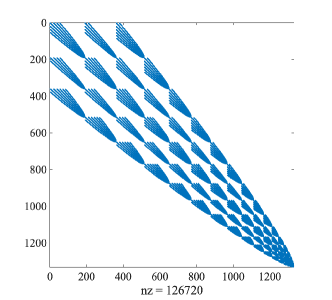
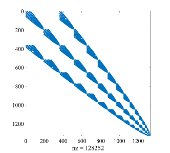
Figure 4.1: The sparse pattern of $\mathcal{S}$ (left) and $\mathcal{M}$ (right) on the reference tetrahedron when $M=22$.

Remark 4.2

Condition numbers of the stiffness matrix and the mass matrix associated with different interior bases are quite different. Without preconditioning, condition numbers of matrices generated by basis functions based on integrated Jacobi polynomials [4] and by the ones proposed by Sherwin and Karniadakis [31] grow as asymptotically as $\mathcal{O}(M^{10})$ and $\mathcal{O}(M^{7})$, respectively. While the condition number of the stiffness matrix induced by our spectral-Galerkin method only grows in $\mathcal{O}(M^{4}),$ which shares the same order with that of the diagonally preconditioned matrix as Figure 4.2 indicated.

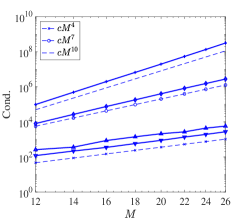
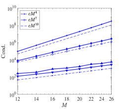
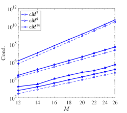
Figure 4.2: Condition numbers of ${\mathcal{S}}+{\mathcal{M}}$ (left), ${\mathcal{S}}$ (middle) and ${\mathcal{M}}$ (right) associated with different interior basis functions against $M$: $\mathcal{J}_{\bm{\ell}}$ (marked by $``\bigtriangleup"$); diagonally preconditioned (marked by $``\bigtriangledown"$); basis functions associated with integrated Jacobi polynomials (marked by $``+"$); basis functions proposed by Sherwin and Karniadakis (marked by $``\diamond"$).

4.2.3 Stiffness matrix assembling

To assemble the stiffness matrix, we need to evaluate the integral $(\nabla\varphi_{\bm{\ell}},\nabla\varphi_{\bm{k}})_{\mathcal{T}}$. Indeed, the linear mapping $\Psi$ defined in (4.1) has the following explicit form:

$$\bm{x}=\Psi(\bm{\hat{x}}):=\bm{x}^{(0)}(1-\hat{x}_{1}-\hat{x}_{2}-\hat{x}_{3})+\bm{x}^{(1)}\hat{x}_{1}+\bm{x}^{(2)}\hat{x}_{2}+\bm{x}^{(3)}\hat{x}_{3}.$$ (4.10)

It is straightforward by the chain rule in calculus that

$$\Delta =\sum\limits_{i=1}^{3}\partial_{x_{i}}^{2}=\sum\limits_{i=1}^{3}\left(\sum\limits_{j=1}^{3}\frac{\partial_{\hat{x}_{j}}}{\partial_{x_{i}}}\partial_{\hat{x}_{j}}\right)^{2}$$

$$=\sum\limits_{j=1}^{3}\left(\nabla\hat{x}_{j}\cdot\nabla\hat{x}_{j}\right)\partial_{\hat{x}_{j}}^{2}+2\sum\limits_{1\leq j<k\leq 3}\left(\nabla\hat{x}_{j}\cdot\nabla\hat{x}_{k}\right)\partial_{\hat{x}_{j}}\partial_{\hat{x}_{k}}$$

$$=\sum\limits_{j=1}^{3}\left(\nabla\hat{x}_{j}\cdot\nabla\hat{x}_{j}\right)\partial_{\hat{x}_{j}}^{2}+\sum\limits_{1\leq j<k\leq 3}\left(\nabla\hat{x}_{j}\cdot\nabla\hat{x}_{k}\right)\left(\partial^{2}_{\hat{x}_{j}}+\partial^{2}_{\hat{x}_{k}}\right)-\sum\limits_{1\leq j<k\leq 3}\left(\nabla\hat{x}_{j}\cdot\nabla\hat{x}_{k}\right)\left(\partial_{\hat{x}_{k}}-\partial_{\hat{x}_{j}}\right)^{2}$$

$$=\sum\limits_{j=1}^{3}\left(\nabla\hat{x}_{j}\cdot\nabla(\hat{x}_{1}+\hat{x}_{2}+\hat{x}_{3})\right)\partial_{\hat{x}_{j}}^{2}-\sum\limits_{1\leq j<k\leq 3}\left(\nabla\hat{x}_{j}\cdot\nabla\hat{x}_{k}\right)\left(\partial_{\hat{x}_{k}}-\partial_{\hat{x}_{j}}\right)^{2}.$$

Combining with geometric interpretation of the cross product and the triple product, it then follows from (4.10) that

$$\begin{cases}\nabla\hat{x}_{1}=\frac{(\bm{x}^{(2)}-\bm{x}^{(0)})\times(\bm{x}^{(3)}-\bm{x}^{(0)})}{(\bm{x}^{(1)}-\bm{x}^{(0)},\bm{x}^{(2)}-\bm{x}^{(0)},\bm{x}^{(3)}-\bm{x}^{(0)})}=-\frac{|F_{1}|}{3|\mathcal{T}|}\bm{n}_{1}\\[5.0pt] \nabla\hat{x}_{2}=\frac{(\bm{x}^{(3)}-\bm{x}^{(0)})\times(\bm{x}^{(1)}-\bm{x}^{(0)})}{(\bm{x}^{(1)}-\bm{x}^{(0)},\bm{x}^{(2)}-\bm{x}^{(0)},\bm{x}^{(3)}-\bm{x}^{(0)})}=-\frac{|F_{2}|}{3|\mathcal{T}|}\bm{n}_{2}\\[5.0pt] \nabla\hat{x}_{3}=\frac{(\bm{x}^{(1)}-\bm{x}^{(0)})\times(\bm{x}^{(2)}-\bm{x}^{(0)})}{(\bm{x}^{(1)}-\bm{x}^{(0)},\bm{x}^{(2)}-\bm{x}^{(0)},\bm{x}^{(3)}-\bm{x}^{(0)})}=-\frac{|F_{3}|}{3|\mathcal{T}|}\bm{n}_{3},\\[5.0pt] \nabla\left(\hat{x}_{1}+\hat{x}_{2}+\hat{x}_{3}\right)=\frac{(\bm{x}^{(2)}-\bm{x}^{(1)})\times(\bm{x}^{(3)}-\bm{x}^{(1)})}{(\bm{x}^{(1)}-\bm{x}^{(0)},\bm{x}^{(2)}-\bm{x}^{(0)},\bm{x}^{(3)}-\bm{x}^{(0)})}=\frac{|F_{0}|}{3|\mathcal{T}|}\bm{n}_{0},\end{cases}$$

where $F_{j}$ denotes the face opposite to the vertex $P_{j}$ and $\bm{n}_{j}$ is the outward normal vector of the face $F_{j}$ on the tetrahedron $\mathcal{T}$ for $0\leq j\leq 3$; $|\mathcal{T}|$ and $|F_{j}|$ stand for the volume of $\mathcal{T}$ and the area of $F_{j}$, respectively. Further let $\langle F_{j},F_{k}\rangle$ be the dihedral angle of the face $F_{j}$ and $F_{k}$. Then

$$\nabla\hat{x}_{j}\cdot\nabla(\hat{x}_{1}+\hat{x}_{2}+\hat{x}_{3})=\frac{|F_{0}||F_{j}|}{9|\mathcal{T}|^{2}}\cos\langle F_{0},F_{j}\rangle,\quad 1\leq j\leq 3,$$

$$\nabla\hat{x}_{j}\cdot\nabla\hat{x}_{k}=-\frac{|F_{j}||F_{k}|}{9|\mathcal{T}|^{2}}\cos\langle F_{j},F_{k}\rangle,\quad 1\leq j<k\leq 3,$$

since $\bm{n}_{j}\cdot\bm{n}_{k}=-\cos\langle F_{j},F_{k}\rangle$ when $j\neq k.$ Thus, the elements in the stiffness matrix are evaluated by

$$\left(\nabla{\varphi}_{\bm{\ell}},\nabla{\varphi}_{\bm{k}}\right)_{\mathcal{T}}= -\frac{2}{3|\mathcal{T}|}\,\bigg{[}\sum\limits_{j=1}^{3}|F_{0}||F_{j}|\cos\langle F_{0},F_{j}\rangle\left(\partial_{\hat{x}_{j}}\hat{\varphi}_{\bm{\ell}},\partial_{\hat{x}_{j}}\hat{\varphi}_{\bm{k}}\right)_{\hat{\mathcal{T}}}$$

$$\qquad\qquad+\sum\limits_{1\leq j<k\leq 3}|F_{j}||F_{k}|\cos\langle F_{j},F_{k}\rangle\left((\partial_{\hat{x}_{k}}-\partial_{\hat{x}_{j}})\hat{\varphi}_{\bm{\ell}},(\partial_{\hat{x}_{k}}-\partial_{\hat{x}_{j}})\hat{\varphi}_{\bm{k}}\right)_{\hat{\mathcal{T}}}\bigg{]}.$$

According to Lemma B.1 and Lemma A.1, each derivative on the reference tetrahedron $\hat{\mathcal{T}}$ is exactly a finite series of Koornwinder-Dubiner polynomials, which allows us to evaluate the accurate matrix entries by the orthogonality.

4.2.4 Mass matrix assembling

When $\gamma$ is a constant, the entries of the mass matrix could be evaluated by

$$\left({\varphi}_{\bm{\ell}},{\varphi}_{\bm{k}}\right)_{\mathcal{T}}=6\gamma|\mathcal{T}|\left(\hat{\varphi}_{\bm{\ell}},\hat{\varphi}_{\bm{k}}\right)_{\hat{\mathcal{T}}}.$$ (4.11)

Again, each $\hat{\varphi}_{\bm{\ell}}$ is a finite expansion of Koornwinder-Dubiner polynomials based on Lemma A.1 so that the integration in (4.11) could be evaluated exactly via the orthogonality.

However, when $\gamma=\gamma(x)$ is a variable coefficient, the cost in order to obtain ${\mathcal{M}}_{\gamma}$ is $\mathcal{O}(M^{9})$ by using the qualified numerical quadrature. In this subsection, we shall assemble the matrix ${\mathcal{M}}_{\gamma}$ associated with a variable coefficient recursively by making use of the three-term recurrence relation (2.22) to reduce the order of complexity to $\mathcal{O}(M^{6})$.

We first rearrange the basis polynomials $\{{\varphi}_{\bm{\ell}}\}$ with respect to the total degree in $\Phi_{M}$ where

$$\Phi_{M}=\left(\begin{array}[]{c}\bm{\varphi}_{4}\\ \bm{\varphi}_{5}\\ \vdots\\ \bm{\varphi}_{M}\end{array}\right),\quad{\text{with}}\,\,\bm{\varphi}_{m}=\left(\begin{array}[]{c}\bm{\varphi}_{m,2}\\ \bm{\varphi}_{m,3}\\ \vdots\\ \bm{\varphi}_{m,{m-2}},\end{array}\right),\quad\bm{\varphi}_{m,{k}}=\left(\begin{array}[]{c}\varphi_{k,1,m-k-1}\\ \varphi_{k,2,m-k-2}\\ \vdots\\ \varphi_{k,m-k-1,1}\end{array}\right),\quad\begin{array}[]{l}2\leq k\leq m-2,\\ 4\leq m\leq M.\end{array}$$

Then, the matrix in a block form

$$\int_{\mathcal{T}}\gamma(\bm{x})\Phi_{M}(\bm{x})\Phi_{M}(\bm{x})^{\mathsf{T}}d{\bm{x}}=\left(\begin{array}[]{ccc}H_{4,4}&\cdots&H_{4,M}\\ \vdots&\ddots&\vdots\\ H_{M,4}&\cdots&H_{M,M}\end{array}\right),$$ (4.12)

with

$$H_{m,k}=\int_{\mathcal{T}}\gamma(\bm{x}){\bm{\varphi}}_{m}(\bm{x}){{\bm{\varphi}}}_{k}(\bm{x})^{\mathsf{T}}d\bm{x},\quad 4\leq m,k\leq M,$$

could be regarded as a rearrangement of the rows and columns in the matrix ${\mathcal{M}}_{\gamma}$.

For convenience, all coefficient matrices in the three-term recurrence relation (2.22) and the generalized inverse $D_{m}$ are equally partitioned into three blocks,

$$A_{m}=\left(\begin{array}[]{c}A_{m}^{1}\\ A_{m}^{2}\\ A_{m}^{3}\end{array}\right),\quad B_{m}(\bm{x})+\left(\begin{array}[]{c}x_{1}I\\ x_{2}I\\ x_{3}I\end{array}\right)=\left(\begin{array}[]{c}B_{m}^{1}\\ B_{m}^{2}\\ B_{m}^{3}\end{array}\right),\quad C_{m}=\left(\begin{array}[]{c}C_{m}^{1}\\ C_{m}^{2}\\ C_{m}^{3}\end{array}\right),\quad D_{m}=\left(D_{m}^{1},D_{m}^{2},D_{m}^{3}\right).$$

For any integer $1\leq i\leq 3$, it is straightforward to obtain that

$$\int_{\mathcal{T}}\gamma(\bm{x})x_{i}{\bm{\varphi}}_{m}(\bm{x}){\bm{\varphi}}_{k}(\bm{x})^{\mathsf{T}}d\bm{x} =\int_{\mathcal{T}}\gamma(\bm{x})\left(C_{m}^{i}{{\bm{\varphi}}}_{m-1}(\bm{x})+B_{m}^{i}{{\bm{\varphi}}}_{m}(\bm{x})+A_{m}^{i}{{\bm{\varphi}}}_{m+1}(\bm{x})\right){{\bm{\varphi}}}_{k}(\bm{x})^{\mathsf{T}}d\bm{x}$$

$$=C_{m}^{i}H_{m-1,k}+B_{m}^{i}H_{m,k}+A_{m}^{i}H_{m+1,k}$$

$$=\int_{\mathcal{T}}\gamma(\bm{x}){{\bm{\varphi}}}_{m}(\bm{x})\left(C_{k}^{i}{{\bm{\varphi}}}_{k-1}(\bm{x})+B_{k}^{i}{{\bm{\varphi}}}_{k}(\bm{x})+A_{k}^{i}{{\bm{\varphi}}}_{k+1}(\bm{x})\right)^{\mathsf{T}}d\bm{x}$$

$$=H_{m,k-1}{C_{k}^{i\,\mathsf{T}}}+H_{m,k}B_{k}^{i\,\mathsf{T}}+H_{m,k+1}A_{k}^{i\,\mathsf{T}}.$$

As a result, it holds that

$$A_{m}^{i}H_{m+1,k}=H_{m,k-1}{C_{k}^{i\,\mathsf{T}}}+H_{m,k}B_{k}^{i\,\mathsf{T}}+H_{m,k+1}A_{k}^{i\,\mathsf{T}}-B_{m}^{i}H_{m,k}-C_{m}^{i}H_{m-1,k}.$$ (4.13)

Equivalently, one has

$$\left(\begin{array}[]{c}A_{m}^{1}\\[1.99997pt] A_{m}^{2}\\[1.99997pt] A_{m}^{3}\end{array}\right)H_{m+1,k} =\left(\begin{array}[]{c}H_{m,k-1}C_{k}^{1\,\mathsf{T}}\\[1.99997pt] H_{m,k-1}C_{k}^{2\,\mathsf{T}}\\[1.99997pt] H_{m,k-1}C_{k}^{3\,\mathsf{T}}\end{array}\right)+\left(\begin{array}[]{c}H_{m,k}B_{k}^{1\,\mathsf{T}}\\[1.99997pt] H_{m,k}B_{k}^{2\,\mathsf{T}}\\[1.99997pt] H_{m,k}B_{k}^{3\,\mathsf{T}}\end{array}\right)+\left(\begin{array}[]{c}H_{m,k+1}A_{k}^{1\,\mathsf{T}}\\[1.99997pt] H_{m,k+1}A_{k}^{2\,\mathsf{T}}\\[1.99997pt] H_{m,k+1}A_{k}^{3\,\mathsf{T}}\end{array}\right)$$

$$\qquad\quad-\left(\begin{array}[]{c}B_{m}^{1}\\[1.99997pt] B_{m}^{2}\\[1.99997pt] B_{m}^{3}\end{array}\right)H_{m,k}-\left(\begin{array}[]{c}C_{m}^{1}\\[1.99997pt] C_{m}^{2}\\[1.99997pt] C_{m}^{3}\end{array}\right)H_{m-1,k}.$$

Further recalling that $D_{m}A_{m}=I,$ we arrive at

$$H_{m+1,k} =\sum_{i=1}^{3}D_{m}^{i}H_{m,k-1}C_{k}^{i\,\mathsf{T}}+\sum_{i=1}^{3}D_{m}^{i}H_{m,k}B_{k}^{i\,\mathsf{T}}+\sum_{i=1}^{3}D_{m}^{i}H_{m,k+1}A_{k}^{i\,\mathsf{T}}$$ (4.14)

$$\,\,-\sum_{i=1}^{3}D_{m}^{i}B_{m}^{i}H_{m,k}-\sum_{i=1}^{3}D_{m}^{i}C_{m}^{i}H_{m-1,k}$$

It indicates that the block $H_{m+1,k}$ is derived by other small matrices known in previous steps. To obtain each block matrix in (4.12), one first needs to compute small blocks

$$H_{4,k}=\int_{\mathcal{T}}\gamma(\bm{x}){{\bm{\varphi}}}_{4}(\bm{x}){{\bm{\varphi}}}_{k}(\bm{x})^{\mathsf{T}}d\bm{x},\quad 4\leq k\leq 2M-4,$$

where ${{\bm{\varphi}}}_{4}$ only contains the basis function $\varphi_{2,1,1}$. As $H_{m,k}=H_{k,m}^{\mathsf{T}}$ is symmetric, one then follows (4.14) to derive the blocks

$$H_{m+1,k},\quad m+1\leq k\leq 2M-m-1,\,\,4\leq m\leq M-1.$$

With these blocks arranged as (4.12) defines, ${{\mathcal{M}}}_{\gamma}$ is consequently derived after a rearrangement.

5 Numerical experiments

To illustrate the validation of our spectral-Galerkin approximation scheme, we carry out some numerical experiments in this section.

5.1 Numerical examples for source problems

We shall present some numerical results for source problems in this subsection.

Example 5.1

Consider the second-order model equation subject to the homogeneous Dirichlet boundary condition:

$$\begin{cases}-\Delta u(\bm{x})+u(\bm{x})=f(\bm{x}),\quad&\bm{x}\in\hat{\mathcal{T}},\\ u(\bm{x})=0,\quad&\bm{x}\in\partial\hat{\mathcal{T}},\end{cases}$$ (5.1)

with the exact solution

$$u(\bm{x})=\sin\frac{\pi x_{1}}{2}\sin\frac{\pi x_{2}}{2}\sin\frac{\pi x_{3}}{2}\sin\frac{\pi(1-x_{1}-x_{2}-x_{3})}{2}.$$ (5.2)

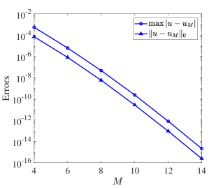
Figure 5.1: Maximum pointwise errors and $L^{2}$-errors against $M$ in Example 5.1 (left) and Example 5.2 (right).

Owing to the homogeneous Dirichlet boundary, only interior modes of polynomial basis functions are involved in our numerical scheme. It is observed in the left of Figure 5.1 that both maximum pointwise errors and $L^{2}$-errors of $u-u_{M}$ decay exponentially, which verifies the effectiveness and spectral accuracy of our spectral-Galerkin method.

Example 5.2

Consider the Poisson equation subject to the non-homogeneous Dirichlet boundary condition:

$$\begin{cases}-\Delta u(\bm{x})=f(\bm{x}),\quad&\bm{x}\in\hat{\mathcal{T}},\\ u(\bm{x})=g(\bm{x}),\quad&\bm{x}\in\partial\hat{\mathcal{T}},\end{cases}$$ (5.3)

with the exact solution

$$u(\bm{x})=(x_{1}+1)(x_{2}+1)(x_{3}+1)e^{1-x_{1}-x_{2}-x_{3}}.$$

It follows from the right of Figure 5.1 that the numerical scheme (4.4) achieves exponential orders of convergence for the second-order model problem with the non-homogeneous Dirichlet boundary condition, which confirms the spectral accuracy on the approximation of the solution along boundaries.

Example 5.3

Consider the second-order model equation subject to the homogeneous Dirichlet boundary condition:

$$\begin{cases}-\Delta u(\bm{x})+\gamma(\bm{x})u(\bm{x})=f(\bm{x}),\quad&\bm{x}\in\hat{\mathcal{T}},\\ u(\bm{x})=0,\quad&\bm{x}\in\partial\hat{\mathcal{T}},\end{cases}$$ (5.4)

with the exact solution defined as in (5.2) and a variable coefficient

$$\gamma(\bm{x})=e^{x_{1}+x_{2}+x_{3}+1}.$$

Exponential orders of convergence of errors $u-u_{M}$ in the maximum pointwise errors and $L^{2}$-errors are also observed from the semi-log graph in Figure 5.2. This reflect the effectiveness of our method for solving equations with non-homogeneous boundary conditions.

Figure 5.2: Maximum pointwise errors and $L^{2}$-errors against $M$ in Example 5.3.

Example 5.4

Consider the heat equation subject to the homogeneous Dirichlet boundary condition:

$$\begin{cases}\partial_{t}u(\bm{x},t)-\Delta u(\bm{x},t)=f(\bm{x},t),\quad&(\bm{x},t)\in\hat{\mathcal{T}}\times(0,T],\\ u(\bm{x},t)=0,\quad&(\bm{x},t)\in\partial\hat{\mathcal{T}}\times(0,T],\\ u(\bm{x},0)=u_{0}(\bm{x}),\quad&\bm{x}\in\hat{\mathcal{T}},\end{cases}$$ (5.5)

with $T=1$ and the exact solution

$$u(\bm{x},t)=\sin\pi x_{1}\sin\pi x_{2}\sin\pi x_{3}\sin\pi(1-x_{1}-x_{2}-x_{3})e^{-t}.$$

We use the Crank-Nicolson method [7] to design the fully discretization scheme. Let

$$0=t_{0}<t_{1}<\cdots<t_{N}=T,\quad N\in\mathbb{N},$$

be the discrete partition in time. We further let $\Delta t$ be the time-step and $t_{n}=n\Delta t$ be the $n$-th time-level. The values of the approximation solution $u_{M}$ and the right-hand side function $f$ at time-step $n$ are denoted by $u_{M}^{n}$ and $f^{n},$ respectively. Combining with (4.4), the fully discretization scheme of (5.5) reads: for all $0\leq n\leq N,$ to find $u_{M}^{n}\in X_{M,0}$ such that

$$\left(\frac{u^{n+1}_{M}-u^{n}_{M}}{\Delta t},v_{M}\right)_{\hat{\mathcal{T}}}+a\left(\frac{u_{M}^{n+1}+u_{M}^{n}}{2},v_{M}\right)=\left(\frac{f^{n+1}+f^{n}}{2},v_{M}\right)_{\hat{\mathcal{T}}},\quad\forall v_{M}\in X_{M,0}.$$ (5.6)

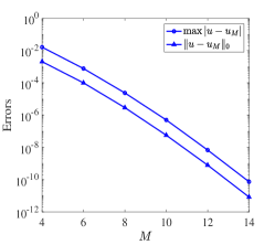
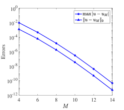
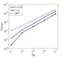
Figure 5.3: Maximum pointwise errors and $L^{2}$-errors against $M$ when $t=1/2$ (left) and $t=1$ (middle); $L^{2}$-errors against $\Delta t$ (right) in Example 5.4.

Setting $\Delta t=2^{-14}$, we first demonstrate errors of $u-u_{M}$ against $M$ in different time in Figure 5.3. It is reported that the errors decay exponentially both when $t=1/2$ and $t=1$. Letting $M=14,$ we also observe from the right of Figure 5.3 that the Crank-Nicolson scheme has second-order convergence in time.

5.2 Numerical examples for eigenvalue problems

We report the numerical results for the Laplacian eigenvalue problem (4.5) in this subsection. Two special tetrahedra would be considered in the following discussions: the fundamental tetrahedron $\mathcal{T}_{F}$ with vertices

$$P^{F}_{0}=\left(0,0,0\right)^{\mathsf{T}},\quad P^{F}_{1}=\left(0,0,1\right)^{\mathsf{T}},\quad P^{F}_{2}=\left(\frac{1}{2},\frac{1}{2},\frac{1}{2}\right)^{\mathsf{T}},\quad P^{F}_{3}=\left(-\frac{1}{2},\frac{1}{2},\frac{1}{2}\right)^{\mathsf{T}},$$

and the regular tetrahedron $\mathcal{T}_{R}$ with vertices

$$P^{R}_{0}=\left(0,0,\frac{\sqrt{6}}{3}\right)^{\mathsf{T}},\quad P^{R}_{1}=\left(\frac{\sqrt{3}}{3},0,0\right)^{\mathsf{T}},\quad P^{R}_{2}=\left(-\frac{\sqrt{3}}{6},\frac{1}{2},0\right)^{\mathsf{T}},\quad P^{R}_{3}=\left(-\frac{\sqrt{3}}{6},-\frac{1}{2},0\right)^{\mathsf{T}}.$$

All eigenvalues of the homogeneous Dirichlet Laplacian can be arranged as

$$0<\mu_{1}<\mu_{2}\leq\mu_{3}\leq\cdots\leq\mu_{k}\leq\cdots,\quad k\in\mathbb{N}.$$

To begin with, we test absolute errors when approximating the five smallest eigenvalues by numerical scheme (4.7) on two tetrahedra. For $\mathcal{T}_{F}$, the exact eigenvalues are obtained in Appendix D; while for $\mathcal{T}_{R}$, the reference eigenvalues are derived with relatively large $M$ by our spectral-Galerkin method. The semi-log and log-log graphs in Figure 5.4 reveal that the scheme achieves exponential orders of convergence on $\mathcal{T}_{F}$ and algebraic orders of convergence on $\mathcal{T}_{R}$, respectively. It means that the corresponding eigenfunctions on the regular tetrahedron would have singularities, which is quite different from the behaviors of eigenfunctions on the regular triangle. Indeed, the Laplacian eigenfunctions associated with the first few eigenvalues on the regular triangle are analytic [26, 23] and the polynomial spectral method achieves exponential orders of convergence when approximating these eigen-solutions [27].

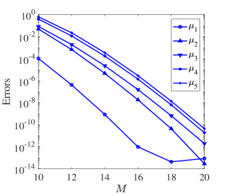
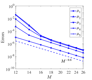
Figure 5.4: Absolute errors of the five smallest numerical Laplacian eigenvalues against $M$ on $\mathcal{T}_{F}$ (left) and $\mathcal{T}_{R}$ (right).

We then move on to study the approximations on large eigenvalues. The Weyl’s Conjecture in three dimensions [33, 15] reads that,

$$\mu_{k}=\frac{\pi(36\pi)^{\frac{1}{3}}}{|\mathcal{T}|^{\frac{2}{3}}}k^{\frac{2}{3}}+\frac{\pi}{2}\left(\frac{3\pi^{2}}{4}\right)^{\frac{1}{3}}\frac{|\partial\mathcal{T}|}{|\mathcal{T}|^{\frac{4}{3}}}k^{\frac{1}{3}}+o(k^{\frac{1}{3}}),\quad k\rightarrow+\infty,$$ (5.7)

where $|\mathcal{T}|$ and $|\partial\mathcal{T}|$ represent the volume and surface area of $\mathcal{T}$, respectively. Thus, the exact eigenvalue $\mu_{k}$, $k=\mathcal{O}(M^{3})$, grows in $\mathcal{O}(M^{2})$ as $M$ tends to $\infty$. However, we observe in Figure 5.5 that the largest numerical eigenvalue $\mu_{M,\frac{(M-1)(M-2)(M-3)}{6}}$ evaluated by our spectral-Galerkin method with different $M$ grows almost as asymptotically as $\mathcal{O}(M^{4})$. It indicates that the polynomial spectral method would bring out a portion of spurious solutions in deriving large numerical eigenvalues.

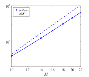
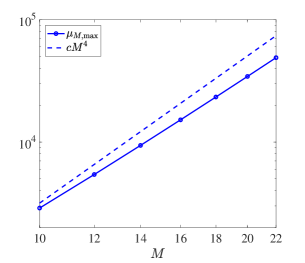
Figure 5.5: The largest numerical Laplacian eigenvalue against $M$ on $\mathcal{T}_{F}$ (left) and $\mathcal{T}_{R}$ (right).

As a result, one should check how many reliable eigen-solutions that our method is able to provide before examining asymptotic properties of large eigenvalues. We understand reliable to mean at least $\mathcal{O}(M^{-1})$ accuracy with polynomial degree $M$. With exact eigenvalues known in Appendix D, we solve the generalized eigenvalue problem (4.7) on $\mathcal{T}_{F}$ with different values of $M$ and illustrate their relative errors in the left and the middle of Figure 5.6.

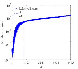
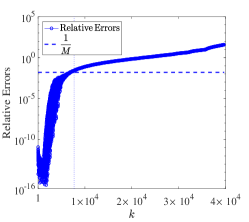
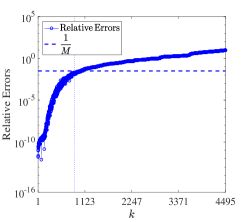
Figure 5.6: Relatives errors of all numerical eigenvalues on $\mathcal{T}_{F}$ when $M=32$ (left) and $M=64$ (middle); on $\mathcal{T}_{R}$ when $M=32$ (right). The vertical dashed line denotes the portion of $\frac{3}{4}(\frac{2}{\pi})^{3}.$

It follows that there are about $\frac{3}{4}(\frac{2}{\pi})^{3}\approx 19.35\%$ numerical eigenvalues for which relative errors converge at rate $\mathcal{O}(M^{-1})$ for our spectral-Galerkin method. Referred by eigenvalues derived with relatively large $M$, we also draw convergence behaviors of numerical eigenvalues on $\mathcal{T}_{R}$ when $M=32$ in the right of Figure 5.6. Although none of our numerical eigenvalues can reach the machine precision in this case, almost same portion of reliable eigenvalues are observed.

Now, let us demonstrate in Figure 5.7 the asymptotic behaviors of the first reliable 3000 numerical eigenvalues of (4.7) computed by our spectral method with $M=64$. We observe that numerical eigenvalues suit well with the Weyl’s conjecture (5.7). It, in return, confirms once again the accuracy of these numerical eigenvalues.

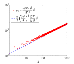
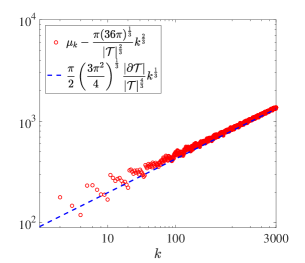
Figure 5.7: Asymptotic behaviors of eigenvalues $\mu_{k}$ against $k$ on $\mathcal{T}_{F}$ (left) and $\mathcal{T}_{R}$ (right).

Next, we turn to explore different gaps of these reliable numerical eigenvalues. We introduce the following definitions [16, 3]:

• the average gaps:   $\delta_{\rm ave}(k):=\dfrac{1}{k}\sum\limits_{j=1}^{k}\left(\mu_{j+1}-\mu_{j}\right)=\dfrac{\mu_{k+1}-\mu_{1}}{k},\,k\in\mathbb{N};$

• the normalized gaps:   $\delta_{\rm norm}(k):=y_{k+1}-y_{k},\,$ $y_{k}=\left(\mu_{k}\cdot\frac{|\mathcal{T}|^{\frac{2}{3}}}{\pi(36\pi)^{\frac{1}{3}}}\right)^{3/2}$,  $k\in\mathbb{N}$.

Another interesting term is the level spacing distribution $P(s)$ representing the limiting distribution of the normalized gaps, which is defined by [16, 3]

$$\dfrac{\sharp\{j\,|1\leq j\leq k\,|\,\delta_{\rm norm}(j)<x\}}{k}\stackrel{{\scriptstyle k\rightarrow+\infty}}{{\longrightarrow}}\int_{0}^{x}P(s)\,ds,\quad 0\leq x<+\infty,$$

where $\sharp S$ denotes the cardinality of the set $S$.

For both $\mathcal{T}_{F}$ and $\mathcal{T}_{R}$, similar observations are derived from Figure 5.8 and Figure 5.9: $\delta_{\rm ave}(k)\sim k^{-\frac{1}{3}}$, which is also a direct consequence of (5.7) and the definition of $\delta_{\rm ave}(k)$; statistically, the gaps distribution satisfies $P(s)=\delta(s)$, where $\delta(s)$ is the Dirac delta function.

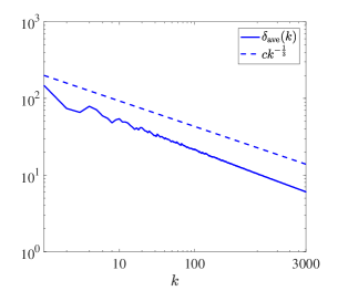
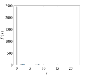
Figure 5.8: The average gaps (left) and the level spacing distribution (right) on $\mathcal{T}_{F}$.

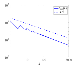
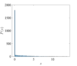
Figure 5.9: The average gaps (left) and the level spacing distribution (right) on $\mathcal{T}_{R}$.

6 Conclusion

We introduced in this paper a sparse spectral-Galerkin method for second-order partial differential equations on an arbitrary tetrahedron using generalized Koornwinder polynomials. By exploring various recurrence relations of generalized Koornwinder polynomials, we derive well-conditioned and sparse linear systems which can be efficiently solved. Numerical results for different kinds of source problems and the Laplacian eigenvalue problem confirm the sparsity, effectiveness and spectral accuracy of our method.

With the modal basis functions defined in this paper being applied directly for $C^{0}$-conforming elements, this work can be instantly extended to spectral-element methods on tetrahedral meshes for complex geometries. Theoretical approximation results will also be investigated in a future work.

Appendix A Recurrence relations for increasing parameters

We derive some useful recurrence relations for generalized Koornwinder polynomials in Appendix A-B. Firstly, we rewrite the Koornwinder polynomials in the collapsed coordinate to simplify the incoming proofs,

$$\mathcal{J}_{\bm{\ell}}^{\bm{\alpha}}(\bm{\hat{x}})=J_{\ell_{1}}^{\alpha_{0},\alpha_{1}}(\xi)\left(\frac{1-\eta}{2}\right)^{\ell_{1}}J_{\ell_{2}}^{2\ell_{1}+\alpha_{0}+\alpha_{1}+1,\alpha_{2}}(\eta)\left(\frac{1-\zeta}{2}\right)^{\ell_{1}+\ell_{2}}J_{\ell_{3}}^{2\ell_{1}+2\ell_{2}+\alpha_{0}+\alpha_{1}+\alpha_{2}+2,\alpha_{3}}(\zeta),$$ (A.1)

where

$$\xi=\dfrac{2\hat{x}_{1}}{1-\hat{x}_{2}-\hat{x}_{3}}-1,\quad\eta=\dfrac{2\hat{x}_{2}}{1-\hat{x}_{3}}-1,\quad\zeta=2\hat{x}_{3}-1.$$ (A.2)

We also let

$$\dot{\bm{e}}_{0}=(1,0,0,0),\quad\dot{\bm{e}}_{1}=(0,1,0,0),\quad\dot{\bm{e}}_{2}=(0,0,1,0),\quad\dot{\bm{e}}_{3}=(0,0,0,1).$$

All coefficient functions in appendixes are defined as in Lemma 2.1-2.4.

Lemma A.1

For any $\bm{\alpha}\in[-1,+\infty)^{4}$ and $\bm{\ell}\in\mathbb{N}_{0}^{3}$, the following recurrence relations hold:

$${\mathcal{J}}_{\bm{\ell}}^{\bm{\alpha}}(\bm{\hat{x}})=\sum\limits_{p=0}^{1}\sum\limits_{q=0}^{1}\sum\limits_{r=0}^{1}\mathcal{A}_{p,q,r}^{1}(\bm{\ell},\bm{\alpha}){\mathcal{J}}_{\bm{\ell}-\left(p,\,q-p,\,r-q\right)}^{{\bm{\alpha}}+\dot{\bm{e}}_{0}}(\bm{\hat{x}}),$$ (A.3)

$${\mathcal{J}}_{\bm{\ell}}^{\bm{\alpha}}(\bm{\hat{x}})=\sum\limits_{p=0}^{1}\sum\limits_{q=0}^{1}\sum\limits_{r=0}^{1}\mathcal{A}_{p,q,r}^{2}(\bm{\ell},\bm{\alpha}){\mathcal{J}}_{\bm{\ell}-\left(p,\,q-p,\,r-q\right)}^{{\bm{\alpha}}+\dot{\bm{e}}_{1}}(\bm{\hat{x}}),$$ (A.4)

$${\mathcal{J}}_{\bm{\ell}}^{\bm{\alpha}}(\bm{\hat{x}})=\sum\limits_{q=0}^{1}\sum\limits_{r=0}^{1}\mathcal{A}_{q,r}^{3}(\bm{\ell},\bm{\alpha}){\mathcal{J}}_{\bm{\ell}-\left(0,\,q,\,r-q\right)}^{{\bm{\alpha}}+\dot{\bm{e}}_{2}}(\bm{\hat{x}}),$$ (A.5)

$${\mathcal{J}}_{\bm{\ell}}^{\bm{\alpha}}(\bm{\hat{x}})=\sum\limits_{r=0}^{1}\mathcal{A}_{r}^{4}(\bm{\ell},\bm{\alpha}){\mathcal{J}}_{\bm{\ell}-\left(0,0,r\right)}^{{\bm{\alpha}}+\dot{\bm{e}}_{3}}(\bm{\hat{x}}),$$ (A.6)

where the corresponding coefficients are presented in Table A.1.

Table A.1: The values of $\mathcal{A}^{1}_{p,q,r},$ $\mathcal{A}^{2}_{p,q,r}$, $\mathcal{A}^{3}_{q,r}$ and $\mathcal{A}^{4}_{r}$.

$(p,q,r)$ $\mathcal{A}^{1}_{p,q,r}(\bm{\ell},\bm{\alpha})$ $(p,q,r)$ $\mathcal{A}^{2}_{p,q,r}(\bm{\ell},\bm{\alpha})$ (0,0,0) $b_{1,\ell_{1}}^{\alpha_{0},\alpha_{1}}b_{1,\ell_{2}}^{2\ell_{1}+|\bm{\alpha}^{1}|+1,\alpha_{2}}b_{1,\ell_{3}}^{2|\bm{\ell}^{2}|+|\bm{\alpha}^{2}|+2,\alpha_{3}}$ (0,0,0) $b_{1,\ell_{1}}^{\alpha_{0},\alpha_{1}}b_{1,\ell_{2}}^{2\ell_{1}+|\bm{\alpha}^{1}|+1,\alpha_{2}}b_{1,\ell_{3}}^{2|\bm{\ell}^{2}|+|\bm{\alpha}^{2}|+2,\alpha_{3}}$ (0,0,1) $b_{1,\ell_{1}}^{\alpha_{0},\alpha_{1}}b_{1,\ell_{2}}^{2\ell_{1}+|\bm{\alpha}^{1}|+1,\alpha_{2}}b_{2,\ell_{3}}^{2|\bm{\ell}^{2}|+|\bm{\alpha}^{2}|+2,\alpha_{3}}$ (0,0,1) $b_{1,\ell_{1}}^{\alpha_{0},\alpha_{1}}b_{1,\ell_{2}}^{2\ell_{1}+|\bm{\alpha}^{1}|+1,\alpha_{2}}b_{2,\ell_{3}}^{2|\bm{\ell}^{2}|+|\bm{\alpha}^{2}|+2,\alpha_{3}}$ (0,1,0) $b_{1,\ell_{1}}^{\alpha_{0},\alpha_{1}}b_{2,\ell_{2}}^{2\ell_{1}+|\bm{\alpha}^{1}|+1,\alpha_{2}}e_{2,\ell_{3}}^{2|\bm{\ell}^{2}|+|\bm{\alpha}^{2}|+1,\alpha_{3}}$ (0,1,0) $b_{1,\ell_{1}}^{\alpha_{0},\alpha_{1}}b_{2,\ell_{2}}^{2\ell_{1}+|\bm{\alpha}^{1}|+1,\alpha_{2}}e_{2,\ell_{3}}^{2|\bm{\ell}^{2}|+|\bm{\alpha}^{2}|+1,\alpha_{3}}$ (0,1,1) $b_{1,\ell_{1}}^{\alpha_{0},\alpha_{1}}b_{2,\ell_{2}}^{2\ell_{1}+|\bm{\alpha}^{1}|+1,\alpha_{2}}e_{1,\ell_{3}}^{2|\bm{\ell}^{2}|+|\bm{\alpha}^{2}|+1,\alpha_{3}}$ (0,1,1) $b_{1,\ell_{1}}^{\alpha_{0},\alpha_{1}}b_{2,\ell_{2}}^{2\ell_{1}+|\bm{\alpha}^{1}|+1,\alpha_{2}}e_{1,\ell_{3}}^{2|\bm{\ell}^{2}|+|\bm{\alpha}^{2}|+1,\alpha_{3}}$ (1,0,0) $b_{2,\ell_{1}}^{\alpha_{0},\alpha_{1}}e_{2,\ell_{2}}^{2\ell_{1}+|\bm{\alpha}^{1}|,\alpha_{2}}b_{1,\ell_{3}}^{2|\bm{\ell}^{2}|+|\bm{\alpha}^{2}|+2,\alpha_{3}}$ (1,0,0) $-b_{2,\ell_{1}}^{\alpha_{1},\alpha_{0}}e_{2,\ell_{2}}^{2\ell_{1}+|\bm{\alpha}^{1}|,\alpha_{2}}b_{1,\ell_{3}}^{2|\bm{\ell}^{2}|+|\bm{\alpha}^{2}|+2,\alpha_{3}}$ (1,0,1) $b_{2,\ell_{1}}^{\alpha_{0},\alpha_{1}}e_{2,\ell_{2}}^{2\ell_{1}+|\bm{\alpha}^{1}|,\alpha_{2}}b_{2,\ell_{3}}^{2|\bm{\ell}^{2}|+|\bm{\alpha}^{2}|+2,\alpha_{3}}$ (1,0,1) $-b_{2,\ell_{1}}^{\alpha_{1},\alpha_{0}}e_{2,\ell_{2}}^{2\ell_{1}+|\bm{\alpha}^{1}|,\alpha_{2}}b_{2,\ell_{3}}^{2|\bm{\ell}^{2}|+|\bm{\alpha}^{2}|+2,\alpha_{3}}$ (1,1,0) $b_{2,\ell_{1}}^{\alpha_{0},\alpha_{1}}e_{1,\ell_{2}}^{2\ell_{1}+|\bm{\alpha}^{1}|,\alpha_{2}}e_{2,\ell_{3}}^{2|\bm{\ell}^{2}|+|\bm{\alpha}^{2}|+1,\alpha_{3}}$ (1,1,0) $-b_{2,\ell_{1}}^{\alpha_{1},\alpha_{0}}e_{1,\ell_{2}}^{2\ell_{1}+|\bm{\alpha}^{1}|,\alpha_{2}}e_{2,\ell_{3}}^{2|\bm{\ell}^{2}|+|\bm{\alpha}^{2}|+1,\alpha_{3}}$ (1,1,1) $b_{2,\ell_{1}}^{\alpha_{0},\alpha_{1}}e_{1,\ell_{2}}^{2\ell_{1}+|\bm{\alpha}^{1}|,\alpha_{2}}e_{1,\ell_{3}}^{2|\bm{\ell}^{2}|+|\bm{\alpha}^{2}|+1,\alpha_{3}}$ (1,1,1) $-b_{2,\ell_{1}}^{\alpha_{1},\alpha_{0}}e_{1,\ell_{2}}^{2\ell_{1}+|\bm{\alpha}^{1}|,\alpha_{2}}e_{1,\ell_{3}}^{2|\bm{\ell}^{2}|+|\bm{\alpha}^{2}|+1,\alpha_{3}}$ $(q,r)$ $\mathcal{A}^{3}_{q,r}(\bm{\ell},\bm{\alpha})$ $(q,r)$ $\mathcal{A}^{3}_{q,r}(\bm{\ell},\bm{\alpha})$ (0,0) $b_{1,\ell_{2}}^{2\ell_{1}+|\bm{\alpha}^{1}|+1,\alpha_{2}}b_{1,\ell_{3}}^{2|\bm{\ell}^{2}|+|\bm{\alpha}^{2}|+2,\alpha_{3}}$ (1,0) $-b_{2,\ell_{2}}^{\alpha_{2},2\ell_{1}+|\bm{\alpha}^{1}|+1}e_{2,\ell_{3}}^{2|\bm{\ell}^{2}|+|\bm{\alpha}^{2}|+1,\alpha_{3}}$ (0,1) $b_{1,\ell_{2}}^{2\ell_{1}+|\bm{\alpha}^{1}|+1,\alpha_{2}}b_{2,\ell_{3}}^{2|\bm{\ell}^{2}|+|\bm{\alpha}^{2}|+2,\alpha_{3}}$ (1,1) $-b_{2,\ell_{2}}^{\alpha_{2},2\ell_{1}+|\bm{\alpha}^{1}|+1}e_{1,\ell_{3}}^{2|\bm{\ell}^{2}|+|\bm{\alpha}^{2}|+1,\alpha_{3}}$ $r$ $\mathcal{A}^{4}_{r}(\bm{\ell},\bm{\alpha})$ $r$ $\mathcal{A}^{4}_{r}(\bm{\ell},\bm{\alpha})$ 0 $b_{1,\ell_{3}}^{2|\bm{\ell}^{2}|+|\bm{\alpha}^{2}|+2,\alpha_{3}}$ 1 $-b_{2,\ell_{3}}^{\alpha_{3},2|\bm{\ell}^{2}|+|\bm{\alpha}^{2}|+2}$

Proof  We take the proof of (A.5) as an example. Other identities shall be proved in a similar way. According to (2.9), (2.8) and (2.11), one has

$$\mathcal{J}_{\bm{\ell}}^{\bm{\alpha}}(\bm{\hat{x}}) =J_{\ell_{1}}^{\alpha_{0},\alpha_{1}}(\xi)\left(\frac{1-\eta}{2}\right)^{\ell_{1}}\bigg{[}b_{1,\ell_{2}}^{2\ell_{1}+|\bm{\alpha}^{1}|+1,\alpha_{2}}J_{\ell_{2}}^{2\ell_{1}+|\bm{\alpha}^{1}|+1,\alpha_{2}+1}(\eta)\left(\frac{1-\zeta}{2}\right)^{\ell_{1}+\ell_{2}}$$

$$\qquad\times\left(b_{1,\ell_{3}}^{2|\bm{\ell}^{2}|+|\bm{\alpha}^{2}|+2,\alpha_{3}}J_{\ell_{3}}^{2|\bm{\ell}^{2}|+|\bm{\alpha}^{2}|+3,\alpha_{3}}(\zeta)+b_{2,\ell_{3}}^{2|\bm{\ell}^{2}|+|\bm{\alpha}^{2}|+2,\alpha_{3}}J_{\ell_{3}-1}^{2|\bm{\ell}^{2}|+|\bm{\alpha}^{2}|+3,\alpha_{3}}(\zeta)\right)$$

$$\qquad\qquad-b_{2,\ell_{2}}^{\alpha_{2},2\ell_{1}+|\bm{\alpha}^{1}|+1}J_{\ell_{2}-1}^{2\ell_{1}+|\bm{\alpha}^{1}|+1,\alpha_{2}+1}(\eta)\left(\frac{1-\zeta}{2}\right)^{\ell_{1}+\ell_{2}-1}$$

$$\qquad\times\left(e_{1,\ell_{3}}^{2|\bm{\ell}^{2}|+|\bm{\alpha}^{2}|+1,\alpha_{3}}J_{\ell_{3}}^{2|\bm{\ell}^{2}|+|\bm{\alpha}^{2}|+1,\alpha_{3}}(\zeta)+e_{2,\ell_{3}}^{2|\bm{\ell}^{2}|+|\bm{\alpha}^{2}|+1,\alpha_{3}}J_{\ell_{3}+1}^{2|\bm{\ell}^{2}|+|\bm{\alpha}^{2}|+1,\alpha_{3}}(\zeta)\right)\bigg{]}.$$

This completes the proof. $\square$

Appendix B Recurrence relations for derivatives

Lemma B.1

For any $\bm{\alpha}\in[-1,+\infty)^{4}$ and $\bm{\ell}\in\mathbb{N}_{0}^{3}$, the following recurrence relations hold:

$$\partial_{\hat{x}_{1}}{\mathcal{J}}_{\bm{\ell}}^{\bm{\alpha}}(\bm{\hat{x}})=2d_{\ell_{1}}^{\alpha_{0},\alpha_{1}}{\mathcal{J}}_{\bm{\ell}-(1,0,0)}^{\bm{\alpha}+\dot{\bm{e}}_{0}+\dot{\bm{e}}_{1}}(\bm{\hat{x}}),$$ (B.1)

$$\partial_{\hat{x}_{2}}{\mathcal{J}}_{\bm{\ell}}^{\bm{\alpha}}(\bm{\hat{x}})=\sum\limits_{p=0}^{1}\mathcal{D}^{2}_{p}(\bm{\ell},\bm{\alpha}){\mathcal{J}}_{\bm{\ell}-\left(p,1-p,0\right)}^{{\bm{\alpha}}+\dot{\bm{e}}_{0}+\dot{\bm{e}}_{2}}(\bm{\hat{x}}),$$ (B.2)

$$\left(\partial_{\hat{x}_{2}}-\partial_{\hat{x}_{1}}\right){\mathcal{J}}_{\bm{\ell}}^{\bm{\alpha}}(\bm{\hat{x}})=\sum\limits_{p=0}^{1}\mathcal{D}^{21}_{p}(\bm{\ell},\bm{\alpha}){\mathcal{J}}_{\bm{\ell}-\left(p,1-p,0\right)}^{{\bm{\alpha}}+\dot{\bm{e}}_{1}+\dot{\bm{e}}_{2}}(\bm{\hat{x}}),$$ (B.3)

$$\partial_{\hat{x}_{3}}{\mathcal{J}}_{\bm{\ell}}^{\bm{\alpha}}(\bm{\hat{x}})=\sum\limits_{p=0}^{1}\sum\limits_{q=0}^{1}\mathcal{D}^{3}_{p,q}(\bm{\ell},\bm{\alpha}){\mathcal{J}}_{\bm{\ell}-\left(p,\,q-p,\,1-q\right)}^{{\bm{\alpha}}+\dot{\bm{e}}_{0}+\dot{\bm{e}}_{3}}(\bm{\hat{x}}),$$ (B.4)

$$\left(\partial_{\hat{x}_{1}}-\partial_{\hat{x}_{3}}\right){\mathcal{J}}_{\bm{\ell}}^{\bm{\alpha}}(\bm{\hat{x}})=\sum\limits_{p=0}^{1}\sum\limits_{q=0}^{1}\mathcal{D}^{13}_{p,q}(\bm{\ell},\bm{\alpha}){\mathcal{J}}_{\bm{\ell}-\left(p,\,q-p,\,1-q\right)}^{{\bm{\alpha}}+\dot{\bm{e}}_{1}+\dot{\bm{e}}_{3}}(\bm{\hat{x}}),$$ (B.5)

$$\left(\partial_{\hat{x}_{3}}-\partial_{\hat{x}_{2}}\right){\mathcal{J}}_{\bm{\ell}}^{\bm{\alpha}}(\bm{\hat{x}})=\sum\limits_{q=0}^{1}\mathcal{D}_{q}^{32}(\bm{\ell},\bm{\alpha}){\mathcal{J}}_{\bm{\ell}-\left(0,q,1-q\right)}^{{\bm{\alpha}}+\dot{\bm{e}}_{2}+\dot{\bm{e}}_{3}}(\bm{\hat{x}}).$$ (B.6)

With the notations

$$\rho_{\bm{\ell}}^{\bm{\alpha}}:=2d_{\ell_{1}}^{\alpha_{0},\alpha_{1}}e_{1,\ell_{1}-1}^{\alpha_{1},\alpha_{0}+1}-\ell_{1}b_{2,\ell_{1}}^{\alpha_{0},\alpha_{1}},\quad\kappa_{\bm{\ell}}^{\bm{\alpha}}:=\ell_{1}b_{2,\ell_{1}}^{\alpha_{1},\alpha_{0}}-2d_{\ell_{1}}^{\alpha_{0},\alpha_{1}}e_{1,\ell_{1}-1}^{\alpha_{0},\alpha_{1}+1},$$

$$\theta_{\bm{\ell}}^{\bm{\alpha}}:=2d_{\ell_{2}}^{2\ell_{1}+|\bm{\alpha}^{1}|+1,\alpha_{2}}e_{1,\ell_{2}-1}^{\alpha_{2},2\ell_{1}+|\bm{\alpha}^{1}|+2}-\ell_{2}b_{2,\ell_{2}}^{2\ell_{1}+|\bm{\alpha}^{1}|+1,\alpha_{2}},$$

the corresponding coefficients are presented as follows.

$$\mathcal{D}_{0}^{2}(\bm{\ell},\bm{\alpha})=2d_{\ell_{2}}^{2\ell_{1}+|\bm{\alpha}^{1}|+1,\alpha_{2}}b_{1,\ell_{1}}^{\alpha_{0},\alpha_{1}},$$

$$\mathcal{D}_{1}^{2}(\bm{\ell},\bm{\alpha})=\tfrac{\left(2d_{\ell_{1}}^{\alpha_{0},\alpha_{1}}e_{1,\ell_{1}-1}^{\alpha_{1},\alpha_{0}+1}-\ell_{1}b_{2,\ell_{1}}^{\alpha_{0},\alpha_{1}}\right)b_{1,\ell_{2}}^{2\ell_{1}+|\bm{\alpha}^{1}|+1,\alpha_{2}}+2d_{\ell_{2}}^{2\ell_{1}+|\bm{\alpha}^{1}|+1,\alpha_{2}}b_{2,\ell_{1}}^{\alpha_{0},\alpha_{1}}e_{2,\ell_{2}-1}^{2\ell_{1}+|\bm{\alpha}^{1}|+1,\alpha_{2}+1}}{b_{1,\ell_{2}}^{2\ell_{1}+|\bm{\alpha}^{1}|,\alpha_{2}+1}}.$$

$$\mathcal{D}_{0}^{21}(\bm{\ell},\bm{\alpha})=\mathcal{D}_{0}^{2}(\bm{\ell},\bm{\alpha}),$$

$$\mathcal{D}_{1}^{21}(\bm{\ell},\bm{\alpha})=\tfrac{\left(\ell_{1}b_{2,\ell_{1}}^{\alpha_{1},\alpha_{0}}-2d_{\ell_{1}}^{\alpha_{0},\alpha_{1}}e_{1,\ell_{1}-1}^{\alpha_{0},\alpha_{1}+1}\right)b_{1,\ell_{2}}^{2\ell_{1}+|\bm{\alpha}^{1}|+1,\alpha_{2}}-2d_{\ell_{2}}^{2\ell_{1}+|\bm{\alpha}^{1}|+1,\alpha_{2}}b_{2,\ell_{1}}^{\alpha_{1},\alpha_{0}}e_{2,\ell_{2}-1}^{2\ell_{1}+|\bm{\alpha}^{1}|+1,\alpha_{2}+1}}{b_{1,\ell_{2}}^{2\ell_{1}+|\bm{\alpha}^{1}|,\alpha_{2}+1}}.$$

$$\mathcal{D}^{3}_{0,0}(\bm{\ell},\bm{\alpha})=2d_{\ell_{3}}^{2|\bm{\ell}^{2}|+|\bm{\alpha}^{2}|+2,\alpha_{3}}b_{1,\ell_{1}}^{\alpha_{0},\alpha_{1}}b_{1,\ell_{2}}^{2\ell_{1}+|\bm{\alpha}^{1}|+1,\alpha_{2}},$$

$$\mathcal{D}^{3}_{0,1}(\bm{\ell},\bm{\alpha})=\tfrac{b_{1,\ell_{1}}^{\alpha_{0},\alpha_{1}}\theta_{\bm{\ell}}^{\bm{\alpha}}b_{1,\ell_{3}}^{2|\bm{\ell}^{2}|+|\bm{\alpha}^{2}|+2,\alpha_{3}}+2d_{\ell_{3}}^{2|\bm{\ell}^{2}|+|\bm{\alpha}^{2}|+2,\alpha_{3}}b_{1,\ell_{1}}^{\alpha_{0},\alpha_{1}}b_{2,\ell_{2}}^{2\ell_{1}+|\bm{\alpha}^{1}|+1,\alpha_{2}}e_{2,\ell_{3}-1}^{2|\bm{\ell}^{2}|+|\bm{\alpha}^{2}|+2,\alpha_{3}+1}}{b_{1,\ell_{3}}^{2|\bm{\ell}^{2}|+|\bm{\alpha}^{2}|+2,\alpha_{3}+1}},$$

$$\mathcal{D}^{3}_{1,0}(\bm{\ell},\bm{\alpha})=2d_{\ell_{3}}^{2|\bm{\ell}^{2}|+|\bm{\alpha}^{2}|+2,\alpha_{3}}b_{2,\ell_{1}}^{\alpha_{0},\alpha_{1}}e_{2,\ell_{2}}^{2\ell_{1}+|\bm{\alpha}^{1}|,\alpha_{2}},$$

$$\mathcal{D}^{3}_{1,1}(\bm{\ell},\bm{\alpha})=\tfrac{\left(\rho_{\bm{\ell}}^{\bm{\alpha}}+b_{2,\ell_{1}}^{\alpha_{0},\alpha_{1}}e_{2,\ell_{2}-1}^{2\ell_{1}+|\bm{\alpha}^{1}|+1,\alpha_{2}}\theta_{\bm{\ell}}^{\bm{\alpha}}\right)b_{1,\ell_{3}}^{2|\bm{\ell}^{2}|+|\bm{\alpha}^{2}|+2,\alpha_{3}}+2b_{1,\ell_{2}}^{2\ell_{1}+|\bm{\alpha}^{1}|,\alpha_{2}}d_{\ell_{3}}^{2|\bm{\ell}^{2}|+|\bm{\alpha}^{2}|+2,\alpha_{3}}b_{2,\ell_{1}}^{\alpha_{0},\alpha_{1}}e_{1,\ell_{2}}^{2\ell_{1}+|\bm{\alpha}^{2}|,\alpha_{2}}e_{2,\ell_{3}-1}^{2|\bm{\ell}^{2}|+|\bm{\alpha}^{2}|+2,\alpha_{3}+1}}{b_{1,\ell_{2}}^{2\ell_{1}+|\bm{\alpha}^{1}|,\alpha_{2}}b_{1,\ell_{3}}^{2|\bm{\ell}^{2}|+|\bm{\alpha}^{2}|+1,\alpha_{3}+1}}.$$

$$\mathcal{D}^{13}_{0,0}(\bm{\ell},\bm{\alpha})=-\mathcal{D}^{3}_{0,0}(\bm{\ell},\bm{\alpha}),$$

$$\mathcal{D}^{13}_{0,1}(\bm{\ell},\bm{\alpha})=-\mathcal{D}^{3}_{0,1}(\bm{\ell},\bm{\alpha}),$$

$$\mathcal{D}^{13}_{1,0}(\bm{\ell},\bm{\alpha})=2d_{\ell_{3}}^{2|\bm{\ell}^{2}|+|\bm{\alpha}^{2}|+2,\alpha_{3}}b_{2,\ell_{1}}^{\alpha_{1},\alpha_{0}}e_{2,\ell_{2}}^{2\ell_{1}+|\bm{\alpha}^{1}|,\alpha_{2}},$$

$$\mathcal{D}^{13}_{1,1}(\bm{\ell},\bm{\alpha})=\tfrac{\left(b_{2,\ell_{1}}^{\alpha_{1},\alpha_{0}}e_{2,\ell_{2}-1}^{2\ell_{1}+|\bm{\alpha}^{1}|+1,\alpha_{2}}\theta_{\bm{\ell}}^{\bm{\alpha}}-\kappa_{\bm{\ell}}^{\bm{\alpha}}\right)b_{1,\ell_{3}}^{2|\bm{\ell}^{2}|+|\bm{\alpha}^{2}|+2,\alpha_{3}}+2b_{1,\ell_{2}}^{2\ell_{1}+|\bm{\alpha}^{1}|,\alpha_{2}}d_{\ell_{3}}^{2|\bm{\ell}^{2}|+|\bm{\alpha}^{2}|+2,\alpha_{3}}b_{2,\ell_{1}}^{\alpha_{1},\alpha_{0}}e_{1,\ell_{2}}^{2\ell_{1}+|\bm{\alpha}^{2}|,\alpha_{2}}e_{2,\ell_{3}-1}^{2|\bm{\ell}^{2}|+|\bm{\alpha}^{2}|+2,\alpha_{3}+1}}{b_{1,\ell_{2}}^{2\ell_{1}+|\bm{\alpha}^{1}|,\alpha_{2}}b_{1,\ell_{3}}^{2|\bm{\ell}^{2}|+|\bm{\alpha}^{2}|+1,\alpha_{3}+1}}.$$

$$\mathcal{D}^{32}_{0}(\bm{\ell},\bm{\alpha})=2d_{\ell_{3}}^{2|\bm{\ell}^{2}|+|\bm{\alpha}^{2}|+2,\alpha_{3}}b_{1,\ell_{2}}^{2\ell_{1}+|\bm{\alpha}^{1}|+1,\alpha_{2}},$$

$$\mathcal{D}^{32}_{1}(\bm{\ell},\bm{\alpha})=\tfrac{\left(\ell_{2}b_{2,\ell_{2}}^{\alpha_{2},2\ell_{1}+|\bm{\alpha}^{1}|+1}-2d_{\ell_{2}}^{2\ell_{1}+|\bm{\alpha}^{1}|+1,\alpha_{2}}e_{1,\ell_{2}-1}^{2\ell_{1}+|\bm{\alpha}^{1}|+1,\alpha_{2}+1}\right)b_{1,\ell_{3}}^{2|\bm{\ell}^{2}|+|\bm{\alpha}^{2}|+2,\alpha_{3}}-2d_{\ell_{3}}^{2|\bm{\ell}^{2}|+|\bm{\alpha}^{2}|+2,\alpha_{3}}b_{2,\ell_{2}}^{\alpha_{2},2\ell_{1}+|\bm{\alpha}^{1}|+1}e_{2,\ell_{3}-1}^{2|\bm{\ell}^{2}|+|\bm{\alpha}^{2}|+2,\alpha_{3}+1}}{b_{1,\ell_{3}}^{2|\bm{\ell}^{2}|+|\bm{\alpha}^{2}|+1,\alpha_{3}+1}}.$$

Proof  It follows from (A.2) that

$$\begin{cases}\partial_{\hat{x}_{1}}=\dfrac{8}{(1-\eta)(1-\zeta)}\partial_{\xi},\\[9.00002pt] \partial_{\hat{x}_{2}}=\dfrac{4(1+\xi)}{(1-\eta)(1-\zeta)}\partial_{\xi}+\dfrac{4}{1-\zeta}\partial_{\eta},\\[9.00002pt] \partial_{\hat{x}_{3}}=\dfrac{4(1+\xi)}{(1-\eta)(1-\zeta)}\partial_{\xi}+\dfrac{2(1+\eta)}{1-\zeta}\partial_{\eta}+2\partial_{\zeta}.\end{cases}$$ (B.7)

We take the proof of (B.2) as an example. Other identities shall be proved in a similar way. To begin with, when $\ell_{1}=0,$ one has

$$\partial_{\hat{x}_{2}}\mathcal{J}^{\alpha_{0},\alpha_{1},\alpha_{2},\alpha_{3}}_{0,\ell_{2},\ell_{3}}=2\partial_{\eta}J_{\ell_{2}}^{|\bm{\alpha}^{1}|+1,\alpha_{2}}(\eta)\left(\frac{1-\zeta}{2}\right)^{\ell_{2}-1}J_{\ell_{3}}^{2\ell_{2}+|\bm{\alpha}^{2}|+2,\alpha_{3}}(\zeta)$$

$$=2d_{\ell_{2}}^{|\bm{\alpha}^{1}|+1,\alpha_{2}}J_{\ell_{2}-1}^{|\bm{\alpha}^{1}|+2,\alpha_{2}+1}(\eta)\left(\frac{1-\zeta}{2}\right)^{\ell_{2}-1}J_{\ell_{3}}^{2\ell_{2}+|\bm{\alpha}^{2}|+2,\alpha_{3}}(\zeta)=2d_{\ell_{2}}^{|\bm{\alpha}^{1}|+1,\alpha_{2}}\mathcal{J}_{0,\ell_{2}-1,\ell_{3}}^{\alpha_{0}+1,\alpha_{1},\alpha_{2}+1,\alpha_{3}}.$$

When $\ell_{1}>1,$ a direct computation yields

$$\partial_{\hat{x}_{2}}\mathcal{J}^{\bm{\alpha}}_{\bm{\ell}}=\bigg{[}(1+\xi)\partial_{\xi}J_{\ell_{1}}^{\alpha_{0},\alpha_{1}}(\xi)\left(\frac{1-\eta}{2}\right)^{\ell_{1}-1}J_{\ell_{2}}^{2\ell_{1}+|\bm{\alpha}^{1}|+1,\alpha_{2}}(\eta)$$ (B.8)

$$\quad+2J_{\ell_{1}}^{\alpha_{0},\alpha_{1}}(\xi)\partial_{\eta}\big{[}\left(\frac{1-\eta}{2}\right)^{\ell_{1}}J_{\ell_{2}}^{2\ell_{1}+|\bm{\alpha}^{1}|+1,\alpha_{2}}(\eta)\big{]}\bigg{]}\times\left(\frac{1-\zeta}{2}\right)^{|\bm{\ell}^{2}|-1}J_{\ell_{3}}^{2|\bm{\ell}^{2}|+|\bm{\alpha}^{2}|+2,\alpha_{3}}(\zeta)$$

$$=\bigg{[}\left(d_{\ell_{1}}^{\alpha_{0},\alpha_{1}}(1+\xi)J_{\ell_{1}-1}^{\alpha_{0}+1,\alpha_{1}+1}(\xi)-\ell_{1}J_{\ell_{1}}^{\alpha_{0},\alpha_{1}}(\xi)\right)\left(\frac{1-\eta}{2}\right)^{\ell_{1}-1}J_{\ell_{2}}^{2\ell_{1}+|\bm{\alpha}^{1}|+1,\alpha_{2}}(\eta)$$

$$\quad+2d_{\ell_{2}}^{2\ell_{1}+|\bm{\alpha}^{1}|+1,\alpha_{2}}J_{\ell_{1}}^{\alpha_{0},\alpha_{1}}(\xi)\left(\frac{1-\eta}{2}\right)^{\ell_{1}}J_{\ell_{2}-1}^{2\ell_{1}+|\bm{\alpha}^{1}|+2,\alpha_{2}+1}(\eta)\bigg{]}\left(\frac{1-\zeta}{2}\right)^{|\bm{\ell}^{2}|-1}J_{\ell_{3}}^{2|\bm{\ell}^{2}|+|\bm{\alpha}^{2}|+2,\alpha_{3}}(\zeta).$$

Recalling (2.8) and (2.12), we have

$$\quad d_{\ell_{1}}^{\alpha_{0},\alpha_{1}}(1+\xi)J_{\ell_{1}-1}^{\alpha_{0}+1,\alpha_{1}+1}(\xi)-\ell_{1}J_{\ell_{1}}^{\alpha_{0},\alpha_{1}}(\xi)$$

$$\quad=2d_{\ell_{1}}^{\alpha_{0},\alpha_{1}}\left(e_{1,\ell_{1}-1}^{\alpha_{1},\alpha_{0}+1}J_{\ell_{1}-1}^{\alpha_{0}+1,\alpha_{1}}(\xi)-e_{2,\ell_{1}-1}^{\alpha_{0}+1,\alpha_{1}}J_{\ell_{1}}^{\alpha_{0}+1,\alpha_{1}}(\xi)\right)-\ell_{1}\left(b_{1,\ell_{1}}^{\alpha_{0},\alpha_{1}}J_{\ell_{1}}^{\alpha_{0}+1,\alpha_{1}}(\xi)+b_{2,\ell_{1}}^{\alpha_{0},\alpha_{1}}J_{\ell_{1}-1}^{\alpha_{0}+1,\alpha_{1}}(\xi)\right)$$

$$\quad=\left(2d_{\ell_{1}}^{\alpha_{0},\alpha_{1}}e_{1,\ell_{1}-1}^{\alpha_{1},\alpha_{0}+1}-\ell_{1}b_{2,\ell_{1}}^{\alpha_{0},\alpha_{1}}\right)J_{\ell_{1}-1}^{\alpha_{0}+1,\alpha_{1}}(\xi).\quad\left(\because-2d_{\ell_{1}}^{\alpha_{0},\alpha_{1}}e_{2,\ell_{1}-1}^{\alpha_{0}+1,\alpha_{1}}-\ell_{1}b_{1,\ell_{1}}^{\alpha_{0},\alpha_{1}}=0\right)$$

Substituting the above formula into (B.8) and using (2.8), (2.9) and (2.11), one has

$$\partial_{\hat{x}_{2}}\mathcal{J}_{\bm{\ell}}^{\bm{\alpha}}=\bigg{[}\left(2d_{\ell_{1}}^{\alpha_{0},\alpha_{1}}e_{1,\ell_{1}-1}^{\alpha_{1},\alpha_{0}+1}-\ell_{1}b_{2,\ell_{1}}^{\alpha_{0},\alpha_{1}}\right)J_{\ell_{1}-1}^{\alpha_{0}+1,\alpha_{1}}(\xi)\left(\frac{1-\eta}{2}\right)^{\ell_{1}-1}J_{\ell_{2}}^{2\ell_{1}+|\bm{\alpha}^{1}|+1,\alpha_{2}}(\eta)$$

$$\quad+2d_{\ell_{2}}^{2\ell_{1}+|\bm{\alpha}^{1}|+1,\alpha_{2}}\left(b_{1,\ell_{1}}^{\alpha_{0},\alpha_{1}}J_{\ell_{1}}^{\alpha_{0}+1,\alpha_{1}}(\xi)+b_{2,\ell_{1}}^{\alpha_{0},\alpha_{1}}J_{\ell_{1}-1}^{\alpha_{0}+1,\alpha_{1}}(\xi)\right]\left(\frac{1-\eta}{2}\right)^{\ell_{1}}J_{\ell_{2}-1}^{2\ell_{1}+|\bm{\alpha}^{1}|+2,\alpha_{2}+1}(\eta)\bigg{]}$$

$$\quad\times\left(\frac{1-\zeta}{2}\right)^{|\bm{\ell}^{2}|-1}J_{\ell_{3}}^{2|\bm{\ell}^{2}|+|\bm{\alpha}^{2}|+2,\alpha_{3}}(\zeta)$$

$$=2d_{\ell_{2}}^{2\ell_{1}+|\bm{\alpha}^{1}|+1,\alpha_{2}}b_{1,\ell_{1}}^{\alpha_{0},\alpha_{1}}\mathcal{J}_{\ell_{1},\ell_{2}-1,\ell_{3}}^{\alpha_{0}+1,\alpha_{1},\alpha_{2}+1,\alpha_{3}}+J_{\ell_{1}-1}^{\alpha_{0}+1,\alpha_{1}}(\xi)\left(\frac{1-\eta}{2}\right)^{\ell_{1}-1}\left(\frac{1-\zeta}{2}\right)^{|\bm{\ell}^{2}|-1}J_{\ell_{3}}^{2|\bm{\ell}^{2}|+|\bm{\alpha}^{2}|+2,\alpha_{3}}(\zeta)$$

$$\quad\times\bigg{[}\left(2d_{\ell_{1}}^{\alpha_{0},\alpha_{1}}e_{1,\ell_{1}-1}^{\alpha_{1},\alpha_{0}+1}-\ell_{1}b_{2,\ell_{1}}^{\alpha_{0},\alpha_{1}}\right)J_{\ell_{2}}^{2\ell_{1}+|\bm{\alpha}^{1}|+1,\alpha_{2}}(\eta)+2d_{\ell_{2}}^{2\ell_{1}+|\bm{\alpha}^{1}|+1,\alpha_{2}}b_{2,\ell_{1}}^{\alpha_{0},\alpha_{1}}\frac{1-\eta}{2}J_{\ell_{2}-1}^{2\ell_{1}+|\bm{\alpha}^{1}|+2,\alpha_{2}+1}(\eta)\bigg{]}$$

$$=2d_{\ell_{2}}^{2\ell_{1}+|\bm{\alpha}^{1}|+1,\alpha_{2}}b_{1,\ell_{1}}^{\alpha_{0},\alpha_{1}}\mathcal{J}_{\ell_{1},\ell_{2}-1,\ell_{3}}^{\alpha_{0}+1,\alpha_{1},\alpha_{2}+1,\alpha_{3}}+J_{\ell_{1}-1}^{\alpha_{0}+1,\alpha_{1}}(\xi)\left(\frac{1-\eta}{2}\right)^{\ell_{1}-1}\left(\frac{1-\zeta}{2}\right)^{|\bm{\ell}^{2}|-1}J_{\ell_{3}}^{2|\bm{\ell}^{2}|+|\bm{\alpha}^{2}|+2,\alpha_{3}}(\zeta)$$

$$\quad\times\bigg{[}\left(2d_{\ell_{1}}^{\alpha_{0},\alpha_{1}}e_{1,\ell_{1}-1}^{\alpha_{1},\alpha_{0}+1}-\ell_{1}b_{2,\ell_{1}}^{\alpha_{0},\alpha_{1}}\right)\left(b_{1,\ell_{2}}^{2\ell_{1}+|\bm{\alpha}^{1}|+1,\alpha_{2}}J_{\ell_{2}}^{2\ell_{1}+|\bm{\alpha}^{1}|+1,\alpha_{2}+1}(\eta)-b_{2,\ell_{2}}^{\alpha_{2},2\ell_{1}+|\bm{\alpha}^{1}|+1}J_{\ell_{2}-1}^{2\ell_{1}+|\bm{\alpha}^{1}|+1,\alpha_{2}+1}(\eta)\right)$$

$$\quad+2d_{\ell_{2}}^{2\ell_{1}+|\bm{\alpha}^{1}|+1,\alpha_{2}}b_{2,\ell_{1}}^{\alpha_{0},\alpha_{1}}\left(e_{1,\ell_{2}-1}^{2\ell_{1}+|\bm{\alpha}^{1}|+1,\alpha_{2}+1}J_{\ell_{2}-1}^{2\ell_{1}+|\bm{\alpha}^{1}|+1,\alpha_{2}+1}(\eta)+e_{2,\ell_{2}-1}^{2\ell_{1}+|\bm{\alpha}^{1}|+1,\alpha_{2}+1}J_{\ell_{2}}^{2\ell_{1}+|\bm{\alpha}^{1}|+1,\alpha_{2}+1}(\eta)\right)\bigg{]}$$

$$=2d_{\ell_{2}}^{2\ell_{1}+|\bm{\alpha}^{1}|+1,\alpha_{2}}b_{1,\ell_{1}}^{\alpha_{0},\alpha_{1}}\mathcal{J}_{\ell_{1},\ell_{2}-1,\ell_{3}}^{\alpha_{0}+1,\alpha_{1},\alpha_{2}+1,\alpha_{3}}+J_{\ell_{1}-1}^{\alpha_{0}+1,\alpha_{1}}(\xi)\left(\frac{1-\eta}{2}\right)^{\ell_{1}-1}\left(\frac{1-\zeta}{2}\right)^{|\bm{\ell}^{2}|-1}J_{\ell_{3}}^{2|\bm{\ell}^{2}|+|\bm{\alpha}^{2}|+2,\alpha_{3}}(\zeta)$$

$$\quad\times\bigg{[}\left((2d_{\ell_{1}}^{\alpha_{0},\alpha_{1}}e_{1,\ell_{1}-1}^{\alpha_{1},\alpha_{0}+1}-\ell_{1}b_{2,\ell_{1}}^{\alpha_{0},\alpha_{1}})b_{1,\ell_{2}}^{2\ell_{1}+|\bm{\alpha}^{1}|+1,\alpha_{2}}+2d_{\ell_{2}}^{2\ell_{1}+|\bm{\alpha}^{1}|+1,\alpha_{2}}b_{2,\ell_{1}}^{\alpha_{0},\alpha_{1}}e_{2,\ell_{2}-1}^{2\ell_{1}+|\bm{\alpha}^{1}|+1,\alpha_{2}+1}\right)J_{\ell_{2}}^{2\ell_{1}+|\bm{\alpha}^{1}|+1,\alpha_{2}+1}(\eta)$$

$$\quad+\left((\ell_{1}b_{2,\ell_{1}}^{\alpha_{0},\alpha_{1}}-2d_{\ell_{1}}^{\alpha_{0},\alpha_{1}}e_{1,\ell_{1}-1}^{\alpha_{1},\alpha_{0}+1})b_{2,\ell_{2}}^{\alpha_{2},2\ell_{1}+|\bm{\alpha}^{1}|+1}+2d_{\ell_{2}}^{2\ell_{1}+|\bm{\alpha}^{1}|+1,\alpha_{2}}b_{2,\ell_{1}}^{\alpha_{0},\alpha_{1}}e_{1,\ell_{2}-1}^{2\ell_{1}+|\bm{\alpha}^{1}|+1,\alpha_{2}+1}\right)J_{\ell_{2}-1}^{2\ell_{1}+|\bm{\alpha}^{1}|+1,\alpha_{2}+1}(\eta)\bigg{]}.$$

Note that $b_{1,\ell_{2}}^{2\ell_{1}+|\bm{\alpha}^{1}|,\alpha_{2}+1}\neq 0$ when $\ell_{1}>0.$ It is readily checked that

$$\quad\left((2d_{\ell_{1}}^{\alpha_{0},\alpha_{1}}e_{1,\ell_{1}-1}^{\alpha_{1},\alpha_{0}+1}-\ell_{1}b_{2,\ell_{1}}^{\alpha_{0},\alpha_{1}})b_{1,\ell_{2}}^{2\ell_{1}+|\bm{\alpha}^{1}|+1,\alpha_{2}}+2d_{\ell_{2}}^{2\ell_{1}+|\bm{\alpha}^{1}|+1,\alpha_{2}}b_{2,\ell_{1}}^{\alpha_{0},\alpha_{1}}e_{2,\ell_{2}-1}^{2\ell_{1}+|\bm{\alpha}^{1}|+1,\alpha_{2}+1}\right)J_{\ell_{2}}^{2\ell_{1}+|\bm{\alpha}^{1}|+1,\alpha_{2}+1}(\eta)$$

$$\quad\,+\left((\ell_{1}b_{2,\ell_{1}}^{\alpha_{0},\alpha_{1}}-2d_{\ell_{1}}^{\alpha_{0},\alpha_{1}}e_{1,\ell_{1}-1}^{\alpha_{1},\alpha_{0}+1})b_{2,\ell_{2}}^{\alpha_{2},2\ell_{1}+|\bm{\alpha}^{1}|+1}+2d_{\ell_{2}}^{2\ell_{1}+|\bm{\alpha}^{1}|+1,\alpha_{2}}b_{2,\ell_{1}}^{\alpha_{0},\alpha_{1}}e_{1,\ell_{2}-1}^{2\ell_{1}+|\bm{\alpha}^{1}|+1,\alpha_{2}+1}\right)J_{\ell_{2}-1}^{2\ell_{1}+|\bm{\alpha}^{1}|+1,\alpha_{2}+1}(\eta)$$

$$=\frac{(2d_{\ell_{1}}^{\alpha_{0},\alpha_{1}}e_{1,\ell_{1}-1}^{\alpha_{1},\alpha_{0}+1}-\ell_{1}b_{2,\ell_{1}}^{\alpha_{0},\alpha_{1}})b_{1,\ell_{2}}^{2\ell_{1}+|\bm{\alpha}^{1}|+1,\alpha_{2}}+2d_{\ell_{2}}^{2\ell_{1}+|\bm{\alpha}^{1}|+1,\alpha_{2}}b_{2,\ell_{1}}^{\alpha_{0},\alpha_{1}}e_{2,\ell_{2}-1}^{2\ell_{1}+|\bm{\alpha}^{1}|+1,\alpha_{2}+1}}{b_{1,\ell_{2}}^{2\ell_{1}+|\bm{\alpha}^{1}|,\alpha_{2}+1}}$$

$$\quad\times\left(b_{1,\ell_{2}}^{2\ell_{1}+|\bm{\alpha}^{1}|,\alpha_{2}+1}J_{\ell_{2}}^{2\ell_{1}+|\bm{\alpha}^{1}|+1,\alpha_{2}+1}(\eta)+b_{2,\ell_{2}}^{2\ell_{1}+|\bm{\alpha}^{1}|,\alpha_{2}+1}J_{\ell_{2}-1}^{2\ell_{1}+|\bm{\alpha}^{1}|+1,\alpha_{2}+1}(\eta)\right)$$

$$=\frac{(2d_{\ell_{1}}^{\alpha_{0},\alpha_{1}}e_{1,\ell_{1}-1}^{\alpha_{1},\alpha_{0}+1}-\ell_{1}b_{2,\ell_{1}}^{\alpha_{0},\alpha_{1}})b_{1,\ell_{2}}^{2\ell_{1}+|\bm{\alpha}^{1}|+1,\alpha_{2}}+2d_{\ell_{2}}^{2\ell_{1}+|\bm{\alpha}^{1}|+1,\alpha_{2}}b_{2,\ell_{1}}^{\alpha_{0},\alpha_{1}}e_{2,\ell_{2}-1}^{2\ell_{1}+|\bm{\alpha}^{1}|+1,\alpha_{2}+1}}{b_{1,\ell_{2}}^{2\ell_{1}+|\bm{\alpha}^{1}|,\alpha_{2}+1}}J_{\ell_{2}}^{2\ell_{1}+|\bm{\alpha}^{1}|,\alpha_{2}+1}(\eta).$$

Thus, it concludes that

$$\partial_{\hat{x}_{2}}\mathcal{J}_{\bm{\ell}}^{\bm{\alpha}}=2d_{\ell_{2}}^{2\ell_{1}+|\bm{\alpha}^{1}|+1,\alpha_{2}}b_{1,\ell_{1}}^{\alpha_{0},\alpha_{1}}\mathcal{J}_{\ell_{1},\ell_{2}-1,\ell_{3}}^{\alpha_{0}+1,\alpha_{1},\alpha_{2}+1,\alpha_{3}}$$

$$\quad+\frac{(2d_{\ell_{1}}^{\alpha_{0},\alpha_{1}}e_{1,\ell_{1}-1}^{\alpha_{1},\alpha_{0}+1}-\ell_{1}b_{2,\ell_{1}}^{\alpha_{0},\alpha_{1}})b_{1,\ell_{2}}^{2\ell_{1}+|\bm{\alpha}^{1}|+1,\alpha_{2}}+2d_{\ell_{2}}^{2\ell_{1}+|\bm{\alpha}^{1}|+1,\alpha_{2}}b_{2,\ell_{1}}^{\alpha_{0},\alpha_{1}}e_{2,\ell_{2}-1}^{2\ell_{1}+|\bm{\alpha}^{1}|+1,\alpha_{2}+1}}{b_{1,\ell_{2}}^{2\ell_{1}+|\bm{\alpha}^{1}|,\alpha_{2}+1}}\mathcal{J}_{\ell_{1}-1,\ell_{2},\ell_{3}}^{\alpha_{0}+1,\alpha_{1},\alpha_{2}+1,\alpha_{3}}.$$

This ends the proof. $\square$

Appendix C Coefficients in the three-term recurrence relations

By introducing the notations,

$$\tau_{1,\bm{\ell}}^{\bm{\alpha}}:=\tfrac{c_{1,\ell_{3}}^{2|\bm{\ell}^{2}|+|\bm{\alpha}^{2}|+2,\alpha_{3}}}{2},\quad \tau_{2,\bm{\ell}}^{\bm{\alpha}}:=\tfrac{c_{2,\ell_{3}}^{2|\bm{\ell}^{2}|+|\bm{\alpha}^{2}|+2,\alpha_{3}}}{2},\quad \tau_{3,\bm{\ell}}^{\bm{\alpha}}:=\tfrac{c_{3,\ell_{3}}^{2|\bm{\ell}^{2}|+|\bm{\alpha}^{2}|+2,\alpha_{3}}}{2},$$

$$\tau_{4,\bm{\ell}}^{\bm{\alpha}}:=-\tfrac{a_{1,\ell_{3}}^{2|\bm{\ell}^{2}|+|\bm{\alpha}^{2}|+2,\alpha_{3}}}{2},\quad \tau_{5,\bm{\ell}}^{\bm{\alpha}}:=\tfrac{(1-a_{2,\ell_{3}}^{2|\bm{\ell}^{2}|+|\bm{\alpha}^{2}|+2,\alpha_{3}})}{2},\quad \tau_{6,\bm{\ell}}^{\bm{\alpha}}:=-\tfrac{a_{3,\ell_{3}}^{2|\bm{\ell}^{2}|+|\bm{\alpha}^{2}|+2,\alpha_{3}}}{2},$$

$$\tau_{7,\bm{\ell}}^{\bm{\alpha}}:=\tfrac{g_{1,\ell_{3}}^{2|\bm{\ell}^{2}|+|\bm{\alpha}^{2}|,\alpha_{3}}}{2},\quad \tau_{8,\bm{\ell}}^{\bm{\alpha}}:=\tfrac{g_{2,\ell_{3}}^{2|\bm{\ell}^{2}|+|\bm{\alpha}^{2}|,\alpha_{3}}}{2},\quad \tau_{9,\bm{\ell}}^{\bm{\alpha}}:=\tfrac{g_{3,\ell_{3}}^{2|\bm{\ell}^{2}|+|\bm{\alpha}^{2}|,\alpha_{3}}}{2},$$

we list the coefficient $\mathscr{C}_{p,q,r}(\bm{\ell},\bm{\alpha})$, $\mathscr{C}_{q,r}(\bm{\ell},\bm{\alpha})$ and $\mathscr{C}_{r}(\bm{\ell},\bm{\alpha})$ in Theorem 2.1 as follows:

Table C.1: The values of $\mathscr{C}_{p,q,r}(\bm{\ell},\bm{\alpha})$, $\mathscr{C}_{q,r}(\bm{\ell},\bm{\alpha})$ and $\mathscr{C}_{r}(\bm{\ell},\bm{\alpha})$.

$(p,q,r)$ $\mathscr{C}_{p,q,r}(\bm{\ell},\bm{\alpha})$ $(p,q,r)$ $\mathscr{C}_{p,q,r}(\bm{\ell},\bm{\alpha})$ (-1,-1,-1) $a_{1,\ell_{1}}^{\alpha_{0},\alpha_{1}}c_{1,\ell_{2}}^{2\ell_{1}+|\bm{\alpha}^{1}|+1,\alpha_{2}}\tau_{1,\bm{\ell}}^{\bm{\alpha}}$ (1,-1,-1) $a_{3,\ell_{1}}^{\alpha_{0},\alpha_{1}}g_{1,\ell_{2}}^{2\ell_{1}+|\bm{\alpha}^{1}|-1,\alpha_{2}}\tau_{1,\bm{\ell}}^{\bm{\alpha}}$ (-1,-1,0) $a_{1,\ell_{1}}^{\alpha_{0},\alpha_{1}}c_{1,\ell_{2}}^{2\ell_{1}+|\bm{\alpha}^{1}|+1,\alpha_{2}}\tau_{2,\bm{\ell}}^{\bm{\alpha}}$ (1,-1,0) $a_{3,\ell_{1}}^{\alpha_{0},\alpha_{1}}g_{1,\ell_{2}}^{2\ell_{1}+|\bm{\alpha}^{1}|-1,\alpha_{2}}\tau_{2,\bm{\ell}}^{\bm{\alpha}}$ (-1,-1,1) $a_{1,\ell_{1}}^{\alpha_{0},\alpha_{1}}c_{1,\ell_{2}}^{2\ell_{1}+|\bm{\alpha}^{1}|+1,\alpha_{2}}\tau_{3,\bm{\ell}}^{\bm{\alpha}}$ (1,-1,1) $a_{3,\ell_{1}}^{\alpha_{0},\alpha_{1}}g_{1,\ell_{2}}^{2\ell_{1}+|\bm{\alpha}^{1}|-1,\alpha_{2}}\tau_{3,\bm{\ell}}^{\bm{\alpha}}$ (-1,0,-1) $a_{1,\ell_{1}}^{\alpha_{0},\alpha_{1}}c_{2,\ell_{2}}^{2\ell_{1}+|\bm{\alpha}^{1}|+1,\alpha_{2}}\tau_{4,\bm{\ell}}^{\bm{\alpha}}/2$ (1,0,-1) $a_{3,\ell_{1}}^{\alpha_{0},\alpha_{1}}g_{2,\ell_{2}}^{2\ell_{1}+|\bm{\alpha}^{1}|-1,\alpha_{2}}\tau_{4,\bm{\ell}}^{\bm{\alpha}}/2$ (-1,0,0) $a_{1,\ell_{1}}^{\alpha_{0},\alpha_{1}}c_{2,\ell_{2}}^{2\ell_{1}+|\bm{\alpha}^{1}|+1,\alpha_{2}}\tau_{5,\bm{\ell}}^{\bm{\alpha}}/2$ (1,0,0) $a_{3,\ell_{1}}^{\alpha_{0},\alpha_{1}}g_{2,\ell_{2}}^{2\ell_{1}+|\bm{\alpha}^{1}|-1,\alpha_{2}}\tau_{5,\bm{\ell}}^{\bm{\alpha}}/2$ (-1,0,1) $a_{1,\ell_{1}}^{\alpha_{0},\alpha_{1}}c_{2,\ell_{2}}^{2\ell_{1}+|\bm{\alpha}^{1}|+1,\alpha_{2}}\tau_{6,\bm{\ell}}^{\bm{\alpha}}/2$ (1,0,1) $a_{3,\ell_{1}}^{\alpha_{0},\alpha_{1}}g_{2,\ell_{2}}^{2\ell_{1}+|\bm{\alpha}^{1}|-1,\alpha_{2}}\tau_{6,\bm{\ell}}^{\bm{\alpha}}/2$ (-1,1,-1) $a_{1,\ell_{1}}^{\alpha_{0},\alpha_{1}}c_{3,\ell_{2}}^{2\ell_{1}+|\bm{\alpha}^{1}|+1,\alpha_{2}}\tau_{7,\bm{\ell}}^{\bm{\alpha}}$ (1,1,-1) $a_{3,\ell_{1}}^{\alpha_{0},\alpha_{1}}g_{3,\ell_{2}}^{2\ell_{1}+|\bm{\alpha}^{1}|-1,\alpha_{2}}\tau_{7,\bm{\ell}}^{\bm{\alpha}}$ (-1,1,0) $a_{1,\ell_{1}}^{\alpha_{0},\alpha_{1}}c_{3,\ell_{2}}^{2\ell_{1}+|\bm{\alpha}^{1}|+1,\alpha_{2}}\tau_{8,\bm{\ell}}^{\bm{\alpha}}$ (1,1,0) $a_{3,\ell_{1}}^{\alpha_{0},\alpha_{1}}g_{3,\ell_{2}}^{2\ell_{1}+|\bm{\alpha}^{1}|-1,\alpha_{2}}\tau_{8,\bm{\ell}}^{\bm{\alpha}}$ (-1,1,1) $a_{1,\ell_{1}}^{\alpha_{0},\alpha_{1}}c_{3,\ell_{2}}^{2\ell_{1}+|\bm{\alpha}^{1}|+1,\alpha_{2}}\tau_{9,\bm{\ell}}^{\bm{\alpha}}$ (1,1,1) $a_{3,\ell_{1}}^{\alpha_{0},\alpha_{1}}g_{3,\ell_{2}}^{2\ell_{1}+|\bm{\alpha}^{1}|-1,\alpha_{2}}\tau_{9,\bm{\ell}}^{\bm{\alpha}}$ $(p,q,r)$ $\mathscr{C}_{p,q,r}(\bm{\ell},\bm{\alpha})$ $(q,r)$ $\mathscr{C}_{q,r}(\bm{\ell},\bm{\alpha})$ (0,-1,-1) $-(1+a_{2,\ell_{1}}^{\alpha_{0},\alpha_{1}})a_{1,\ell_{2}}^{2\ell_{1}+|\bm{\alpha}^{1}|+1,\alpha_{2}}\tau_{1,\bm{\ell}}^{\bm{\alpha}}/2$ (-1,-1) $a_{1,\ell_{2}}^{2\ell_{1}+|\bm{\alpha}^{1}|+1,\alpha_{2}}\tau_{1,\bm{\ell}}^{\bm{\alpha}}$ (0,-1,0) $-(1+a_{2,\ell_{1}}^{\alpha_{0},\alpha_{1}})a_{1,\ell_{2}}^{2\ell_{1}+|\bm{\alpha}^{1}|+1,\alpha_{2}}\tau_{2,\bm{\ell}}^{\bm{\alpha}}/2$ (-1,0) $a_{1,\ell_{2}}^{2\ell_{1}+|\bm{\alpha}^{1}|+1,\alpha_{2}}\tau_{2,\bm{\ell}}^{\bm{\alpha}}$ (0,-1,1) $-(1+a_{2,\ell_{1}}^{\alpha_{0},\alpha_{1}})a_{1,\ell_{2}}^{2\ell_{1}+|\bm{\alpha}^{1}|+1,\alpha_{2}}\tau_{3,\bm{\ell}}^{\bm{\alpha}}/2$ (-1,1) $a_{1,\ell_{2}}^{2\ell_{1}+|\bm{\alpha}^{1}|+1,\alpha_{2}}\tau_{3,\bm{\ell}}^{\bm{\alpha}}$ (0,0,-1) $(1+a_{2,\ell_{1}}^{\alpha_{0},\alpha_{1}})(1-a_{2,\ell_{2}}^{2\ell_{1}+|\bm{\alpha}^{1}|+1,\alpha_{2}})\tau_{4,\bm{\ell}}^{\bm{\alpha}}/4$ (0,-1) $(1+a_{2,\ell_{2}}^{2\ell_{1}+|\bm{\alpha}^{1}|+1,\alpha_{2}})\tau_{4,\bm{\ell}}^{\bm{\alpha}}/2$ (0,0,0) $(1+a_{2,\ell_{1}}^{\alpha_{0},\alpha_{1}})(1-a_{2,\ell_{2}}^{2\ell_{1}+|\bm{\alpha}^{1}|+1,\alpha_{2}})\tau_{5,\bm{\ell}}^{\bm{\alpha}}/4$ (0,0) $(1+a_{2,\ell_{2}}^{2\ell_{1}+|\bm{\alpha}^{1}|+1,\alpha_{2}})\tau_{5,\bm{\ell}}^{\bm{\alpha}}/2$ (0,0,1) $(1+a_{2,\ell_{1}}^{\alpha_{0},\alpha_{1}})(1-a_{2,\ell_{2}}^{2\ell_{1}+|\bm{\alpha}^{1}|+1,\alpha_{2}})\tau_{6,\bm{\ell}}^{\bm{\alpha}}/4$ (0,1) $-(1+a_{2,\ell_{2}}^{2\ell_{1}+|\bm{\alpha}^{1}|+1,\alpha_{2}})\tau_{6,\bm{\ell}}^{\bm{\alpha}}/2$ (0,1,-1) $-(1+a_{2,\ell_{1}}^{\alpha_{0},\alpha_{1}})a_{3,\ell_{2}}^{2\ell_{1}+|\bm{\alpha}^{1}|+1,\alpha_{2}}\tau_{7,\bm{\ell}}^{\bm{\alpha}}/2$ (1,-1) $a_{3,\ell_{2}}^{2\ell_{1}+|\bm{\alpha}^{1}|+1,\alpha_{2}}\tau_{7,\bm{\ell}}^{\bm{\alpha}}$ (0,1,0) $-(1+a_{2,\ell_{1}}^{\alpha_{0},\alpha_{1}})a_{3,\ell_{2}}^{2\ell_{1}+|\bm{\alpha}^{1}|+1,\alpha_{2}}\tau_{8,\bm{\ell}}^{\bm{\alpha}}/2$ (1,0) $a_{3,\ell_{2}}^{2\ell_{1}+|\bm{\alpha}^{1}|+1,\alpha_{2}}\tau_{8,\bm{\ell}}^{\bm{\alpha}}$ (0,1,1) $-(1+a_{2,\ell_{1}}^{\alpha_{0},\alpha_{1}})a_{3,\ell_{2}}^{2\ell_{1}+|\bm{\alpha}^{1}|+1,\alpha_{2}}\tau_{9,\bm{\ell}}^{\bm{\alpha}}/2$ (1,1) $a_{3,\ell_{2}}^{2\ell_{1}+|\bm{\alpha}^{1}|+1,\alpha_{2}}\tau_{9,\bm{\ell}}^{\bm{\alpha}}$

$$\left[\mathscr{C}_{-1}(\bm{\ell},\bm{\alpha}),\mathscr{C}_{0}(\bm{\ell},\bm{\alpha}),\mathscr{C}_{1}(\bm{\ell},\bm{\alpha})\right]=\bigg{[}\frac{a_{1,\ell_{3}}^{2|\bm{\ell}^{2}|+|\bm{\alpha}^{2}|+2,\alpha_{3}}}{2},\frac{1+a_{2,\ell_{3}}^{2|\bm{\ell}^{2}|+|\bm{\alpha}^{2}|+2,\alpha_{3}}}{2},\frac{a_{3,\ell_{3}}^{2|\bm{\ell}^{2}|+|\bm{\alpha}^{2}|+2,\alpha_{3}}}{2}\bigg{]}.$$

Proof  We shall take the proof of (2.20) as an example to explain the derivations of these coefficients. From (A.2), one obtains

$$\hat{x}_{2}=\frac{1+\eta}{2}\frac{1-\zeta}{2}.$$

It then follows from (2.7), (2.10) and (2.13) that

$$\hat{x}_{2}\mathcal{J}_{\bm{\ell}}^{\bm{\alpha}}=J_{\ell_{1}}^{\alpha_{0},\alpha_{1}}(\xi)\left(\frac{1-\eta}{2}\right)^{\ell_{1}}\frac{1+\eta}{2}J_{\ell_{2}}^{2\ell_{1}+|\bm{\alpha}^{1}|+1,\alpha_{2}}(\eta)\left(\frac{1-\zeta}{2}\right)^{|\bm{\ell}^{2}|+1}J_{\ell_{3}}^{2|\bm{\ell}^{2}|+|\bm{\alpha}^{2}|+2,\alpha_{3}}(\zeta)$$

$$\quad=J_{\ell_{1}}^{\alpha_{0},\alpha_{1}}(\xi)\left(\frac{1-\eta}{2}\right)^{\ell_{1}}\bigg{[}\frac{a_{1,\ell_{2}}^{2\ell_{1}+|\bm{\alpha}^{1}|+1,\alpha_{2}}}{2}J_{\ell_{2}+1}^{2\ell_{1}+|\bm{\alpha}^{1}|+1,\alpha_{2}}(\eta)\left(\frac{1-\zeta}{2}\right)^{|\bm{\ell}^{2}|+1}$$

$$\qquad\quad\times\bigg{(}c_{1,\ell_{3}}^{2|\bm{\ell}^{2}|+|\bm{\alpha}^{2}|+2,\alpha_{3}}J_{\ell_{3}}^{2|\bm{\ell}^{2}|+|\bm{\alpha}^{2}|+4,\alpha_{3}}(\zeta)+c_{2,\ell_{3}}^{2|\bm{\ell}^{2}|+|\bm{\alpha}^{2}|+2,\alpha_{3}}J_{\ell_{3}-1}^{2|\bm{\ell}^{2}|+|\bm{\alpha}^{2}|+4,\alpha_{3}}(\zeta)$$

$$\qquad\qquad+c_{3,\ell_{3}}^{2|\bm{\ell}^{2}|+|\bm{\alpha}^{2}|+2,\alpha_{3}}J_{\ell_{3}-2}^{2|\bm{\ell}^{2}|+|\bm{\alpha}^{2}|+4,\alpha_{3}}(\zeta)\bigg{)}$$

$$\qquad\qquad\qquad+\frac{1+a_{2,\ell_{2}}^{2\ell_{1}+|\bm{\alpha}^{1}|+1,\alpha_{2}}}{2}J_{\ell_{2}}^{2\ell_{1}+|\bm{\alpha}^{1}|+1,\alpha_{2}}(\eta)\left(\frac{1-\zeta}{2}\right)^{|\bm{\ell}^{2}|}$$

$$\qquad\quad\times\bigg{(}-\frac{a_{1,\ell_{3}}^{2|\bm{\ell}^{2}|+|\bm{\alpha}^{2}|+2,\alpha_{3}}}{2}J_{\ell_{3}+1}^{2|\bm{\ell}^{2}|+|\bm{\alpha}^{2}|+2,\alpha_{3}}(\zeta)+\frac{1-a_{2,\ell_{3}}^{2|\bm{\ell}^{2}|+|\bm{\alpha}^{2}|+2,\alpha_{3}}}{2}J_{\ell_{3}}^{2|\bm{\ell}^{2}|+|\bm{\alpha}^{2}|+2,\alpha_{3}}(\zeta)$$

$$\qquad\qquad-\frac{a_{3,\ell_{3}}^{2|\bm{\ell}^{2}|+|\bm{\alpha}^{2}|+2,\alpha_{3}}}{2}J_{\ell_{3}-1}^{2|\bm{\ell}^{2}|+|\bm{\alpha}^{2}|+2,\alpha_{3}}(\zeta)\bigg{)}$$

$$\qquad\qquad\qquad+\frac{a_{3,\ell_{2}}^{2\ell_{1}+|\bm{\alpha}^{1}|+1,\alpha_{2}}}{2}J_{\ell_{2}-1}^{2\ell_{1}+|\bm{\alpha}^{1}|+1,\alpha_{2}}(\eta)\left(\frac{1-\zeta}{2}\right)^{|\bm{\ell}^{2}|-1}$$

$$\qquad\quad\times\left(g_{1,\ell_{3}}^{2|\bm{\ell}^{2}|+|\bm{\alpha}^{2}|,\alpha_{3}}J_{\ell_{3}+2}^{2|\bm{\ell}^{2}|+|\bm{\alpha}^{2}|,\alpha_{3}}(\zeta)+g_{2,\ell_{3}}^{2|\bm{\ell}^{2}|+|\bm{\alpha}^{2}|,\alpha_{3}}J_{\ell_{3}+1}^{2|\bm{\ell}^{2}|+|\bm{\alpha}^{2}|,\alpha_{3}}(\zeta)+g_{3,\ell_{3}}^{2|\bm{\ell}^{2}|+|\bm{\alpha}^{2}|,\alpha_{3}}J_{\ell_{3}}^{2|\bm{\ell}^{2}|+|\bm{\alpha}^{2}|,\alpha_{3}}(\zeta)\right)\bigg{]}.$$

The proof is completed. $\square$

Appendix D Exact eigenvalues of homogeneous Dirichlet Laplacian on $\mathcal{T}_{F}$

We first claim that the generalized sine functions are eigenfunctions of the Dirichlet Laplacian on $\mathcal{T}_{F}$. Actually, motivated by the study of [21], we introduce homogeneous coordinates $\mathbf{s}\in\mathbb{R}_{H}^{4}$ with

$$\mathbb{R}_{H}^{4}:=\left\{\mathbf{s}=(s_{0},s_{1},s_{2},s_{3})\in\mathbb{R}^{4}:|\mathbf{s}|=0\right\},\quad|\mathbf{s}|=\sum\limits_{j=0}^{3}s_{j}.$$ (D.1)

For convenience, we adopt the convention of using bold letters, such as $\mathbf{s}$ and $\mathbf{k}$, to denote points represented in homogeneous coordinates. The transformation between $\bm{x}\in\mathbb{R}^{3}$ and $\mathbf{s}\in\mathbb{R}^{4}_{H}$ is then defined by [21, (3.1)],

$$\begin{cases}x_{1}=s_{2}+s_{3},\\ x_{2}=s_{3}+s_{1},\\ x_{3}=s_{1}+s_{2},\end{cases}$$ (D.2)

and $s_{0}=-s_{1}-s_{2}-s_{3}.$

We further define the function on $\Omega_{H}=\left\{\mathbf{s}\in\mathbb{R}^{4}_{H}:-1\leq s_{i}-s_{j}\leq 1,0\leq i,j\leq 3\right\}$ that

$$\phi_{\mathbf{k}}(\mathbf{s}):=e^{\frac{\pi\rm{i}}{2}\mathbf{k}\cdot\mathbf{s}},\quad\mathbf{k}\in\Lambda_{0},$$ (D.3)

$$\Lambda_{0}:=\left\{\mathbf{k}\in\mathbb{R}^{4}_{H}\cap\mathbb{Z}^{4}:k_{0}\equiv k_{1}\equiv k_{2}\equiv k_{3}\,\,({\rm{mod}}\,4),k_{0}<k_{1}<k_{2}<k_{3}\right\}.$$

Here $\rm{i}$ is the imaginary number satisfying $\rm{i}^{2}=-1.$ Let $\mathcal{G}$ be the permutation group of four elements. For $\mathbf{k}\in\mathbb{R}^{4}_{H}$ and $\sigma\in\mathcal{G},$ the permutation of the elements in $\mathbf{k}$ by $\sigma$ is denoted by $\mathbf{k}\sigma.$ The generalized sine functions are then defined as [21, Definition 4.2]

$${\rm TS}_{\mathbf{k}}(\mathbf{s}):=\frac{1}{24}\sum\limits_{\sigma\in\mathcal{G}}(-1)^{|\sigma|}\phi_{\mathbf{k}\sigma}(\mathbf{s}),\quad\mathbf{k}\in\Lambda_{0},$$ (D.4)

where $|\sigma|$ represents the number of inversions in $\sigma.$ Thus, we arrive at the following lemma.

Lemma D.1

The generalized sine functions ${\rm TS}_{\mathbf{k}}(\mathbf{s}),\mathbf{k}\in\Lambda_{0}$ are the eigenfunctions of the Laplacian on $\mathcal{T}_{F}$ subject to the homogeneous Dirichlet boundary condition:

$$\begin{cases}-\Delta{\rm TS}_{\mathbf{k}}(\mathbf{s})=\mu_{\mathbf{k}}{\rm TS}_{\mathbf{k}}(\mathbf{s}),\quad&{\rm{in}}\,\mathcal{T}_{F},\\ {\rm TS}_{\mathbf{k}}(\mathbf{s})=0,\quad&{\rm{on}}\,\partial\mathcal{T}_{F},\end{cases}$$ (D.5)

where

$$\mu_{\mathbf{k}}=\frac{\pi^{2}|\mathbf{k}|^{2}}{4},\quad|\mathbf{k}|^{2}=\sum\limits_{j=0}^{3}k_{j}^{2}.$$ (D.6)

Proof  Due to the symmetry of ${\rm TS}_{\mathbf{k}}(\mathbf{s})$, it vanishes on $\partial\mathcal{T}_{F}.$ From the transformation (D.2), we have

$$\partial_{s_{1}}-\partial_{s_{0}}=\partial_{x_{2}}+\partial_{x_{3}},\quad\partial_{s_{2}}-\partial_{s_{0}}=\partial_{x_{3}}+\partial_{x_{1}},\quad\partial_{s_{3}}-\partial_{s_{0}}=\partial_{x_{1}}+\partial_{x_{2}},$$

$$\partial_{s_{1}}-\partial_{s_{2}}=\partial_{x_{2}}-\partial_{x_{1}},\quad\partial_{s_{2}}-\partial_{s_{3}}=\partial_{x_{3}}-\partial_{x_{2}},\quad\partial_{s_{3}}-\partial_{s_{1}}=\partial_{x_{1}}-\partial_{x_{3}}.$$

One easily obtains an equivalent expression of the Laplacian operator in homogenous coordinates that

$$\Delta=\frac{1}{4}\sum\limits_{1\leq i<m\leq 3}\left(\left(\partial_{x_{i}}+\partial_{x_{m}}\right)^{2}+\left(\partial_{x_{i}}-\partial_{x_{m}}\right)^{2}\right)=\frac{1}{4}\sum\limits_{0\leq j<n\leq 3}\left(\partial_{s_{j}}-\partial_{s_{n}}\right)^{2}.$$ (D.7)

Applying (D.7) on $\phi_{\mathbf{k}}$ yields

$$-\Delta\phi_{\mathbf{k}}(\mathbf{s}) =-\frac{1}{4}\sum\limits_{0\leq j<n\leq 3}\left(\partial_{s_{j}}-\partial_{s_{n}}\right)^{2}\phi_{\mathbf{k}}(\mathbf{s})=\frac{\pi^{2}}{16}\sum\limits_{0\leq j<n\leq 3}\left(k_{j}-k_{n}\right)^{2}\phi_{\mathbf{k}}(\mathbf{s})$$

$$=\frac{\pi^{2}}{32}\sum\limits_{0\leq j,n\leq 3\atop j\neq n}\left(k_{j}-k_{n}\right)^{2}\phi_{\mathbf{k}}(\mathbf{s})$$

$$=\frac{\pi^{2}}{32}\left(4\sum\limits_{j=0}^{3}k_{j}^{2}+4\sum\limits_{n=0}^{3}k_{n}^{2}-2\left(\sum\limits_{j=0}^{3}k_{j}\right)\left(\sum\limits_{n=0}^{3}k_{n}\right)\right)\phi_{\mathbf{k}}(\mathbf{s})$$

$$=\frac{\pi^{2}}{4}\sum\limits_{j=0}^{3}k_{j}^{2}\phi_{\mathbf{k}}(\mathbf{s})=\frac{\pi^{2}}{4}|\mathbf{k}|^{2}\phi_{\mathbf{k}}(\mathbf{s}).$$

Therefore, by the definition of generalized sine functions (D.4), it holds that

$$-\Delta{\rm TS}_{\mathbf{k}}(\mathbf{s}) =\frac{1}{24}\sum\limits_{\sigma\in\mathcal{G}}(-1)^{|\sigma|+1}\Delta\phi_{\mathbf{k}\sigma}(\mathbf{s})=\frac{\pi^{2}}{4}\frac{1}{24}\sum\limits_{\sigma\in\mathcal{G}}(-1)^{|\sigma|}|\mathbf{k}\sigma|^{2}\phi_{\mathbf{k}\sigma}(\mathbf{s})$$

$$=\frac{\pi^{2}|\mathbf{k}|^{2}}{4}\frac{1}{24}\sum\limits_{\sigma\in\mathcal{G}}(-1)^{|\sigma|}\phi_{\mathbf{k}\sigma}(\mathbf{s})=\frac{\pi^{2}|\mathbf{k}|^{2}}{4}{\rm TS}_{\mathbf{k}}(\mathbf{s}).$$

This completes the proof. $\square$

References

- [1] S. Adjerid, M. Aiffa, and J.E. Flaherty. Hierarchical finite element bases for triangular and tetrahedral elements. Computer methods in applied mechanics and engineering, 190:2925–2941, 2001.
- [2] G.E. Andrews, R. Askey, and R. Roy. Special Functions. Cambridge, 1999.
- [3] W.Z. Bao, L.Z. Chen, X.Y. Jiang, and Y. Ma. A Jacobi spectral method for computing eigenvalue gaps and their distribution statistics of the fractional Schrödinger operator. Journal of Computational Physics, 421:109733, 2020.
- [4] S. Beuchler and V. Pillwein. Sparse shape functions for tetrahedral -FEM using integrated Jacobi polynomials. Computing, 80:345–375, 2007.
- [5] S. Beuchler and V. Pillwein. Completions to sparse shape functions for triangular and tetrahedral -FEM. In Domain Decomposition Methods in Science and Engineering XVII, pages 435–442, Berlin, Heidelberg, 2008. Springer Berlin Heidelberg.
- [6] S. Beuchler and J. Schöberl. New shape functions for triangular -FEM using integrated Jacobi polynomials. Numerische Mathematik, 103:339–366, 2006.
- [7] C. Canuto, A. Quarteroni, M. Y. Hussaini, and T. A. Zang. Spectral Methods, Fundamentals in Single Domains. Springer-Verlag Berlin Heidelberg, 2006.
- [8] P. Carnevali, R.B. Morris, Y. Tsuji, and G. Taylor. New basis functions and computational procedures for -version finite element analysis. International Journal for numerical methods in engineering, 36:3759–3779, 1993.
- [9] C.W. Clenshaw. A note on the summation of Chebyshev series. Math. Tables Aids Comput., 9:118–120, 1955.
- [10] M. Dubiner. Spectral methods on triangles and other domains. Journal of Scientific Computing, 6(4):345–390, 1991.
- [11] C.F. Dunkl and Y. Xu. Orthogonal Polynomials of Several Variables. Cambridge University Press, 2001.
- [12] L.C. Evans. Partial Differential Equations, Second Edition. in: Graduate Studies in Mathematics, vol. 19, AMS, Rhode Island, 1998.
- [13] B.Y. Guo, J. Shen, and L.L. Wang. Generalized Jacobi polynomials/functions and their applications. Applied Numerical Mathematics, 59(5):1011–1028, 2001.
- [14] B.Y. Guo, J. Shen, and L.L. Wang. Optimal spectral-Galerkin methods using Generalized Jacobi polynomials. Journal of Scientific Computing, 27:305–322, 2006.
- [15] V. Ivrii. 100 years of Weyl’s law. Bull. Math. Sci., 6:379–452, 2016.
- [16] D. Jakobson, S. Miller, I. Rivin, and Z. Rudnick. Level spacings for regular graphs. IMA Math. Appl., 109:317–329, 1999.
- [17] G.E. Karniadakis and S.J. Sherwin. Spectral/ Element Methods for Computational Fluid Dynamics. Numerical Mathematics and Scientific Computation. Oxford University Press, New York, second edition, 2005.
- [18] T. Koornwinder. Two-variable analogues of the classical orthogonal polynomials. In R. A. Askey, editor, Theory and Application of Special Functions, pages 435–495. Academic Press, 1975.
- [19] H.Y. Li and J. Shen. Optimal error estimates in Jacobi-weighted Sobolev spaces for polynomial approximations on the triangle. Mathematics of Computation, 79(271):1621–1646, 2009.
- [20] H.Y. Li and L.L. Wang. A spectral method on tetrahedra using rational basis functions. International Journal of Numerical Analysis and Modeling, 7(2):330–355, 2010.
- [21] H.Y. Li and Y. Xu. Discrete Fourier analysis on a dodecahedron and a tetrahedron. Mathematics of Computation, 78(266):999–1029, 2008.
- [22] D.A. May and A.A. Gabriel. A spectral element discretization on unstructured triangle/tetrahedral meshes for elastodynamics. EGU General Assembly Conference Abstracts, 19:13218, 2017.
- [23] B. J. McCartin. Eigenstructure of the equilateral triangle, Part i: The Dirichlet problem. SIAM Review, 45(2):267–287, 2003.
- [24] S. Olver, A. Townsend, and G. Vasil. A sparse spectral method on triangles. SIAM Journal on Scientific Computing, 41(6):A3728–A3756, 2019.
- [25] A. Peano. Adaptive approximations in finite element structural analysis. Computers & Structures, 10:333–342, 1979.
- [26] M. Práger. Eigenvalues and eigenfunctions of the Laplace operator on an equilateral triangle. Applications of Mathematics, 43:311–320, 1998.
- [27] W.K. Shan and H.Y. Li. Numerical comparison research of Laplace eigenvalue on arbitrary triangle using spectral method (in Chinese). Journal on Numerical Methods and Computer Applications, 36:113–131, 2015.
- [28] W.K. Shan and H.Y. Li. The triangular spectral element method for Stokes eigenvalues. Mathematics of Computation, 86(308):2579–2611, 2017.
- [29] J. Shen, T. Tang, and L.L. Wang. Spectral Methods, Algorithms, Analysis and Applications. Springer-Verlag Berlin Heidelberg, 2011.
- [30] S.J. Sherwin and G.E. Karniadakis. Tetrahedral finite elements: algorithms and flow simulation. Journal of Computational Physics, 124:14–45, 1996.
- [31] S.J. Sherwin and G.M. Karniadakis. A new triangular and tetrahedral basis for high-order () finite element methods. International Journal for Numerical Methods in Engineering, 38:3775–3802, 1995.
- [32] B. Szabó and I. Babuška. Finite Element Analysis. John Wiley & Sons, Inc., 1991.
- [33] H. Weyl. Über die randwertaufgabe der strahlungstheorie und asymptotische spektralgeometrie. J. Reine Angew. Math, 143:177–202, 1913.
- [34] Z.M. Zhang. How many numerical eigenvalues can we trust? Journal of Scientific Computing, 65:455–466, 2015.
- [35] J. Zhu, C.C. Yin, Y.S. Liu, L. Liu, Z.L. Yang, and C.K. Qiu. 3D dc resistivity modelling based on spectral element method with unstructured tetrahedral grids. Geophysical Journal International, 220:1748–1761, 2019.