Chimeras unfolded

Abstract

The instability of mixing in the Kuramoto model of coupled phase oscillators is the key to understanding a range of spatiotemporal patterns, which feature prominently in collective dynamics of systems ranging from neuronal networks, to coupled lasers, to power grids.

In this paper, we describe a codimension–$2$ bifurcation of mixing whose unfolding, in addition to the classical scenario of the onset of synchronization, also explains the formation of clusters and chimeras. We use a combination of linear stability analysis and Penrose diagrams to identify and analyze a variety of spatiotemporal patterns including stationary and traveling coherent clusters and twisted states, as well as their combinations with regions of incoherent behavior called chimera states. The linear stability analysis is used to estimate of the velocity distribution within these structures. Penrose diagrams, on the other hand, predict accurately the basins of their existence. Furthermore, we show that network topology can endow chimera states with nontrivial spatial organization. In particular, we present twisted chimera states, whose coherent regions are organized as stationary or traveling twisted states. The analytical results are illustrated with numerical bifurcation diagrams computed for the Kuramoto model with uni-, bi-, and tri- modal frequency distributions and all-to-all and nonlocal nearest-neighbor connectivity.

1 Introduction

The Kuramoto model (KM) on a graph sequence $(\Gamma^{n})$ describes collective dynamics in coupled networks. It is given by the following system of ordinary differential equations

$$\dot{\theta}_{i}=\omega_{i}+2Kn^{-1}\sum_{j=1}^{n}a^{n}_{ij}\sin(\theta_{j}-\theta_{i}+\alpha),\quad i\in[n]:=\{1,2,\dots,n\}.$$ (1.1)

Here, $\theta_{i}:\mathbb{R}^{+}\to\mathbb{T}:=\mathbb{R}/2\pi\mathbb{Z},$ stands for the phase of oscillator $i$; $\omega_{i}$’s are independent random intrinsic frequencies drawn from a distribution with density $g(\omega),$ and $K$ is the strength of coupling. $(a^{n}_{ij})$ is the $n\times n$ symmetric (weighted) adjacency matrix of $\Gamma^{n}$, a graph on $n$ nodes, which defines the connectivity of the network. The phase lag $\alpha$ controls the type of coupling and can play a role in pattern formation [2, 21]. It will not be used in this work and, thus, $\alpha$ is set to $0$.

Despite its analytical simplicity, the KM provides important insights into general principles underlying network dynamics. It is best known for revealing a universal scenario of transition to synchronization, identified in a variety of systems from neuronal networks, to coupled lasers, to power grids [30, 27]. More recently, the KM became the main framework for studying chimera states, counterintuitive patterns combining regions of coherent and incoherent dynamics [14, 2, 23, 15, 22, 25, 21]. For a long time, coherence and incoherence were viewed as distinct regimes in network dynamics. Computational and experimental studies of chimeras clearly demonstrate that coexistence of coherence and incoherence is ubiquitous in diverse physical and biochemical systems [28, 20, 12, 25, 21]. Since the discovery of chimera states by Kuramoto and Battogtokh in 2002 [14], there has been a continuous stream of papers suggesting different dynamical mechanisms for their generation. Many such studies rely heavily on numerical simulations. The most complete analytical information about chimera states was derived using the Ott-Antonsen Ansatz [24, 1, 15, 22, 21], which exploits the symmetries of the KM. When applicable the Ott-Antonsen Ansatz provides a powerful tool for studying chimera states. However, not all chimera states lie in the Ott-Antonsen manifold (see [21] for a discussion of the benefits and limitations of the Ott-Antonsen Ansatz).

In the present paper, we describe a bifurcation scenario, which connects mixing to clusters to chimeras. At the heart of this scenario lies a codimension-2 bifurcation of mixing, whose unfolding contains clusters and chimeras. We use the linear stability analysis of mixing [6] and Penrose diagrams [26] to locate different bifurcations and to describe statistical properties of the patterns emerging from them. We relate the pitchfork (PF) and Andronov-Hopf (AH) bifurcations to the appearance of synchronized stationary and traveling clusters. The eigenfunctions of the linearized operator corresponding to bifurcating eigenvalues capture the velocity distributions within partially locked states (PLS) and chimera states emerging when mixing loses stability. Furthermore, Penrose diagrams provide a crisp picture of the bifurcation scenarios in the KM and accurately predict the domain of existence of chimera states.

After a brief review of the linear stability analysis of mixing following [6, 9] in Section 2, we turn to the analysis of bifurcations in the KM with uni-, bi- and tri- modal frequency distribution in Section 3. We start with the unimodal distribution to explain how to use Penrose diagrams to locate the bifurcation in the KM [11]. Then we apply this method to study bifurcations in the KM with bimodal friquency distributions. Here, we identify the codimension-2 PF-AH bifurcation, which is responsible for the emergence of clusters in the KM model. By breaking symmetry of the bimodal frequency distribution, we locate chimeras and clusters bifurcating from mixing. To illustrate bifurcations in the KM with multimodal distributions more fully we also discuss bifurcations in the KM with trimodal frequency distributions. Here, as in the bimodal case, we identify a master bifurcation of mixing, whose unfolding contains bifurcation scenarios connecting mixing to chimeras and three-cluster states. In Section 4, we address the effects of the network connectivity on spatial organization of patterns emerging from the bifurcations of mixing. To this end, we show that nonlocal nearest-neighbor connectivity transforms the clusters of synchronized behavior into clusters of twisted states. In particular, we demonstrate various patterns involving stationary and traveling twisted states, as well as twisted chimera states. We conclude with a brief discussion of the results of this work in Section 5.

2 Stability of mixing

A starting point in virtually any approach to the analysis of chimera states is the thermodynamic limit as the size of the system $n$ tends to $\infty$. Clearly, to expect a common limiting behavior of solutions of the discrete problems (1.1), the corresponding graphs $(\Gamma^{n})$ need to have a well defined asymptotic behavior as $n\to\infty$ as well. To this end, we assume that $(\Gamma^{n})$ is a convergent sequence of dense graphs, whose limit is given by graphon $W:[0,1]^{2}\rightarrow[0,1]$. Graphons are symmetric measurable functions representing graphs and graph limits [17]. More details on using graphons in dynamical models can be found in [6, 18].

For the model at hand, the thermodynamic limit is given by the following Vlasov equation

$$\partial_{t}f(t,\theta,\omega,x)+\partial_{\theta}\left\{V(t,\theta,\omega,x)f(t,\theta,\omega,x)\right\}=0,$$ (2.1)

where $f(t,\theta,\omega,x)d\theta d\omega$ is the probability that the state of the oscillator at point $x\in I:=[0,1]$ at time $t\in\mathbb{R}^{+}$ is in $(\theta,\theta+d\theta)\times(\omega,\omega+d\omega)$. The velocity field is derived from the right–hand side of (1.1):

$$V(t,\theta,\omega,x)=\omega-K{i\mkern 1.0mu}\left(\kappa(t,x)e^{-{i\mkern 1.0mu}\theta}-\overline{\kappa(t,x)e^{-{i\mkern 1.0mu}\theta}}\right),$$ (2.2)

where

$$\kappa(t,x) = \int_{\mathbb{T}}e^{{i\mkern 1.0mu}\theta}\int_{\mathbb{R}}\left(\bm{W}f(t,\theta,\omega,\cdot)\right)(x)d\omega d\theta,$$ (2.3)

$$\left(\bm{W}\phi\right)(x) = \int_{I}W(x,y)\phi(y)dy.$$ (2.4)

The function $\kappa(t,x)$ is called a local order parameter. It provides a convenient measure of coherence in network dynamics near $x\in I$ at time $t$. The self–adjoint operator $\bm{W}$ is determined by $W$, which in turn reflects the asymptotic connectivity of the network. A rigorous justification of the mean field limit (2.1) in the context of the KM with all–to–all coupling was given in [16]. For the KM on convergent graph sequences, the use of the Vlasov equation as a mean field limit was further justified in [13, 6].

Equation (2.1) has a steady state solution

$$f_{mix}={g(\omega)\over 2\pi},$$ (2.5)

which is called mixing. It corresponds to the uniform distribution of the phases over $\mathbb{T}$. Stability of mixing for the KM on graphs was analyzed in [6]. For completeness, we outline the main steps of the linear stability analysis below.

It is convenient to study stability of $f_{mix}$ in the Fourier space. To this end, we introduce

$$u_{l}(t,\omega,x)=\int_{\mathbb{T}}e^{{i\mkern 1.0mu}l\theta}f(t,\theta,\omega,x)d\theta,\quad l\in\mathbb{Z}.$$ (2.6)

Note that

$$u_{0}(t,\omega,x)=\int_{\mathbb{R}}f(t,\theta,\omega,x)d\theta=g(\omega).$$ (2.7)

By applying the Fourier transform to (2.1) and keeping only the linear terms, we have

$$\partial_{t}u_{1}(t,\omega,\cdot) = {i\mkern 1.0mu}\omega u_{1}(t,\omega,\cdot)+Kg(\omega)\bm{W}\left[\int_{R}u_{1}(t,\omega,\cdot)d\omega\right],$$ (2.8)

$$\partial_{t}u_{l}(t,\omega,\cdot) = {i\mkern 1.0mu}l\omega u_{l}(t,\omega,\cdot),\quad l\geq 1.$$ (2.9)

It was sufficient to restrict to $l\geq 1$ in (2.9), because $f$ is real and, thus, $u_{-l}=\bar{u}_{l}$.

Further, the steady state $f_{mix}$ is mapped to $u_{mix}=(g(\omega),0,0,\dots)$ in the Fourier space. Equations in (2.9) describe pure transport. Thus, the stability of $u_{mix}$ is decided by (2.8), which we rewrite as

$$\partial_{t}v=\bm{T}[v],$$ (2.10)

where

$$\bm{T}[\upsilon](\omega,\cdot)={i\mkern 1.0mu}\omega\upsilon+Kg(\omega)\bm{W}\left[\int_{R}\upsilon(\xi,\cdot)d\xi\right],\quad v\in\mathcal{H}=L^{2}\left(\mathbb{R}\times[0,1]\right).$$ (2.11)

As an operator on $\mathcal{H}$, $\bm{T}$ has continuous spectrum on ${i\mkern 1.0mu}\mathbb{R}$ (cf. [6]). To locate the eigenvalues of $\bm{T}$, we consider the following spectral problem

$$\bm{T}[\upsilon]=\lambda\upsilon,\quad\upsilon\in\mathcal{H}.$$ (2.12)

Using (2.11), we rewrite (2.12) as follows

$$K\frac{g(\omega)}{\lambda-{i\mkern 1.0mu}\omega}\bm{W}\left[\int_{\mathbb{R}}\upsilon(\xi,\cdot)d\xi\right]=\upsilon(\omega,\cdot).$$ (2.13)

By integrating both parts of (2.13) over $\mathbb{R}$, we arrive at

$$KG(\lambda)\bm{W}[w]=w,$$ (2.14)

where $w=\int_{R}\upsilon(\xi,\cdot)d\xi\in L^{2}([0,1])$ and

$$G(\lambda)=\int_{\mathbb{R}}\frac{g(\omega)d\omega}{\lambda-{i\mkern 1.0mu}\omega}.$$ (2.15)

As a compact self–adjoint operator on $L^{2}([0,1])$, $\bm{W}$ has a countable sequence of eigenvalues with a single accumulation point at $0$. Let $\mu$ be an arbitrary fixed nonzero eigenvalue of $\bm{W}$ and let $w_{\mu}$ be a corresponding eigenfunction. From (2.14), we find the following equation for the eigenvalues of $\bm{T}$:

$$G(\lambda)=\frac{1}{K\mu}.$$ (2.16)

A root of (2.16) is an eigenvalue of $\bm{T}$. The corresponding eigenfunction is then found from (2.13)

$$v_{\lambda}(\omega,x)=\Upsilon_{\lambda}(\omega)w_{\mu}(x),\quad\Upsilon_{\lambda}(\omega)={g(\omega)\over\lambda-{i\mkern 1.0mu}\omega}.$$ (2.17)

For $\lambda\notin{i\mkern 1.0mu}\mathbb{R}$, $\Upsilon_{\lambda}$ is a holomorphic function. Since we are interested in bifurcations of mixing, we need to resolve the meaning of $\Upsilon_{\lambda}$ for $\lambda\in{i\mkern 1.0mu}\mathbb{R}$. To this end, we impose the following assumptions on the class of admissible probability density functions $g\in L^{1}([0,1])$. Following [11], we assume that the Fourier transform of $g$, $\hat{g}\in C(\mathbb{R})$ and

$$\sup_{t\in\mathbb{R}}e^{at}\left|\hat{g}(t)\right|<\infty$$ (2.18)

for some $a>0$. Under these assumptions, $\Upsilon_{{i\mkern 1.0mu}y}$ can be viewed as a tempered distribution [9]. Specifically, for any $\phi$ from the Schwartz class $\mathcal{S}(\mathbb{R})$, by Sokhotski–Plemelj formula (cf. [29]), we have

$$\langle\Upsilon_{{i\mkern 1.0mu}y},\phi\rangle =\lim_{\lambda\to{i\mkern 1.0mu}y+0}\int_{-\infty}^{\infty}{g(\omega)\phi(\omega)\over\lambda+{i\mkern 1.0mu}y-{i\mkern 1.0mu}\omega}d\omega$$

$$=\lim_{\lambda\to 0+}\int_{-\infty}^{\infty}{g(\omega+y)\phi(\omega+y)\over\lambda-{i\mkern 1.0mu}\omega}d\omega$$

$$=\pi g(y)\phi(y)-{i\mkern 1.0mu}\operatorname{pv}\int_{-\infty}^{\infty}{g(\omega+y)\phi(\omega+y)\over\omega}d\omega.$$

Thus, $\Upsilon_{{i\mkern 1.0mu}y}\in\mathcal{S}^{\prime}(\mathbb{R})$ and

$$\Upsilon_{{i\mkern 1.0mu}y}=\pi g(y)\delta_{y}-{i\mkern 1.0mu}\mathcal{P}_{y}[g],$$ (2.19)

where $\delta_{y}$ stands for the Dirac’s delta function centered at $y$ and

$$\langle\mathcal{P}_{y}[g],\phi\rangle=\operatorname{pv}\int_{-\infty}^{\infty}{g(\omega+y)\phi(\omega+y)\over\omega}d\omega.$$

In particular,

$$\Upsilon_{0}=\pi g(0)\delta_{0}-{i\mkern 1.0mu}\mathcal{P}_{0}[g],$$ (2.20)

The eigenfunctions (2.17), (2.19) corresponding to bifurcating eigenvalues will be used to explain spatiotemporal patterns arising at the loss of stability of mixing and solutions bifurcating from mixing.

3 Bifurcations: from mixing to chimeras

In this section, we describe a sequence of bifurcations from mixing to clusters to chimeras. We will show that all these structures belong to the unfolding of a codimension-$2$ bifurcation of mixing, the central object of our study. In the following section, we will discuss the role of $W$ in shaping chimera states. Until then, we restrict to $W\equiv 1$. This corresponds to all–to–all connectivity. The bifurcation scenarios discussed below will also hold for the KM on any graph sequence with a constant graph limit, e.g., Erdős-Rényi or Paley graphs [8]. For $W\equiv 1$, the only nonzero eigenvalue of $\bm{W}$ is $\mu=1$. Thus, the equation for the eigenvalues of $\bm{T}$ (2.16) takes the following form

$$G(z)=K^{-1},$$ (3.1)

where $G$ is defined in (2.15).

A rigorous analysis of bifurcations in this model requires the generalized spectral theory [4]. This is related to the fact that as an operator on $L^{2}(\mathbb{R}\times[0,1])$, $\bm{T}$ has continuous spectrum filling the imaginary axis. Thus, to be able to trace the eigenvalues crossing the imaginary axis under the variation of $K$, $\bm{T}$ has to be given a more general interpretation. For the KM on graphs this was done in [4]. In the present paper, to avoid the technicalities of the generalized spectral theory, we take the following approach. We locate the eigenvalues of $\bm{T}$ in $\mathbb{H}^{+}=\{z\in\mathbb{C}:\;\operatorname{Re}z>0\}$, where the corresponding eigenfunctions are still in $L^{2}([\mathbb{R}\times[0,1])$. Then we trace these eigenvalues until they hit the imaginary axis and identify the corresponding bifurcations. As soon as the spectral parameter $\lambda$ hits the imaginary axis, the corresponding eigenfunctions leave $L^{2}(\mathbb{R}\times[0,1])$. From this point, they are interpreted as tempered distributions (cf. (2.19)). We relate these eigenfunctions to the patterns emerging at bifurcations of mixing. In particular, we show that a PF bifurcation results in a PLS with stationary coherent cluster, whereas an AH bifurcation leads to the creation of two moving clusters.

To locate the roots of (3.1) in $\mathbb{H}^{+}$ we employ the method used by Penrose in [26]. To this end, let $\mathcal{C}$ denote an oriented curve $G({i\mkern 1.0mu}t),$ $t\in\mathbb{R}$. First, we establish certain qualitative properties of $\mathcal{C}$. To this end, we note that $G$ is a holomorphic function on $\mathbb{H}^{+}$ (cf. (2.15)). By the Paley-Wiener theorem, using (2.18), $G$ can be extended analytically to the region $\operatorname{Im}z>-a$. Further, we use the Sokhotski-Plemelj formula [29] to obtain

$$G({i\mkern 1.0mu}t+0)=\pi g(t)+{i\mkern 1.0mu}\int_{0}^{\infty}\frac{g(t+s)-g(t-s)}{s}ds.$$ (3.2)

This yields the following parametric equations for $\mathcal{C}$:

$$\begin{split}x&=\pi g(t),\\ y&=\int_{0}^{\infty}\frac{g(t+s)-g(t-s)}{s}ds,\end{split}$$ (3.3)

for $t\in\mathbb{R}$. It follows from (3.3) that $\mathcal{C}$ lies in $\overline{\mathbb{H}}^{+}$ and $\mathcal{C}$ asymptotes onto the origin. Thus, $\mathcal{C}$ is a bounded closed curve in $\overline{\mathbb{H}}^{+}$ (see Fig. 1b).

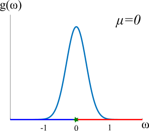
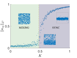
a  b
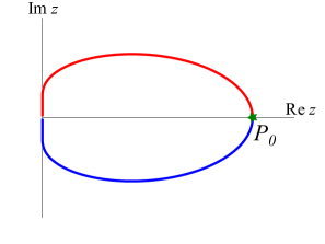
c  d

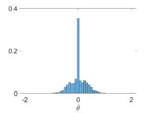
Figure 1: a) A graph of an even unimodal probability density function $g$. b) The corresponding critical curve $\mathcal{C}$ intersects postive real semiaxis at a unique point $P_{0}$. The preimage of $P_{0}$ under $G$ is indicated by the green star in (a). $P_{0}$ corresponds to the PF bifurcation of mixing resulting in a PLS, which is then gradually transformed into synchronous state (see (c)). d) The velocity distribution within the PLS near PF bifurcation is determined by the eigenfunction (3.4). The normalized histogram of the velocities within the PLS.

3.1 Unimodal $g$

We are now prepared to discuss the bifurcations in the KM. We start with the case of an even unimodal $g$ (see Fig. 1a). Although the bifurcation of mixing leading to the transition to synchrony for such $g$ is well understood (cf. [31, 30, 3, 11]), we use it as an example to explain the Penrose’s method. Below, we will apply this method to study bifurcations in a families of bi- and tri- modal distributions (Figs. 2, 5).

Using the symmetry of $g$, from (3.3) we see that $\mathcal{C}$ is symmetric about the $x$–axis. It intersects the positive real semiaxis at a unique point $P_{0}=(x_{0},0),x_{0}>0$. Further, note that $G^{-1}(x_{0})=0$ (Figure 2a, b). From the $x$–equation in (3.3) we find $x_{0}=\pi g(0)$. By the Argument Principle, the number of roots of (3.1) in $\mathbb{H}^{+}$ is equal to the winding number of $\mathcal{C}$ about $K^{-1}$ [26]. Since for $K<K_{c}:=(\pi g(0))^{-1}$, $K^{-1}$ lies outside $\mathcal{C}$ (Fig. 1b), and the winding number is $0$. We conclude that for $K<K_{c}$, $\bm{T}$ has no eigenvalues with positive real parts. Thus, for $K<K_{c}$, mixing is linearly stable. In fact, it is asymptotically stable [7, Theorem 4.1]. For $K>K_{c}$, on the other hand, the winding number is $1$. As $K\to K_{c}+0$, $\lambda\to 0+$, and at $K=K_{c}$, mixing undergoes a PF bifurcation. Using (2.17) and (2.20), we compute the eigenfunction corresponding to $\lambda=0$:

$$\upsilon_{0}(\omega,x)=\pi g(0)\delta_{0}(\omega)-{i\mkern 1.0mu}\mathcal{P}_{0}[g](\omega).$$ (3.4)

Each term on the right–hand side of (3.4) has a singularity at $0$. The second term also has a regular component. This determines the structure of the PLS bifurcating from the mixing state (Fig. 1c). The delta function on the right–hand side of (3.4) implies that the coherent cluster within the PLS is stationary. The regular component of ${i\mkern 1.0mu}\mathcal{P}_{0}[g]$ yields the velocity distribution within the incoherent group. The combination of these two terms yields the velocity distribution within the PLS.

3.2 Bimodal $g$

Next, we turn to the description of a bifurcation scenario connecting mixing to chimeras through $2$–clusters. To this end, we continuously deform the unimodal distribution $g$ into a bimodal distribution, preserving even symmetry as shown in Fig. 2a,b. In our numerical experiments, we use the following family of probability distribution functions:

$$g^{\mu}_{\sigma_{1},\sigma_{2}}(x)=\frac{1}{2\sqrt{2\pi}}\left\{\frac{e^{{-(x+\mu)^{2}\over 2\sigma_{1}^{2}}}}{\sigma_{1}}+\frac{e^{{-(x-\mu)^{2}\over 2\sigma_{2}^{2}}}}{\sigma_{2}}\right\}$$ (3.5)

When $\sigma_{1}=\sigma_{2}=:\sigma$, we collapse indices into one $g^{\mu}_{\sigma}:=g^{\mu}_{\sigma,\sigma}$. First, we keep $\sigma_{1}=\sigma_{2}=:\sigma$ and increase $\mu$ from zero. We want to understand how the critical curve changes as $\mu$ is varied. The key events in the metamorphosis of $\mathcal{C}$ are shown Fig. 2d, e. For small $\mu>0$, $\mathcal{C}_{\mu}$ is diffeomorphic to $\mathcal{C}_{0}$ in a neighborhood of $P_{0}$, the point the intersection of $\mathcal{C}_{0}$ with the real axis. At a critical value $\mu^{\ast}>0$, $\mathcal{C}_{\mu^{\ast}}$ develops a cusp at $P_{\mu^{\ast}}$ (see Fig. 2d). To identify the condition for the cusp, we look for the value of $\mu$, at which the condition of the Inverse Function Theorem fails for $G$. By (3.3) this occurs when $\left.dy/dt\right|_{t=0}=0$, i.e.,

$$J[g^{\mu^{\ast}}_{\sigma}]:=\int_{0}^{\infty}\frac{(g^{\mu^{\ast}}_{\sigma})^{\prime}(s)}{s}ds=0$$ (3.6)

(see Fig. 3a).

For $\mu>\mu^{\ast}$ there is a point on the real axis $P_{\mu}$, which has two preimages under $G$: $\pm{i\mkern 1.0mu}\nu$ (Fig. 2b, e). Thus, for $\mu>\mu^{\ast}$ mixing loses stability through the AH bifurcation and not through the PF bifurcation. At the AH bifurcation, $\bm{T}$ has a pair of complex conjugate eigenvalues $\pm{i\mkern 1.0mu}\nu$. The corresponding eigenfunctions are given by (2.17), (2.19)

$$v_{\pm{i\mkern 1.0mu}\nu+0}=\pi g^{\mu}_{\sigma}(\pm\nu)\delta_{\pm\nu}-{i\mkern 1.0mu}\mathcal{P}_{\pm\nu}[g_{\sigma}^{\mu}].$$ (3.7)

The first term on the right-hand side of $v_{{i\mkern 1.0mu}\nu+0}$ (cf. (3.7)) is localized at $\omega=\nu$. The second term is singular at $\nu$ too, but also has a regular component. The combination of of $v_{{i\mkern 1.0mu}\nu+0}$ and $v_{-{i\mkern 1.0mu}\nu+0}$ results in splitting the population into two groups of approximately equal size rotating with the velocities centered around $\pm\nu$. Thus, for $\mu>\mu^{\ast}$ mixing bifurcates into a $2$–cluster state. At $\mu=\mu^{\ast}$, where the regions of the PF and AH bifurcations meet, we have a codimension–$2$ bifurcation, whose unfolding contains the transitions to synchronization, $2$–clusters, and to chimeras, as we are going to see next.

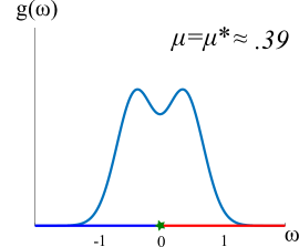
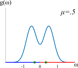
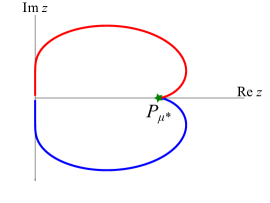
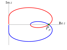
a b c
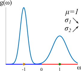
d e f

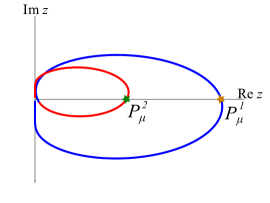
Figure 2: a-c) Continuous deformation of the unimodal symmetric density $g$ into a bimodal asymmetric one (c) and the plots of the corresponding critical curves (d-f). At the critical value $\mu=\mu^{\ast}$, $\mathcal{C}_{\mu^{\ast}}$ develops a cusp (d). This corresponds to the codimension–$2$ bifurcation of mixing. The preimages of points of the intersection of the critical curve with the real axis $P_{\mu}$ and $P_{\mu}^{1,2}$ in (d-f) are indicated by stars in the corresponding plots in (a-c).

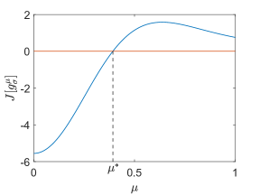
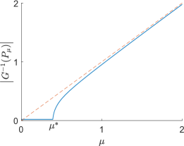
a b c

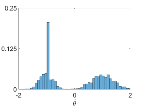
Figure 3: a) The plot of $J[g_{\sigma}^{\mu}]$ vs $\mu$ (cf. (3.6)). The zero of $J[g^{\mu}_{\sigma}]$ determines the critical value $\mu^{\ast}$. b) The plot of the absolute value of the two preimages $G^{-1}(P_{\mu})$. Note that for $\mu>\mu^{\ast}$ outside a small neighborhood of $\mu^{\ast}$, $\left|G^{-1}(P_{\mu})\right|\approx\mu,$ i.e., the two preimages of $P_{\mu}$ lie near the peaks of the density $g$. c) The histogram of the velocity distribution within a chimera is fully determined by the singular distribution $v_{{i\mkern 1.0mu}t_{\mu}+0}$ (cf. (3.8)).

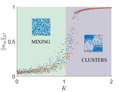
a b

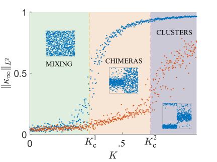
Figure 4: The bifurcation diagrams corresponding to the symmetric and asymmetric bimodal distributions for all–to–all (a and b, respectively). Colored dots indicate the value of the order parameter computed for each cluster separately for different values of $K$ and different realizations of $\omega_{i}$’s. Dots of different colors represent different clusters. In (a), the loss of stability of mixing results in the creation of a $2$–cluster state. In (b), a chimera is born at the loss of stability of mixing at $K_{c}^{1}$. It bifurcates into a moving $2$–cluster at $K_{c}^{2}$. Here, $\kappa_{\infty}(x)$ stands for the asymptotic value of the local order parameter $\kappa(t,x)$ (cf. (2.3)). Note that the bifurcations at $K_{c}^{1}$ and $K_{c}^{2}$ affect clusters practically separately.

We now fix $\mu>\mu^{\ast}$ and break the even symmetry of $g^{\mu}_{\sigma}$ by decreasing $\sigma_{1}$ and increasing $\sigma_{2}$ (see Fig. 2c). This affects the critical curve $\mathcal{C}_{\mu,\sigma_{1},\sigma_{2}}$ in the following way. The point of double intersection $P_{\mu}$ splits into two points of intersection with the real axis: $P_{\mu}^{1}=(x_{\mu}^{1},0)$ and $P_{\mu}^{2}=(x_{\mu}^{2},0)$ with $0<x_{\mu}^{2}<x_{\mu}^{1}$ (see Fig. 2f). Note that the preimages of these points under $G$ are still very close to the maxima of $g^{\mu}_{\sigma_{1},\sigma_{2}}$ (see Fig. 2c and Fig. 3b). In particular, the preimage of $P_{\mu}^{1}$ is approximately $-{i\mkern 1.0mu}\mu$, the center of the more localized peak of $g^{\mu}_{\sigma_{1},\sigma_{2}}$ . This implies that mixing loses stability at $K_{c}^{1}\approx(\pi g^{\mu}_{\sigma_{1},\sigma_{2}}(-\mu))^{-1}$. The bifurcating eigenvalue $\lambda={i\mkern 1.0mu}\nu_{1}(\nu_{1}\approx-\mu)$ and the corresponding eigenfunction

$$v_{{i\mkern 1.0mu}\nu_{1}+0}=\pi g^{\mu}_{\sigma_{1},\sigma_{2}}(\nu_{1})\delta_{\nu_{1}}-{i\mkern 1.0mu}\mathcal{P}_{\nu_{1}}[g^{\mu}_{\sigma_{1},\sigma_{2}}].$$ (3.8)

Note that the first term on the right hand side of (3.8) is a singular distribution localized at $\nu_{1}$. The second term has a singularity at $\nu_{1}$, but its regular part has some ’weight’ near $\nu_{2}\approx\mu$. These features translate into the velocity distribution within a chimera: there is a tightly localized peak around $-\mu$ (the coherent group) and a broader peak near $\mu$ (the incoherent group) (Fig. 3c).

From the Penrose diagram in Fig. 2f we can read off the region of existence of chimeras. Recall that $(x_{\mu}^{1,2},0)$ are the points of intersection of $C_{\mu}$ with the real axis (see Fig. 2f). For $K>K^{2}_{c}$, the winding number of $\mathcal{C}_{\mu}$ about $K^{-1}$ is $2$. The second unstable mode is given by

$$v_{{i\mkern 1.0mu}\nu_{2}+0}=\pi g^{\mu}_{\sigma_{1},\sigma_{2}}(\nu_{2})\delta_{\nu_{2}}-{i\mkern 1.0mu}\mathcal{P}_{\nu_{2}}[g^{\mu}_{\sigma_{1},\sigma_{2}}].$$ (3.9)

Recall that $\nu_{2}\approx\mu$. The first term on the right hand side of (3.9) indicates the formation of a coherent cluster moving with velocity approximately equal to $\mu$. Thus, chimera state is transformed into a pair of clusters moving with the speed $\mu$ in opposite directions. We conclude that the chimera state is born at $K^{1}_{c}\approx\left(\pi g^{\mu}_{\sigma_{1},\sigma_{2}}(-\mu)\right)^{-1}$, when mixing loses stability. This corresponds to the first point of intersection of the critical curve with the real axis $P^{1}_{\mu}$ (Fig. 2f). The chimera state dissappears at $K^{2}_{c}\approx\left(\pi g^{\mu}_{\sigma_{1},\sigma_{2}}(\mu)\right)^{-1}$, when the second unstable mode is created. This corresponds to the second intersection point $P^{2}_{\mu}$ (Fig. 2f). The existence region $(K_{c}^{1},K_{c}^{2})$, predicted by the Penrose diagram, agrees extremely well with numerical simulations (Fig. 4b). Moreover, the bifurcations at $K_{c}^{1}$ and $K_{c}^{2}$ affect the coherent and incoherent clusters practically separately. This provides a general mechanism for formation of chimera states. Under more restrictive assumptions a related mechanism of creating chimeras by controlling fluctuations in separate clusters for the KM with inertia was presented in [19].

There is an important distinction between the primary and secondary bifurcations corresponding to points $P_{\mu}^{1}$ and $P_{\mu}^{2}$ in the diagram shown in Figure 2f. The former signals the appearance of the postive eigenvalue in the spectrum of $\bm{T}$, the operator linearized about mixing. This corresponds to the PF bifurcation of mixing at $K=K_{c}^{1}$ (Fig. 4b). The meaning of $P_{\mu}^{2}$ is different. It corresponds to the emergence of the second positive eigenvalue of $\bm{T}$ at $K=K_{c}^{2}$. Apparently, the linearization about mixing is still relevant for values of $K$ near $K_{c}^{2}$, as the two unstable modes of $\bm{T}$ capture the transformations in the system dynamics near $K_{c}^{2}$, and $(K_{c}^{1},K_{c}^{2})$ provides a good estimate of the region of existence of chimera states (Fig. 4b). The secondary bifurcation at $K_{c}^{2}$ may not be a bifurcation in the strict sense of the word, but it is useful for interpretting the spatial patterns in the KM (Fig. 4b), as it marks the end of the region for chimeras.

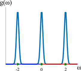
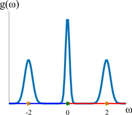
a b c

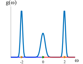
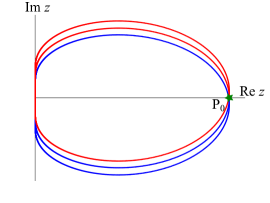
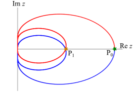
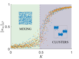
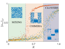
d e f
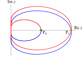
g h i

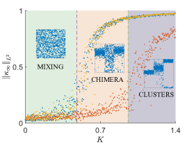
Figure 5: a-c) A family of trimodal probability distributions (3.10). d-f) The corresponding critical curves. Under the deformation of the density functions, the point of triple intersection in d splits into a point of simple intersection and a point of double intersection e and f. Each point of simple intersection corresponds to a PF bifurcation producing a pattern with a stationary cluster, whereas a point of double intersection corresponds an AH bifurcation resulting in patterns with a pair of moving clusters. The bifurcation scenarios predicted by the diagrams in d-f are shown in g-i. They are explained in the text.

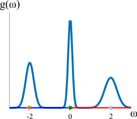
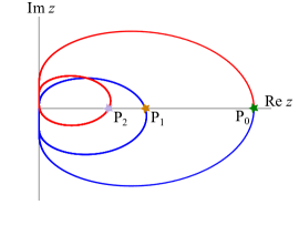
a b c

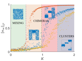
Figure 6: Symmetry breaking in the trimodal distribution shown in Figure 5b results in splitting of the point of the double intersection into two simple intersection points. Thus, the Penrose diagram predicts a PF bifurcation and two secondary bifurcations. The former produces a chimera with the stationary coherent cluster in the middle (c, beige), the first secondary bifurcation results in a chimera with two coherent clusters (a stationary cluster in the middle and a traveling one on the left) (c, pink), and the last secondary bifurcation produces a three-cluster state with the stationary middle cluster and two clusters rotating in opposite directions (c, purple).

3.3 Trimodal $g$

To give a more complete picture of possible bifurcation scenarios in the KM with multimodal distributions of the intrinsic frequencies, we discuss bifurcations in the KM with trimodal family of distributions. In the numerical experiments used in this section, we take the probability distribution functions of the following form:

$$g^{\mu}_{\sigma_{1},\sigma_{2},\sigma_{3}}(x)=\frac{1}{3\sqrt{2\pi}}\left\{\frac{e^{{-(x+\mu)^{2}\over 2\sigma_{1}^{2}}}}{\sigma_{1}}+\frac{e^{{-x^{2}\over 2\sigma_{2}^{2}}}}{\sigma_{2}}+\frac{e^{{-(x-\mu)^{2}\over 2\sigma_{3}^{2}}}}{\sigma_{3}}\right\}.$$ (3.10)

To study bifurcations in the model with trimodal frequency distribution we employ the same strategy as above. We first locate the highest codimension master bifurcation of mixing, whose unfolding contains all principal bifurcation scenarios. To this end, we fix $\mu>0$ and choose $\sigma_{1},\sigma_{2},$ $\sigma_{3}$ so that the critical curve $\mathcal{C}$ has a point of triple intersection with the real axis $P_{0}$ (see Fig. 5d). In our numerical simulations, we used $\mu=2$ and $\sigma_{2}=0.2$, and $\sigma_{1}=\sigma_{3}\approx 0.1976$, i.e., all peaks are practically the same (see Fig. 5a). The intersection point $P_{0}$ has three preimages under $G$: $G^{-1}(P_{0})\approx\{\pm 2i,0\}$. Thus, the loss of stability of mixing takes place through a PF-AH bifurcation. The diagram in Fig. 5g shows the bifurcation of mixing producing a $3$-cluster state. The middle cluster is stationary as implied by the PF bifurcation and the two outer clusters are moving with opposite velocities as implied by the AH bifurcation.

Next, we deform the distribution in Figure 5a reserving even symmetry in two different ways. First, we increase $\sigma_{1}$ and $\sigma_{3}$ keeping them equal (see Figure 5b). Under this deformation, the triple intersection point splits into a simple intersection point $P_{0}$ and a point of double intersection $P_{1}$ (see Figure 5e). This results in a PF bifurcation followed by the AH bifurcation. The former produces a chimera state with a stationary middle cluster, which is further transformed into a three-cluster state with a stationary cluster in the middle and two rotating clusters on the sides (see Figure 5h). An alternative scenario is shown in the last column of Figure 5. This time the AH bifurcation comes first and, therefore, we get a chimera state with two traveling coherent clusters on the sides. After the PF bifurcation, we arrive at the same three-cluster pattern as above (see Figure 5i). Finally, we break the even symmetry of $g$ by increasing $\sigma_{3}$. Without symmetry constraints, the point of triple intersection splits into three simple points $P_{0},P_{1},$ and $P_{2}$ (see Figure 6b). Thus, we have a sequence of a PF bifurcation and two secondary bifurcations making clusters coherent and stationary one by one (see Figure 6c). The eventual state is a stationary three-cluster state.

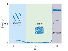
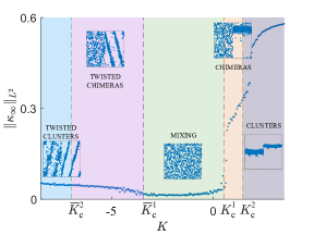
a b c

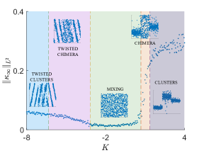
Figure 7: Bifurcation diagrams for the KM with nonlocal nearest-neighbor coupling and uni-, bi-, and tri- modal frequency distributions shown in plots a, b, and c respectively. In all simulations the nearest neighbor coupling range is $r=0.3$. In (a) the PF bifurcation leading to synchronization for positive $K$ has a counterpart for $K$ negative. The latter results in the emergence of stationary twisted states. The same principle applies to the bifurcation diagrams in b and c: bifurcations for positive $K$ have mirror images for negative $K$ with coherent structures superimposed on twisted states. For instance, diagram b features twisted chimera and clusters of traveling twisted states generated from the bimodal distribution in Fig. 2c. Using the trimodal distribution from Fig. 5c, we obtain the 3-clusters shown in c, two outer clusters contain traveling twisted states and the middle one presents a stationary twisted states. The cluster type (stationary vs traveling) is determined by the underlying bifurcation. The AH bifurcation results in a pair of traveling coherent structures, whereas PF bifurcation produces a stationary one (see text for details). Oscillators in the snapshots are reordered in order to easily distinguish the separate clusters.

4 Adding connectivity

Network connectivity can have a profound effect on the spatial organization of chimera states. In the previous section, we discussed bifurcation scenarios in the KM with all–to–all coupling, i.e., for $W\equiv 1$. In this case, the largest eigenvalue of $\bm{W}$ is $1$ and the corresponding eigenfunction is $w\equiv 1$. There are no negative eigenvalues. This has the following implications. Mixing is stable for $K\in(-\infty,K_{c})$ and patterns emerging at the bifurcation at $K_{c}$ are spatially homogeneous, because $v_{\lambda}(\omega,x)$ in (2.17) does not depend on $x$. In general, $\bm{W}$ may have eigenvalues of both signs [6]. In this case, along with the bifurcations at positive $K_{c}^{1}$ and $K_{c}^{2}$ identified above there are negative counterparts at $\bar{K}_{c}^{2}<\bar{K}_{c}^{1}<0$. The eigenfunctions corresponding to negative eigenvalues of $\bm{W}$ are no longer constant and they endow the bifurcating patterns (clusters and chimeras) with a nontrivial spatial organization. We refer an interested reader to [10, 8, 6] for more details on the KM with nonconstant $W$.

Suppose $\bm{W}$ has eigenvalues of both signs and denote the largest positive and smallest negative eigenvalues of $\bm{W}$ by $\mu^{+}$ and $\mu^{-}$ respectively. Then the region of stability of mixing is bounded $K\in(K_{c}^{-},K_{c}^{+}),$ with $K_{c}^{-}<0<K_{c}^{+}$. Furthermore, one of the eigenfunctions corresponding to $\mu^{-}$ or $\mu^{+}$ is not constant. Thus, the patterns emerging from one of the bifurcations will have spatial structure.

To illustrate these effects, we consider the KM with nonlocal nearest neighbor coupling. To this end, let $W(x,y)=V(x-y)$, which is defined by

$$V(x)=\mathbf{1}_{(-r,r)}(x),\quad\mbox{on}\;(-1/2,1/2)$$

and extended to $\mathbb{R}$ by periodicity. Here, $\mathbf{1}$ stands for the indicator function, and $r\in(0,1/2)$ is a fixed parameter. Then

$$\bm{W}[f](x)=\int_{0}^{1}V(x-y)f(y)dy.$$

The eigenvalues of $\bm{W}$ can be computed explicitly

$$\mu_{k}=\int_{0}^{1}V(x)e^{\pm 2\pi{i\mkern 1.0mu}kx}dx=\int_{0}^{1}V(x)\cos\left(2\pi kx\right)dx,\quad k=0,1,2,\dots.$$

The corresponding eigenfunctions are $w_{k}=e^{\pm 2\pi{i\mkern 1.0mu}kx}$. The largest positive eigenvalue is $\mu^{+}=2r$ (cf. [6, Lemma 5.3]). By $k^{\ast}>0$ denote the value of $k$ corresponding to the smallest negative eigenvalue of $\bm{W}$, $\mu_{k^{\ast}}$. The corresponding eigenfunctions are $e^{2\pi{i\mkern 1.0mu}k^{\ast}x}$ and $e^{-2\pi{i\mkern 1.0mu}kx}$.

To explain the implications of the presence of the eigenvalues of both signs in the spectrum of $\bm{W}$, we first turn to the unimodal distribution. If $g$ is even and unimodal then the region of stability of mixing is a bounded interval $(K_{c}^{-},K_{c}^{+})$ with $K_{c}^{-}=\pi(g(0)\mu^{-})^{-1}$ and $K_{c}^{+}=\pi(g(0)\mu^{+})^{-1}$ [6]. At $K_{c}^{+}$ we observe a familiar scenario of transition to synchronization (Figure 7). At $K_{c}^{-}$ the situation is different. The center subspace of the linearized problem in the Fourier space is spanned by

$$v_{\mu^{-}}^{(1)}=\Upsilon_{0}(\omega)e^{2\pi{i\mkern 1.0mu}k^{\ast}x}\quad\mbox{and}\quad v_{\mu^{-}}^{(2)}=\Upsilon_{0}(\omega)e^{-2\pi{i\mkern 1.0mu}k^{\ast}x}.$$

In the solution space, we therefore expect that

$$f(t,\theta,\omega,x)\sim\operatorname{Re}\left(c_{1}+c_{2}\Upsilon_{0}(\omega)e^{2\pi{i\mkern 1.0mu}(\pm k^{\ast}x-\theta)}\right),\quad c_{1},c_{2}\in\mathbb{C}.$$

For the PLS emerging at the bifurcation, we see that the structure encoded in $\Upsilon(\omega)$ is now superimposed onto a $k^{\ast}$–twisted state (Fig. 7a). The same principle applies to all other bifurcation scenarios, which we discussed for bi- and trimodal distributions in the previous section. Specifically, whenever a transition to coherence occurs whether in a cluster or in the entire population, the nascent coherent structure is superimposed onto a twisted state.

Plots b and c of Figure 7 present bifurcation diagrams for families of bimodal and trimodal distributions. The bifurcations for positive $K$ analyzed in the previous sections have counterparts for negative $K$. The latter feature (traveling) twisted states every time the transition to coherence takes place. The velocity of the twisted states is determined by the corresponding eigenvalues of $\bm{T}$ as before. The appearance of twisted states in this model is a consequence of anisotropic coupling. Whenever $W(x,y)=V(x-y)$ for some function $V$ on a unit circle, the eigenfunctions of $\bm{W}$ are exponential functions $e^{2\pi{i\mkern 1.0mu}kx}$. By varying $W$, one can achieve a variety of spatial patterns born when mixing loses stability.

5 Discussion

In this paper, we studied bifurcations in the KM with multimodal frequency distributions. We showed that the loss of stability of mixing in this model leads to different patterns including stationary and traveling clusters and chimera states. In structured networks these patterns acquire additional spatial organization. In particular, bifurcations of mixing in the KM with nonlocal nearest-neighbor coupling give rise to twisted chimera states with regions of coherent behavior organized as stationary or traveling twisted states. The combination of the linear stability analysis, Penrose diagrams, and the spectral properties of the graph limit provide information about all essential features of the complex spatiotemporal patterns found in the KM after mixing loses statbility. In particular, we were able to identify velocity distribution within chimera states as well the region of their existence.

The type of the bifurcation determines the dynamical properties of the nascent patterns. The PF bifurcation results in stationary clusters, whereas an AH bifurcation produces traveling clusters. Furthermore, we described a codimension-2 and a codimension-3 PF-AH bifurcation, whose unfolding contain transitions to stationary and traveling clusters and chimera states in the KM with bi- and trimodal frequency distributions (Figs. 4, 5, 6).

To locate the bifurcations of mixing and subsequent (secondary) bifurcations leading to clusters or chimera states we used Penrose’s diagrams, which reduce the problem to the analysis of geometric and topological properties of a closed critical curve. Once the bifurcations are found, the emerging patterns are determined by the unstable modes, i.e., the eigenfunctions of the linearized operator corresponding to the eigenvalues with zero real parts. In particular, the unstable modes determine the velocity distributions within PLS and chimera states.

Our analysis of primary bifurcations of mixing relies on rigorous mathematical theory available for the KM [6, 7, 5, 11]. Our treatment of the secondary bifurcations should be considered as experimental. It predicts very well the emergence of chimeras, their statistical properties, and the domain of existence, but the mathematical basis of these findings should be investigated further. Nonetheless, our results show that the combination of the linear stability analysis and the geometric method of Penrose provide a simple and effective way for understanding pattern formation in the KM with multimodal frequency distribution. We believe that the bifurcation scenarios described in this paper are relevant to other interacting particle systems. In particular, the same method works well for the KM with inertia [19]. It reveals similar and more sophisticated patterns for the model with inertia. These results will be presented elsewhere.

Since their discovery chimeras have appealed to a broad community of mathematicians and physicists as a stark example of highly heterogeneous structures produced by homogeneous systems. An inquisitive reader might note that in contrast to the model in [2], where all $\omega_{i}$’s are the same, in our case $\omega_{i}$’s are different, and so the system is not homogeneous. In response, we note if (1.1) is rewritten as

$$\begin{split}\dot{\theta}_{i}&=\omega_{i}+\frac{2K}{n}\sum_{j=1}^{n}a^{n}_{ij}\sin(\theta_{j}-\theta_{i}+\alpha),\\ \dot{\omega}_{i}&=0,\quad i\in[n],\end{split}$$ (5.1)

then the right-hand sides in all equations have the same form, and heterogeneity enters only through the initial conditions. In this respect, our setting is not different from that in [2].

Acknowledgements. This work was supported in part by NSF grant DMS 2009233 (to GSM). Numerical simulations were completed using the high performance computing cluster (ELSA) at the School of Science, The College of New Jersey. Funding of ELSA is provided in part by NSF OAC-1828163. MSM was additionally supported by a Support of Scholarly Activities Grant at The College of New Jersey.

References

- [1] Daniel M. Abrams, Rennie Mirollo, Steven H. Strogatz, and Daniel A. Wiley, Solvable model for chimera states of coupled oscillators, Phys. Rev. Lett. 101 (2008), 084103.
- [2] Daniel M. Abrams and Steven H. Strogatz, Chimera states in a ring of nonlocally coupled oscillators, Internat. J. Bifur. Chaos Appl. Sci. Engrg. 16 (2006), no. 1, 21–37.
- [3] Hayato Chiba, A proof of the Kuramoto conjecture for a bifurcation structure of the infinite-dimensional Kuramoto model, Ergodic Theory Dynam. Systems 35 (2015), no. 3, 762–834.
- [4] , A spectral theory of linear operators on rigged Hilbert spaces under analyticity conditions, Adv. Math. 273 (2015), 324–379.
- [5] Hayato Chiba, A Hopf bifurcation in the Kuramoto-Daido model, arXiv 1610.02834, 2016.
- [6] Hayato Chiba and Georgi S. Medvedev, The mean field analysis of the Kuramoto model on graphs I. The mean field equation and transition point formulas, Discrete Contin. Dyn. Syst. 39 (2019), no. 1, 131–155.
- [7] , The mean field analysis of the Kuramoto model on graphs II. Asymptotic stability of the incoherent state, center manifold reduction, and bifurcations, Discrete Contin. Dyn. Syst. 39 (2019), no. 7, 3897–3921.
- [8] Hayato Chiba, Georgi S. Medvedev, and Matthew S. Mizuhara, Bifurcations in the Kuramoto model on graphs, Chaos 28 (2018), no. 7, 073109, 10.
- [9] Hayato Chiba, Georgi S. Medvedev, and Matthew S. Mizuhara, Instability of mixing in the Kuramoto model: From bifurcations to patterns, arXiv e-prints (2020), arXiv:2009.00103.
- [10] Hayato Chiba, Georgi S. Medvedev, and Matthew S. Mizuhara, in preparation.
- [11] Helge Dietert, Stability and bifurcation for the Kuramoto model, J. Math. Pures Appl. (9) 105 (2016), no. 4, 451–489. MR 3471147
- [12] Dawid Dudkowski, Yuri Maistrenko, and Tomasz Kapitaniak, Occurrence and stability of chimera states in coupled externally excited oscillators, Chaos 26 (2016), no. 11, 116306, 9.
- [13] Dmitry Kaliuzhnyi-Verbovetskyi and Georgi S. Medvedev, The mean field equation for the kuramoto model on graph sequences with non-lipschitz limit, SIAM Journal on Mathematical Analysis 50 (2018), no. 3, 2441–2465.
- [14] Y. Kuramoto and D. Battogtokh, Coexistence of coherence and incoherence in nonlocally coupled phase oscillators, Nonlinear Phenomena in Complex Systems 5 (2002), 380–385.
- [15] Carlo R. Laing, The dynamics of chimera states in heterogeneous Kuramoto networks, Phys. D 238 (2009), no. 16, 1569–1588.
- [16] C. Lancellotti, On the Vlasov limit for systems of nonlinearly coupled oscillators without noise, Transport Theory Statist. Phys. 34 (2005), no. 7, 523–535. MR 2265477 (2007f:82098)
- [17] L. Lovász, Large networks and graph limits, AMS, Providence, RI, 2012.
- [18] Georgi S. Medvedev, The continuum limit of the Kuramoto model on sparse random graphs, Commun. Math. Sci. 17 (2019), no. 4, 883–898.
- [19] Georgi S. Medvedev and Mathew S. Mizuhara, Stability of Clusters in the Second-Order Kuramoto Model on Random Graphs, J. Stat. Phys. 182 (2021), no. 2, 30.
- [20] Simbarashe Nkomo, Mark R. Tinsley, and Kenneth Showalter, Chimera and chimera-like states in populations of nonlocally coupled homogeneous and heterogeneous chemical oscillators, Chaos 26 (2016), no. 9, 094826, 10.
- [21] O. E. Omel’chenko, The mathematics behind chimera states, Nonlinearity 31 (2018), no. 5, 121–164.
- [22] O.E. Omelchenko, Coherence-incoherence patterns in a ring of non-locally coupled phase oscillators, Nonlinearity 26 (2013), no. 9, 2469.
- [23] Oleh E. Omel’chenko, Yuri L. Maistrenko, and Peter A. Tass, Chimera states: The natural link between coherence and incoherence, Phys. Rev. Lett. 100 (2008), 044105.
- [24] Edward Ott and Thomas M. Antonsen, Low dimensional behavior of large systems of globally coupled oscillators, Chaos 18 (2008), no. 3, 037113, 6.
- [25] Mark J. Panaggio and Daniel M. Abrams, Chimera states: coexistence of coherence and incoherence in networks of coupled oscillators, Nonlinearity 28 (2015), no. 3, R67–R87.
- [26] Oliver Penrose, Electrostatic instabilities of a uniform non‐maxwellian plasma, The Physics of Fluids 3 (1960), no. 2, 258–265.
- [27] Francisco A. Rodrigues, Thomas K. DM. Peron, Peng Ji, and Jürgen Kurths, The Kuramoto model in complex networks, Physics Reports 610 (2016), 1 – 98, The Kuramoto model in complex networks.
- [28] Lennart Schmidt, Konrad Schönleber, Katharina Krischer, and Vladimir García-Morales, Coexistence of synchrony and incoherence in oscillatory media under nonlinear global coupling, Chaos 24 (2014), no. 1, 013102, 7.
- [29] Barry Simon, Basic Complex Analysis, A Comprehensive Course in Analysis, Part 2A, American Mathematical Society, Providence, RI, 2015.
- [30] Steven H. Strogatz, From Kuramoto to Crawford: exploring the onset of synchronization in populations of coupled oscillators, Phys. D 143 (2000), no. 1-4, 1–20, Bifurcations, patterns and symmetry.
- [31] Steven H. Strogatz and Renato E. Mirollo, Stability of incoherence in a population of coupled oscillators, J. Statist. Phys. 63 (1991), no. 3-4, 613–635.