Decision Making with Differential Privacy under a Fairness Lens

Abstract

Agencies, such as the U.S. Census Bureau, release data sets and statistics about groups of individuals that are used as input to a number of critical decision processes. To conform with privacy and confidentiality requirements, these agencies are often required to release privacy-preserving versions of the data. This paper studies the release of differentially private data sets and analyzes their impact on some critical resource allocation tasks under a fairness perspective. The paper shows that, when the decisions take as input differentially private data, the noise added to achieve privacy disproportionately impacts some groups over others. The paper analyzes the reasons for these disproportionate impacts and proposes guidelines to mitigate these effects. The proposed approaches are evaluated on critical decision problems that use differentially private census data.

1 Introduction

Many agencies or companies release statistics about groups of individuals that are often used as inputs to critical decision processes. The U.S. Census Bureau, for example, releases data that is then used to allocate funds and distribute critical resources to states and jurisdictions. These decision processes may determine whether a jurisdiction must provide language assistance during elections, establish distribution plans of COVID-19 vaccines for states and jurisdictions [20], and allocate funds to school districts [16, 11]. The resulting decisions may have significant societal, economic, and medical impacts for participating individuals.

In many cases, the released data contain sensitive information whose privacy is strictly regulated. For example, in the U.S., the census data is regulated under Title 13 [1], which requires that no individual be identified from any data released by the Census Bureau. In Europe, data release is regulated according to the General Data Protection Regulation [12], which addresses the control and transfer of personal data. As a result, such data releases must necessarily rely on privacy-preserving technologies. Differential Privacy (DP) [6] has become the paradigm of choice for protecting data privacy, and its deployments have been growing rapidly in the last decade. These include several data products related to the 2020 release of the US. Census Bureau [2], Apple [22], Google [10], and Uber [14], and LinkedIn [19].

Although DP provides strong privacy guarantees on the released data, it has become apparent recently that differential privacy may induce biases and fairness issues in downstream decision processes, as shown empirically by Pujol et al. [16]. Since at least $675 billion are being allocated based on U.S. census data [16], the use of differential privacy without a proper understanding of these biases and fairness issues may adversely affect the health, well-being, and sense of belonging of many individuals. Indeed, the allotment of federal funds, apportionment of congressional seats, and distribution of vaccines and therapeutics should ideally be fair and unbiased. Similar issues arise in several other areas including, for instance, election, energy, and food policies. The problem is further exacerbated by the recent recognition that commonly adopted differential privacy mechanisms for data release tasks may in fact introduce unexpected biases on their own, independently of a downstream decision process [27].

This paper builds on these empirical observations and provides a step towards a deeper understanding of the fairness issues arising when differentially private data is used as input to several resource allocation problems. One of its main results is to prove that several allotment problems and decision rules with significant societal impact (e.g., the allocation of educational funds, the decision to provide minority language assistance on election ballots, or the distribution of COVID-19 vaccines) exhibit inherent unfairness when applied to a differentially private release of the census data. To counteract this negative results, the paper examines the conditions under which decision making is fair when using differential privacy, and techniques to bound unfairness. The paper also provides a number of mitigation approaches to alleviate biases introduced by differential privacy on such decision making problems. More specifically, the paper makes the following contributions:

1. It formally defines notions of fairness and bounded fairness for decision making subject to privacy requirements.

2. It characterizes decision making problems that are fair or admits bounded fairness. In addition, it investigates the composition of decision rules and how they impact bounded fairness.

3. It proves that several decision problems with high societal impact induce inherent biases when using a differentially private input.

4. It examines the roots of the induced unfairness by analyzing the structure of the decision making problems.

5. It proposes several guidelines to mitigate the negative fairness effects of the decision problems studied.

To the best of the authors’ knowledge, this is the first study that attempt at characterizing the relation between differential privacy and fairness in decision problems.

2 Preliminaries: Differential Privacy

Differential Privacy [6] (DP) is a rigorous privacy notion that characterizes the amount of information of an individual’s data being disclosed in a computation.

Definition 1.

A randomized algorithm $\mathcal{M}:\mathcal{X}\to\mathcal{R}$ with domain $\mathcal{X}$ and range $\mathcal{R}$ satisfies $\epsilon$-differential privacy if for any output $O\subseteq\mathcal{R}$ and data sets $\bm{x},\bm{x}^{\prime}\in\mathcal{X}$ differing by at most one entry (written $\bm{x}\sim\bm{x}^{\prime}$)

$$\Pr[\mathcal{M}(\bm{x})\in O]\leq\exp(\epsilon)\Pr[\mathcal{M}(\bm{x}^{\prime})\in O].$$ (1)

Parameter $\epsilon\!>\!0$ is the privacy loss, with values close to $0$ denoting strong privacy. Intuitively, differential privacy states that any event occur with similar probability regardless of the participation of any individual data to the data set. Differential privacy satisfies several properties including composition, which allows to bound the privacy loss derived by multiple applications of DP algorithms to the same dataset, and immunity to post-processing, which states that the privacy loss of DP outputs is not affected by arbitrary data-independent post-processing [7].

A function $f$ from a data set $\bm{x}\in\mathcal{X}$ to a result set $R\subseteq\mathbb{R}^{n}$ can be made differentially private by injecting random noise onto its output. The amount of noise relies on the notion of global sensitivity $\Delta_{f}=\max_{\bm{x}\sim\bm{x}^{\prime}}\|f(\bm{x})-f(\bm{x}^{\prime})\|_{1}$, which quantifies the effect of changing an individuals’ data to the output of function $f$. The Laplace mechanism [6] that outputs $f(\bm{x})+\bm{\eta}$, where $\bm{\eta}\in\mathbb{R}^{n}$ is drawn from the i.i.d. Laplace distribution with $0$ mean and scale $\nicefrac{{\Delta_{f}}}{{\epsilon}}$ over $n$ dimensions, achieves $\epsilon$-DP.

Differential privacy satisfies several important properties. Notably, composability ensures that a combination of DP mechanisms preserve differential privacy.

Theorem 1 (Sequential Composition).

The composition $(\mathcal{M}_{1}(\bm{x}),\ldots,\mathcal{M}_{k}(\bm{x}))$ of a collection $\{\mathcal{M}_{i}\}_{i=1}^{k}$ of $\epsilon_{i}$-differentially private mechanisms satisfies $(\epsilon=\sum_{i=1}^{k}\epsilon_{i})$-differential privacy.

The parameter $\epsilon$ resulting in the composition of different mechanism is referred to as privacy budget. Stronger composition results exists [15] but are beyond the need of this paper. Post-processing immunity ensures that privacy guarantees are preserved by arbitrary post-processing steps.

Theorem 2 (Post-Processing Immunity).

Let $\mathcal{M}$ be an $\epsilon$-differentially private mechanism and $g$ be an arbitrary mapping from the set of possible output sequences to an arbitrary set. Then, $g\circ\mathcal{M}$ is $\epsilon$-differentially private.

3 Problem Setting and Goals

The paper considers a dataset $\bm{x}\!\in\!\mathcal{X}\subseteq\mathbb{R}^{k}$ of $n$ entities, whose elements $x_{i}=(x_{i1},\ldots,x_{1k})$ describe $k$ measurable quantities of entity $i\!\in\![n]$, such as the number of individuals living in a geographical region $i$ and their English proficiency. The paper considers two classes of problems:

• An allotment problem $P:\mathcal{X}\times[n]\to\mathbb{R}$ is a function that distributes a finite set of resources to some problem entity. $P$ may represent, for instance, the amount of money allotted to a school district.

• A decision rule $P:\mathcal{X}\times[n]\to\{0,1\}$ determines whether some entity qualifies for some benefits. For instance, $P$ may represent if election ballots should be described in a minority language for an electoral district.

The paper assumes that $P$ has bounded range, and uses the shorthand $P_{i}(\bm{x})$ to denote $P(\bm{x},i)$ for entity $i$. The focus of the paper is to study the effects of a DP data-release mechanism $\mathcal{M}$ to the outcomes of problem $P$. Mechanism $\mathcal{M}$ is applied to the dataset $\bm{x}$ to produce a privacy-preserving counterpart $\tilde{\bm{x}}$ and the resulting private outcome $P_{i}(\tilde{\bm{x}})$ is used to make some allocation decisions.

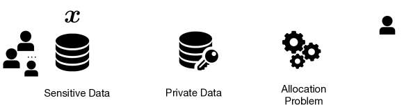
Figure 1: Diagram of the private allocation problem.

Figure 1 provides an illustrative diagram.

Because random noise is added to the original dataset $\bm{x}$, the output $P_{i}(\tilde{\bm{x}})$ incurs some error. The focus of this paper is to characterize and quantify the disparate impact of this error among the problem entities. In particular, the paper focuses on measuring the bias of problem $P_{i}$

$$B_{P}^{i}(\mathcal{M},\bm{x})=\mathbb{E}_{\tilde{\bm{x}}\sim\mathcal{M}(\bm{x})}\left[P_{i}(\tilde{\bm{x}})\right]-P_{i}(\bm{x}),$$ (2)

which characterizes the distance between the expected privacy-preserving allocation and the one based on the ground truth. The paper considers the absolute bias $|B_{P}^{i}|$, in place of the bias $B_{P}^{i}$, when $P$ is a decision rule. The distinction will become clear in the next sections.

The results in the paper assume that $\mathcal{M}$, used to release counts, is the Laplace mechanism with an appropriate finite sensitivity $\Delta$. However, the results are general and apply to any data-release DP mechanism that add unbiased noise.

4 Motivating Problems

This section introduces two Census-motivated problem classes that grant benefits or privileges to groups of people. The problems were first introduced in [16].

Allotment problems

The Title I of the Elementary and Secondary Education Act of 1965 [21] distributes about $6.5 billion through basic grants. The federal allotment is divided among qualifying school districts in proportion to the count $x_{i}$ of children aged 5 to 17 who live in necessitous families in district $i$. The allocation is formalized by

$$P^{F}_{i}(\bm{x})\stackrel{{\scriptstyle\text{def}}}{{=}}\left(\frac{x_{i}\cdot a_{i}}{\sum_{i\in[n]}x_{i}\cdot a_{i}}\right),$$

where $\bm{x}=(x_{i})_{i\in[n]}$ is the vector of all districts counts and $a_{i}$ is a weight factor reflecting students expenditures.

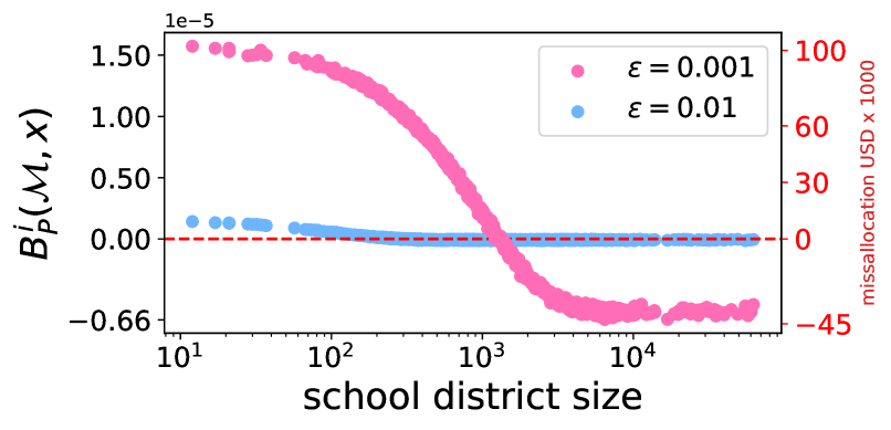
Figure 2: Disproportionate Title 1 funds allotment in NY school districts.

Figure 2 illustrates the expected disparity errors arising when using private data as input to problem $P^{F}$, for various privacy losses $\epsilon$. These errors are expressed in terms of bias (left y-axis) and USD misallocation (right y-axis) across the different New York school districts, ordered by their size. The allotments for small districts are typically overestimated while those for large districts are underestimated. Translated in economic factors, some school districts may receive up to 42,000 dollars less than warranted.

Decision Rules

Minority language voting right benefits are granted to qualifying voting jurisdictions. The problem is formalized as

$$P^{M}_{i}(\bm{x})\!\stackrel{{\scriptstyle\text{def}}}{{=}}\!\left(\frac{x_{i}^{sp}}{x_{i}^{s}}\!>\!0.05\!\lor\!x_{i}^{sp}\!>\!10^{4}\right)\!\land\!\frac{x_{i}^{spe}}{x_{i}^{sp}}\!>\!0.0131.$$

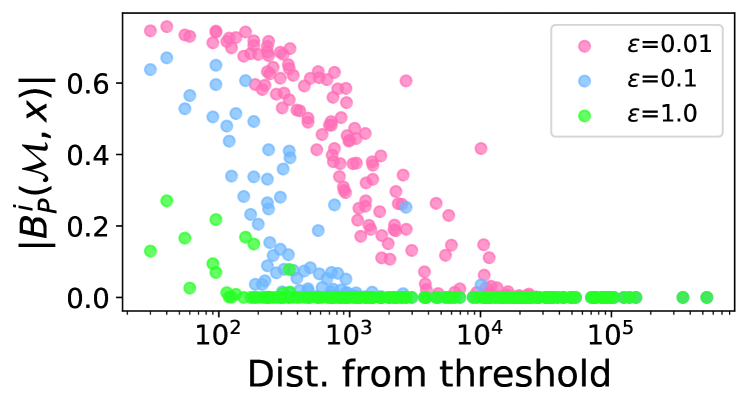
Figure 3: Disproportionate Minority Language Voting Benefits.

For a jurisdiction $i$, $x_{i}^{s}$, $x_{i}^{sp}$, and $x_{i}^{spe}$ denote, respectively, the number of people in $i$ speaking the minority language of interest, those that have also a limited English proficiency, and those that, in addition, have less than a $5^{th}$ grade education. Jurisdiction $i$ must provide language assistance (including voter registration and ballots) iff $P_{i}^{M}(\bm{x})$ is True.

Figure 3 illustrates the decision error (y-axis), corresponding to the absolute bias $|B^{i}_{{P^{M}}}(\mathcal{M},\bm{x})|$, for sorted $x_{i}^{s}$, considering only true positives for the Hispanic language. The figure shows that there are significant disparities in decision errors and that these errors strongly correlate to their distance to the thresholds. These issues were also observed in [16].

5 Fair Allotments and Decision Rules

This section analyzes the fairness impact in allotment problems and decision rules. The adopted fairness concept captures the desire of equalizing the allocation errors among entities, which is of paramount importance given the critical societal and economic impact of the motivating applications.

Definition 2.

A data-release mechanism $\mathcal{M}$ is said fair w.r.t. a problem $P$ if, for all datasets $\bm{x}\in\mathcal{X}$,

$$B_{P}^{i}(\mathcal{M},\bm{x})=B_{P}^{j}(\mathcal{M},\bm{x})\quad\forall i,j\in[n].$$

That is, $P$ does not induce disproportionate errors when taking as input a DP dataset generated by $\mathcal{M}$. The paper also introduces a notion to quantify and bound the mechanism unfairness.

Definition 3.

A mechanism $\mathcal{M}$ is said $\alpha$-fair w.r.t. problem $P$ if, for all datasets $\bm{x}\in\mathcal{X}$ and all $i\in[n]$,

$$\xi_{B}^{i}(P,\mathcal{M},\bm{x})=\max_{j\in[n]}\left|B_{P}^{i}(\mathcal{M},\bm{x})-B_{P}^{j}(\mathcal{M},\bm{x})\right|\leq\alpha,$$

where $\xi_{B}^{i}$ is referred to as the disparity error of entity $i$.

Parameter $\alpha$ is called the fairness bound and captures the fairness violation, with values close to $0$ denoting strong fairness. A fair mechanism is also $0$-fair.

Note that computing the fairness bound $\alpha$ analytically may not be feasible for some problem classes, since it may involve computing the expectation of complex functions $P$. Therefore, in the analytical assessments, the paper recurs to a sampling approach to compute the empirical expectation $\hat{E}[P_{i}(\tilde{\bm{x}})]=\frac{1}{m}\sum_{j\in[m]}P_{i}(\tilde{\bm{x}}^{j})$ in place of the true expectation in Equation (2). Therein, $m$ is a sufficiently large sample size and $\tilde{\bm{x}}^{j}$ is the $j$-th outcome of the application of mechanism $\mathcal{M}$ on data set $\bm{x}$.

5.1 Fair Allotments: Characterization

The first result characterizes a sufficient condition for the allotment problems to achieve finite fairness violations. The presentation uses $\bm{H}P_{i}$ to denote the Hessian of problem $P_{i}$, and $\operatorname{Tr}(\cdot)$ to denote the trace of a matrix. In this context, the Hessian entries are functions receiving a dataset as input. The presentation thus uses $(\bm{H}P_{i})_{j,l}(\bm{x})$ and $\operatorname{Tr}(\bm{H}P_{i})(\bm{x})$ to denote the application of the second partial derivatives of $P_{i}$ and of the Hessian trace function on dataset $\bm{x}$.

Theorem 3.

Let $P$ be an allotment problem that is at least twice differentiable. A data-release mechanism $\mathcal{M}$ is $\alpha$-fair w.r.t. $P$, for some finite $\alpha$, if for all datasets $\bm{x}\in\mathcal{X}$ the entries of the Hessian $\bm{H}P_{i}$ of problem $P_{i}$ are a constant function, that is, if there exists $c^{i}_{jl}\in\mathbb{R}\;(i\in[n],j,l\in[k])$ such that,

$$(\bm{H}P_{i})_{j,l}(\bm{x})=c^{i}_{j,l}\;\;(i\in[n]\;j,l\in[k]).$$ (3)

Proof.

Firstly, notice that the problem bias (Equation 2) can be expressed as

$$B^{i}_{P}(\mathcal{M},\bm{x}) =\mathbb{E}[P_{i}(\tilde{\bm{x}}=\bm{x}+\eta)]-P_{i}(\bm{x})$$ (4a)

$$\approx P_{i}(\bm{x})+\mathbb{E}\left[\eta\nabla P_{i}(\bm{x})\right]+\mathbb{E}\left[\frac{1}{2}\eta^{T}\bm{H}P_{i}(\bm{x})\eta\right]-P_{i}(\bm{x})$$ (4b)

$$=\mathbb{E}\left[\frac{1}{2}\eta^{T}\bm{H}P_{i}(\bm{x})\eta\right]$$ (4c)

$$=\frac{1}{2}\mathbb{E}\left[\sum_{j,k\in[n]}\eta_{j}(\bm{H}P_{i})_{jk}(\bm{x})\eta_{k}\right]$$ (4d)

$$=\frac{1}{2}\mathbb{E}\left[\sum_{j\in[n]}\eta_{j}^{2}(\bm{H}P_{i})_{jj}(\bm{x})\right]$$ (4e)

$$=\frac{1}{2}\sum_{j\in[n]}\mathbb{E}\left[\eta_{j}^{2}\right]\sum_{j\in[n]}\mathbb{E}\left[(\bm{H}P_{i})_{jj}(\bm{x})\right]$$ (4f)

$$=\frac{1}{2}n\mathrm{Var}[\eta]\,\operatorname{Tr}\left(\bm{H}P_{i}\right)(\bm{x}),$$ (4g)

where the approximation (in (4b)) uses a Taylor expansion of the private allotment problem $P_{i}(\bm{x}+\eta)$, where $\eta=\textrm{Lap}(\nicefrac{{\Delta}}{{\epsilon}})$ and the linearity of expectations. Equation (4c) follows from independence of $\eta$ and $\nabla P_{i}(\bm{x})$ and from the assumption of unbiased noise (i.e., $\mathbb{E}[\eta]=0$) and (4e) from independence of the elements of $\eta$ and thus $\mathbb{E}[n_{k}n_{j}]=0$ for $j\neq k$. Finally, (4g) follows from $\mathbb{E}[\eta^{2}]=\mathrm{Var}[\eta]+(\mathbb{E}[\eta])^{2}$ and $\mathbb{E}[\eta]=0$ again, and where $\operatorname{Tr}$ denotes the trace of the Hessian matrix.

The bias $B^{i}_{P}$ can thus be approximated by an expression involving the local curvature of the problem $P_{i}$ and the variance of the noisy input.

Next, by definition of bounded fairness 3

$$\xi_{B}^{i}(P,\mathcal{M},\bm{x})= \max_{j\in[n]}\left|B_{P}^{i}(\mathcal{M},\bm{x})-B_{P}^{j}(\mathcal{M},\bm{x})\right|\leq\alpha$$ (5a)

$$\Leftrightarrow n\mathrm{Var}[\eta]\left|\operatorname{Tr}(\bm{H}P_{i})(\bm{x})-\operatorname{Tr}(\bm{H}P_{j})(\bm{x})\right|\leq\alpha\;\;\forall j\in[n].$$ (5b)

Since, by assumption, there exists constants $c_{k}$ such that $\forall x\in\mathcal{X}$, $\operatorname{Tr}(\bm{H}P_{k})(\bm{x})=\sum_{j,l}c^{k}_{j,l}=c_{k}$ for $k\in[n]$, it follows, that

$$n\mathrm{Var}[\eta]\left|c_{i}-c_{j}\right|<n\mathrm{Var}[\eta]\left(\max_{i\in[n]}c_{i}-\min_{i\in[n]}c_{i}\right)<\infty.$$

∎

The above shed light on the relationship between fairness and the difference in the local curvatures of problem $P$ on any pairs of entities. As long as this local curvature is constant across all entities, then the difference in the bias induced by the noise onto the decision problem of any two entities can be bounded, and so can the (loss of) fairness.

An important corollary of Theorem 3 illustrates which restrictions on the structure of problem $P$ are needed to satisfy fairness.

Corollary 1.

If $P$ is a linear function, then $\mathcal{M}$ is fair w.r.t. $P$.

Proof.

The result follows by noticing that the second derivative of linear function is $0$ for any input. Thus, for any $i\in[n]$, and $\bm{x}\in\mathcal{X},\operatorname{Tr}(\bm{H}P_{i})(\bm{x})=0$. Therefore, from (5b), for every $i\in[n]$,

$$\xi_{B}^{i}(P,\mathcal{M},\bm{x}) =\max_{j\in[n]}\left|\operatorname{Tr}(\bm{H}P_{i})(\bm{x})-\operatorname{Tr}(\bm{H}P_{j})(\bm{x})\right|=0.$$

∎

A more general result is the following.

Corollary 2.

$\mathcal{M}$ is fair w.r.t. $P$ if there exists a constant $c$ such that, for all dataset $\bm{x}$,

$$\operatorname{Tr}(\bm{H}P_{i})(\bm{x})=c\;\;(i\in[n]).$$

The proof is similar, in spirit, to proof of Corollary 1, noting that, in the above, the constant $c$ is equal among all Traces of the Hessian of problems $P_{i}$ $(i\in[n])$.

5.2 Fair Decision Rules: Characterization

The next results bound the fairness violations of a class of indicator functions, called thresholding functions, and discusses the loss of fairness caused by the composition of boolean predicates, two recurrent features in decision rules. The fairness definition adopted uses the concept of absolute bias, in place of bias in Definition 2. Indeed, the absolute bias $|B^{i}_{P}|$ corresponds to the classification error for (binary) decision rules of $P_{i}$, i.e., $\Pr[P_{i}(\tilde{\bm{x}})\neq P_{i}(\bm{x})]$. The results also assume $\mathcal{M}$ to be a non-trivial mechanism, i.e., $|B^{i}_{P}(\mathcal{M},\bm{x})|<0.5\,\forall i\in[n]$. Note that this is a non-restrictive condition, since the focus of data-release mechanisms is to preserve the quality of the original inputs, and the mechanisms considered in this paper (and in the DP-literature, in general) all satisfy this assumption.

Theorem 4.

Consider a decision rule $P_{i}(\bm{x})\!=\!\mathbbm{1}\{x_{i}\!\geq\ \ell\}$ for some real value $\ell$. Then, mechanism $\mathcal{M}$ is $0.5$-fair w.r.t. $P_{i}$.

Proof.

From Definition 3 (using the absolute bias $|B^{i}_{P}(\mathcal{M},\bm{x})|$), and since the absolute bias is always non-negative, it follows that, for every $i\in[n]$:

$$\xi_{B}^{i}(P,\mathcal{M},\bm{x}) =\max_{j\in[n]}\left||B_{P}^{i}(\mathcal{M},\bm{x})|-|B_{P}^{j}(\mathcal{M},\bm{x})|\right|$$ (6a)

$$\leq\max_{j\in[n]}|B_{P}^{j}(\mathcal{M},\bm{x})|-\min_{j\in[n]}|B_{P}^{j}(\mathcal{M},\bm{x})|$$ (6b)

$$\leq\max_{j\in[n]}|B_{P}^{j}(\mathcal{M},\bm{x})|.$$ (6c)

Thus, by definition, mechanism $\mathcal{M}$ is $\max_{j\in[n]}|B^{P}_{j}(\mathcal{M},\bm{x})|$-fair w.r.t. problem $P$. The following shows that the maximum absolute bias $\max_{j\in[n]}|B^{P}_{j}(\mathcal{M},\bm{x})|\leq 0.5$. W.l.o.g. consider an entry $i$ and the case in which $P_{i}(\bm{x})=\textsl{True}$ (the other case is symmetric). It follows that,

$$|B^{i}_{P}(\mathcal{M},\bm{x})| =|P_{i}(\bm{x})-\mathbb{E}_{\tilde{\bm{x}}_{i}\sim\mathcal{M}(\bm{x})}[P_{i}(\tilde{\bm{x}})]|$$ (7a)

$$=|1-\Pr(\tilde{x}_{i}\geq\ell)|$$ (7b)

$$=|1-\Pr(\eta\geq\ell-x_{i})|,$$ (7c)

where $\eta\sim\mbox{Lap}(0,\nicefrac{{\Delta}}{{\epsilon}})$. Notice that,

$$\Pr(\eta\geq\ell-x_{i})\geq\Pr(\eta\geq 0)=0.5,$$ (8)

since $\ell-x_{i}\leq 0$, by case assumption (i.e., $P_{i}(\bm{x})=\textsl{True}$ implies that $x_{i}\geq\ell$) and by that the mechanism considered adds 0-mean symmetric noise. Thus, from (7c) and (8), $|B^{i}_{P}(\mathcal{M},\bm{x})|\leq 0.5$, and since, the above holds for any entity $i$, it follows that

$$\max_{j\in[n]}|B_{P}^{j}(\mathcal{M},\bm{x})|\leq 0.5$$ (9)

and thus, for every $i\in[n]$, $\xi_{B}^{i}(P,\mathcal{M},\bm{x})\leq 0.5$, and, therefore, from (6) and (9), $\mathcal{M}$ is $0.5$-fair. ∎

This is a worst-case result and the mechanism may enjoy a better bound for specific datasets and decision rules. It is however significant since thresholding functions are ubiquitous in decision making over census data.

The next results focus on the composition of Boolean predicates under logical operators. The results are given under the assumption that mechanism $\mathcal{M}$ adds independent noise to the inputs of the predicates $P_{1}$ and $P_{2}$ to be composed, which is often the case. This assumption for $P_{1}$ and $P_{2}$ is denoted by $P^{1}\mathchoice{\mathrel{\hbox to0.0pt{$\displaystyle\perp$\hss}\mkern 2.0mu{\displaystyle\perp}}}{\mathrel{\hbox to0.0pt{$\textstyle\perp$\hss}\mkern 2.0mu{\textstyle\perp}}}{\mathrel{\hbox to0.0pt{$\scriptstyle\perp$\hss}\mkern 2.0mu{\scriptstyle\perp}}}{\mathrel{\hbox to0.0pt{$\scriptscriptstyle\perp$\hss}\mkern 2.0mu{\scriptscriptstyle\perp}}}P^{2}$.

The paper first introduces the following properties and Lemmas whose proofs are reported in the appendix.

Property 1.

The following three bivariate functions: $f(a,b)=ab$, $f(a,b)=a+b-ab$, and $f(a,b)=a+b-2ab$, with support $[0,0.5]$ and range $\mathcal{R}$ all are monotonically increasing on their support.

Lemma 1.

Consider predicates $P_{i}^{1}$ and $P_{i}^{2}$ and let $P_{i}=P_{i}^{1}\land P_{i}^{2}$, then, for any dataset $\bm{x}\in\mathcal{X}$,

1. $P_{i}^{1}(\bm{x})=\textsl{False}\land P_{i}^{2}(\bm{x})=\textsl{False}\;\Rightarrow\text{Pr}\left(P_{i}(\tilde{\bm{x}})\neq P_{i}(\bm{x})\right)=|B^{i}_{P_{i}^{1}}||B^{i}_{P_{i}^{2}}|$

2. $P_{i}^{1}(\bm{x})=\textsl{False}\land P_{i}^{2}(\bm{x})=\textsl{True}\Rightarrow\text{Pr}\left(P_{i}(\tilde{\bm{x}})\neq P_{i}(\bm{x})\right)=|B^{i}_{P_{i}^{1}}|(1-|B^{i}_{P_{i}^{2}}|)$

3. $P_{i}^{1}(\bm{x})=\textsl{True}\land P_{i}^{2}(\bm{x})=\textsl{False}\Rightarrow\text{Pr}\left(P_{i}(\tilde{\bm{x}})\neq P_{i}(\bm{x})\right)=(1-|B^{i}_{P_{i}^{1}}|)|B^{i}_{P_{i}^{2}}|$

4. $P_{i}^{1}(\bm{x})=\textsl{True}\land P_{i}^{2}(\bm{x})=\textsl{True}\Rightarrow\text{Pr}\left(P_{i}(\tilde{\bm{x}})\neq P_{i}(\bm{x})\right)=|B^{i}_{P^{1}}|+|B^{i}_{P^{2}}|-|B^{i}_{P^{1}}||B^{i}_{P^{2}}|$,

where $\tilde{\bm{x}}=\mathcal{M}(\bm{x})$ is the privacy-preserving dataset.

Lemma 2.

Consider predicates $P_{i}^{1}$ and $P_{i}^{2}$ and let $P_{i}=P_{i}^{1}\lor P_{i}^{2}$, then, for any dataset $\bm{x}\in\mathcal{X}$,

1. $P^{1}_{i}(\bm{x})=\textsl{False},P^{2}_{i}(\bm{x})=\textsl{False}\;\Rightarrow\text{Pr}\left(P_{i}(\tilde{\bm{x}})\neq P_{i}(\bm{x})\right)=|B^{i}_{P^{1}}|+|B^{i}_{P^{2}}|-|B^{i}_{P^{1}}||B^{i}_{P^{2}}|$

2. $P^{1}_{i}(\bm{x})=\textsl{False},P^{2}_{i}(\bm{x})=\textsl{True}\;\Rightarrow\text{Pr}\left(P_{i}(\tilde{\bm{x}})\neq P_{i}(\bm{x})\right)=(1-|B^{i}_{P^{1}}|)|B^{i}_{P^{2}}|$

3. $P^{1}_{i}(\bm{x})=\textsl{True},P^{2}_{i}(\bm{x})=\textsl{False}\;\Rightarrow\text{Pr}\left(P_{i}(\tilde{\bm{x}})\neq P_{i}(\bm{x})\right)=|B^{i}_{P^{1}}|(1-|B^{i}_{P^{2}}|)$

4. $P^{1}_{i}(\bm{x})=\textsl{True},P^{2}_{i}(\bm{x})=\textsl{True}\;\Rightarrow\text{Pr}\left(P_{i}(\tilde{\bm{x}})\neq P_{i}(\bm{x}\right)=|B^{i}_{P^{1}}||B^{i}_{P^{2}}|$,

where $\tilde{\bm{x}}=\mathcal{M}(\bm{x})$ is the privacy-preserving dataset.

Lemma 3.

Given $P(\bm{x})=P^{1}(\bm{x})\oplus P^{2}(\bm{x})$, then for any value of $P^{1}_{i}(\bm{x}),P^{2}_{i}(\bm{x})\in\{\textsl{False},\textsl{True}\}$:

$$\text{Pr}\left(P_{i}(\tilde{\bm{x}})\neq P_{i}(\bm{x})\right)=|B^{i}_{P^{1}}|+|B^{i}_{P^{2}}|-2|B^{i}_{P^{1}}||B^{i}_{P^{2}}|.$$

Theorem 5.

Consider predicates $P^{1}$ and $P^{2}$ such that $P^{1}\!\mathchoice{\mathrel{\hbox to0.0pt{$\displaystyle\perp$\hss}\mkern 2.0mu{\displaystyle\perp}}}{\mathrel{\hbox to0.0pt{$\textstyle\perp$\hss}\mkern 2.0mu{\textstyle\perp}}}{\mathrel{\hbox to0.0pt{$\scriptstyle\perp$\hss}\mkern 2.0mu{\scriptstyle\perp}}}{\mathrel{\hbox to0.0pt{$\scriptscriptstyle\perp$\hss}\mkern 2.0mu{\scriptscriptstyle\perp}}}\!P^{2}$ and assume that mechanism $\mathcal{M}$ is $\alpha_{k}$-fair for predicate $P^{k}$ $(k\in\{1,2\}$). Then $\mathcal{M}$ is $\alpha$-fair for predicates $P^{1}\lor P^{2}$ and $P^{1}\land P^{2}$ with

$$\alpha\!=\!\left(\alpha_{1}\!+\!\underline{B}^{1}\!+\!\alpha_{2}\!+\!\underline{B}^{2}\!-\!(\alpha_{1}\!+\!\underline{B}^{1})(\alpha_{2}\!+\!\underline{B}^{2})\!-\!\underline{B}^{1}\underline{B}^{2}\right),$$ (10)

where $\overline{B}^{k}$ and $\underline{B}^{k}$ are the maximum and minimum absolute biases for $\mathcal{M}$ w.r.t. $P^{k}$ (for $k=\{1,2\}$).

Proof.

The proof focuses on the case $P^{1}\land P^{2}$ while the proof for the disjunction is similar.

First notice that by Lemma 1 and assumption of $\mathcal{M}$ being non-trivial, it follows that

$$|B^{i}_{P^{1}}||B^{i}_{P^{2}}| <|B^{i}_{P^{1}}|(1-|B^{i}_{P^{2}}|),$$ (11)

$$|B^{i}_{P^{2}}|(1-|B^{i}_{P^{1}}|) <|B^{i}_{P^{1}}|+|B^{i}_{P^{2}}|-|B^{i}_{P^{1}}||B^{i}_{P^{2}}|.$$ (12)

due to that $0\leq|B^{i}_{P^{1}}|\leq 0.5$ and $0\leq|B^{i}_{P^{2}}|\leq 0.5$, and thus:

$$|B^{i}_{P^{1}}||B^{i}_{P^{2}}| \leq\text{Pr}\left(P_{i}(\tilde{\bm{x}})\neq P_{i}(\bm{x})\right)$$ (13a)

$$\leq|B^{i}_{P^{1}}|+|B^{i}_{P^{2}}|-|B^{i}_{P^{1}}||B^{i}_{P^{2}}|,$$ (13b)

From the above, the maximum absolute bias $\overline{B}_{P}$ can be upper bounded as:

$$\overline{B}_{P} =\max_{i}\text{Pr}\left(P_{i}(\tilde{x})\neq P_{i}(x)\right)$$ (14a)

$$\leq\max_{i}|B^{i}_{P^{1}}|+|B^{i}_{P^{2}}|-|B^{i}_{P^{1}}||B^{i}_{P^{2}}|$$ (14b)

$$=\overline{B^{1}}+\overline{B^{2}}-\overline{B^{1}}\overline{B^{2}},$$ (14c)

where the first inequality follows by Lemma 1 and the last equality follows by Property 1.

Similarly, the minimum absolute bias of $\underline{B}_{P}$ can be lower bounded as:

$$\underline{B}_{P} =\min_{i}\text{Pr}\left(P_{i}(\tilde{x})\neq P_{i}(x)\right)$$ (15a)

$$\geq\min_{i}|B^{i}_{P^{1}}||B^{i}_{P^{2}}|=\underline{B^{1}}\underline{B^{2}},$$ (15b)

where the first inequality is due to Lemma 1, and the last equality is due to Property 1. Hence, the level of unfairness $\alpha$ of problem $P$ can be determined by:

$$\begin{split}\alpha=\overline{B}_{P}-\underline{B}_{P}\leq\overline{B^{1}}+\overline{B^{2}}-\overline{B^{1}}\overline{B^{2}}-\underline{B^{1}}\underline{B^{2}}.\end{split}$$ (16)

Substituting $\overline{B^{1}}=(\alpha_{1}+\underline{B^{1}})$ and $\overline{B^{2}}=(\alpha_{2}+\underline{B^{2}})$ into Equation (16) gives the sought fairness bound. ∎

The result above bounds the fairness violation derived by the composition of Boolean predicates under logical operators.

Theorem 6.

Consider predicates $P^{1}$ and $P^{2}$ such that $P^{1}\!\mathchoice{\mathrel{\hbox to0.0pt{$\displaystyle\perp$\hss}\mkern 2.0mu{\displaystyle\perp}}}{\mathrel{\hbox to0.0pt{$\textstyle\perp$\hss}\mkern 2.0mu{\textstyle\perp}}}{\mathrel{\hbox to0.0pt{$\scriptstyle\perp$\hss}\mkern 2.0mu{\scriptstyle\perp}}}{\mathrel{\hbox to0.0pt{$\scriptscriptstyle\perp$\hss}\mkern 2.0mu{\scriptscriptstyle\perp}}}\!P^{2}$ and assume that mechanism $\mathcal{M}$ that is $\alpha_{k}$-fair for predicate $P^{k}$ $(k\!\in\!\{1,2\}$). Then $\mathcal{M}$ is $\alpha$-fair for $P^{1}\oplus P^{2}$ with

$$\alpha\!=\!\left(\alpha_{1}(1-2\underline{B}^{2})+\alpha_{2}(1-2\underline{B}^{1})-2\alpha_{1}\alpha_{2}\right),$$ (17)

where $\underline{B}^{k}$ is the minimum absolute bias for $\mathcal{M}$ w.r.t. $P^{k}$ ($k\!=\!\{1,2\}$).

Proof.

First, notice that the maximum absolute bias for $\mathcal{M}$ w.r.t. $P=P^{1}\oplus P^{2}$ can be expressed as:

$$\max_{i}\text{Pr}\left(P_{i}(\tilde{\bm{x}})\neq P_{i}(\bm{x})\right) =\max_{|B^{i}_{P^{1}}|,|B^{i}_{P^{2}}|}|B^{i}_{P^{1}}|+|B^{i}_{P^{2}}|-2|B^{i}_{P^{1}}||B^{i}_{P^{2}}|$$ (18a)

$$=\overline{B}^{1}+\overline{B}^{2}-2\overline{B}^{1}\overline{B}^{2},$$ (18b)

where the first equality is due to Lemma 3, and the second due to Property 1.

Similarly, the minimum absolute bias for $\mathcal{M}$ w.r.t.  $P=P^{1}\oplus P^{2}$ can be expressed as:

$$\min_{i}\text{Pr}\left(P_{i}(\tilde{x})\neq P_{i}(x)\right) =\min_{|B^{i}_{P^{1}}|,|B^{i}_{P^{2}}|}|B^{i}_{P^{1}}|+|B^{i}_{P^{2}}|-2|B^{i}_{P^{1}}||B^{i}_{P^{2}}|$$ (19a)

$$=\underline{B}^{1}+\underline{B}^{2}-2\underline{B}^{1}\underline{B}^{2}.$$ (19b)

Since the fairness bound $\alpha$ is defined as the difference between the maximum and the minimum absolute biases, it follows:

$$\alpha =\max_{i}\text{Pr}\left(P_{i}(\tilde{x})\neq P_{i}(x)\right)-\min_{i}\text{Pr}\left(P_{i}(\tilde{x})\neq P_{i}(x)\right)\noindent$$ (20a)

$$=\overline{B}^{1}_{i}+\overline{B}^{2}-2\overline{B}^{1}_{i}\overline{B}^{2}-\underline{B}^{1}_{i}+\underline{B}^{2}-2\underline{B}^{1}_{i}\underline{B}^{2},$$ (20b)

Replacing $\overline{B}^{1}_{i}=\underline{B}^{1}_{i}+\alpha_{1}$ and $\overline{B}^{2}=\underline{B}^{2}+\alpha_{2}$, gives the sought fairness bound. ∎

The following is a direct consequence of Theorem 6.

Corollary 3.

Assume that mechanism $\mathcal{M}$ is fair w.r.t. problems $P^{1}$ and $P^{2}$. Then $\mathcal{M}$ is also fair w.r.t. $P^{1}\oplus P^{2}$.

The above is a direct consequence of Theorem 6 for $\alpha_{1}=0,\alpha_{2}=0$. While the XOR operator $\oplus$ is not adopted in the case studies considered in this paper, it captures a surprising, positive compositional fairness result.

6 The Nature of Bias

The previous section characterized conditions bounding fairness violations. In contrast, this section analyzes the reasons for disparity errors arising in the motivating problems.

6.1 The Problem Structure

The first result is an important corollary of Theorem 3. It studies which restrictions on the structure of problem $P$ are needed to satisfy fairness. Once again, $P$ is assumed to be at least twice differentiable.

Corollary 4.

Consider an allocation problem $P$. Mechanism $\mathcal{M}$ is not fair w.r.t. $P$ if there exist two entries $i,j\in[n]$ such that $\operatorname{Tr}(\bm{H}P_{i})(\bm{x})\neq\operatorname{Tr}(\bm{H}P_{j})(\bm{x})$ for some dataset $\bm{x}$.

The corollary is a direct consequence of Theorem 3. It implies that fairness cannot be achieved if $P$ is a non-convex function, as is the case for all the allocation problems considered in this paper. A fundamental consequence of this result is the recognition that adding Laplacian noise to the inputs of the motivating example will necessarily introduce fairness issues.

Example 1.

For instance, consider $P^{F}$ and notice that the trace of its Hessian

$$\operatorname{Tr}(\bm{H}P^{F}_{i})=2a_{i}\left[\frac{x_{i}\sum_{j\in[n]}a_{j}^{2}-a_{i}\left(\sum_{j\in[n]}x_{j}a_{j}\right)}{\left(\sum_{j\in[n]}x_{j}a_{j}\right)^{3}}\right],$$

is not constant with respect to its inputs. Thus, any two entries $i,j$ whose $x_{i}\neq x_{j}$ imply $\operatorname{Tr}(\bm{H}P^{F}_{i})\neq\operatorname{Tr}(\bm{H}P^{F}_{j})$. As illustrated in Figure 2, Problem $P^{F}$ can introduce significant disparity errors. For $\epsilon=0.001,0.01$, and $0.1$ the estimated fairness bounds are $0.003$, $3\times 10^{-5}$, and $1.2\times 10^{-6}$ respectively, which amount to an average misallocation of $43,281, $4,328, and $865.6 respectively. The estimated fairness bounds were obtained by performing a linear search over all $n$ school districts and selecting the maximal $\operatorname{Tr}(\bm{H}P^{F}_{i})$.

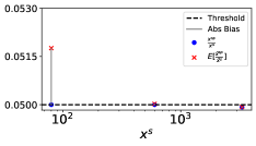
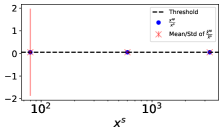
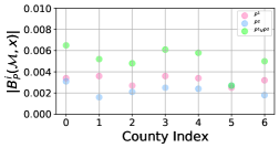
Figure 4: Unfairness effect in ratios (left), thresholding (middle) and predicates disjunction (right)

Ratio Functions

The next result considers ratio functions of the form $P_{i}(\langle x,y\rangle)\!=\!\nicefrac{{x}}{{y}}$ with $x,y\!\in\!\mathbb{R}$ and $x\!\leq\!y$, which occur in the Minority language voting right benefits problem $P_{i}^{M}$. In the following $\mathcal{M}$ is the Laplace mechanism.

Corollary 5.

Mechanism $\mathcal{M}$ is not fair w.r.t. $P_{i}(\langle x,y\rangle)=\nicefrac{{x}}{{y}}$ and inputs $x,y$.

The above is a direct consequence of Corollary 4.

Figure 4 (left) provides an illustration linked to problem $P^{M}$. It shows the original values $\nicefrac{{x^{sp}}}{{x^{s}}}$ (blue circles) and the expected values of the privacy-preserving counterparts (red crosses) of three counties; from left to right: Loving county, TX, where $\nicefrac{{x^{sp}}}{{x^{s}}}\!=\!\nicefrac{{4}}{{80}}\!=\!0.05$, Terrell county, TX, where $\nicefrac{{x^{sp}}}{{x^{s}}}\!=\!\nicefrac{{30}}{{600}}\!=\!0.05$, and Union county, NM, where $\nicefrac{{x^{sp}}}{{x^{s}}}\!=\!\nicefrac{{160}}{{3305}}\!=\!0.0484$. The length of the gray vertical line represents the absolute bias and the dotted line marks a threshold value ($0.05$) associated with the formula $P^{M}_{i}$. While the three counties have (almost) identical ratios values, they induce significant differences in absolute bias. This is due to the difference in scale of the numerator (and denominator), with smaller numerators inducing higher bias.

Thresholding Functions

As discussed in Theorem 4, discontinuities caused by indicator functions, including thresholding, may induce unfairness. This is showcased in Figure 4 (center) which describes the same setting depicted in Figure  4 (left) but with the red line indicating the variance of the noisy ratios. Notice the significant differences in error variances, with Loving county exhibiting the largest variance. This aspect is also shown in Figure 3 where the counties with ratios lying near the threshold value have higher decisions errors than those whose ratios lies far from it.

6.2 Predicates Composition

The next result highlights the negative impact coming from the composition of Boolean predicates. The following important result is corollary of Theorem 5 and provides a lower bound on the fairness bound.

Corollary 6.

Let mechanism $\mathcal{M}$ be $\alpha_{k}$-fair w.r.t. to problem $P^{k}$ ($k\in\{1,2\}$). Then $\mathcal{M}$ is $\alpha$-fair w.r.t. problems $P=P^{1}\lor P^{2}$ and $P=P^{1}\land P^{2}$, with $\alpha>\max(\alpha_{1},\alpha_{2})$.

Proof.

The proof is provided for $P=P^{1}\lor P^{2}$. The argument for the disjunctive case is similar to the following one.

First the proof shows that $\alpha>\alpha_{1}$. By (10) of Theorem 5, it follows

$$\alpha-\alpha_{1} =\underline{B}^{1}+\alpha_{2}+\underline{B}^{2}-(\alpha_{1}+\underline{B}^{1})(\alpha_{2}\!+\!\underline{B}^{2})\!-\!\underline{B}^{1}\underline{B}^{2}$$ (21a)

$$=\underline{B}^{1}+\alpha_{2}+\underline{B}^{2}-\alpha_{1}\alpha_{2}-\alpha_{1}\underline{B}^{2}-\alpha_{2}\underline{B}^{1}$$ (21b)

$$=\underline{B}^{1}(1-\alpha_{2})+\alpha_{2}(1-\alpha_{1})+\underline{B}^{2}(1-\alpha_{1}).$$ (21c)

Since $\mathcal{M}$ is not trivial (by assumption), we have that $0\leq\alpha_{1},\alpha_{2}<0.5$. Thus:

$$\underline{B}^{1}(1-\alpha_{2})>0$$ (22a)

$$\alpha_{2}(1-\alpha_{1})\geq 0$$ (22b)

$$\underline{B}^{2}(1-\alpha_{1})>0.$$ (22c)

Combining the inequalities in (22) above with Equation 21, results in

$$\alpha-\alpha_{1}>0,$$

which implies that $\alpha>\alpha_{1}$. An analogous argument follows for $\alpha_{2}$. Therefore, $\alpha>\alpha_{1}$ and $\alpha>\alpha_{2}$, which asserts the claim. ∎

Figure 4 (right) illustrates Corollary 6. It once again uses the minority language problem $P^{M}$. In the figure, each dot represents the absolute bias $|B^{i}_{P^{M}}(\mathcal{M},\bm{x})|$ associated with a selected county. Red and blue circles illustrate the absolute bias introduced by mechanism $\mathcal{M}$ for problem $P^{1}(x^{sp})\!=\!\mathbbm{1}\{x^{sp}\!\geq\!10^{4}\}$ and $P^{2}(x^{sp},x^{spe})\!=\!\mathbbm{1}\{\frac{x^{spe}}{x^{sp}}\!>\!0.0131\}$ respectively. The selected counties have all similar and small absolute bias on the two predicates $P^{1}$ and $P^{2}$. However, when they are combined using logical connector $\lor$, the resulting absolute bias increases substantially, as illustrated by the associated green circles.

The following analyzes an interesting difference in errors based on the Truth values of the composing predicates $P^{1}$ and $P^{2}$, and shows that the highest error is achieved when they both are True for $\land$ and when they both are False for $\lor$ connectors. This result may have strong implications in classification tasks.

Theorem 7.

Suppose mechanism $\mathcal{M}$ is fair w.r.t. predicates $P^{1}$ and $P^{2}$, and consider predicate $P=P^{1}\land P^{2}$. Let $|B_{P}(a,b)|$ denote the absolute bias for $\mathcal{M}$ w.r.t. $P$ when predicate $P^{1}=a$ and predicate $P^{1}=b$, for $a,b\in\{\textsl{True},\textsl{False}\}$. Then, $|B_{P}(\textsl{True},\textsl{True})|\geq|B_{P}(a,b)|$ for any other $a,b\in\{\textsl{True},\textsl{False}\}$.

Proof.

Since $\mathcal{M}$ is fair w.r.t. to both predicates $P^{1}$ and $P^{2}$, then, by (consequence of) Corollary 2, $\forall i\in[n]$, $\mathcal{M}$ absolute bias w.r.t.  $P^{1}$ and $P^{2}$ is constant and bounded in $(0,\nicefrac{{1}}{{2}})$:

$$|B^{i}_{P^{1}}|=B_{1}\in(0,0.5);\qquad|B^{i}_{P^{2}}|=B_{2}\in(0,0.5)$$

Given the bound above, by Lemma 1 and for every $x\in\mathcal{X}$, it is possible to derive the following sequence of relations between each combination of predicate truth values:

$$\eqref{lemma1:c4} >\eqref{lemma1:c2};$$ (23a)

$$\eqref{lemma1:c4} >\eqref{lemma1:c3};$$ (23b)

$$\eqref{lemma1:c2} >\eqref{lemma1:c1};$$ (23c)

$$\eqref{lemma1:c3} >\eqref{lemma1:c1},$$ (23d)

It follows immediately that case ((iv)) is the largest among all the other cases, concluding the proof. ∎

Theorem 8.

Suppose mechanism $\mathcal{M}$ is fair w.r.t. predicates $P^{1}$ and $P^{2}$, and consider predicate $P=P^{1}\lor P^{2}$. Let $|B_{P}(a,b)|$ denote the absolute bias for $\mathcal{M}$ w.r.t. $P$ when predicate $P^{1}=a$ and predicate $P^{1}=b$, for $a,b\in\{\textsl{True},\textsl{False}\}$. Then, $|B_{P}(\textsl{False},\textsl{False})|\geq|B_{P}(a,b)|$ for any other $a,b\in\{\textsl{True},\textsl{False}\}$.

The proof follows an analogous argument to that used in the proof of Theorem 7.

Figure 5 illustrates this result on the Minority Language problem, with $P^{1}=\frac{x_{i}^{sp}}{x_{i}^{s}}\!>\!0.05$ $P^{2}=x_{i}^{sp}\!>\!10^{4}$, and $P^{3}=\frac{x_{i}^{spe}}{x_{i}^{sp}}\!>\!0.0131$. It reports the decision errors on the y-axis (absolute bias). Notice that the red group is the most penalized in Figure 5 (left) and the least penalized in Figure 5 (right).

Figure 5: Absolute bias (decision errors) in the Minority Language Problem: The errors are shown for four different groups of data corresponding to predicates $P=P^{1}\lor P^{2}$ (left) and $P=P^{1}\land P^{3}$ (right)

6.3 Post-Processing

The final analysis of bias relates to the effect of post-processing the output of the differentially private data release. In particular, the section focuses on ensuring non-negativity of the released data. The discussion focuses on problem $P^{F}$ but the results are, once again, general.

The section first presents a negative result: the application of a post-processing operator

$$\text{PP}^{\geq\ell}(z)\stackrel{{\scriptstyle\text{def}}}{{=}}\max(\ell,z)$$

to ensure that the result is at least $\ell$ induces a positive bias which, in turn, can exacerbate the disparity error of the allotment problem.

Theorem 9.

Let $\tilde{x}=x+\textrm{Lap}(\lambda)$, with scale $\lambda>0$, and $\hat{x}=\text{PP}^{\geq\ell}(\tilde{x})$, with $\ell<x$, be its post-processed value. Then,

$$\mathbb{E}[\hat{x}]=x+\frac{\lambda}{2}\exp(\frac{\ell-x}{\lambda}).$$

Proof.

The expectation of the post-processed value $\hat{x}$ is given by:

$$E[\hat{x}] =\int_{-\infty}^{\infty}\!\!\max(\ell,\tilde{x})p(\tilde{x})\;d\tilde{x}$$ (24a)

$$=\int_{-\infty}^{\ell}\!\!\max(\ell,\tilde{x})p(\tilde{x})\;d\tilde{x}+\int_{\ell}^{x}\!\!\max(\ell,\tilde{x})p(\tilde{x})\;d\tilde{x}+\int_{x}^{\infty}\!\!\max(\ell,\tilde{x})p(\tilde{x})\;d\tilde{x},$$ (24b)

where $p(\tilde{x})=\nicefrac{{1}}{{2\lambda}}\exp(-\nicefrac{{|\tilde{x}-x|}}{{\lambda}})$ is the pdf of Laplace. The following computes separately the three terms in Equation 24b:

$$\int_{-\infty}^{\ell}\!\!\max(\ell,\tilde{x})p(\tilde{x})\;d\tilde{x} =\int_{-\infty}^{\ell}\!\!\ell\,p(\tilde{x})\;d\tilde{x}=\ell\int_{-\infty}^{\ell}\!\!p(\tilde{x})\;d\tilde{x}=\frac{1}{2}\ell\exp(\frac{\ell-x}{\lambda})$$ (25)

$$\int_{\ell}^{x}\!\!\max(\ell,\tilde{x})p(\tilde{x})\;d\tilde{x} =\int_{\ell}^{x}\!\!\tilde{x}p(\tilde{x})\;d\tilde{x}=\frac{1}{2}(x-\lambda)-\frac{1}{2}(\ell-\lambda)\exp(\frac{\ell-x}{\lambda})$$ (26)

$$\int_{x}^{\infty}\!\!\max(\ell,\tilde{x})p(\tilde{x})\;d\tilde{x} =\int_{x}^{\infty}\!\!\tilde{x}p(\tilde{x})\;d\tilde{x}=\frac{1}{2}(x+\lambda).$$ (27)

Combining equations (25)–(27) with (24b), gives

$$E[\hat{x}]=x+\frac{\lambda}{2}\exp(\frac{\ell-x}{\lambda}).$$

∎

Lemma 9 indicates the presence of positive bias of post-processed Laplace random variable when ensuring non-negativity, and that such bias is $B^{i}(\mathcal{M},\bm{x})=\mathbb{E}[\hat{x_{i}}]-x_{i}=\exp(\frac{\ell-x_{i}}{\lambda})\leq\nicefrac{{\lambda}}{{2}}$ for $\ell\leq x_{i}$. As shown in Figure 2 the effect of this bias has a negative impact on the final disparity of the allotment problem, where smaller entities have the largest bias (in the Figure $\ell=0$).

The remainder of the section discusses positive results for two additional classes of post-processing: (1) The integrality constraint program $\text{PP}^{\mathbb{N}}(z)$, which enforces the integrality of the released values, and (2) The sum-constrained constrained program $\text{PP}^{\sum_{S}}(z)$, which enforces a linear constraint on the data. The following results show that these post-processing steps do not contribute to further biasing the decisions.

Integrality Post-processing

The integrality post-processing $\text{PP}^{\mathbb{N}}(z)$ is used when the released data are integral quantities. The following post-processing step, based on stochastic rounding produces integral quantities:

$$\text{PP}^{\mathbb{N}}(z)=\begin{cases}\lfloor z\rfloor\ \mbox{w.p.:}\ 1-(z-\lfloor z\rfloor)\\ \lfloor z\rfloor+1\ \ \mbox{w.p.:}\ z-\lfloor z\rfloor\end{cases}$$ (28)

It is straightforward to see that the above is an unbias estimator: $\mathbb{E}[\text{PP}^{\mathbb{N}}(\tilde{x})]=\tilde{x}$ and thus, no it introduces no additional bias to $\text{PP}^{\mathbb{N}}(\tilde{x})$.

Sum-constrained Post-processing

The sum-constrained post-processing $\text{PP}^{\sum_{S}}(z)$ is expressed through the following constrained optimization problem:

$$\min_{\hat{z}}\left\|\hat{z}-z\right\|^{2}_{2}\\ \ \mbox{s.t}:\ \bm{1}^{T}z=S$$ (29)

This class of constraints is typically enforced when the private outcomes are required to match some fixed resource to distribute. For example, the outputs of the allotment problem $P^{F}$ should be such that the total budget is allotted, and thus $\sum_{i}P^{F}_{i}(\tilde{x})=1$.

Theorem 10.

Consider an $\alpha$-fair mechanism $\mathcal{M}$ w.r.t. problem $P$. Then $\mathcal{M}$ is also $\alpha$-fair w.r.t. problem $\text{PP}^{\sum_{S}}(P)$.

The following relies on a result by Zhu et al. [26].

Proof.

Denote $z_{i}$ and $\hat{z}_{i}$ as for $=P_{i}(\bm{\tilde{x}})$ and $\text{PP}^{\sum_{S}}(z_{i})$, respectively. Note that problem (29) is convex and its unique minimizer is $\hat{z}_{i}=z_{i}+\eta$ with $\eta=\frac{S-\sum_{i}z_{i}}{n}$. Its expected value is:

$$\mathbb{E}[\hat{z}_{i}] =\mathbb{E}[z_{i}+\eta]=\mathbb{E}\left[z_{i}+\frac{S-\sum_{j\neq i}z_{j}}{n}\right]$$ (30a)

$$=\frac{n-1}{n}\mathbb{E}\left[z_{i}\right]-\frac{1}{n}\sum_{j\neq i}\mathbb{E}\left[z_{j}\right]+\frac{S}{n}$$ (30b)

$$=\frac{n-1}{n}\left(z_{i}+B^{i}_{P}\right)-\frac{1}{n}\left(\sum_{j\neq i}z_{j}+B^{j}_{P}\right)+\frac{S}{n}$$ (30c)

$$=\frac{n-1}{n}\left(z_{i}+B^{i}_{P}\right)-\frac{1}{n}\left(S-z_{i}+\sum_{j\neq i}B^{j}_{P}\right)+\frac{S}{n}$$ (30d)

$$=z_{i}+\frac{\sum_{j\neq i}\left(B^{i}_{P}-B^{j}_{P}\right)}{n}.$$ (30e)

The above follows from linearity of expectation and the last equality indicates that the bias of entity $i$ under sum-constrained post-processing is $B^{i}_{\text{PP}^{\sum_{S}}(P)}=\frac{\sum_{j\neq i}(B^{i}_{P}-B^{j}_{P})}{n}$. Thus, the fairness bound $\alpha^{\prime}$ attained after post-processing is:

$$\alpha^{\prime} =\max_{i,k}\left|B^{i}_{\text{PP}^{\sum_{S}}(P)}-B^{k}_{\text{PP}^{\sum_{S}}(P)}\right|$$ (31a)

$$=\max_{i,k}\frac{\sum_{j\neq i}(B^{i}_{P}-B^{j}_{P})}{n}-\frac{\sum_{j\neq k}(B^{k}_{P}-B^{j}_{P})}{n}$$ (31b)

$$=\max_{i,k}|B^{i}_{P}-B^{k}_{P}|=\alpha$$ (31c)

Therefore, the sum-constrained post-processing does not introduce additional unfairness to mechanism $\mathcal{M}$. ∎

Discussion

The results highlighted in this section are both surprising and significant. They show that the motivating allotment problems and decision rules induce inherent unfairness when given as input differentially private data. This is remarkable since the resulting decisions have significant societal, economic, and political impact on the involved individuals: federal funds, vaccines, and therapeutics may be unfairly allocated, minority language voters may be disenfranchised, and congressional apportionment may not be fairly reflected. The next section identifies a set of guidelines to mitigate these negative effects.

7 Mitigating Solutions

7.1 The Output Perturbation Approach

This section proposes three guidelines that may be adopted to mitigate the unfairness effects presented in the paper, with focus on the motivating allotments problems and decision rules.

A simple approach to mitigate the fairness issues discussed is to recur to output perturbation to randomize the outputs of problem $P_{i}$, rather than its inputs, using an unbiased mechanism. Injecting noise directly after the computation of the outputs $P_{i}(\bm{x})$, ensures that the result will be unbiased. However, this approach has two shortcomings. First, it is not applicable to the context studied in this paper, where a data agency desires to release a privacy-preserving data set $\tilde{\bm{x}}$ that may be used for various decision problems. Second, computing the sensitivity of the problem $P_{i}$ may be hard, it may require to use a conservative estimate, or may even be impossible, if the problem has unbounded range. A conservative sensitivity implies the introduction of significant loss in accuracy, which may render the decisions unusable in practice.

7.2 Linearization by Redundant Releases

A different approach considers modifying on the decision problem $P_{i}$ itself. Many decision rules and allotment problems are designed in an ad-hoc manner to satisfy some property on the original data, e.g., about the percentage of population required to have a certain level of education. Motivated by Corollaries 1 and 2, this section proposes guidelines to modify the original problem $P_{i}$ with the goal of reducing the unfairness effects introduced by differential privacy.

The idea is to use a linearized version $\bar{P}_{i}$ of problem $P_{i}$. While many linearizion techniques exists [18], and are often problem specific, the section focuses on a linear proxy $\bar{P}_{i}^{F}$ to problem $P^{F}_{i}$ that can be obtained by enforcing a redundant data release. While the discussion focuses on problem $P^{F}_{i}$, the guideline is general and applies to any allotment problem with similar structure.

Let $Z=\sum_{i}a_{i}x_{i}$. Problem $P^{F}_{i}(\bm{x})\!=\!\nicefrac{{a_{i}x_{i}}}{{Z}}$ is linear w.r.t. the inputs $x_{i}$ but non-linear w.r.t. $Z$. However, releasing $Z$, in addition to releasing the privacy-preserving values $\tilde{\bm{x}}$, would render $Z$ a constant rather than a problem input to $P^{F}$. To do so, $Z$ can either be released publicly, at cost of a (typically small) privacy leakage or by perturbing it with fixed noise. The resulting linear proxy allocation problem $\bar{P}^{F}_{i}$ is thus linear in the inputs $\bm{x}$.

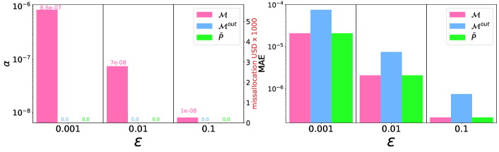
Figure 6: Linearization by redundant release: Fairness and error comparison.

Figure 6 illustrates this approach in practice. The left plot shows the fairness bound $\alpha$ and the right plot shows the empirical mean absolute error $\frac{1}{m}\sum_{k=1}^{m}|P_{i}(\bm{x}^{k})-P_{i}(\tilde{\bm{x}}^{m})|$, obtained using $m=10^{4}$ repetitions, when the DP data $\tilde{\bm{x}}$ is applied to (1) the original problem $P$, (2) its linear proxy $\bar{P}$, and (3) when output perturbation (denoted $\mathcal{M}^{\text{out}}$) is adopted. The number on top of each bar reports the fairness bounds, and emphasize that the proposed remedy solutions achieve perfect-fairness. Notice that the proposed linear proxy solution can reduce the fairness violation dramatically while retaining similar errors. While the output perturbation method reduces the disparity error, it also incurs significant errors that make the approach rarely usable in practice.

Learning Piece-wise Linear proxy-functions

Due to the discontinuities arising in decision rules (see for example problem $\eqref{p:coverage}$), it is substantially more challenging to develop mitigation strategies than in allotment problems. In particular, the discontinuities present in problem $P^{M}$ render the use of linear proxies ineffective.

The following strategy combines two ideas: (1) partitioning, in a privacy-preserving fashion, the original problem into subproblems that are locally continuous and amenable to linearizations with low accuracy loss, and (2) the systematic learning of linear proxies. More precisely, the idea is to partition the input values $\bm{x}$ into several groups $\bm{x}_{1},\ldots\bm{x}_{G}$ (e.g., individuals from the same state or from states of similar magnitude) and to approximate subproblem $P^{M}_{i}(\bm{x}_{k})$ with a linear proxy $\bar{P}^{M}_{i}(\bm{x}_{k})$ for each group $k\in[G]$. The resulting problem $\bar{P}^{M}_{i}$ then becomes a piecewise linear function that approximates the original problem $P^{M}_{i}$.

Rather than using an ad-hoc method to linearize problem $P^{M}$, the paper proposes to obtain it by fitting a linear model to the data $\bm{x}_{k}$ of each group $k\in[G]$. Figure 7 presents results for problem $P^{M}$. Each subgroup is trained using features $\{x^{spe},x^{sp},x^{s}\}$ and the resulting model coefficients are used to construct the proxy linear function for the subproblems $\bar{P}^{M}_{i}(\bm{x}_{G})$. The results use the value $x^{sp}$ to partition the dataset into $9$ groups of approximately equal size. To ensure privacy, the grouping is executed using privacy-preserving $x^{sp}$ values. Figure 7 compares the original problem $P$, a proxy-model $\bar{P}_{LR}$ whose pieces are learned using linear regression (LR), and a proxy model $\bar{P}_{SVM}$ whose pieces are learned using a linear SVM model. All three problems take as input the private data $\tilde{\bm{x}}$ and are compared with the original version of the problem $P$. The x-axis shows the range of $x^{sp}$ that defines the partition, while the y-axis shows the fairness bound $\alpha$ computed within each group. The positive effects of the proposed piecewise linear proxy problem are dramatic. The fairness violations decrease significantly when compared to those obtained by the original model. the fairness violation of the SVM model is typically lower than that obtained by the LR model, and this may be due to the accuracy of the resulting model – with SVM reaching higher accuracy than LR in our experiments. Finally, as the population size increases, the fairness bound $\alpha$ decreases and emphasizes further the largest negative impact of the noise on the smaller counties.

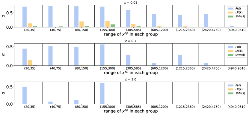
Figure 7: Linearization by redundant release: Fairness comparison.

It is important to note that the experiments above use a data release mechanism $\mathcal{M}$ that applies no post-processing. A discussion about the mitigating solutions for the bias effects caused by post-processing is presented next.

7.3 Modified Post-Processing

This section introduces a simple, yet effective, solution to mitigate the negative fairness impact of the non-negative post-processing. The proposed solution operates in 3 steps: It first (1) performs a non-negative post-processing of the privacy-preserving input $\tilde{x}$ to obtain value $\bar{x}\!=\!\text{PP}^{\geq\ell}(\tilde{x})$. Next, (2) it computes $\bar{x}_{T}\!=\!\bar{x}\!-\!\frac{T}{\bar{x}+1-\ell}$. Its goal is to correct the error introduced by the post-processing operator, which is especially large for quantities near the boundary $\ell$. Here $T$ is a temperature parameter that controls the strengths of the correction. This step reduces the value $\bar{x}$ by quantity $\frac{T}{\bar{x}+1-\ell}$. The effect of this operation is to reduce the expected value $\mathbb{E}[\bar{x}]$ by larger (smaller) amounts as $x$ get closer (farther) to the boundary value $\ell$. Finally, (3) it ensures that the final estimate is indeed lower bounded by $\ell$, by computing $\hat{x}=\max(\bar{x}_{T},\ell)$.

The benefits of this approach are illustrated in Figure 8, which show the absolute bias $|B^{i}_{P^{F}}|$ for the Title 1 fund allocation problem that is induced by the original mechanism $\mathcal{M}$ with standard post-processing $\text{PP}^{\geq 0}$ and by the proposed modified post-processing for different temperature values $T$.

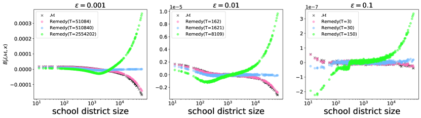
Figure 8: Modified post-processing: Unfairness reduction.

The figure illustrates the role of the temperature $T$ in the disparity errors. Small values $T$ may have small impacts in reducing the disparity errors, while large $T$ values can introduce errors, thus may exacerbate unfairness. The optimal choice for $T$ can be found by solving the following:

$$T^{*}=\operatorname*{argmin}_{T}\big{(}\max_{\bm{x}\geq\ell}|\mathbb{E}[\hat{\bm{x}}_{T}]-\bm{x}|-\min_{\bm{x}\geq\ell}|\mathbb{E}[\hat{\bm{x}}_{T}]-\bm{x}|\big{)},$$ (32)

where $\hat{\bm{x}}_{T}$ is a random variable obtained by the proposed 3 step solution, with temperature $T$. The expected value of $\hat{\bm{x}}$ can be approximated via sampling. Note that naively finding the optimal $T$ may require access to the true data. Solving the problem above in a privacy-preserving way is beyond the scope of the paper and the subject of future work.

The reductions in the fairness bound $\alpha$ for problem $P^{F}$ are reported in Figure 9 (left), while Figure 9 (right) shows that this method has no perceptible impact on the mean absolute error. Once again, these errors are computed via sampling and use $10^{4}$ samples.

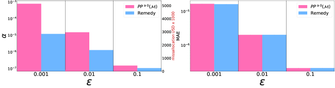
Figure 9: Modified post-processing on problem $P^{F}$.

7.4 Fairness Payment

Finally, this section focuses on allotment problems, like $P^{F}$, that distribute a budget $B$ among $n$ entities, and where the allotment for entity $i$ represents the fraction of budget $B$ it expects. Differential privacy typically implements a postprocessing step to renormalize the fractions so that they sum to 1. This normalization, together with nonnegativity constraints, introduces a bias and hence more unfairness. One way to alleviate this problem is to increase the total budget $B$, and avoiding the normalization. This section quantifies the cost of doing so: it defines the cost of privacy, which is the increase in budget $B^{+}$ required to achieve this goal.

Definition 4 (Cost of Privacy).

Given problem $P$, that distributes budget $B$ among $n$ entities, data release mechanism $\mathcal{M}$, and dataset $\bm{x}$, the cost of privacy is:

$$B^{+}=\textstyle\sum_{i\in I^{-}}|B^{i}_{P}(\mathcal{M},\bm{x})|\times B$$

with $I^{-}=\{i\,:\,B^{i}_{P}(\mathcal{M},\bm{x})<0\}$.

Figure 10 illustrates the cost of privacy, in USD, required to render each county in the state of New York not negatively penalized by the effects of differential privacy. The figure shows, in decreasing order, the different costs associated with a mechanism $P^{F}(\text{PP}^{\geq 0}(\bm{x}))$ that applies a post-processing step, one $P^{F}(\bm{x})$ that does not apply post-processing, and one that uses a linear proxy problem $\bar{P}^{F}(\bm{x})$.

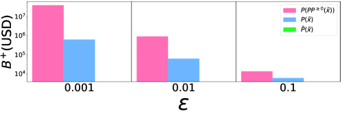
Figure 10: Cost of privacy on problem $P^{F}$.

8 Related Work

The literature on DP and algorithmic fairness is extensive and the reader is referred to, respectively, [7, 25, 8] and [4, 17] for surveys on these topics. However, privacy and fairness have been studied mostly in isolation with a few exceptions. Cummings et al. [5] consider the tradeoffs arising between differential privacy and equal opportunity, a fairness concept that requires a classifier to produce equal true positive rates across different groups. They show that there exists no classifier that simultaneously achieves $(\epsilon,0)$-differential privacy, satisfies equal opportunity, and has accuracy better than a constant classifier. Ekstrand et al. [9] raise questions about the tradeoffs involved between privacy and fairness, and Jagielski et al. [13] shows two algorithms that satisfy $(\epsilon,\delta)$-differential privacy and equalized odds. Although it may sound like these algorithms contradict the impossibility result from [5], it is important to note that they are not considering an $(\epsilon,0)$-differential privacy setting. Tran et al. [23] developed a differentially private learning approach to enforce several group fairness notions using a Lagrangian dual method. Zhu et al. [27] studied the bias and variance induced by several important classes of post-processing and that the resulting bias can also have some disproportionate impact on the outputs. Pujol et al. [16] were seemingly first to show, empirically, that there might be privacy-fairness tradeoffs involved in resource allocation settings. In particular, for census data, they show that the noise added to achieve differential privacy could disproportionately affect some groups over others. This paper builds on these empirical observations and provides a step towards a deeper understanding of the fairness issues arising when differentially private data is used as input to decision problems. This work is an extended version of [24].

9 Conclusions

This paper analyzed the disparity arising in decisions granting benefits or privileges to groups of people when these decisions are made adopting differentially private statistics about these groups. It first characterized the conditions for which allotment problems achieve finite fairness violations and bound the fairness violations induced by important components of decision rules, including reasoning about the composition of Boolean predicates under logical operators. Then, the paper analyzed the reasons for disparity errors arising in the motivating problems and recognized the problem structure, the predicate composition, and the mechanism post-processing, as paramount to the bias and unfairness contribution. Finally, it suggested guidelines to act on the decision problems or on the mechanism (i.e., via modified post-processing steps) to mitigate the unfairness issues. The analysis provided in this paper may provide useful guidelines for policy-makers and data agencies for testing the fairness and bias impacts of privacy-preserving decision making.

Appendix A Missing Proofs

Proof of Lemma 1.

The proof proceeds by cases.
Case (i): $P^{1}_{i}(\bm{x})=\textsl{False};P^{2}_{i}(\bm{x})=\textsl{False}$, therefore $P_{i}(\bm{x})=P^{1}_{i}(\bm{x})\land P^{2}_{i}(\bm{x})=\textsl{False}$ and,

$$\text{Pr}\left(P_{i}(\tilde{\bm{x}})\neq P_{i}(\bm{x})\right) =\text{Pr}\left(P^{1}_{i}(\tilde{\bm{x}})\land P^{2}_{i}(\tilde{\bm{x}})\neq\textsl{False}\right)$$ (33a)

$$=\text{Pr}\left(P^{1}_{i}(\tilde{\bm{x}})\land P^{2}_{i}(\tilde{\bm{x}})=\textsl{True}\right)$$ (33b)

$$=\text{Pr}\left(P^{1}_{i}(\tilde{\bm{x}})=\textsl{True}\land P^{2}_{i}(\tilde{\bm{x}})=\textsl{True}\right)$$ (33c)

$$=\text{Pr}\left(P^{1}_{i}(\tilde{\bm{x}})=\textsl{True}\right)\cdot\text{Pr}\left(P^{2}_{i}(\tilde{\bm{x}})=\textsl{True})\right)$$ (33d)

$$=\text{Pr}\left(P^{1}_{i}(\tilde{\bm{x}})\neq P^{1}_{i}(\bm{x})\right)\cdot\text{Pr}\left(P^{2}_{i}(\tilde{\bm{x}})\neq P^{2}_{i}(\bm{x})\right)$$ (33e)

$$=|B^{i}_{P^{1}}||B^{i}_{P^{2}}|$$ (33f)

Where equation (33d) is due to $P^{1}_{i}\mathchoice{\mathrel{\hbox to0.0pt{$\displaystyle\perp$\hss}\mkern 2.0mu{\displaystyle\perp}}}{\mathrel{\hbox to0.0pt{$\textstyle\perp$\hss}\mkern 2.0mu{\textstyle\perp}}}{\mathrel{\hbox to0.0pt{$\scriptstyle\perp$\hss}\mkern 2.0mu{\scriptstyle\perp}}}{\mathrel{\hbox to0.0pt{$\scriptscriptstyle\perp$\hss}\mkern 2.0mu{\scriptscriptstyle\perp}}}P^{2}_{i}$.

Case (ii): $P^{1}_{i}(\bm{x})=\textsl{False};P^{2}_{i}(\bm{x})=\textsl{True}$, therefore $P_{i}(\bm{x})=P^{1}_{i}(\bm{x})\land P^{2}_{i}(\bm{x})=\textsl{False}$, and

$$\text{Pr}\left(P_{i}(\tilde{\bm{x}})\neq P_{i}(\bm{x})\right) =\text{Pr}\left(P^{1}_{i}(\tilde{\bm{x}})\land P^{2}_{i}(\tilde{\bm{x}})\neq\textsl{False}\right)$$ (34a)

$$=\text{Pr}\left(P^{1}_{i}(\tilde{\bm{x}})\land P^{2}_{i}(\tilde{\bm{x}})=\textsl{True}\right)$$ (34b)

$$=\text{Pr}\left(P^{1}_{i}(\tilde{\bm{x}})=\textsl{True}\land P^{2}_{i}(\tilde{\bm{x}})=\textsl{True}\right)$$ (34c)

$$=\text{Pr}\left(P^{1}_{i}(\tilde{\bm{x}})=\textsl{True})\right)\cdot\text{Pr}\left(P^{2}_{i}(\tilde{\bm{x}})=\textsl{True})\right)$$ (34d)

$$=\text{Pr}\left(P^{1}_{i}(\tilde{\bm{x}})\neq P^{1}_{i}(\bm{x})\right)\cdot\text{Pr}\left(P^{2}_{i}(\tilde{\bm{x}})=P^{2}_{i}(\bm{x})\right)$$ (34e)

$$=\text{Pr}\left(P^{1}_{i}(\tilde{\bm{x}})\neq P^{1}_{i}(\bm{x})\right)\cdot\left(1-\text{Pr}\left(P^{2}_{i}(\tilde{\bm{x}})\neq P^{2}_{i}(\bm{x})\right)\right)$$ (34f)

$$=|B^{i}_{P^{1}}|\left(1-|B^{i}_{P^{2}}|\right)$$ (34g)

Where equation (34e) is due to $P^{1}_{i}\mathchoice{\mathrel{\hbox to0.0pt{$\displaystyle\perp$\hss}\mkern 2.0mu{\displaystyle\perp}}}{\mathrel{\hbox to0.0pt{$\textstyle\perp$\hss}\mkern 2.0mu{\textstyle\perp}}}{\mathrel{\hbox to0.0pt{$\scriptstyle\perp$\hss}\mkern 2.0mu{\scriptstyle\perp}}}{\mathrel{\hbox to0.0pt{$\scriptscriptstyle\perp$\hss}\mkern 2.0mu{\scriptscriptstyle\perp}}}P^{2}_{i}$.

Case (iii): $P^{1}_{i}(\bm{x})=\textsl{True};P^{2}_{i}(\bm{x})=\textsl{False}$, therefore $P_{i}(\bm{x}))=P^{1}_{i}(\bm{x})\land P^{2}_{i}(\bm{x})=\textsl{False}$, and

$$\text{Pr}\left(P_{i}(\tilde{\bm{x}})\neq P_{i}(\bm{x})\right) =\text{Pr}\left(P^{1}_{i}(\tilde{\bm{x}})\land P^{2}_{i}(\tilde{\bm{x}})\neq\textsl{False}\right)$$ (35a)

$$=\text{Pr}\left(P^{1}_{i}(\tilde{\bm{x}})\land P^{2}_{i}(\tilde{\bm{x}})=\textsl{True}\right)$$ (35b)

$$=\text{Pr}\left(P^{1}_{i}(\tilde{\bm{x}})=\textsl{True}\land P^{2}_{i}(\tilde{\bm{x}})=\textsl{True}\right)$$ (35c)

$$=\text{Pr}\left(P^{1}_{i}(\tilde{\bm{x}})=\textsl{True}\right)\cdot\text{Pr}\left(P^{2}_{i}(\tilde{\bm{x}})=\textsl{True}\right)$$ (35d)

$$=\text{Pr}\left(P^{1}_{i}(\tilde{\bm{x}})=P^{1}_{i}(\bm{x})\right)\cdot\text{Pr}\left(P^{2}_{i}(\tilde{\bm{x}})\neq P^{2}_{i}(\bm{x})\right)$$ (35e)

$$=\left(1-\text{Pr}\left(P^{1}_{i}(\tilde{\bm{x}})\neq P^{1}_{i}(\bm{x})\right)\right)\cdot\text{Pr}\left(P^{2}_{i}(\tilde{\bm{x}})\neq P^{2}_{i}(\bm{x})\right)$$ (35f)

$$=\left(1-|B^{i}_{P^{1}}|\right)|B^{i}_{P^{2}}|$$ (35g)

Where equation (35d) is due to $P^{1}_{i}\mathchoice{\mathrel{\hbox to0.0pt{$\displaystyle\perp$\hss}\mkern 2.0mu{\displaystyle\perp}}}{\mathrel{\hbox to0.0pt{$\textstyle\perp$\hss}\mkern 2.0mu{\textstyle\perp}}}{\mathrel{\hbox to0.0pt{$\scriptstyle\perp$\hss}\mkern 2.0mu{\scriptstyle\perp}}}{\mathrel{\hbox to0.0pt{$\scriptscriptstyle\perp$\hss}\mkern 2.0mu{\scriptscriptstyle\perp}}}P^{2}_{i}$.

Case (iv): $P^{1}_{i}(\bm{x})=\textsl{True};P^{2}_{i}(\bm{x})=\textsl{True}$, therefore $P_{i}(\bm{x})=P^{1}_{i}(\bm{x})\land P^{2}_{i}(\bm{x})=\textsl{True}$, and

$$\text{Pr}\left(P_{i}(\tilde{\bm{x}})\neq P_{i}(\bm{x})\right) =\text{Pr}\left(P^{1}_{i}(\tilde{\bm{x}})\land P^{2}_{i}(\tilde{\bm{x}})\neq\textsl{True}\right)$$ (36a)

$$=\text{Pr}\left(P^{1}_{i}(\tilde{\bm{x}})\land P^{2}_{i}(\tilde{\bm{x}})=\textsl{False}\right)$$ (36b)

$$=1-\text{Pr}\left(P^{1}_{i}(\tilde{\bm{x}})=\textsl{True}\land P^{2}_{i}(\tilde{\bm{x}})=\textsl{True}\right)$$ (36c)

$$=1-\text{Pr}\left(P^{1}_{i}(\tilde{\bm{x}})=\textsl{True}\right)\text{Pr}\left(P^{2}_{i}(\tilde{\bm{x}})=\textsl{True}\right)$$ (36d)

$$=1-\left(1-\text{Pr}\left(P^{1}_{i}(\tilde{\bm{x}})\neq P^{1}_{i}(\bm{x})\right)\right)\left(1-\text{Pr}\left(P^{2}_{i}(\tilde{\bm{x}})\neq P^{2}_{i}(\bm{x})\right)\right)$$ (36e)

$$=1-\left(1-|B^{i}_{P^{1}}|\right)\left(1-|B^{i}_{P^{2}}|\right)$$ (36f)

$$=|B^{i}_{P^{1}}|+|B^{i}_{P^{2}}|-|B^{i}_{P^{1}}||B^{i}_{P^{2}}|$$ (36g)

Where equation (36d) is due to $P^{1}_{i}\mathchoice{\mathrel{\hbox to0.0pt{$\displaystyle\perp$\hss}\mkern 2.0mu{\displaystyle\perp}}}{\mathrel{\hbox to0.0pt{$\textstyle\perp$\hss}\mkern 2.0mu{\textstyle\perp}}}{\mathrel{\hbox to0.0pt{$\scriptstyle\perp$\hss}\mkern 2.0mu{\scriptstyle\perp}}}{\mathrel{\hbox to0.0pt{$\scriptscriptstyle\perp$\hss}\mkern 2.0mu{\scriptscriptstyle\perp}}}P^{2}_{i}$. ∎

Proof of Lemma 2.

The proof is similar to proof of Lemma 1. ∎

Proof of Lemma 3.

The following hold for all four combination of binary boolean values for $P^{1}_{i}(\bm{x})_{i},P^{2}_{i}(\bm{x})\in\{\textsl{False},\textsl{True}\}$:

$$\text{Pr}\left(P_{i}(\tilde{\bm{x}})\neq P_{i}(\bm{x})\right)= \text{Pr}\left(P^{1}_{i}(\tilde{\bm{x}})\oplus P^{2}_{i}(\tilde{\bm{x}})\neq P^{1}_{i}(\bm{x})\oplus P^{2}_{i}(\bm{x})\right)$$

$$= 1-\text{Pr}\left(P^{1}_{i}(\tilde{\bm{x}})=P^{1}_{i}(\bm{x})\right)\cdot\text{Pr}\left(P^{2}_{i}(\tilde{\bm{x}})=P^{2}_{i}(\bm{x})\right)$$

$$- \text{Pr}\left(P^{1}_{i}(\tilde{\bm{x}})\neq P^{1}_{i}(\bm{x})\right)\cdot\text{Pr}\left(P^{2}_{i}(\tilde{\bm{x}})\neq P^{2}_{i}(\bm{x})\right)$$

$$= 1-|B^{i}_{P^{1}}||B^{i}_{P^{2}}|-(1-|B^{i}_{P^{1}}|)(1-|B^{i}_{P^{2}}|)$$

$$= |B^{i}_{P^{1}}|+|B^{i}_{P^{2}}|-2|B^{i}_{P^{1}}||B^{i}_{P^{2}}|.$$

Where the second equality is due to $P^{1}_{i}\mathchoice{\mathrel{\hbox to0.0pt{$\displaystyle\perp$\hss}\mkern 2.0mu{\displaystyle\perp}}}{\mathrel{\hbox to0.0pt{$\textstyle\perp$\hss}\mkern 2.0mu{\textstyle\perp}}}{\mathrel{\hbox to0.0pt{$\scriptstyle\perp$\hss}\mkern 2.0mu{\scriptstyle\perp}}}{\mathrel{\hbox to0.0pt{$\scriptscriptstyle\perp$\hss}\mkern 2.0mu{\scriptscriptstyle\perp}}}P^{2}_{i}$. ∎

Appendix B Experimental Details

B.1 General Settings

All experimental codes were written in Python 3.7. Some heavy computation tasks were performed on a cluster equipped with Intel(R) Xeon(R) Platinum 8260 CPU @ 2.40GHz and 8GB of RAM. We will release our codes upon paper’s acceptance.

B.2 Datasets

Title 1 School Allocation

The dataset was uploaded as a supplemental materials of [3]. The dataset can be downloaded directly from https://tinyurl.com/y6adjsyn.

We processed the dataset by removing schools which contains NULL information, and keeping school districts with at least 1 students. The post-processed dataset left with 16441 school districts.

Minority language voting right benefits

The dataset can be downloaded from https://tinyurl.com/y2244gbt.

The focus of the experiments is on Hispanic groups, which represent the largest minority population. There are 2774 counties that contain at least a Hispanic person.

B.3 Mechanism Implementation

Linear Proxy Allocation $\bar{P}^{F}$

The linear proxy allocation method used for problem $\bar{P}^{F}$ is implement so that, for a given privacy parameter $\epsilon$, the algorithm allocates $\epsilon_{1}=\frac{\epsilon}{2}$ to release the normalization term $Z$. The remaining $\epsilon_{2}=\frac{\epsilon}{2}$ budget is used to publish the population counts $x_{i}$.

Output Perturbation mechanism

The paper uses standard Laplace mechanism: $\tilde{P}^{F}_{i}(\bm{x})=P_{i}(x)+\mbox{Lap}(0,\frac{\Delta}{\epsilon})$. Therein, the global sensitivity $\Delta$ is obtained from Theorem 11. The experiments set a known public lower bound $L=0.9Z$ for the normalization term $Z$ in Theorem 11.

Theorem 11.

Denote $a_{\max}=\max_{i}a_{i}$, and let $L\leq\sum_{i\in[n]}x_{i}a_{i}$ is a known public lower bound for the normalization term. The $l_{1}$ global sensitivity of the query $P^{F}=\{P^{F}_{i}\}^{n}_{i=1}$ with $P^{F}_{i}=\big{(}\frac{x_{i}a_{i}}{\sum_{i\in[n]}x_{i}a_{i}}\big{)}$ is given by:

$$\Delta=\max_{\bm{x},\bm{x^{\prime}}}\left|P^{F}(\bm{x})-P^{F}(\bm{x^{\prime}})\right|_{1}=\frac{2a_{\max}}{L}$$ (37)

Proof.

Let $\bm{x}^{\prime}$ be a dataset constructed by removing a single individual from $\bm{x}$ and denote with $Z=\sum_{j}x_{j}a_{j}$. It follows that:

$$P^{F}_{k}(\bm{x})-P^{F}_{k}(\bm{x^{\prime}})=\begin{cases}\frac{x_{k}a_{k}}{Z}-\frac{(x_{k}-1)a_{k}}{Z-a_{k}}&\text{ if }k=i\\ \frac{x_{k}a_{k}}{Z}-\frac{x_{k}a_{k}}{Z-a_{k}}&\text{ otherwise}.\end{cases}$$

When $k=i$, it follows that:

$$P^{F}_{i}(\bm{x})-P^{F}_{i}(\bm{x^{\prime}}) =\frac{a_{i}\left(Z-x_{i}a_{i}\right)}{Z(Z-a_{i})}$$ (38a)

$$\leq\frac{a_{i}(Z-a_{i})}{Z(Z-a_{i})}=\frac{a_{i}}{Z}\leq\frac{a_{\max}}{Z}$$ (38b)

$$\leq\frac{a_{\max}}{L}$$ (38c)

The last inequality is due to assumption that $Z=\sum_{j\in[n]}a_{j}\cdot x_{j}\geq L$.

Next, when $k\neq i$:

$$P^{F}_{j}(\bm{x})-P^{F}_{j}(\bm{x^{\prime}})=\frac{-a_{j}x_{j}a_{i}}{Z(Z-a_{i})},$$ (39)

and thus

$$\sum_{j\neq i}\left|P^{F}_{j}(\bm{x})-P^{F}_{j}(\bm{x^{\prime}})\right|=a_{i}\frac{Z-a_{i}x_{i}}{Z(Z-a_{i})}$$ (40a)

$$\leq a_{i}\frac{Z-a_{i}}{Z(Z-a_{i})}=a_{i}\frac{1}{Z}\leq\frac{a_{\max}}{L}$$ (40b)

The bound is obtained by adding Equation (38c) with Equation (40b). ∎

References

• [1] Title 13. Title 13, u.s. code. www.census.gov/history/www/reference/privacy_confidentiality/title_13_us_code.html, 2006. Accessed: 2021-01-15.
• [2] John M Abowd. The us census bureau adopts differential privacy. In Proceedings of the 24th ACM SIGKDD International Conference on Knowledge Discovery & Data Mining, pages 2867–2867, 2018.
• [3] John M Abowd and Ian M Schmutte. An economic analysis of privacy protection and statistical accuracy as social choices. American Economic Review, 2019.
• [4] Solon Barocas, Moritz Hardt, and Arvind Narayanan. Fairness in machine learning. Advances in neural information processing systems (NeurIPS) tutorial, 1:2, 2017.
• [5] Rachel Cummings, Varun Gupta, Dhamma Kimpara, and Jamie Morgenstern. On the compatibility of privacy and fairness. In Adjunct Publication of the 27th Conference on User Modeling, Adaptation and Personalization, pages 309–315, 2019.
• [6] Cynthia Dwork, Frank McSherry, Kobbi Nissim, and Adam Smith. Calibrating noise to sensitivity in private data analysis. In Theory of cryptography conference, pages 265–284. Springer, 2006.
• [7] Cynthia Dwork and Aaron Roth. The algorithmic foundations of differential privacy. Theoretical Computer Science, 9(3-4):211–407, 2013.
• [8] Cynthia Dwork, Adam Smith, Thomas Steinke, and Jonathan Ullman. Exposed! a survey of attacks on private data. Annual Review of Statistics and Its Application, 4:61–84, 2017.
• [9] Michael D Ekstrand, Rezvan Joshaghani, and Hoda Mehrpouyan. Privacy for all: Ensuring fair and equitable privacy protections. In Conference on Fairness, Accountability and Transparency, pages 35–47, 2018.
• [10] Úlfar Erlingsson, Vasyl Pihur, and Aleksandra Korolova. Rappor: Randomized aggregatable privacy-preserving ordinal response. In Proceedings of the 2014 ACM SIGSAC conference on computer and communications security, pages 1054–1067. ACM, 2014.
• [11] Ferdinando Fioretto, Pascal Van Hentenryck, and Keyu Zhu. Differential privacy of hierarchical census data: An optimization approach. Artificial Intelligence, pages 639–655, 2021.
• [12] GDPR. What is gdpr, the eu’s new data protection law? https://gdpr.eu/what-is-gdpr, 2020. Accessed: 2021-01-15.
• [13] Matthew Jagielski, Michael Kearns, Jieming Mao, Alina Oprea, Aaron Roth, Saeed Sharifi-Malvajerdi, and Jonathan Ullman. Differentially private fair learning. arXiv preprint arXiv:1812.02696, 2018.
• [14] Noah Johnson, Joseph P Near, and Dawn Song. Towards practical differential privacy for sql queries. Proceedings of the VLDB Endowment, 11(5):526–539, 2018.
• [15] Peter Kairouz, Sewoong Oh, and Pramod Viswanath. The composition theorem for differential privacy. In International conference on machine learning, pages 1376–1385. PMLR, 2015.
• [16] Satya Kuppam, Ryan Mckenna, David Pujol, Michael Hay, Ashwin Machanavajjhala, and Gerome Miklau. Fair decision making using privacy-protected data, 2020.
• [17] Ninareh Mehrabi, Fred Morstatter, Nripsuta Saxena, Kristina Lerman, and Aram Galstyan. A survey on bias and fairness in machine learning. arXiv preprint arXiv:1908.09635, 2019.
• [18] Steffen Rebennack and Vitaliy Krasko. Piecewise linear function fitting via mixed-integer linear programming. INFORMS Journal on Computing, 32(2):507–530, 2020.
• [19] Ryan Rogers, Subbu Subramaniam, Sean Peng, David Durfee, Seunghyun Lee, Santosh Kumar Kancha, Shraddha Sahay, and Parvez Ahammad. Linkedin’s audience engagements api: A privacy preserving data analytics system at scale. arXiv preprint arXiv:2002.05839, 2020.
• [20] Lisa Simunaci. Pro rata vaccine distribution is fair, equitable. t.ly/sDa9, 2021.
• [21] W. Sonnenberg. Allocating grants for title i. U.S. Department of Education, Institute for Education Science, 2016.
• [22] Apple Differential Privacy Team. Learning with privacy at scale. Apple Machine Learning Journal, 1(8), 2017.
• [23] Cuong Tran, Ferdinando Fioretto, and Pascal Van Hentenryck. Differentially private and fair deep learning: A lagrangian dual approach. In Proceedings of the AAAI Conference on Artificial Intelligence (AAAI), page (to appear), 2021.
• [24] Cuong Tran, Ferdinando Fioretto, Pascal Van Hentenryck, and Zhiyan Yao. Decision making with differential privacy under the fairness lens. In Proceedings of the International Joint Conference on Artificial Intelligence (IJCAI), page (to appear), 2021.
• [25] Salil Vadhan. The complexity of differential privacy. In Tutorials on the Foundations of Cryptography, pages 347–450. Springer, 2017.
• [26] Keyu Zhu, Pascal Van Hentenryck, and Ferdinando Fioretto. Bias and variance of post-processing in differential privacy, 2020.
• [27] Keyu Zhu, Pascal Van Hentenryck, and Ferdinando Fioretto. Bias and variance of post-processing in differential privacy. In Proceedings of the AAAI Conference on Artificial Intelligence (AAAI), page (to appear), 2021.