Rheology of Immiscible Two-phase Flow in Mixed Wet Porous Media: Dynamic Pore Network Model and Capillary Fiber Bundle Model Results

Abstract

Immiscible two-phase flow in porous media with mixed wet conditions was examined using a capillary fiber bundle model, which is analytically solvable, and a dynamic pore network model. The mixed wettability was implemented in the models by allowing each tube or link to have a different wetting angle chosen randomly from a given distribution. Both models showed that mixed wettability can have significant influence on the rheology in terms of the dependence of the global volumetric flow rate on the global pressure drop. In the capillary fiber bundle model, for small pressure drops when only a small fraction of the tubes were open, it was found that the volumetric flow rate depended on the excess pressure drop as a power law with an exponent equal to $3/2$ or $2$ depending on the minimum pressure drop necessary for flow. When all the tubes were open due to a high pressure drop, the volumetric flow rate depended linearly on the pressure drop, independent of the wettability. In the transition region in between where most of the tubes opened, the volumetric flow depended more sensitively on the wetting angle distribution function and was in general not a simple power law. The dynamic pore network model results also showed a linear dependence of the flow rate on the pressure drop when the pressure drop is large. However, out of this limit the dynamic pore network model demonstrated a more complicated behavior that depended on the mixed wettability condition and the saturation. In particular, the exponent relating volumetric flow rate to the excess pressure drop could take on values anywhere between $1.0$ and $1.8$. The values of the exponent were highest for saturations approaching $0.5$, also, the exponent generally increased when the difference in wettability of the two fluids were larger and when this difference was present for a larger fraction of the porous network.

1 Introduction

The study of rheology of two-phase flow in porous media is pivotal for many disciplines, and the wettability conditions of the system is an important factor that directly affects the rheology. Examples for relevant disciplines include drug delivery in biology (vafai2010porous), studies of human skin behavior relevant for cosmetic and medical sectors (elkhyat2001new), creation of self-cleaning and fluid repelling materials relevant for textile industry (li2017review) and oil recovery (kovscek1993pore) and carbon dioxide sequestration (KREVOR2015221) in geophysics (blunt2017multiphase; marle1981multiphase). All of these examples, dealing with different kinds of porous media, will benefit from a better understanding of two-phase flow under different wetting conditions. Two-phase flow means simultaneous flow of two fluids in the same space. When an immiscible fluid is injected into a porous medium filled with another fluid, different transient flow mechanisms occur depending on the flow conditions, such as capillary fingering (lenormand1989capillary), viscous fingering (toussaint2005influence; maaloy1985viscous; lovoll2004growth) and stable displacement (frette1997immiscible; meheust2002interface). After the transient flow mechanisms have surpassed, steady state sets in, which is the regime in which the rheology of two-phase flow under different wetting conditions is examined in this work.

Darcy’s law is widely used to describe the flow of fluids through a porous medium which states that the volume of fluid flowing per unit area per unit time depends linearly on the applied pressure drop across a representative elementary volume in that porous medium (blunt2017multiphase). That is indeed the case for large applied pressures, however the linearity gets modified into a power law at the low pressure limit. For the flow to start, the applied pressure has to overcome the disordered capillary barriers (sinha2012effective). When the applied pressure is so small that it exceeds the capillary barriers in only parts of the porous medium, the capillary forces will be comparable to the viscous forces. In this case, the volumetric flow rate scales nonlinearly with the pressure drop due to the fact that increasing the pressure drop by a small amount creates new connecting paths in addition to increase the flow in the previously connected paths. Earlier works (roy2019effective; sinha2019dynamic; tallakstad2009steady; rassi2011nuclear; tallakstad2009steadyE; aursjo2014film; gaolin2020pore; zhang2021quantification) have provided experimental, theoretical and numerical evidences for this phenomena in porous media under uniform wetting conditions. Instead of assuming uniform wetting conditions, we here investigate the same phenomena using non-uniform wetting conditions, theoretically and numerically.

The wetting condition of a porous medium is a major factor controlling the location, flow and distribution of fluids (anderson1986wettability), and is a result of the interplay between the attractive forces on the surface of the adjoining materials. When two immiscible fluids flow in a porous medium, the relative values of the surface tensions between each pair of the three phases, namely the fluids and the solid, determine the wetting angle and hence the equilibrium configuration of the fluids. In nature, the wettability of a porous medium tends to alter along the system and results in a range of different wetting angles. For instance, the internal surface of reservoir rocks is composed of many minerals with different surface chemistry and absorption properties, which can cause wettability variations (anderson1986wettability). There are different types of non-uniform wetting conditions depending on the degree of non-uniformity as well as the geometrical and topological distribution of regions with different wettability. The examples include fractional wettability where grains with same type of wettability are packed together in different proportions or mixed wettability where there are continuous paths with one type of wettability (anderson1986wettability; salathiel1972oil). It is often useful to make these distinctions because the physical processes which create non-uniform wetting conditions can result in different forms of connectedness. In this work, we want to study how the deviation from uniform wetting conditions affect the rheology. Hence, it is desirable to isolate the effect of non-uniform wettability in terms of the mean wetting angle and the spread of the wetting angles. To this end, we use mathematical models with wetting angles determined from various distributions. We use the term mixed wet to denote the resulting non-uniform wetting conditions, but note that this term can also imply geometrical effects mentioned above which are not considered here. We leave for future work the problem of how others types of non-uniform wetting conditions can affect the rheology further. A mechanism for a correlated wettability distribution for pore-network modeling, where the wettability depends on the connected oil paths, was demonstrated previously by some of the authors of this manuscript (flovikSinha2015dynamic) and may be adopted in future.

Several works in the past have investigated multiphase flow in mixed wet porous media, and discovered clear discrepancies in the fluid behavior in uniform wet systems and in mixed wet systems. Experimental studies have found that the main determinant of the filling sequence in a porous medium is the wettability rather than the pore size (scanziani2020dynamics; gao2020pore). There were also findings from experimental studies indicating that the processes where it is necessary to allow the flow of both fluids favor mixed wetting conditions (alratrout2018wettability; alhammadi2017situ), such as oil recovery or fluid transport through membranes or in biological tissue. These experimental findings show the importance of understanding the effect of wettability even further, which is easier to do through analytical and numerical studies where large range of wetting conditions can be examined in short time. In the papers by sinhaGrova2011local and flovikSinha2015dynamic, pore network models similar to the one used in the present article were used to investigate the effect of wettability alteration due to changes in salinity in oil-brine mixtures. The wettability alterations were done by changing between either complete wetting and complete non-wetting conditions in the first article (sinhaGrova2011local), and by changing the wetting angles continuously between two limits depending on the cumulative flow of the wetting phase in the second article (flovikSinha2015dynamic). The results from both show that local alterations of the wettability introduce qualitative changes in the flow patterns by destabilizing the trapped clusters. While such past numerical studies provide important insight into the behaviors of mixed wet porous media and support the usefulness of mixed wettability, they consider limited cases of the wetting angle conditions and do not consider the effect of the applied pressure on the flow. In the present work, we conduct a systematic analysis of the effect of mixed wetting conditions, both in terms of a wide range of different mean wetting angles as well as different spread of the wetting angles. In doing so we manage to perform a direct study of the relation between the total volumetric flow rate and the pressure drop across the system as influenced by the mixed wettability.

Stated more in detail, the investigations in this work have been carried out by, firstly, calculating the total volumetric flow rate in a model consisting of a bundle of capillary tubes with mixed wet properties (roy2019effective; sinha2013effective). Thereafter, case studies with various specific wetting angle distribution have been performed through numerical calculations which confirmed the analytical results in addition to providing a holistic picture. Secondly, mixed wetting conditions have been implemented into a dynamic network model (sinha2019dynamic) where the motion of the fluid interfaces are followed through the porous medium. The results confirm that the volumetric flow rate $Q$ indeed depends on the applied pressure drop $\Delta P$ as

$$Q\propto\left(|\Delta P|-|P_{t}|\right)^{\beta}\;,$$ (1)

where $P_{t}$ is the minimum pressure drop necessary for flow. The exponent $\beta>1$ in the low pressure limit and $\beta=1$ in the high pressure limit. More specifically in the low pressure limit, the capillary fiber bundle model considering a simple system gives $\beta=2$ and $\beta=3/2$, while the dynamic pore network model considering a more sophisticated system gives values varying anywhere between $\beta\in[1.0,1.8]$ depending on the system wettability configuration.

The models and the wetting condition implementing methods, as well as previously existing relevant theories, are explained in Sec. 2. The theoretical and numerical results are presented and discussed in Sec. 3 and a conclusion summarizing the findings is given in LABEL:sec:conclusion.

2 Methodology

2.1 The Capillary Fiber Bundle Model Description

The first model that is used to investigate immiscible two phase flow in mixed wet porous media is a capillary fiber bundle (CFB) model (roy2019effective; sinha2013effective). This model consists of a bundle of parallel capillary tubes, disconnected from each other, each carrying the two immiscible fluids. A typical porous medium normally has a varying radius for the links in the system, which is a factor that contributes to the capillary pressure being position dependent. To emulate this effect, sinusoidal shaped tubes have been used in this model. A sketch of the model is shown in Fig. 1.

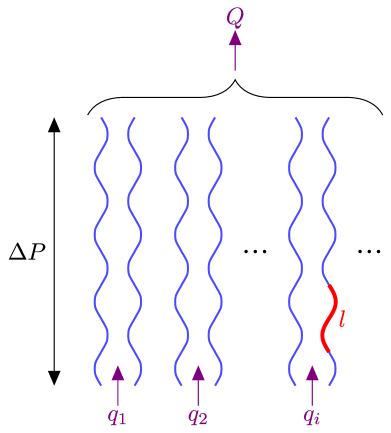
Figure 1: Capillary fiber bundle (CFB) model consists of a bundle of parallel sinusoidally shaped capillary tubes with period $l$. A global pressure drop $\Delta P$ drives the flow with volumetric flow rate $q_{i}$ in each tube $i$ which combine to produces a total volumetric flow rate $Q$.

As the main goal of this work is to examine the effect of mixed wettability, each one of the tubes in the CFB model has been given a wetting angle $\theta$ chosen randomly from a certain predefined distribution $\rho(\theta)$. This means that each tube has the same assigned wetting angle over its entire length. The flow is driven by applying a global pressure drop $\Delta P$ over the system. The total global volumetric flow rate $Q$ of the bundle of tubes is then calculated by considering the contributions to the flow given by each tube. This calculation has been carried out both analytically and numerically.

2.2 The Dynamic Pore Network Model Description

The second model that is used for the investigations in this work is a dynamic pore network (DPN) model, a complex numerical model which is not analytically solvable (sinha2019dynamic; amhb98; kah02; toh12; gvkh18). A sketch of the network used in the model is given in Fig. 2 and a short description will be given here. In this two-dimensional (2D) simulation, a porous network is modeled through a combination of links oriented with the same angle ($45^{\circ}$) from the flow direction and nodes connecting those links. The movement of the two immiscible fluids are modeled through tracking of their interfaces at each instant in time. The fluids get distributed to the neighboring links when they reach a node at the end of the link in which they have been traveling. The nodes themselves retain no volume. Embracing the concept of varying radius of the typical porous media, similar to what has been done in the CFB model, the links in this model is made to be hourglass shaped as shown with a zoomed in sketch in Fig. 2.

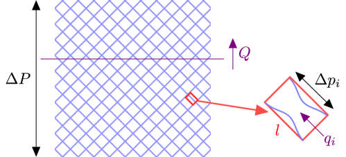
Figure 2: Two-dimensional dynamic pore network (DPN) model consists of hourglass shaped links with same length $l$ oriented with the same angle $(45^{\circ})$ from the flow direction. A global pressure drop $\Delta P$ drives the flow. The total volumetric flow rate $Q$ is constant over all the cross sections normal to the direction of the overall flow. Each link $i$ has a local flow rate $q_{i}$, length $l$ and a pressure drop $\Delta p_{i}$ over it.

The mixed wettability has been implemented into the DPN model by randomly choosing a wetting angle $\theta$ for each one of the links in the network from a certain predefined wetting angle distribution $\rho(\theta)$. As in the case with the first model, the flow in the DPN model is driven by a pressure drop $\Delta P$ over the system. When using periodic boundary conditions, $\Delta P$ is defined across a period of the system. The total volumetric flow rate $Q$ is constant over all the cross sections normal to the direction of the overall flow, as the one illustrated with a horizontal line in Fig. 2.

2.3 Commonalities

There are several commonalities in the two models. The smallest computational unit, which will be denoted SCU for ease of reference, in the CFB model is a single tube and that in the DPN model is a single link. Even though each SCU in the two models has uniform wettability, the entire system consisting of various such entities together describes a mixed wet porous media. In both models, the radius of each SCU $i$, with cylindrical symmetry around the center axis $\mathbf{x}$ has the form

$$r_{i}(x)=\frac{r_{0,i}}{1-a\cos\left(\frac{2\pi x}{l}\right)},$$ (2)

where $r_{0,i}$ is a constant and $a$ is the amplitude of the periodic variation. In the DPN model, $l$ in Eq. 2 is the length of the links, since the shape of the links covers only one period of oscillation, giving an hourglass form as shown in Fig. 2. In the CFB model, $l$ in Eq. 2 is the wavelength of the shape of the tubes, as shown in Fig. 1.

The flow within SCUs are governed by the following equations. In SCU $i$, the capillary pressure $p_{c,i}(x)$ across an interface between the two immiscible fluids with wetting angle $\theta_{i}$ can be derived from the Young-Laplace equation to be (blunt2017multiphase)

$$p_{c,i}(x)=\frac{2\sigma\cos{\theta_{i}}}{r_{i}(x)},$$ (3)

where $\sigma$ is the surface tension. For each SCU with length $l^{\prime}$ experiencing a pressure drop $\Delta p$ across its body, the fluid within it is forced to move due to the force exerted by the total effective pressure. Total effective pressure is the difference between $\Delta p$ and the total capillary pressure $\sum_{k}p_{c}(x_{k})$ due to all the interfaces with positions $x_{k}\in[0,l^{\prime}]$. Assuming that the radius does not deviate too much from its average value $\bar{r}_{i}$, the volumetric flow rate $q_{i}$ in SCU $i$ is given by (sinha2019dynamic; washburn1921dynamics)

$$q_{i}=-\frac{\pi\bar{r}_{i}^{4}}{8\mu_{i}l^{\prime}}\left(\Delta p_{i}-\sum_{k}p_{c,i}(x_{k})\right)$$ (4)

where $\mu_{i}$ is the saturation weighted viscosity of the fluids given by

$$\mu_{i}=s_{A,i}\mu_{A}+s_{B,i}\mu_{B}.$$ (5)

Here, $s_{A,i}=l^{\prime}_{A,i}/l^{\prime}$ and $s_{B,i}=l^{\prime}_{B,i}/l^{\prime}$ are saturations of the two fluids $A$ and $B$ with viscosities $\mu_{A}$ and $\mu_{B}$ and lengths $l^{\prime}_{A,i}$ and $l^{\prime}_{B,i}$. In the DPN model, $l^{\prime}$ is the same as $l$ from Eq. 2. In the CFB model, $l^{\prime}$ is the length of the whole tube. The capillary number $\mathit{Ca}$, which is the ratio of viscous to capillary forces, is related to $q_{i}$ through $\mathit{Ca}=\mu Q/(\sigma\alpha)$ where $Q$ is the sum of all $q_{i}$ through a cross sectional area $\alpha$ (sinha2019dynamic).

Note that due to the incompressible nature of the fluids examined in this work, $q$ given by Eq. 4 is the same for any position along a single SCU. Also note that all $\theta$ in this work are defined through fluid $A$, as shown in Fig. 3, which means the wetting angles of fluid $B$ are $180^{\circ}-\theta$. The fluid that makes the smallest angle with the solid wall is the wetting fluid in that region of the pore space and the other fluid is the non-wetting fluid.

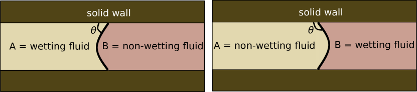
Figure 3: The wetting angles $\theta$ in this work are defined through fluid $A$. The fluid that makes the smallest angle with the solid wall is the wetting fluid while the other one is the non-wetting fluid.

3 Results

3.1 The Capillary Fiber Bundle Model Results

The analysis of flow in a single tube is presented in Subsec. 3.1.1. The theory is extended to a bundle of tubes with non-uniform wettability in Subsec. 3.1.2. The results from numerically solving the equations derived in Subsec. 3.1.2 give a holistic picture of the system. They are presented in LABEL:ssub:numerical_results and agree with the theoretical calculations from Subsec. 3.1.2. A further explanation of the results is given in LABEL:ssub:the_origin_of_beta.

3.1.1 A Single Tube

In the paper by sinha2013effective, they calculate the flow properties in a capillary tube with $\cos(\theta)=1$. Here, for a single tube, we will follow their calculations while keeping $\theta$ as a variable as it is needed for the rest of the work. The parameters $r_{0}$, $\mu$, $l$, $\sigma$, $a$, $l^{\prime}$ and $\Delta p$, as given in Eqs. 2, 3, 4 and 5, are kept constant for all the tubes. All the tubes have the same length $l^{\prime}=L$ and global applied pressure $\Delta p=\Delta P$.

We start by considering a capillary tube with $N$ bubbles. A “bubble” is one type of fluid restricted on two sides by the other fluid. Each bubble $j$ has the center of mass position $x_{j}$ and a width $\Delta x_{j}$. From Eqs. 2, 3, 4 and 5 we find that the volumetric flow rate through one tube is

$$q=-\frac{\pi\bar{r}^{4}}{8\mu L}\left[\Delta P+\sum_{j=0}^{N-1}\cos{\theta}\frac{4a\sigma}{r_{0}}\sin\left(\frac{\pi\Delta x_{j}}{l}\right)\sin\left(\frac{2\pi}{l}(x_{0}+\delta x_{j})\right)\right],$$ (6)

where $\delta x_{j}=x_{j}-x_{0}$. Due to the incompressible nature of the fluids, the velocity of the bubbles is approximately constant along the axis of flow and equal to $\mathop{}\!\mathrm{d}x_{0}/\mathop{}\!\mathrm{d}t\approx\mathop{}\!\mathrm{d}x_{j}/\mathop{}\!\mathrm{d}t\approx q/(\pi\bar{r}^{2})$. In addition, the effect of the variation in $\Delta x_{j}$ and $\delta x_{j}$ can be assumed to be small. With this, Eq. 6 can be rewritten as

$$\frac{\mathop{}\!\mathrm{d}x_{0}}{\mathop{}\!\mathrm{d}t}=-\frac{\bar{r}^{2}}{8\mu L}\left[\Delta P+\cos{\theta}\left(\Gamma_{s}\sin\left(\frac{2\pi x_{0}}{l}\right)+\Gamma_{c}\cos\left(\frac{2\pi x_{0}}{l}\right)\right)\right],$$ (7)

where

$$\Gamma_{s}=\sum_{j=0}^{N-1}\frac{4a\sigma}{r_{0}}\sin\left(\frac{\pi\Delta x_{j}}{l}\right)\cos\left(\frac{2\pi\delta x_{j}}{l}\right)$$ (8)

and

$$\Gamma_{c}=\sum_{j=0}^{N-1}\frac{4a\sigma}{r_{0}}\sin\left(\frac{\pi\Delta x_{j}}{l}\right)\sin\left(\frac{2\pi\delta x_{j}}{l}\right).$$ (9)

With algebraic manipulations, Eq. 7 can be rewritten as

$$\frac{\mathop{}\!\mathrm{d}x}{\mathop{}\!\mathrm{d}t}=-\frac{\bar{r}^{2}}{8\mu L}\left[\Delta P-\cos{\theta}\sqrt{\Gamma_{s}^{2}+\Gamma_{c}^{2}}\sin\left(\frac{2\pi x}{l}\right)\right],$$ (10)

where $x=x_{0}+[\arctan(\Gamma_{c}/\Gamma_{s})+\pi]l/2\pi$. Defining

$$\gamma=k_{\gamma}\cos\theta$$ (11)

with

$$k_{\gamma}=\sqrt{\Gamma_{s}^{2}+\Gamma_{c}^{2}},$$ (12)

write Eq. 10 as

$$\frac{\mathop{}\!\mathrm{d}x}{\mathop{}\!\mathrm{d}t}=-\frac{\bar{r}^{2}}{8\mu L}\left[\Delta P-\gamma\sin\left(\frac{2\pi x}{l}\right)\right].$$ (13)

We wish to calculate the average velocity of the bubbles as they travel from one end to the other end of a tube segment with length $l$ using a time $T$,

$$\left\langle\frac{\mathop{}\!\mathrm{d}x}{\mathop{}\!\mathrm{d}t}\right\rangle=\frac{l}{T}.$$ (14)

$T$ can be calculated by using the equation of motion in Eq. 13,

$$T =\int_{0}^{l}\left(\frac{\mathop{}\!\mathrm{d}x}{\mathop{}\!\mathrm{d}t}\right)^{-1}\mathop{}\!\mathrm{d}x$$

$$=-\frac{8\mu L}{\gamma\bar{r}^{2}}\int_{0}^{l}\frac{1}{\frac{\Delta P}{\gamma}-\sin\left(\frac{2\pi x}{l}\right)}\mathop{}\!\mathrm{d}x$$

$$=-\frac{8\mu Ll}{\bar{r}^{2}}\frac{\text{sgn}\left(\Delta P\right)}{\sqrt{\Delta P^{2}-\gamma^{2}}}.$$ (15)

Inserting the result in Eq. 15 into Eq. 14 and using the relation $\mathop{}\!\mathrm{d}x/\mathop{}\!\mathrm{d}t\approx q/(\pi\bar{r}^{2})$ gives the average volumetric flux equation

$$\langle q\rangle=-\frac{\pi\bar{r}^{4}}{8\mu L}\text{sgn}\left(\Delta P\right)\Theta(\left\lvert\Delta P\right\rvert-\left\lvert\gamma\right\rvert)\sqrt{\Delta P^{2}-\gamma^{2}},$$ (16)

where $\Theta$ is the Heaviside step function. From Eq. 16 we see that, on average, the direction of flow is opposite to the pressure drop, as expected. Additionally, we see that for a nonzero flow, $\Delta P$ needs to exceed a certain threshold $\gamma$ that is specific for the tube.

3.1.2 A Bundle of Tubes

In the CFB model, the global volumetric flow rate $Q$ of a bundle of tubes is the sum of the time-averaged individual volumetric flow rates $\langle q\rangle$ of all the tubes that carry flow. As remarked at the end of Subsec. 3.1.1, the tubes that carry flow are those that have a threshold $\gamma$ that satisfies the requirement $\left\lvert\Delta P\right\rvert>\left\lvert\gamma\right\rvert$. We will define a quantity $P_{t}$ which is the minimum possible $\gamma$ a tube can have. This means that the first active path across the entire system occurs once $\Delta P$ exceeds $P_{t}$. Let us also define $\gamma_{\text{max}}$ as the maximum possible $\gamma$ a tube can have, for later use. The factors that determine $\gamma$ can be seen from Eq. 11. Among those, $\theta$ is the only variable that varies from tube to tube, while the other quantities are set to be universal. Under a constant $\Delta P$, what determines which tubes in the bundle will conduct flow, while others do not is therefore their $\theta$. Using Eq. 11 and that $\theta\in[0^{\circ},180^{\circ}]$, the requirement for flow to happen in a tube can be rewritten as

$$\theta_{a}<\theta<\theta_{P_{t}}^{+}\quad\text{and}\quad\theta_{P_{t}}^{-}<\theta<\theta_{b},$$ (17)

with

$$\theta_{a}=\arccos\left(\text{min}\left(1,\frac{\left\lvert\Delta P\right\rvert}{k_{\gamma}}\right)\right),$$ (18)

$$\theta_{b}=\arccos\left(\text{max}\left(-1,-\frac{\left\lvert\Delta P\right\rvert}{k_{\gamma}}\right)\right)=180^{\circ}-\theta_{a},$$ (19)

$$\theta_{P_{t}}^{\pm}=\arccos\left(\pm\frac{\left\lvert P_{t}\right\rvert}{k_{\gamma}}\right).$$ (20)

Note that $\theta_{P_{t}}^{+}=\theta_{P_{t}}^{-}$ when $\left\lvert P_{t}\right\rvert=0$.

Since the flow requirement in Eq. 17 indicates the range of $\theta$ that give the system a nonzero flow, $Q$ can be expressed as a function of the probability distribution $\rho(\theta)$ of the wetting angles through

$$Q=\int_{\theta_{a}}^{\theta_{P_{t}}^{+}}\langle q\rangle\rho(\theta)\mathop{}\!\mathrm{d}\theta+\int_{\theta_{P_{t}}^{-}}^{\theta_{b}}\langle q\rangle\rho(\theta)\mathop{}\!\mathrm{d}\theta.$$ (21)

Inserting Eq. 16 into Eq. 21 gives

$$Q=-\frac{\pi\bar{r}^{4}\text{sgn}\left(\Delta P\right)}{8\mu L}\left[\int_{\theta_{a}}^{\theta_{P_{t}}^{+}}\sqrt{\Delta P^{2}-\gamma^{2}}\rho(\theta)\mathop{}\!\mathrm{d}\theta+\int_{\theta_{P_{t}}^{-}}^{\theta_{b}}\sqrt{\Delta P^{2}-\gamma^{2}}\rho(\theta)\mathop{}\!\mathrm{d}\theta\right].$$ (22)

Case studies with several different forms of $\rho(\theta)$ will be done numerically in LABEL:ssub:numerical_results. Here, we will solve Eq. 22 for a general $\rho(\theta)$ and show that the exponent $\beta$ in

$$Q\propto\left(\left\lvert\Delta P\right\rvert-\left\lvert P_{t}\right\rvert\right)^{\beta}$$ (23)

is

$$\beta=\begin{cases}1,&\text{ for }\left\lvert\Delta P\right\rvert-\left\lvert P_{t}\right\rvert\gg\left\lvert\gamma_{\text{max}}\right\rvert\qquad\qquad\,(\text{\lx@cref{creftype~refnum}{cs:beta1}}),\\ 2,&\text{ for }\left\lvert P_{t}\right\rvert\ll\left\lvert\Delta P\right\rvert-\left\lvert P_{t}\right\rvert\ll\left\lvert\gamma_{\text{max}}\right\rvert\quad(\text{\lx@cref{creftype~refnum}{cs:beta2}}),\\ 1.5,&\text{ for }\left\lvert\Delta P\right\rvert-\left\lvert P_{t}\right\rvert\ll\left\lvert P_{t}\right\rvert\qquad\qquad\quad\>(\text{\lx@cref{creftype~refnum}{cs:beta1pt5}}).\end{cases}$$ (24)

Here, $\left\lvert\gamma_{\text{max}}\right\rvert$ is the maximum possible threshold pressure a tube can have.

Case 1

:   $\left\lvert\Delta P\right\rvert-\left\lvert P_{t}\right\rvert\gg\left\lvert\gamma_{\text{max}}\right\rvert$

Using that $\left\lvert\Delta P\right\rvert$ is large in this case, we can write

$$\sqrt{\Delta P^{2}-\gamma^{2}}\approx\left\lvert\Delta P\right\rvert.$$ (25)

Inserting Eq. 25 into Eq. 22 and using that the distribution $\rho(\theta)$ is normalized to $1$, gives

$$Q\approx-\frac{\pi\bar{r}^{4}\text{sgn}\left(\Delta P\right)}{8\mu L}\left\lvert\Delta P\right\rvert\approx-\frac{\pi\bar{r}^{4}\text{sgn}\left(\Delta P\right)}{8\mu L}\left(\left\lvert\Delta P\right\rvert-\left\lvert P_{t}\right\rvert\right).$$ (26)

In the last step, we have used that $\left\lvert P_{t}\right\rvert$ which is the minimum $\left\lvert\Delta P\right\rvert$ needed to achieve $Q>0$, is a much smaller number than $\left\lvert\Delta P\right\rvert$. For the equations derived for all three cases in Eq. 24, we wish to express $Q$ in terms of $\left\lvert\Delta P\right\rvert-\left\lvert P_{t}\right\rvert$ for ease of comparison with Eq. 23. Comparing Eq. 26 with Eq. 23, one gets $\beta=1$ for case 1.

Common for Case 2 and Case 3:

Eq. 24 states that the effective pressure obeys $\left\lvert\Delta P\right\rvert-\left\lvert P_{t}\right\rvert\ll\left\lvert\gamma_{\text{max}}\right\rvert$ in case 2, while it obeys $\left\lvert\Delta P\right\rvert-\left\lvert P_{t}\right\rvert\ll\left\lvert P_{t}\right\rvert$ in case 3. From Eq. 11, the threshold pressure $\gamma$ is so that $\left\lvert\gamma\right\rvert\leq k_{\gamma}$. This criterion should also be followed by the maximum possible $\left\lvert\gamma\right\rvert$ which is $\left\lvert\gamma_{\text{max}}\right\rvert$ and the minimum possible $\left\lvert\gamma\right\rvert$ which is $\left\lvert P_{t}\right\rvert$. Combining these information, a common requirement for cases 2 and 3 should be

$$\left\lvert\Delta P\right\rvert-\left\lvert P_{t}\right\rvert\ll k_{\gamma}.$$ (27)

Eq. 18 then becomes

$$\theta_{a} =\arccos\left(\frac{\left\lvert\Delta P\right\rvert}{k_{\gamma}}\right),$$

$$=\arccos\left(\frac{\left\lvert\Delta P\right\rvert-\left\lvert P_{t}\right\rvert+\left\lvert P_{t}\right\rvert}{k_{\gamma}}\right),$$

$$\approx\arccos\left(\frac{\left\lvert P_{t}\right\rvert}{k_{\gamma}}\right)-\frac{\left\lvert\Delta P\right\rvert-\left\lvert P_{t}\right\rvert}{\sqrt{k_{\gamma}^{2}-{P_{t}^{2}}}}.$$ (28)

where Eq. 27 was used in the last step.

Next, based on Eq. 27, Taylor expanding the integrands of Eq. 22 with respect to $\theta$ around $\theta^{\pm}_{P_{t}}$ gives

$$Q\approx -\frac{\pi\bar{r}^{4}\text{sgn}\left(\Delta P\right)}{8\mu L}\left[\int_{\theta_{a}}^{\theta_{P_{t}}^{+}}\sqrt{\Delta P^{2}-P_{t}^{2}}\ \rho\left(\theta_{P_{t}}^{+}\right)\mathop{}\!\mathrm{d}\theta\right]$$

$$-\frac{\pi\bar{r}^{4}\text{sgn}\left(\Delta P\right)}{8\mu L}\left[\int_{\theta_{P_{t}}^{-}}^{\theta_{b}}\sqrt{\Delta P^{2}-P_{t}^{2}}\ \rho\left(\theta_{P_{t}}^{-}\right)\mathop{}\!\mathrm{d}\theta\right].$$ (29)

Performing this integrations using the integration limits given in Eqs. 28 and 20 and that $\theta_{b}=180^{\circ}-\theta_{a}$ (Eq. 19) gives

$$Q\approx- \left[\frac{\pi\bar{r}^{4}\text{sgn}\left(\Delta P\right)}{8\mu L}\frac{\rho\left(\theta_{P_{t}}^{+}\right)+\rho\left(\theta_{P_{t}}^{-}\right)}{\sqrt{k_{\gamma}^{2}-P_{t}^{2}}}\right]$$

$$\times\left(\left\lvert\Delta P\right\rvert-\left\lvert P_{t}\right\rvert\right)^{3/2}\left(\left(\left\lvert\Delta P\right\rvert-\left\lvert P_{t}\right\rvert\right)+2\left\lvert P_{t}\right\rvert\right)^{1/2}.$$ (30)

Eq. 30 holds true for both LABEL:cs:beta2 and LABEL:cs:beta1pt5.