Paccagnan and Gairing

In Congestion Games, Taxes Achieve Optimal Approximation

In Congestion Games,
Taxes Achieve Optimal Approximation

Dario Paccagnan Department of Computing, Imperial College London, London, UK, d.paccagnan@imperial.ac.uk Martin Gairing Department of Computer Science, University of Liverpool, Liverpool, UK, m.gairing@liverpool.ac.uk

In this work, we consider the problem of minimising the social cost in atomic congestion games. For this problem, we provide tight computational lower bounds along with taxation mechanisms yielding polynomial time algorithms with optimal approximation.

Perhaps surprisingly, our results show that indirect interventions, in the form of efficiently computed taxation mechanisms, yield the same performance achievable by the best polynomial time algorithm, even when the latter has full control over the agents’ actions. It follows that no other tractable approach geared at incentivizing desirable system behavior can improve upon this result, regardless of whether it is based on taxations, coordination mechanisms, information provision, or any other principle. In short: Judiciously chosen taxes achieve optimal approximation. Three technical contributions underpin this conclusion. First, we show that computing the minimum social cost is NP-hard to approximate within a given factor depending solely on the admissible resource costs. Second, we design a tractable taxation mechanism whose efficiency (price of anarchy) matches this hardness factor, and thus is worst-case optimal. As these results extend to coarse correlated equilibria, any no-regret algorithm inherits the same performances, allowing us to devise polynomial time algorithms with optimal approximation.

congestion games, minimum social cost, hardness of approximation, optimal mechanism, polynomial time algorithms with optimal approximation, taxation mechanism, price of anarchy.

1 Introduction

Decision-making in the presence of congestion effects is a central topic in the operations research and game theory literature. Within this arena, the celebrated congestion game model proposed by rosenthal1973class offers a fundamental framework to study resource allocation problems prone to congestion, finding fitting applications in transportation, telecommunications, scheduling, and many other disciplines.

In an atomic congestion game, we are given a finite set of resources and a finite number of agents. Every agent is endowed with a set of feasible allocations, each corresponding to a subset of the set of resources. These subsets may, for example, correspond to machines where an agent wishes to schedule their jobs, or to paths connecting a given origin-destination in a graph. When selecting an allocation, each agent incurs an additive cost over the chosen resources, where the cost of a particular resource depends solely on the number of agents using it, i.e., on the congestion on that resource. At the system level, the quality of a joint allocation is measured through the social cost by summing all the agents costs.

Perhaps the most commonly encountered class of congestion games is that of network congestion games, where each feasible allocation corresponds to a path connecting a given pair of origin-destination nodes over a shared graph. This class of congestion games arises in the study of classical optimization problems in road-traffic, wireless-network, and minimum-power routing – see (rosenthal1973class, tekin2012atomic, AndrewsAZZ12) respectively. However, congestion games find interesting applications also beyond network-like settings for example in machine scheduling (suri2007selfish), distributed control (marden2013distributed), sensor allocation (paccagnan2018distributed), and factory production (rosenthal1973class).

In this work we are concerned with a system optimal perspective on congestion games, complementary to much of the existing literature. Specifically, we study the problem of minimising the social cost. We do so in two stages, depending on whether agents are modelled as strategic decision-makers or not.

We start by considering the case where agents are non-strategic, i.e., the case where we can directly control their allocations for the purpose of minimizing the social cost. This point of view stems from the observation that, in many circumstances, the planner is interested in a globally optimal solution to a congestion game where agents can be easily coordinated. Such problems arise commonly, e.g., in load balancing (awerbuch1995load), power routing (AndrewsAZZ12), or fleet management in mobility on-demand where a central operator is responsible for routing an entire fleet of cars (zardini2021analysis). However, in spite of the significant scientific interest, the fundamental nature of this model, and its ties to many related questions in operations research, little is known regarding the problem of minimizing the social cost in congestion games. Most notably, it remains unclear what solution quality can be achieved by efficient (i.e. polynomial time) algorithms, and what are the inherent computational barriers to achieving such goal. Specifically, no tight hardness of approximation is known to date, nor a polynomial time algorithm with optimal approximation is available. Our manuscript completely settles these questions in a series of three contributions.

Our first contribution shows that minimizing the social cost in congestion games is NP-hard to approximate within an explicitly given factor depending solely on the class of resource costs. Prior to our work, no tight computational lower bound was known, even for the special case of linear resource costs. Our second and third contributions provide polynomial time algorithms with an approximation factor matching such hardness barrier. Taken together, these results certify that the algorithms we propose are optimal in the sense that they yield the best possible polynomial time approximation with respect to the worst-case instance. As such, they leave open the possibility that a different class of algorithms might provide a better performance on an instance-by-instance case. However, we will see that the approximation we derive is near-optimal for many commonly encountered real-world settings, including the case where resource costs increase not too steeply (e.g., polynomials of low degree, logarithms), or where the uncongested and congested costs are of comparable magnitude (e.g., BPR functions). As the proposed approach applies even when agents are strategic, we now present such contributions within this more challenging setting.

Decision-making in the presence of strategic agents dates back to the seminal works of morgenstern1953theory and nash1950equilibrium, which laid the foundation for the nascent field of game theory. Most notably, their work contributed to establishing the notion of equilibrium, e.g., Nash equilibrium, which describes the outcome arising from the interaction of strategic decision-makers aiming to minimimize their individual cost functions. Building over this initial work, researchers soon realized that equilibrium allocations often display a significant performance degradation when compared to the corresponding optimal solutions, leading to the definition of the so-called price of anarchy, commonly used to quantify the worst-case equilibrium efficiency (koutsoupias1999worst). A prototypical example of this issue is provided by road-traffic routing: When drivers choose routes that minimize their own travel time, the aggregate congestion could be much higher compared to that of a centrally-imposed routing. While improved performances could be attained if a coordinator was able to dictate the choices of each agent, imposing such control is often infeasible or impossible in these settings, with traffic routing providing just one illustration. Hence, different approaches including coordination mechanisms (ChristodoulouKN09), Stackelberg strategies (BonifaciHS10), taxation mechanisms (caragiannis2010taxes), information provision (BhaskarCKS16), and alternative methods for sharing resource costs (GkatzelisKR16) have been proposed as indirect interventions to influence the resulting equilibrium efficiency. Amongst these, taxation mechanisms, where agents pay an additional cost for utilizing a resource, have attracted significant attention, as witnessed by the growing literature on the topic, see (harks2019pricing) and references therein. Yet, the problem of designing taxation mechanisms optimizing the equilibrium efficiency remains largely open, even for classical settings such as that of atomic congestion games (harks2019pricing). Additionally, it remains unclear, if, and to what extent, the use of indirect interventions reduces the best achievable performance, thus prompting a natural question: Is there any performance degradation incurred when moving from centrally imposed decision-making to the use of indirect interventions, such as taxation mechanisms?

Perhaps surprisingly, our work answers this question in the negative, showing that no performance degradation arises when taxation mechanisms are judiciously designed. Specifically, our second contribution derives polynomially-computable taxation mechanisms ensuring that any corresponding equilibrium outcome has an efficiency (price of anarchy) matching the hardness factor derived in this paper, that is, the same performance achievable by the best centralized polynomial time algorithm. Before this work, optimal taxation mechanisms have been unavailable.

While this result holds for the commonly employed notion of pure Nash equilibrium, it also extends to more general notions of equilibrium that can be computed more efficiently (e.g., correlated and coarse correlated equilibria). Moreover, it extends to no-regret online learning algorithms where agents update their allocations and achieve low regret, in the same spirit of the “total price of anarchy” pioneered by BlumHLR08. Our third and final contribution builds upon this observation to derive polynomial time algorithms achieving the optimal approximation factor. When taken together, the upshot of our work can be summarized as follows: [leftmargin=1.35cm] In congestion games, judiciously designed taxes achieve optimal approximation, and no other tractable intervention, whether based on coordination mechanisms, information provision, or any other principle can improve upon this result.

Significance and comparison with existing results

Our work connects with a number of existing results, in addition to closing different open questions, as we briefly highlight next. We refer to Section 1.3 for a more detailed literature review, including a discussion on the continuous flow counterpart of congestion games (nonatomic model).

The problem of determining computational lower bounds for minimizing the social cost in atomic congestion games has been initially studied by MeyersS12. Since then, a number of works have pursued a similar line of research, though no tight bounds were known. Our work provides the best possible inapproximability results, completely settling the hardness question for congestion games with general underlying resource costs.

The study of taxation mechanisms has recently received growing attention, especially within the congestion games literature. Nevertheless, prior to this work, a methodology to design optimal taxation mechanisms (i.e., mechanisms minimizing the price of anarchy) was not known. For congestion games with polynomial costs, caragiannis2010taxes (for linear) and BiloV19 (for polynomial) propose taxes whose efficiency can be quantified a priori. Both papers conjecture that their design is optimal. Our work resolves the problem of determining optimal taxes for the broader class of congestion games with non-decreasing and semi-convex resource costs, proving these conjectures as a special case. Rough_barrier studies how lower bounds on the price of anarchy can be derived from computational lower bounds. For congestion games with optimal taxes, we show that such an approach does provide tight bounds.

The best known approximation algorithm for minimizing the social cost in congestion games is due to Makarychev18, and leverages a natural linear programming relaxation jointly with a randomized rounding scheme. While their result applies to the more general class of optimization problems with a “diseconomy of scale”, the algorithms we propose here enjoy an equal or strictly better approximation ratio, and can not be further improved, owing to the matching hardness result provided.

1.1 Congestion game model and taxation mechanisms

In a congestion game we are given a set of agents $\{1,\dots,N\}$, and a set of resources $\mathcal{R}$. Each agent can choose a subset of the set of resources which she intends to use. We list all feasible choices for agent $i$ in the set $\mathcal{A}_{i}\subseteq 2^{\mathcal{R}}$. The cost for using each resource $r\in\mathcal{R}$ depends only on the total number of agents concurrently selecting that resource, and is denoted with $\ell_{r}:\mathbb{N}\rightarrow\mathbb{R}_{>0}$. Once all agents have made a choice $a_{i}\in\mathcal{A}_{i}$, each agent incurs a cost obtained by summing the costs of all resources she selected. Finally, the social cost represents the sum of the resource costs incurred by all agents

$${\rm{SC}}(a)=\sum_{i=1}^{N}\sum_{r\in a_{i}}\ell_{r}(|a|_{r}),$$ (1)

where $|a|_{r}$ denotes the number of agents selecting resource $r$ in allocation $a=(a_{1},\dots,a_{n})$. Given an instance $G$ of a congestion game, we denote with MinSC the problem of globally minimizing the social cost in (1).

Taxation mechanisms.

As self-interested decision making often deteriorates the system performance, taxation mechanisms have been proposed to ameliorate this issue. Formally, a taxation mechanism $T:G\times r\rightarrow\tau_{r}$ associates an instance $G$, and a resource $r\in\mathcal{R}$ to a taxation function $\tau_{r}:\mathbb{N}\rightarrow\mathbb{R}_{\geq 0}$. Note that each taxation function $\tau_{r}$ is congestion-dependent, that is, it associates the number of agents in resource $r$ to the corresponding tax. As a consequence, each agent $i$ experiences a cost factoring both the cost associated to the chosen resources, and the tax, i.e., C_i(a)=∑_r∈a_i [ℓ_r(—a—_r)+τ_r(—a—_r)]. As typical in the literature, we measure the performance of a given taxation mechanism $T$ using the ratio between the social cost incurred at the worst-performing outcome, and the minimum social cost. Given the self-interested nature of the agents, an outcome is commonly described by any of the following classical equilibrium notions: pure or mixed Nash equilibria, correlated or coarse correlated equilibria. When considering pure Nash equilibria, for example, the performance of a taxation mechanism $T$ over the class of congestion games $\mathcal{G}$ is gauged using the notion of price of anarchy originally introduced by koutsoupias1999worst, i.e.,

$$\mathrm{PoA}(T)=\sup_{G\in\mathcal{G}}\frac{{\tt{NeCost}}(G,T)}{{\tt{MinCost}}(G)},$$ (2)

where ${\tt{MinCost}}(G)=\min_{a\in\mathcal{A}}SC(a)$ is the minimum social cost for instance $G$, and ${\tt{NeCost}}(G,T)$ denotes the highest social cost at a Nash equilibrium obtained when employing the mechanism $T$ on the game $G$. By definition, $\mathrm{PoA}(T)\geq 1$ and the lower the price of anarchy, the better performance $T$ guarantees. While it is possible to define the notion of price of anarchy for each and every equilibrium class mentioned, we do not pursue this direction, as we will show that all these metrics coincide within our setting. Thus, we will simply use $\mathrm{PoA}(T)$ to refer to the efficiency values of any and all these equilibrium classes. Finally, we observe that, while taxation mechanisms influence the agents’ perceived cost, they do not impact the expression of the social cost, which is still of the form in (1).

All our results hold for the widely studied case of non-decreasing semi-convex resource costs, corresponding to all resource costs satisfying the following assumption.

The function $\ell:\mathbb{N}\rightarrow\mathbb{R}_{>0}$ is non-decreasing and semi-convex.

Notation.

In our work $\mathbb{N}$, $\mathbb{N}_{0}$, $\mathbb{R}$, $\mathbb{R}_{\geq 0}$, $\mathbb{R}_{>0}$ denote the sets of natural numbers, natural numbers including zero, real numbers, non-negative real numbers, and positive real numbers. Further, $\text{Poi}(x)$ denotes a Poisson distribution with parameter $x\in\mathbb{R}_{>0}$. In the remainder of the manuscript, we extend the domain of definition of all resource costs from $\mathbb{N}$ to $\mathbb{N}_{0}$ by setting their value to zero. This is without loss of generality. Indeed, the value of $\ell_{r}(0)$, does not play any role with respect to all quantities we have introduced thus far, e.g., the social cost in (1), since $\ell_{r}(|a|_{r})$ is always evaluated for $|a|_{r}\geq 1$. However, doing so will allow us to simplify notation.

1.2 Our contributions

The resounding message contained in this work can be summarized as follows: In congestion games, optimally designed taxation mechanisms can be tractably computed, and achieve the same performance of the best centralized polynomial time algorithm. Further, such approximation is near-optimal in a variety of commonly-encountered settings. Three technical contributions substantiate this claim, and are further discussed in the ensuing paragraphs:

• We prove a tight NP-hardness result for minimizing the social cost.

• We design a tractable taxation mechanism whose price of anarchy matches the hardness factor.

• We obtain a polynomial time algorithm with the best possible approximation ratio for the social cost. We do so combining the previous results with existing algorithms (e.g., no-regret dynamics).

Results ii) and iii) extend to network congestion games, as we discuss in the conclusions.

Inapproximability of minimum social cost. Our first contribution is concerned with determining tight inapproximability results for the problem of minimizing social cost in congestion games. Our hardness result applies already in the setup where all resources feature the same cost.

Theorem 1.1

Let $\ell:\mathbb{N}\rightarrow\mathbb{R}_{>0}$ satisfing Assumption 1.1 be given. In congestion games where all resources feature the same cost $\ell$, MinSC is NP-hard to approximate within any factor smaller than ρ_ℓ=sup_x∈NEP∼Poi(x)[Pℓ(P)]xℓ(x), where we define $\ell(0)=0$. If $\rho_{\ell}=\infty$, then MinSC is NP-hard to approximate within any finite factor.

Naturally, Theorem 1.1 applies directly to richer classes of congestion games, whereby resource costs can differ. For example, if resource costs belong to a set of functions $\mathscr{L}$, then MinSC is NP-hard to approximate within any factor smaller than that produced by the worst function in $\mathscr{L}$, i.e., $\sup_{\ell\in\mathscr{L}}\rho_{\ell}$. As a special case, we obtain hardness results for the thoroughly studied class of polynomial congestion games with maximum degree $d$. In this case, the highest degree monomial $x^{d}$ determines the worst factor (see Section 2.4), which reduces to the $(d+1)$’st Bell number, as summarized in the following statement.

Corollary 1.2

In congestion games with resource costs obtained by non-negative combinations of $1$, $\dots$, $x^{d}$, MinSC is NP-hard to approximate within a factor smaller than the $\!(d\!+\!1)\!$’st Bell number.

We note that Bell numbers grow as function of the degree $d$, so that the corresponding inapproximability factor also grows with $d$. However, for many problems of interest, resource costs feature further properties that can be exploited to reduce such factor. This is interesting, since the algorithms we propose will provide approximations matching this factor. For example, in road-traffic routing, the commonly employed BPR functions take the form $\ell_{r}(x)=\alpha_{r}x^{4}+\beta_{r}$ where $\alpha_{r}\ll\beta_{r}$ for all resources, see for example the commonly employed Sioux Fall network and other instances from (TransNet). In this context, a direct application of Theorem 1.1 provides inapproximability factors significantly closer to one. We elucidate this point in the following corollary where we look at congestion games with affine resource costs, as this allows to present a concise analytical result. However, a similar result holds for BPR functions, as demonstrated in Figure 1 (left).

Corollary 1.3

In congestion games with affine resource costs of the form $\ell_{r}(x)=\alpha_{r}x+\beta_{r}$, where $\max_{r}{\alpha_{r}}/({\alpha_{r}+\beta_{r}})\leq q$, MinSC is NP-hard to approximate within a factor smaller than $1+q$.

Figure 1: Inapproximability factors for congestion games with BPR resource costs $\ell_{r}(x)=\alpha_{r}x^{4}+\beta_{r}$ (left) and affine resource costs $\ell_{r}(x)=\alpha_{r}x+\beta_{r}$ (right), parametrized by $\max_{r}\alpha_{r}/\beta_{r}$. Commonly encountered instances, e.g., those taken from (TransNet) feature $\alpha_{r}\ll\beta_{r}$ yielding an inapproximability factor close to one, see markers on the left panel.

The latter result shows that the inapproximability factor depends only on the ratios between the coefficients $\alpha_{r}$ and $\beta_{r}$. To see this, denote $\max_{r}{\alpha_{r}}/{\beta_{r}}=\kappa$, and observe that $\max_{r}{\alpha_{r}}/({\alpha_{r}+\beta_{r}})={\kappa}/({\kappa+1})$ when $\beta_{r}\neq 0$. Consequently, the inapproximability factor $1+q$ can be rewritten more conveniently as $1+{\kappa}/({\kappa+1})$, see Fig. 1 (right) for a plot. In the regime where $\alpha_{r}\ll\beta_{r}$ for all resources, we have $\kappa\ll 1$, so that the inapproximability factor is close to one. When this ratio grows, the corresponding factor also grows up until it reaches its maximum when $\beta_{r}\rightarrow 0$ for some resource. In other words, the inapproximability factor depends on the ratio between the speed at which congestion translates into cost (here $\alpha_{r}$) and the uncongested cost (here $\beta_{r}$). Interestingly, in many setting the ratio ${\alpha_{r}}/{\beta_{r}}\ll 1$ , thus ensuring that the forthcoming algorithms will provide near-optimal approximation.

Regarding our techniques, the computational lower bounds are shown by reducing the problem of minimizing the social cost in congestion games from the gap label cover problem implicitly defined in Feige98. A central tool we leverage in our reduction is a gadget called partitioning system, generalizing that in Feige98. The challenge in defining this object stems from the fact that, in congestion games, the cost experienced over each resource depends on the actual number of agents selecting that resource, contrary to Feige98 where the welfare accrued depends solely on whether that resource is selected or not. The expression of the hardness factor (1.1) falls from the very definition of such object, which must be duplicated multiple times and carefully arranged in our construction to ensure hardness of the underlying instance. Conceptually, partitioning systems are constructed so that, in our reduction, agents have two types of allocations: either they coordinate themselves on an allocation with low social cost, or they opt for an allocation with high social cost. The inapproximability factor in (1.1) is precisely the ratio between these “high” and “low” social costs, see Section 2.1.2. Partitioning systems have been recently applied also by DudyczMMS20 and barman2021tight in the context of approval voting, and for a generalization of the maximum coverage problem. To the best of our knowledge, our work is the first that employs such gadgets to prove hardness of cost minimization problems.

Taxes achieve optimal approximation. Our second contribution provides a technique to efficiently design taxation mechanisms whose efficiency (price of anarchy) matches the hardness result. The following statement is a succinct variant of that in Theorem 3.3 where we also give an expression for the taxation mechanism.

Theorem 1.4

Consider the class of congestion games where each resource cost belongs to a set of functions $\mathscr{L}$ satisfying Assumption 1.1. Then, for any given $\varepsilon>0$, it is possible to efficiently compute a taxation mechanism whose price of anarchy is upper bounded by $\sup_{\ell\in\mathscr{L}}\rho_{\ell}+\varepsilon$. The result holds for pure/mixed Nash and correlated/coarse correlated equilibria.

The extension to coarse correlated equilibria is significant as it gives performance bounds that apply not only to Nash equilibria, but also whenever agents revise their action and achieve low regret. This imposes much weaker assumptions on both the game and its participants’ behaviour (roughgarden2015intrinsic). Whilst the theorem applies to a broad class of resource costs, when specialized to polynomial congestion games of degree $d$, it allows to efficiently design taxation mechanisms whose price of anarchy equals the $(d+1)$’st Bell number plus $\varepsilon$, for any arbitrarily small choice of $\varepsilon>0$.

We derive taxes whose efficiency matches the hardness factor leveraging two chief ingredients: a parametrized class of taxation mechanisms satisfying a key recursion, and a suitably defined convex optimization program. The convex optimization problem we consider corresponds to a modification of the original MinSC, whereby we relax the integrality constraints and replace the cost $x\ell_{r}(x)$ produced by each resource with $\mathbb{E}_{P\sim\text{Poi}(x)}[P\ell_{r}(P)]$, see (3). The solution vector of this program (which is provably convex) is used as set of parameters for the class of mechanisms previously defined. The performance bound on the price of anarchy is finally shown through a smoothness-like approach, where we leverage both the expression of the mechanisms and the solution vector of the convex program.

Tight polynomial algorithms. Since the result in Theorem 1.4 holds also for correlated/coarse correlated equilibria, we can leverage existing polynomial time algorithms to compute such equilibria, and inherit an approximation ratio matching the corresponding price of anarchy. The following statement summarizes this result, while the ensuing discussion provides two possible approaches to do so. We remark that Corollary 1.5 is a direct consequence of Theorem 1.4 and polynomial computability of correlated equilibria (JiangL15). The fact that the resulting approximation factor we obtain always matches or strictly improves upon that of Makarychev18 is shown in LABEL:subsec:comparison-sviri.

Corollary 1.5

Consider congestion games where each resource cost belongs to a set of functions $\mathscr{L}$ satisfying Assumption 1.1. Then, for any $\varepsilon>0$, there exists a polynomial time algorithm computing an allocation with cost lower than $(\sup_{\ell\in\mathscr{L}}\rho_{\ell}+\varepsilon)\cdot\min_{a\in\mathcal{A}}{\rm{SC}}(a)$.

The approximation ratio presented in Corollary 1.5 can be achieved, for example, as follows. Given a desired tolerance $\varepsilon>0$, we design a taxation mechanisms ensuring a price of anarchy of $\sup_{\ell\in\mathscr{L}}\rho_{\ell}+\varepsilon/2$, which can be done in polynomial time thanks to Theorem 1.4. We use such taxation mechanisms, and compute an exact correlated equilibrium in polynomial time leveraging the result of JiangL15, who propose a variation of the Ellipsoid Against Hope algorithm from papadimitriou2008computing. Remarkably, JiangL15 guarantees that the resulting correlated equilibrium has polynomial-size support, i.e., it places non-zero probability only over a polynomial number of pure strategy profiles. Hence, we compute a correlated equilibrium and enumerate all pure strategy profiles in its support, identifying with $a^{*}$ that with lowest cost. Since the price of anarchy bounds of Theorem 1.4 hold for correlated equilibria, the pure strategy profile $a^{*}$ inherits a matching (or better) approximation ratio.

Alternatively, one can employ the same taxation mechanism as in the above, and let agents simultaneously revise their action for $t$ rounds employing a no-regret algorithm. Well-known families of such algorithms include Multiplicative-Weights, and Follow the Perturbed/Regularized Leader whereby the average regret decays to an arbitrary $\varepsilon$ in a polynomial number of rounds, see cesa2006prediction, KalaiV05. We keep track of the pure strategy profile $a^{*}_{t}$ with the lowest social cost encountered during the $t$ rounds of any such algorithm t. Owing to (roughgarden2015intrinsic, Thm 3.3), its approximation ratio is upper bounded by the corresponding price of anarchy plus an error term that goes to zero with the same rate of the average regret. Waiting for polynomially many rounds suffices to reduce the error as desired.

1.3 Related work

As our work provides tight computational lower bounds, optimal taxation mechanisms, and polynomial time algorithms with the best possible approximation, we review the relevant literature connected with these three areas in the ensuing paragraphs. We conclude comparing our results with those available for the continuous flow counterpart of congestion games (nonatomic model).

Computational lower bounds.

The study of computational lower bounds for minimizing the social cost in congestion games has been pioneered by MeyersS12, though remarkable precursors include ChakrabartyMN05, as well as BlumrosenD06 who considered a notably different model whereby agent-specific cost functions are utilized. Relative to the classical model of congestion games with convex non-decreasing resource costs, Meyers and Schulz show that minimizing the social cost is strongly NP-hard, and it is hard to approximate within any finite factor, unless P=NP. Identical results are shown for network congestion games. Whilst this might feel as a contradiction of our results, it is worth noting that their analysis allows for resource costs to be adversarily selected amongst any convex non-decreasing function. On the contrary, our result can be thought of as a refined version of theirs, whereby the computational lower bound we derive is parametrized by the class of admissible resource costs. Naturally, we recover their inapproximability result when resource costs can be arbitrarily selected amongst convex non-decreasing functions.

Motivated by the possibility to translate computational lower bounds to lower bounds on the price of anarchy, Rough_barrier also studied this problem. Relative to polynomial resource costs of maximum degree $d$ and non-negative coefficients, he showed that minimizing the social cost is inapproximable within any factor smaller than $(\beta d)^{d/2}$, for some constant $\beta>0$. In this setting, even without taxes, equilibria with much better performance are guaranteed to exist. In particular, the price of stability (measuring the quality of the best-performing equilibrium) is known to grow only linearly with the degree $d$ (CG16). While coordinating the agents to one such good equilibrium is highly desirable, our hardness result implies that this cannot be achieved in polynomial time.

Spurred by the inapproximability results of MeyersS12, and Rough_barrier, a number of works have focused on restricting the allowable class of problems: PiaFM17 study totally unimodular congestion games and show NP-hardness for the asymmetric case; Castiglioni2020signaling show NP-hardness even in singleton congestion games with affine resource costs. Similar questions have been explored for online versions of the problem by KlimmST19.

Taxation mechanisms.

Different approaches, such as coordination mechanisms (ChristodoulouKN09), Stackelberg strategies (Fotakis10a), taxation mechanisms (caragiannis2010taxes), signalling (BhaskarCKS16), cost-sharing strategies (GairingKK20), and many more, have been proposed to cope with the performance degradation associated to selfish decision making. Amongst them, taxation mechanism have attracted significant attention thanks to their ability to indirectly influence the resulting system performance. While the study of taxation mechanisms in road-traffic networks was initiated by pigou, who utilized a continuous flow model (nonatomic congestion games), the design of taxation mechanisms in (atomic) congestion games was pioneered much more recently by caragiannis2010taxes. In this respect, caragiannis2010taxes and many of the subsequent works, build on the solid theoretical ground developed in the years subsequent to the definition of the price of anarchy (koutsoupias1999worst), including exact knowledge of the price of anarchy in congestion games with linear (christodoulou2005price, awerbuch2005price) and polynomial (aland2006exact) resource costs, the advent of the smoothness framework (roughgarden2015intrinsic), as well as primal dual approaches (bilo2018unifying, chandan19optimaljournal).

While these results provide us with a strong theory to quantify the price of anarchy, prior to this work, the design of optimal taxation mechanisms (i.e., taxation mechanisms minimizing the price of anarchy) has been an open question even when restricting attention to linear resource costs. Most notably, caragiannis2010taxes considers linear congestion games and designs taxation mechanisms achieving a price of anarchy of $2$ for mixed Nash equilibria. More recently, BiloV19 extend their results to polynomial congestion games of degree $d$ achieving a price of anarchy (for coarse correlated equilibria) equal to the $(d+1)$’st Bell number. Our work resolves the problem of designing optimal taxation mechanisms for more general congestion games with semi-convex non-decreasing resource costs, and, as a special case, shows that the mechanisms proposed for linear (caragiannis2010taxes) and polynomial (BiloV19) resource costs are optimal, as conjectured by the authors.

Perhaps closest in spirit to our work, is the recent result by paccagnan2019incentivizing, whereby the authors leverage a tractable linear programming formulation to design optimal taxation mechanisms that utilize solely local information. Naturally, the corresponding values of the optimal price of anarchy they achieve are inferior to ours (here, we design optimal taxation mechanisms without any restrictions on what type of information we use), though the efficiency values derived therein are remarkably close to the optimal values obtained here. For example, for affine (resp. quadratic) congestion games, they achieve an optimal price of anarchy of 2.012 (resp. 5.101), to be compared with a value of 2 (resp. 5). This suggests that restricting the attention to taxation mechanisms utilizing solely local information is sufficient to match almost exactly the performance of the best polynomial time algorithm.

We conclude observing that similar questions have been considered for variants of the classical setup studied here. For example, fotakis2008cost focuses on symmetric network congestion games, HarksKKM15, HoeferOS08, JelinekKS14 focus on taxing a subset of the resources. Finally, we remark that optimal taxation mechanisms can be easily derived for non-atomic congestion games, where agents have only an infinitesimal impact on the congestion. In this setting, it is known that marginal cost taxes incentivize optimal behaviour (pigou). On the contrary, in the atomic regime the same marginal cost taxes do not improve - and instead significantly deteriorate - the resulting system efficiency (paccagnan2019incentivizing).

Approximation algorithms.

A number of polynomial time algorithms have been proposed for approximating the minimum social cost in congestion games and their network counterpart as discussed in Makarychev18, AndrewsAZZ12, HarksOV16 and references therein. The best known approximation is due to Makarychev18 who use randomization to round the solution of a natural linear programming relaxation. They provide a general expression for the resulting approximation factor as a function of the allowable resource costs. Related works have also considered modifications of the classical setup: HarksOV16 provide approximation algorithms for polymatroid congestion games, whereas KumarMPS09 considers scheduling problems on unrelated machines. While the result of Makarychev18 holds for the more general class of optimization problems with “diseconomy of scale”, the approximation ratios we obtain here always match or strictly improve upon theirs.

Comparison with nonatomic congestion games.

The continuous flow counterpart of congestion games, commonly referred to as the nonatomic model, and its corresponding Wardrop equilibrium were proposed by wardrop1952road for his studies on road-traffic routing. The two models are identical in spirit, except that the nonatomic variant postulates the presence of infinitely many agents, each controlling an infinitesimal portion of the traffic flow. Albeit apparently minor, this modification has significant impact both on the applicability of the model and on the corresponding analysis.

Regarding the model’s applicability, nonatomic congestion games require each agent’s decision to have negligible impact on the congestion levels. While this simplifying assumption is acceptable in many settings, e.g., road-traffic routing, there are many other congestion-prone systems for which this is simply not the case, e.g., scheduling, power routing, sensor allocation and many more.

Regarding the analysis, nonatomic congestion games provide a platform that is, in general, easier to investigate. Specifically, the problem of minimizing the social cost can be formulated as a convex optimization program (under standard semi-convexity assumptions on the resource costs), and thus efficiently solved to optimality even for very large networks. A commonly employed approach is based on the Frank-Wolfe algorithm which leverages efficient algorithms for shortest-path calculations (geisberger2012exact). Contrary to that, in the atomic case, minimizing the social cost is ${\sf NP}$-hard and remains ${\sf NP}$-hard to approximate within a factor that we give in (1.1). A similar conclusion holds when turning attention to the design of optimal taxation mechanisms, owing to the uniqueness of the equilibrium flows in the nonatomic model. For this setting, there are well-known taxation mechanisms, referred to as marginal cost taxes, that can be efficiently-computed and incentivize optimal behaviour (pigou). The question is significantly more challenging in the atomic case, where a mechanism is confronted with a multiplicity of equilibria. Here, the same marginal cost taxes do not improve - and instead can deteriorate - the resulting system efficiency (paccagnan2019incentivizing). Nonetheless, our results show that efficiently-computable taxation mechanisms can still provide an approximation equal to that obtained by the best centralized polynomial time algorithm. Further, they show that such approximation is near optimal for interesting classes of problems where the nonatomic model is typically utilized (see Figure 1 and related discussion).

Finally, we highlight an important connection between non-atomic congestion games and the limiting behaviour of atomic congestion games with large number of agents. Specifically, haurie1985relationship first, paccagnan2018nash and cominetti2020approximation more recently, show that the set of Nash equilibria of an atomic congestion game converges to the set of Wardrop equilibria of its nonatomic counterpart if the number of agents grow large and each of them has diminishing impact on the congestion. It is important to highlight, however, that estimates on the distance between Nash and Wardrop equilibria are available only under further restrictive assumptions on the resource costs, and such estimates depend heavily on the number of agents, the parameters and the structure of the game. As a result, convergence may require a very large number of agents, so that the nonatomic model should be carefully used as a surrogate for its atomic counterpart. Similar studies have been carried out also for stochastic counterparts of atomic congestion games where a large number of agents participate in the game, each with small probability (cominetti2020approximation). Therein the authors show that the congestion levels at a Nash equilibrium converge to a Poisson distributed random variable with mean equal the flow at a Wardrop equilibrium of a modified game. Interestingly, this model allows for uncertainty in the traffic equilibrium with a resulting Poisson distribution closely describing the real-world congestion levels, as demonstrated by the same authors. When applied to this setting, our results are valuable in that they continue to hold robustly against different possible realizations of the traffic demand, and not only for the expected traffic conditions described by the Wardrop equilibrium.

1.4 Roadmap

The remainder of the manuscript is organised as follows. In Section 2 we prove Theorem 1.1 (hardness of approximation), and Corollaries 1.2 and 1.3 (hardness factor for polynomial resource costs). In Section 3 we state and prove Theorem 3.3, an enriched version of Theorem 1.4 whereby the expression of the taxation mechanism is also given. A discussion on future research directions concludes the manuscript.

2 NP-hardness of approximation

In this section we prove Theorem 1.1, i.e., we show that approximating the minimum social cost below the factor $\rho_{\ell}$ defined in (1.1) is NP-hard already for congestion games where all resource costs are identical to $\ell$. The proof is based on a reduction from GapLabelCover, where we make use of a generalization of Feige’s partitioning system (Feige98). We proceed as follows: In Section 2.1 we introduce GapLabelCover and, independently, the partitioning system. In Section 2.2 we present the reduction and in Section 2.3 prove Theorem 1.1. Section 2.4 shows that $\sup_{\ell\in\mathscr{L}}\rho_{\ell}$ reduces to the $(d+1)$’st Bell number when resource costs are polynomials of maximum degree $d$, as claimed in Corollary 1.2. Throughout, we use $[m]$ to denote the set $\{1,\dots,m\}$ and $\text{Bin}(h,p)$ to denote a Binomial distribution with parameters $h$, $p$.

2.1 Background tools

2.1.1 Label Cover

We start by introducing GapLabelCover, a commonly utilized NP-hard problem to obtain tight inapproximability results. We employ the weak-value formulation of the problem, implicitly used in Feige98 and also defined in DudyczMMS20. Informally, in a GapLabelCover problem, we are given a bipartite graph and a set of colors which we must use to color the left vertices of the graph. Additionally, we are given a function per each edge mapping the color chosen for the left incident vertex to a color for the right incident vertex. The following paragraph formalizes the setting, while Fig. 2 provides an example. As common in the literature, we refer to the set of colors as to the alphabet, and to a color as to a label in the alphabet.

Definition 2.1

A LabelCover instance is described by a tuple $(L,R,E,h,[\alpha],[\beta],\{\pi_{e}\}_{e\in E})$, where

• $L$ and $R$ are sets of left and right vertices of a bi-regular bipartite graph with edge set $E$ and right degree $h$ (i.e., the degree of all vertices in $R$ equals $h$),

• $[\alpha]$ and $[\beta]$ represent left and right alphabets, and

• for every edge $e\in E$, a constraint function $\pi_{e}:[\alpha]\rightarrow[\beta]$ maps left labels to right labels.

Given a left labeling $\mathcal{L}:L\rightarrow[\alpha]$, i.e., a map that associates every left vertex to a label, we say that a right vertex $u\in R$ is

• strongly satisfied if for every pair of neighbors $v,v^{\prime}\in L$ of $u$ it is $\pi_{(v,u)}(\mathcal{L}(v))=\pi_{(v^{\prime},u)}(\mathcal{L}(v^{\prime}))$;

• weakly satisfied if there exist two distinct neighbors $v,v^{\prime}\in L$ of $u$, s.t. $\pi_{(v,u)}(\mathcal{L}(v))\!=\pi_{(v^{\prime},u)}(\mathcal{L}(v^{\prime}))$.

Stated differently, given an assignment of colors to the left vertices (i.e., a labeling), a right vertex $u\in R$ is weakly satisfied if there exists two edges incident to that vertex $u$ whose corresponding right color matches. If this property holds for all edges incident to $u$, then the right vertex is strongly satisfied. Depending on whether we can find a coloring of the left vertices satisfying all or a fraction of the right vertices, we then distinguish between a YES and a NO instance.

Definition 2.2

For any $\delta>0$, $h\in\mathbb{N}$ let GapLabelCover$(\delta,h)$ denote the following problem: Given a LabelCover instance $(L,R,E,h,[\alpha],[\beta],\{\pi_{e}\}_{e\in E})$, distinguish between

• there exists a labeling that strongly satisfies all right vertices;

• no labeling weakly satisfies more than a fraction $\delta$ of the right vertices.

Distinguishing between a YES and a NO instance is known to be difficult (formally NP-hard) when the size of the right alphabet, i.e., the number of possible right colors, is sufficiently large as recalled next. This result constitutes the basis for our hardness of approximation.

Proposition 2.3 (Feige98, DudyczMMS20)

$\forall\delta>0$, $h\in\mathbb{N}$, $h\geq 2$, and $\beta$ sufficiently large (depending on $\delta,h$), GapLabelCover$(\delta,h)$ is NP-hard.

(a)

(b)

(c)

Figure 2: Left panel: instance of LabelCover described by a bi-regular bipartite graph with $|L|=3$, $|R|=1$, $h=3$. Here, the left and right alphabets have equal size $\alpha=\beta=2$ and are represented by the colors $\{{\tt red},{\tt blue}\}$. The constraint functions $\pi_{e}$ are visualized over the corresponding edges, and map any possible choice of color for the left incident vertex into a color for the right incident vertex. Central panel: instance of LabelCover and coloring choice that strongly satisfies the right vertex. This is because the choice of left colors maps, through the edge constraints, to the same color on the right vertex. Right panel: instance of LabelCover and coloring choice that weakly (but not strongly) satisfies the right vertex. This is because there exists two left vertices (but not all) whose colors match, once mapped to the corresponding right vertex.

2.1.2 Partitioning System

Similarly to barman2021tight and DudyczMMS20, we generalise a combinatorial object introduced by Feige98, called partitioning system, which we also equip with a cost function. This object will be used to construct the agents allocation sets $\{\mathcal{A}_{i}\}_{i=1}^{N}$ in our ensuing reduction. In particular, it will ensure that, in our reduction, agents have allocations that are either optimal or incur a very high social cost, and the ratio between these two costs approaches the inapproximability factor we wish to achieve. A general illustration is provided in Fig. 3 while a concrete example is given in Fig. 4.

Definition 2.4

Given a ground set of elements $[n]$, integers $\beta,h,k$ such that $kn/h\in\mathbb{N}$, $\beta\geq h\geq k$, a cost function $c:\mathbb{N}\rightarrow\mathbb{R}_{>0}$, and $\eta>0$, a partitioning system with parameters $(n,\beta,h,k,\eta)$ is a collection of partitions $\mathcal{P}_{1},\dots,\mathcal{P}_{\beta}$ of $[n]$ such that:

• Every partition $\mathcal{P}_{j}$ is a collection of subsets $P_{j,1},\dots,P_{j,h}\subseteq[n]$ each with $kn/h$ elements and such that each element from $[n]$ is selected by $k$ sets in $P_{j,1},\dots,P_{j,h}$. Observe that, for any $\mathcal{P}_{j}$ we have $|\mathcal{P}_{j}|=h$, and the above implies ∑_r∈[n]c(—P_j—_r)=c(k) n. Here, $|\mathcal{P}_{j}|_{r}$ denotes the number of sets in the collection $\mathcal{P}_{j}$ to which element $r$ belongs, where we extended the definition of the function $c$ to include $c(0)=0$. This allows to simplify notation in (P1)) by summing over all resources $r\in[n]$, as opposed to summing over $r\in[n]$ s.t. $|\mathcal{P}_{j}|_{r}\geq 1$.

• for any $B\subseteq[\beta]$ with $|B|=h$ and for any function $i:[\beta]\rightarrow[h]$, let $Q=\{P_{j,i(j)},j\in B\}$. It is ∑_r∈[n] c(—Q—_r)≥(E_X∼Bin(h,k/h)[c(X)]-η)n.

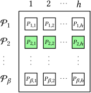
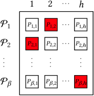
Figure 3: A partitioning system with parameters $(n,\beta,h,k,\eta)$. Each box contains $kn/h$ elements from the ground set $[n]$. Property P1 ensures that selecting an entire row results in low cost (left, in green). Property P2 ensures that selecting one and only one box per each row, for a total of $h$ rows, results in a high cost (right, in red).

To gain some intuition on properties P1 and P2, we provide a graphical representation of a partitioning system in Fig. 3, whereby each box contains $kn/h$ elements from the ground set $[n]$. Property 1 asserts that every time we select an entire row, we are guaranteed to cover every element in $[n]$ precisely $k$ times. Property 2 asserts that every time we select one and only one set from each row, for a total of $h$ rows, many sets cover the same elements so that the resulting cost is high. A concrete example of partitioning system is provided in Fig. 4.

(a)

(b)

(c)

Figure 4: Examples of partitioning systems obtained with the choice of $c(x)=x^{2}$, $k=1$, for increasing values of $\beta=h=2,3,4$ representing the number of rows and columns. Here, each labeled circle represents a resource from the ground set. To verify that (a) is indeed a partitioning system it suffices to observe that, when selecting any entire row, each resource is covered only once (since $k=1$), so that we incur a cost of $4\cdot c(1)=4$ (Property 1), while when selecting one box from each row we incur a cost of $c(1)+c(2)+c(1)=6=\mathbb{E}_{X\sim\text{Bin}(2,1/2)}[X^{2}]$ (Property 2). Analogously for cases (b) and (c). Note how, in these examples, we have been able to construct partitioning systems where the error parameter $\eta$ entering (P2)) is identically zero. Finally, we observe that partitioning systems obtained with $c(x)=x^{2}$, $k=1$ correspond, in the ensuing reduction, to the special case of congestion games with linear resource cost $\ell(x)=x$.

At this stage, we recall that the probability mass function of the binomial distribution $\text{Bin}(h,k/h)$ converges pointwise for fixed $k\geq h$ to the probability mass function of the Poisson distribution $\text{Poi}(k)$ as $h$ grows large (durrett2019probability). Hence, we informally observe that, when $\rho_{\ell}<\infty$,

$$\frac{\sum_{r\in Q}c(|Q|_{r})}{\sum_{r\in\mathcal{P}_{j}}c(|\mathcal{P}_{j}|_{r})}=\frac{\mathbb{E}_{X\sim\text{Bin}(h,k/h)}[c(X)]-\eta}{c(k)}\xrightarrow{h\rightarrow\infty}\frac{\mathbb{E}_{X\sim\text{Poi}(k)}[c(X)]-\eta}{c(k)},$$

see LABEL:lem:convergence in LABEL:app:binomial-poisson for a proof. If we choose $c(x)=x\ell(x)$, let $h\rightarrow\infty$ and consider the worst case over $k$, this ratio precisely matches the inapproximability result we aim to derive (cfr. the previous expression and $\rho_{\ell}$ in (1.1)). We are thus left to piece these elements together in the ensuing section. Before doing so, we remark that partitioning systems do exist for every choice of $\eta>0$ as long as $n$ is taken sufficiently large as stated in the next proposition. Its proof follows the same approach of that in (barman2021tight), and is included in LABEL:subsub:app-proof-partition-exists for completeness. We remark that, when used in the upcoming reduction, we will be able to compute a partitioning systems in time that is independent on the size of the instance we reduce from.

Proposition 2.5

Let $c:\mathbb{N}\rightarrow\mathbb{R}_{>0}$ non-decreasing be given. For every choice of $\beta\geq h\geq k$ integers with $kn/h\in\mathbb{N}$, $\eta\in(0,1)$, and $n\geq\frac{c(h)^{2}}{2\eta^{2}}[\log(10)+\beta\log(h+1)]$ a partitioning system with parameters $(n,\beta,h,k,\eta)$ and cost function $c$ exists. It can be found in time depending solely on $h$, $n$ and $\beta$.

2.2 Reduction

We first provide the reduction and prove the hardness result in the case when $\rho_{\ell}<\infty$. We consider the case $\rho_{\ell}=\infty$ separately at the end of Section 2.3. Starting from the resource cost function $\ell$ and a fixed $\varepsilon>0$, we will first construct a partitioning system with appropriately defined parameters. We then reduce an instance of LabelCover $\mathcal{C}=(L,R,E,h,[\alpha],[\beta],\{\pi_{e}\}_{e\in E})$ to an instance of congestion game $G=(N,\mathcal{R},\{\mathcal{A}_{i}\}_{i=1}^{N},\{\ell_{r}\}_{r\in\mathcal{R}})$ with identical resource cost. The idea is to define $G$ by creating a copy of the partitioning system for every right vertex and use that to define the players’ allocation sets $\mathcal{A}_{i}$.

Construction of the partitioning system. Given $\ell$ and $\varepsilon>0$, we construct a partitioning system setting its parameters as follows:

• Let $k$ be the maximizer of (1.1);

• Let $c$ be the cost function defined from $\ell$ as in $c(x)=x\ell(x)$ for all $x\in\mathbb{N}$ and $c(0)=0$;

• Let $\eta<\min\{\varepsilon c(k)/4,1\}$;

• Let $h\geq k$ integer be such that $|\mathbb{E}_{X\sim\text{Bin}(h,k/h)}[X\ell(X)]-\mathbb{E}_{X\sim\text{Poi}(k)}[X\ell(X)]|\leq\varepsilon c(k)/4$, which exists thanks to the convergence result in LABEL:lem:convergence in LABEL:app:binomial-poisson;

• Let $\delta\leq\varepsilon/(2\rho_{\ell})$ and fix $\beta$ large enough to ensure hardness of GapLabelCover$(\delta,h)$ in Proposition 2.3;

• Let $n$ be so that $kn/h\in\mathbb{N}$ and $n$ is large enough to have existence, from Proposition 2.5, of the partitioning system with parameters $(n,\beta,h,k,\eta)$ and cost function $c$.

Owing to Proposition 2.3, since $\beta,h,k,\eta$ are now fixed, a partitioning system can be computed in time independent of the size of the LabelCover instance we wish to reduce from.

Reduction of LabelCover instance to congestion game instance. Now we take an instance of LabelCover $\mathcal{C}=(L,R,E,h,[\alpha],[\beta],\{\pi_{e}\}_{e\in E})$ where $h$, $\beta$ are defined above and thus Proposition 2.3 (NP-hardness) holds. For each right vertex $u\in R$ we use the local partitioning system with parameters $(n,\beta,h,k,\eta)$. We refer to the resources in the partitioning system corresponding to the right vertex $u\in R$ with $\{1^{u},\dots,n^{u}\}$. Similarly we use $\mathcal{P}^{u}_{j}=\{{P}^{u}_{j,1},\dots,{P}^{u}_{j,h}\}$ for the local partitions. The congestion game $G=(N,\mathcal{R},\{\mathcal{A}_{i}\}_{i=1}^{N},\{\ell_{r}\}_{r\in\mathcal{R}})$ is defined as follows

• each left vertex corresponds to an agent, so that the number of agents is $N=|L|$;

• the ground set of resources is the union of the resources introduced by each local partitioning system on every right vertex, i.e., $\mathcal{R}=\cup_{u\in R}\{1^{u},\dots,n^{u}\}$;

• each resource cost is equal to $\ell$, i.e., $\ell_{r}(x)=\ell(x)$ for all $r\in\mathcal{R}$, $x\in\mathbb{N}$;

• as each left vertex $v\in L$ corresponds to one and only one agent $i\in[N]$, we refer to a left vertex as $i\in[N]$ instead of as $v\in L$ to ease the notation. For agent $i\in[N]$ we construct each pure strategy $a_{i}\in\mathcal{A}_{i}$ as follows. We let the left vertex $i$ select a label $l\in[\alpha]$, and correspondingly take the union over all right vertices $u\in\mathcal{N}(i)$ neighbouring with $i$, of the resources belonging to the block $P^{u}_{j,i}$, where $j=\pi_{(i,u)}(l)$. Repeating over all left labels we obtain the strategy set $\mathcal{A}_{i}$. Formally

  $$\mathcal{A}_{i}=\left\{\cup_{u\in\mathcal{N}(i)}{P}^{u}_{j,i},\quad\text{where}\quad j=\pi_{(i,u)}(l),\quad\forall l\in[\alpha]\right\}.$$

The following figure exemplifies the construction. We conclude remarking that the above procedure implicitly defines a map associating a profile of left labels $(l_{1},\dots,l_{N})$ (one per each left vertex) to an allocation $(a_{1},\dots,a_{N})\in\mathcal{A}$, and that spanning through all possible choices of $(l_{1},\dots,l_{N})$ produces all possible allocations in $\mathcal{A}$. This observation will be useful in proving the hardness result.

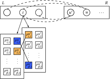
Figure 5: Given a label cover instance $\mathcal{C}=(L,R,E,h,[\alpha],[\beta],\{\pi_{e}\}_{e\in E})$, our reduction associates every left vertex in $L$ to an agent in the game $G$. Here we exemplify how the action set $\mathcal{A}_{i}$ is generated for agent $i\in L$. To ease the presentation, we consider a left alphabet of size $2$ and use blue and orange to identify the left labels. Since $i$ has two right neighbours, $u$ and $u^{\prime}$, we construct two partitioning systems with ground set of resources $\{1^{u},\dots,n^{u}\}$ and $\{1^{u^{\prime}},\dots,n^{u^{\prime}}\}$. Constraints $\pi_{(i,u)}({\tt blue})=1$, $\pi_{(i,u)}({\tt orange})=2$ and $\pi_{(i,u^{\prime})}({\tt blue})=\beta$, $\pi_{(i,u^{\prime})}({\tt orange})=1$ are given, and we represent them graphically with the fact that on the left partitioning system, the label ${\tt blue}$ (resp. ${\tt orange}$) is associated to the block in row $1=\pi_{(i,u)}({\tt blue})$ (resp. row $2=\pi_{(i,u)}({\tt orange})$). Similarly for the right partitioning system using $\pi_{(i,u^{\prime})}$ to determine the row. The set $\mathcal{A}_{i}$ is readily constructed as $\mathcal{A}_{i}=\{P_{1,2}^{u}\cup P^{u^{\prime}}_{\beta,1},P_{2,2}^{u}\cup P^{u^{\prime}}_{1,1}\}$, where the first (resp. second) allocation corresponds to a blue (resp. orange) left label.

2.3 Proof of the result

As anticipated, we first prove the result for the case of $\rho_{\ell}<\infty$. At the end of this section, we turn the attention to $\rho_{\ell}=\infty$. For any given instance of LabelCover $\mathcal{C}=(L,R,E,h,[\alpha],[\beta],\{\pi_{e}\}_{e\in E})$, resource cost $\ell$, and $\varepsilon>0$, we consider an instance of congestion game $G=(N,\mathcal{R},\{\mathcal{A}_{i}\}_{i=1}^{N},\{\ell_{r}\}_{r\in\mathcal{R}})$ constructed as in the previous section. We will now show that

• completeness (Section 2.3.1): If the instance $\mathcal{C}$ is a YES, then $\min_{a\in\mathcal{A}}SC(a)\leq n|R|c(k)$,

• soundness (Section 2.3.2): If the instance $\mathcal{C}$ is a NO, then $\min_{a\in\mathcal{A}}SC(a)>(\rho_{\ell}-\varepsilon)n|R|c(k)$.

An algorithm solving MinSC with an approximation ratio smaller than $\rho_{\ell}-\varepsilon$ will be able to distinguish between YES/NO instances of an NP-hard promise problem. This will conclude the proof.

2.3.1 Completeness

We intend to show that if $\mathcal{C}$ is a YES instance, then $\min_{a\in\mathcal{A}}{\rm{SC}}(a)\leq n|R|c(k)$. This follows readily. In fact, if $\mathcal{C}$ is a YES instance, there exists a labeling that strongly satisfies all right vertices. This implies that there exists an allocation $a^{\ast}\in\mathcal{A}$ whereby, for any given right vertex, all neighbouring left vertices (agents) have selected blocks belonging to an entire row of the corresponding partitioning system. Thanks to property P1 the cost of the allocation $a^{\ast}$ on every local partitioning system is equal to $nc(k)$. Since the total cost is additive over the local partitioning systems, we obtain the result

$$SC(a^{\ast})=n|R|c(k)\implies\min_{a\in\mathcal{A}}SC(a)\leq n|R|c(k).$$

2.3.2 Soundness

We intend to show that if $\mathcal{C}$ is a NO instance, then $\min_{a\in\mathcal{A}}{\rm{SC}}(a)\geq(\rho_{\ell}-\varepsilon)n|R|c(k)$ which is equivalent to showing ${\rm{SC}}(a)\geq(\rho_{\ell}-\varepsilon)n|R|c(k)$ for all $a\in\mathcal{A}$. Towards this goal, we build upon the last observation presented in Section 2.2, i.e., the fact that our construction associates each profile of left labels to an allocation, and that spanning through all possible choices of $(l_{1},\dots,l_{N})$ produces all possible allocations in $\mathcal{A}$. Hence, it suffices to prove the desired property by considering all possible combinations of profiles $(l_{1},\dots,l_{N})$ and the corresponding induced cost, instead of considering all $a\in\mathcal{A}$. Since $\mathcal{C}$ is a NO instance, for any possible choice of $(l_{1},\dots,l_{N})$, no more than $\delta$ fraction of the right vertices are weakly satisfied. Owing to property P2, each partitioning system corresponding to a non weakly satisfied right vertex has a cost larger than $\left(\mathbb{E}_{X\sim\text{Bin}(h,k/h)}[c(X)]-\eta\right)n$. Thus, since at least $(1-\delta)|R|$ right vertices are not weakly satisfied, it is

$${\rm{SC}}(a)\geq\left(\mathbb{E}_{X\sim\text{Bin}(h,k/h)}[c(X)]-\eta\right)(1-\delta)n|R|,\qquad\forall a\in\mathcal{A}.$$

We conclude with some cosmetic manipulation. In particular, we recall that the binomial distribution converges to the Poisson distribution when the number of trials grows large and the success probability of each trial goes to zero (durrett2019probability). In our settings, this corresponds to the fact that the probability mass function of $\text{Bin}(h,k/h)$ converges pointwise for fixed $k$ to that of $\text{Poi}(k)$ as $h\rightarrow\infty$.

Since $\rho_{\ell}<\infty$, we observe that lim_h→∞E_X∼Bin(h,k/h) [c(X)] = E_X∼Poi(k) [c(X)] = ρ_ℓc(k), where equality holds thanks to LABEL:lem:convergence in LABEL:app:binomial-poisson. This implies the existence of a function $\theta(h)$ with $\theta(h)\rightarrow 0$ as $h\rightarrow\infty$ allowing to control the error, and for which $\mathbb{E}_{X\sim\text{Bin}(h,k/h)}[c(X)]\geq\rho_{\ell}c(k)-\theta(h).$ In other words the LHS can be made arbitrarily close to $\rho_{\ell}c(k)$ by selecting $h$ sufficiently large. Hence, SC(a)≥(ρℓc(k)-θ(h) - η)(1-δ)n—R—=[ρℓ- θ(h)c(k)-ηc(k)- (ρℓ- θ(h)c(k)-ηc(k))δ]n —R— c(k)≥[ρℓ- θ(h)c(k)-ηc(k)-ρℓδ]n —R— c(k)¿[ρℓ- ε4- ε4- ε2]n —R— c(k) = (ρℓ-ε)n—R—ck. The last inequality holds by the choice of parameters, ensuring that $\frac{\theta(h)}{c(k)}\leq\frac{\varepsilon}{4}$, $\frac{\eta}{c(k)}<\frac{\varepsilon}{4}$, $\rho_{\ell}\delta\leq\frac{\varepsilon}{2}$.

Case of $\rho_{\ell}=\infty$.

As anticipated, we treat the case of unbounded $\rho_{\ell}$ separately. Towards this goal, we follow the same reduction of Section 2.2, with minor modification on the choice of parameters. We replace $\rho_{\ell}$ with a fixed (and conceptually large) constant $M$. Since $\rho_{\ell}=\infty$, we note that $\mathbb{E}_{X\sim\text{Poi}(k)}[c(X)]/c(k)$ is unbounded at some $k$ (possibly infinity). Since the probability mass functions of $\text{Bin}(h,k/h)$ and $\text{Poi}(k)$ converge, we can choose the pair $h$ and $k$ so that $\mathbb{E}_{X\sim\text{Bin}(h,k/h)}[c(X)]\geq Mc(k)$. Finally, we set $\delta\leq\varepsilon/(2M)$. One then follows the same proof as in the case of bounded $\rho_{\ell}$, whereby (2.3.2) is replaced with ${\rm{SC}}(a)\geq(M-\eta/c(k))(1-\delta)n|R|c(k)\geq(M-\frac{\eta}{c(k)}-M\delta)n|R|c(k)\geq(M-\varepsilon/4-\varepsilon/2)n|R|c(k)>(M-\varepsilon)n|R|c(k)$. Since $M$ can be taken to be arbitrarily large, the problem is NP-hard to approximate within any finite ratio. ∎

2.4 Hardness factor for polynomial resource cost

Corollary 1.2 claims that, when resource costs are obtained by non-negative combinations of monomials of maximum degree $d>0$, MinSC is hard to approximate within any factor smaller than the $(d+1)$’st Bell number. Note that this is a direct consequence of Theorem 1.1 and its ensuing discussion, which applies since for $d\geq 0$, each monomial $x^{d}$ is positive, non-decreasing, semi-convex for $x\in\mathbb{N}$. In this setting, MinSC is NP-hard to approximate within any factor smaller than $\sup_{\ell\in\mathscr{L}}\rho_{\ell}$, where $\mathscr{L}$ contains all polynomials of maximum degree $d$ with non-negative coefficients. Interestingly, LABEL:lem:factor_polynomials in LABEL:app:factor-poly shows that the factor $\rho_{\ell}$ is maximized amongst all polynomials in $\mathscr{L}$ by the monomial $m(x)=x^{d}$. Hence, for polynomial congestion games, it is

$$\sup_{\ell\in\mathscr{L}}\rho_{\ell}=\rho_{m}=\sup_{x\in\mathbb{N}}\frac{\mathbb{E}_{P\sim\text{Poi}(x)}[P^{d+1}]}{x^{d+1}}=\sup_{x\in\mathbb{N}}~{}~{}\sum_{i=0}^{d+1}x^{i-(d+1)}{d+1\brace i}=\sum_{i=0}^{d+1}{d+1\brace i}=\mathcal{B}(d+1).$$

The first equality follows from the fact that $m(x)=x^{d}$ maximizes the ratio $\rho_{\ell}$, while the second from the definition of $\rho_{m}$. The third equality follows from the fact that the $(d+1)$’st moment of the Poisson distribution $\text{Poi}(x)$ equals $\sum_{i=0}^{d+1}x^{i}{d+1\brace i}$, where ${d+1\brace i}$ is a Stirling number of the second kind (mansour2015commutation, p. 63). The fourth equality holds because each function $x^{i-(d+1)}$ is non-increasing, owing to $i\leq(d+1)$, and thus the supremum is attained at $x=1$. The last one is due to the definition of the $(d+1)$’st Bell number, which we denote with $\mathcal{B}(d+1)$, see (mansour2015commutation, Eq. 1.2).

One can repeat a similar reasoning also when $d\geq 0$ is not integer and show that the expression inside the supremum is non-increasing in $x\geq 1$, e.g., by computing its derivatives. If follows that the supremum is attained at $x=1$, and the definition of $\rho_{\ell}$ gives ρ_ℓ=1e∑_i=0^∞id+1i!. The latter expression is sometimes referred to as the fractional Bell number. Note that using Dobiński’s formula (mansour2015commutation, Eq. 1.25), one recovers the Bell number $\mathcal{B}(d+1)$ when $d\in\mathbb{N}_{0}$.

Corollary 1.3 provides a more refined analysis for affine congestion games where $\ell_{r}(x)=\alpha_{r}x+\beta_{r}$, when an upper bound $q$ on $\max_{r}\alpha_{r}/(\alpha_{r}+\beta_{r})$ is given. The proof of Corollary 1.3 follows readily from the application of Theorem 1.1 and its ensuing discussion. Indeed, here one can take the set $\mathscr{L}$ to contain all linear cost functions of the form $\ell(x)=\alpha x+\beta$ where $\alpha/(\alpha+\beta)\leq q$. One can then easily compute $\rho_{\ell}$ explicitly from (1.1)

$$\rho_{\ell}=\sup_{x\in\mathbb{N}}\frac{\mathbb{E}_{P\sim\text{Poi}(x)}[P(\alpha P+\beta)]}{x(\alpha x+\beta)}=\sup_{x\in\mathbb{N}}\frac{\alpha(x^{2}+x)+\beta x}{\alpha x^{2}+\beta x}=1+\frac{\alpha}{\alpha+\beta},$$

and thus obtain the desired hardness factor, i.e., $\sup_{\ell\in\mathscr{L}}\rho_{\ell}=1+q$.

3 Taxes achieve optimal approximation

In this section we show how to compute a taxation mechanism whose price of anarchy matches the hardness factor. Since taxation mechanisms can be utilized to derive polynomial time algorithms with an approximation factor matching the price of anarchy (Section 1.2), in the ensuing LABEL:subsec:comparison-sviri we compare the optimal price of anarchy with the best known polynomial approximation of Makarychev18.

We start by introducing a parameterised family of taxation mechanisms for which we will later provide (efficiently computable) parameters that achieve the desired result. Our taxation mechanisms take as input a congestion game $G$, with resource costs belonging to a common set $\mathscr{L}$. Toward this goal, for each $\ell_{r}:\mathbb{N}\rightarrow\mathbb{R}_{>0}$ given, we extend its definition to $\ell_{r}:\mathbb{N}_{0}\rightarrow\mathbb{R}_{\geq 0}$ by setting $\ell_{r}(0)=0$. This is without loss of generality and merely needed to ease the notation (see Footnote 5 and Footnote 5). For similar reasons, we define $c_{r}:\mathbb{N}_{0}\rightarrow\mathbb{R}_{\geq 0}$ as $c_{r}(x)=x\ell_{r}(x)$ for $x\in\mathbb{N}$ and $c_{r}(0)=0$. Finally, we associate each resource cost $\ell_{r}(x)$ with the function $p_{r}:\mathbb{R}_{\geq 0}\rightarrow\mathbb{R}_{\geq 0}$ defined as p_r(v)= E_P∼Poi(v)[Pℓ_r(P)] = (∑_i=0^∞iℓ_r(i)vii!)e^-v, which we use to introduce the following set of parametrized mechanisms.

Definition 3.1 (Parameterised Taxation Mechanisms)

Given a parameter vector $(v_{r})_{r\in\mathcal{R}}$ with $v_{r}\in\mathbb{R}_{\geq 0}$ and a set of resources $\mathcal{R}$ with costs $\ell_{r}(x)$, define a parameterised taxation function $\tau_{r}:\mathbb{N}_{0}\times\mathbb{R}_{\geq 0}\rightarrow\mathbb{R}_{\geq 0}$, with $\tau_{r}(x,v_{r})=f_{r}(x,v_{r})-\ell_{r}(x)$ where $f_{r}(x,0)=\ell_{r}(x)$, $f_{r}(0,v)=0$, and f_r(x,v)=(x-1)!vx∑_i=0^x-1 pr(v)-iℓr(i)i!v^i,  x∈N_0, v∈R_¿0.

Observe that the previous taxation mechanism effectively substitutes the original resource costs $\ell_{r}(x)$ with the new resource costs $f_{r}(x,v_{r})$ given in (3.1). Indeed, when taxes are factored in, the resource cost perceived by each agent on resource $r$ is $\ell_{r}(x)+\tau_{r}(x,v_{r})=f_{r}(x,v_{r})$. The following lemma provides three important properties of the above class of taxation mechanisms. In particular, Lemma 3.2 ensures that taxes are non-negative, that modified resource costs introduced in (3.1) are non-decreasing and that they satisfy a recursion which will be crucial later on. The proof can be found in LABEL:app:twoproperties.

Lemma 3.2

For all $v\in\mathbb{R}_{\geq 0}$, $x\in\mathbb{N}_{0}$, and $r\in\mathcal{R}$ the taxation mechanism introduced in Definition 3.1 satisfies:

• $\tau_{r}(x,v)\geq 0$,

• $f_{r}(x+1,v)\geq f_{r}(x,v)$,

• $x\ell_{r}(x)-xf_{r}(x,v)+vf_{r}(x+1,v)=p_{r}(v)$.

As we will see in the remainder of the section, the mechanism that optimises the price of anarchy makes use of the parametrized taxation mechanism introduced in Definition 3.1, with parameters obtained by solving the following convex program in the variables $y_{i}$, $v_{r}$ min∑r∈Rpr(vr)subject tovr= ∑i=1N∑k∈[si] : r∈ai,kyi,k for all r∈R, yi∈Δ(si) for all i∈[N], where we let $s_{i}=|\mathcal{A}_{i}|$, $a_{i,k}$, denote the $k$-th action available to player $i$, and $\Delta(s)$ represent the $s$-th dimensional simplex. This program can be easily interpreted as the continuous relaxation of the original MinSC problem, where the resource costs $\ell_{r}$ have been replaced by the modified resource costs $p_{r}$ previously defined.
We are now ready to state our main result of this section, which is an extension of Theorem 1.4. We state the result when $\sup_{\ell\in\mathscr{L}}\rho_{\ell}<\infty$, else the problem is inapproximable as seen in Theorem 1.1.

Theorem 3.3

Consider a congestion game where each resource cost belongs to a common set of functions $\mathscr{L}$ satisfying Assumption 1.1. Let $\sup_{\ell\in\mathscr{L}}\rho_{\ell}<\infty$ and denote with $(\bar{y}_{i})_{i\in[N]},(\bar{v}_{r})_{r\in\mathcal{R}}$ a solution of the convex program (3). Then:

• The taxation mechanism introduced in Definition 3.1 with parameter vector $(\bar{v}_{r})_{r\in\mathcal{R}}$ has a price of anarchy no-higher than $\sup_{\ell\in\mathscr{L}}\rho_{\ell}$;

• Moreover, for any choice of $\varepsilon>0$ one can design in polynomial time, through the approximate solution of (3), a taxation mechanism whose price of anarchy is no-higher than $\sup_{\ell\in\mathscr{L}}\rho_{\ell}+\varepsilon$.

Proof 3.4

Proof. Given a congestion game $G$, we consider the corresponding program (3). Let us verify that (3) is indeed convex. Since the constraints are linear and the objective function is a sum of univariate functions $p_{r}$ it suffices to show that each $p_{r}(v)$ is convex in $v$. This holds true as $p_{r}$ is defined in (3) as the expectation of a convex function over a Poisson distributed random variable. For completeness we provide a proof of this fact in LABEL:lem:pois-is-cvx in LABEL:app:pois-cvx.

Let $(\bar{y}_{i})_{i\in[N]},(\bar{v}_{r})_{r\in\mathcal{R}}$ be an optimal solution of the convex program (3) and consider the taxation mechanism from Definition 3.1 with parameter vector $(\bar{v}_{r})_{r\in\mathcal{R}}$. Denote $\rho=\sup_{\ell\in\mathscr{L}}\rho_{\ell}$.

To complete the proof we will use a smoothness approach, with a crucial modification: Instead of comparing an action profile $a$ (e.g., an equilibrium allocation) with another action profile $a^{\prime}$ (e.g., an optimal allocation), we will compare an action profile $a$ against a mixed profile $y=(y_{1},\dots,y_{N})\in\Delta(s_{1})\times\dots\times\Delta(s_{N})$. Specifically, we will choose the mixed profile $\bar{y}$ solving (3), and show that ∑_i=1^N∑_k=1^s_i ¯y_i,k[¯C_i(a)-